Initial conditions for hydrodynamics from kinetic theory equilibration

Abstract

We use effective kinetic theory to study the pre-equilibrium dynamics in heavy-ion collisions. We describe the evolution of linearized energy perturbations on top of out-of-equilibrium background to the energy-momentum tensor at a time when hydrodynamics becomes applicable. We apply this description to IP-Glasma initial conditions and find an overall smooth transition to hydrodynamics. In a phenomenologically favorable range of $\eta/s$ values, early time dynamics can be accurately described in terms of a few functions of a scaled time variable $\tau T/(\eta/s)$. Our framework can be readily applied to other initial state models to provide the pre-equilibrium dynamics of the energy momentum tensor.

1 Introduction

The expansion of Quark Gluon Plasma fireball in heavy ion collisions is successfully described by relativistic hydrodynamics with small shear viscosity over entropy ratio $\eta/s$ [1, 2, 3]. However, the early time equilibration and isotropization necessary for this hydrodynamic description is outside the scope of hydrodynamics and initial conditions at hydrodynamic initialization time $\tau_{\text{init}}\sim 1\,\text{fm}$ have to be supplied by other models. A desirable pre-equilibrium description would naturally and smoothly transition to hydrodynamics and, therefore, eliminate the dependence on the initialization time $\tau_{\text{init}}$ [4, 5, 6].

In the limit of weak coupling at high collision energies, the early time dynamics can be described by a combination of Color-Glass Condensate (CGC) saturation framework [7, 8, 9] and effective kinetic theory [10, 11]. Classical lattice simulations showed that the so called “bottom-up” is the preferred thermalization scenario in the weak coupling limit [12, 13], and kinetic theory realization of uniform background evolution at moderate values of the coupling constant (which determines the effective $\eta/s$) reaches hydrodynamic behavior in a phenomenologically reasonable time [14]. In this work we describe a practical implementation of kinetic theory pre-equilibration stage for the transverse energy and momentum perturbations [15, 16].

2 Kinetic theory response

Fig. 1: (a) Energy density decomposition to the average and perturbations within a causal circle $|{\bm{x}}-{\bm{x}}_{0}|<c(\tau_{\text{init}}-\tau_{0})$, which determines the system response at $(\tau_{\text{init}},{\bm{x}}_{0})$. (b) Kinetic theory equilibration of boost invariant background energy density in scaled time units $\tau T_{\infty}/(4\pi\eta/s)$, where $T_{\infty}(\tau)\equiv 1/\tau^{1/3}\lim_{\tau\rightarrow\infty}(\tau^{1/3}T(\tau))$. At early times the expansion resembles free streaming, but at late times the evolution agrees with the hydrodynamic gradient expansion given in Eq. (3)

One of the key features of equilibration is the memory loss about the initial state. The late time hydrodynamic evolution of heavy ion collisions is given in terms of the conserved charges (energy and transverse momentum), therefore we use the energy momentum tensor components $T^{\mu\nu}$, i.e. the first moments of the distribution function, to characterize the out-of-equilibrium evolution of particle distribution function $f({\bm{p}},{\bm{x}},\tau)$ in the effective kinetic theory. Causality restricts the system response to its neighborhood, and the time when hydrodynamic description becomes applicable $\tau_{\text{init}}$ is typically short compared to the size of heavy ion collision area. Therefore we use linearized perturbations of the distribution function to calculate the out-of-equilibrium energy momentum tensor perturbations $\delta T^{\rho\sigma}({\bm{x}},\tau)$. Then the total energy momentum tensor at $\tau_{\text{init}}$ can be written as a sum of background $T^{\mu\nu}_{\text{avg}}({\bm{x}},\tau_{\text{init}})$ and the convolution of kinetic theory response function $G_{\rho\sigma}^{\mu\nu}({\bm{x}}-{\bm{x}}^{\prime},\tau_{0},\tau_{\text{init}})$ to initial state perturbations $\delta T^{\rho\sigma}({\bm{x}}^{\prime},\tau_{0})$

$$T^{\mu\nu}({\bm{x}},\tau_{\text{init}})=T^{\mu\nu}_{\text{avg}}({\bm{x}},\tau_{\text{init}})+\int_{|{\bm{x}}-{\bm{x}}^{\prime}|<|\tau_{\text{init}}-\tau_{0}|}\!\!\!\!d^{2}{\bm{x}}^{\prime}G_{\rho\sigma}^{\mu\nu}({\bm{x}}-{\bm{x}}^{\prime},\tau_{0},\tau_{\text{init}})\,\delta T^{\rho\sigma}({\bm{x}}^{\prime},\tau_{0}).$$ (1)

Here the background $T^{\mu\nu}_{\text{avg}}({\bm{x}},\tau_{\text{init}})$ is taken to be uniform and boost invariant within the causal circle (see Fig. 1(a)). The nonlinear background equilibration is described by kinetic theory map $\mathcal{F}$

$$T^{\mu\nu}_{\text{avg}}({\bm{x}},\tau_{\text{init}})=\mathcal{F}\left[T^{\rho\sigma}_{\text{avg}}({\bm{x}},\tau_{0}),\tau_{0},\tau_{\text{ini}}\right],$$ (2)

which is computed by direct simulation. Based on a suitable form of perturbations of the quasi-particle distribution function $f({\bm{x}},{\bm{p}},\tau)$, the coordinate Green functions $G_{\rho\sigma}^{\mu\nu}({\bm{x}}-{\bm{x}}^{\prime},\tau_{0},\tau_{\text{init}})$ are calculated using the linearized evolution of the Boltzmann equation with gluonic elastic scatterings and inelastic particle number changing processes [15, 16].

The expected late time behavior of the boost invariant energy density is given by a hydrodynamic gradient expansion

$${\text{Hydro prediction:}\quad\tau^{4/3}\bar{e}}={(\tau^{4/3}\bar{e})_{\infty}}\bigg{(}\underbrace{\vphantom{C_{2}\bigg{(}\frac{\eta/s}{\tau T}\bigg{)}^{2}}1}_{\text{ideal}}-\underbrace{\vphantom{C_{2}\bigg{(}\frac{\eta/s}{\tau T}\bigg{)}^{2}}\frac{8}{3}\frac{\eta/s}{\tau T}}_{\text{viscous}}+\underbrace{C_{2}\bigg{(}\frac{\eta/s}{\tau T}\bigg{)}^{2}}_{\text{2nd order hydro}}+\ldots\bigg{)}$$ (3)

where $C_{2}$ is a constant depending on the second order transport coefficients. In Fig. 1(b) we compare the background energy evolution in kinetic theory to a second order hydrodynamic asymptotics. Empirically we find that for the relevant range of $\eta/s$ values, equilibration is universal if plotted in units of kinetic theory relaxation time $\tau_{R}={(\eta/s)}/{T}$. Similarly to the background, kinetic theory response functions at the same $\tau/\tau_{R}$ look the same if plotted as a function of radial distance $r/\tau$ in the causal circle (not shown).

3 Results and Conclusions

Fig. 2: Energy density evolution at the center of a fireball after matching to hydrodynamics $\tau_{\text{init}}=0.4,0.8,\text{ and }1.2\,\text{fm}$. The pre-equilibrium evolution $\tau_{0}<\tau<\tau_{\text{init}}$ done in (a) kinetic theory (b) free streaming.

We apply kinetic theory pre-equilibrium evolution to a realistic energy density profile taken from IP-Glasma initial state model at $\tau_{0}=0.2\,\text{fm}$ [17, 18]. The energy perturbations and the background are then propagated to hydrodynamic initialization time $\tau_{\text{init}}$, which is varied. In Fig. 2 we show the energy density evolution at the center of the fireball after matching to hydrodynamics at $\tau_{\text{init}}=0.4,0.8,\text{ and }1.2\,\text{fm}$. We observe that the kinetic theory pre-equilibrium smoothly matches hydrodynamic evolution and the subsequent evolution is largely independent of the switching time $\tau_{\text{init}}$. In contrast, the free streaming evolution does not match hydrodynamics and the late time behavior is sensitive to hydrodynamic initialization time. In Fig. 3 we show the transverse slice of energy density of the same event at different times $\tau$. We see that the transverse profile agrees well between all three hydrodynamic initializations. During the pre-equilibrium evolution the initial energy perturbations also induces a transverse flow, which is an important input in hydrodynamic initialization and can be captured by kinetic theory evolution.

Based on a microscopic description of bottom-up thermalization, we demonstrated the feasibility of event-by-event simulations of the pre-equilibrium dynamics for realistic initial conditions. Naturally our description can be smoothly matched to the subsequent hydrodynamic evolution, thus eliminating the dependence on hydrodynamic initialization time.

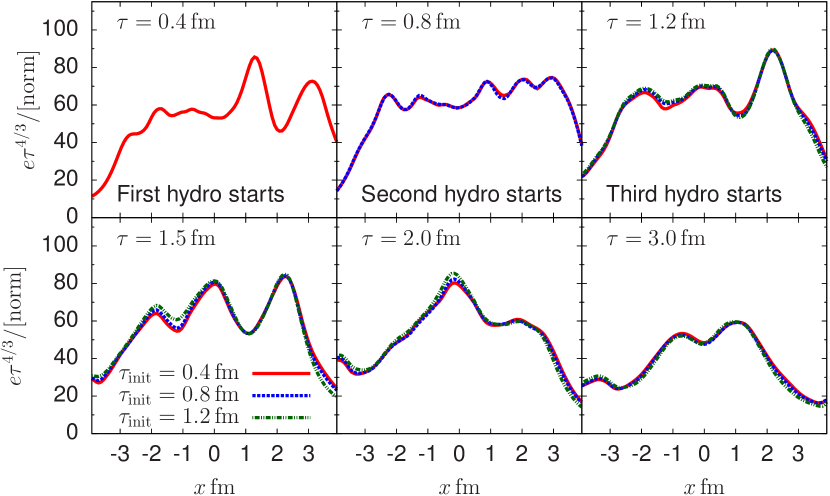
Fig. 3: Transverse slice of energy density after matching to hydrodynamics $\tau_{\text{init}}=0.4,0.8,\text{ and }1.2\,\text{fm}$ with the kinetic theory pre-equilibrium evolution.

Acknowledgments

The authors would like to thank Liam Keegan and Björn Schenke for their contributions at the beginning of this work. Results in this paper were obtained using the high-performance computing system at the Institute for Advanced Computational Science at Stony Brook University. This work was supported in part by the U.S. Department of Energy, Office of Science, Office of Nuclear Physics under Award Numbers DE-FG02-88ER40388 (A.M., J.-F.P., D.T.) and DE-FG02-97ER41014 (S.S.). A.M. would like to thank the organizers of QM 2017 for the student support.

References

- [1] U. Heinz, R. Snellings, Collective flow and viscosity in relativistic heavy-ion collisions, Ann. Rev. Nucl. Part. Sci. 63 (2013) 123–151. arXiv:1301.2826, doi:10.1146/annurev-nucl-102212-170540.
- [2] M. Luzum, H. Petersen, Initial State Fluctuations and Final State Correlations in Relativistic Heavy-Ion Collisions, J. Phys. G41 (2014) 063102. arXiv:1312.5503, doi:10.1088/0954-3899/41/6/063102.
-
[3]
D. A. Teaney,
Viscous
Hydrodynamics and the Quark Gluon Plasma, in: R. C. Hwa, X.-N. Wang (Eds.),
Quark-gluon plasma 4, 2010, pp. 207–266.
arXiv:0905.2433,
doi:10.1142/9789814293297_0004.
URL https://inspirehep.net/record/820552/files/arXiv:0905.2433.pdf - [4] W. van der Schee, P. Romatschke, S. Pratt, Fully Dynamical Simulation of Central Nuclear Collisions, Phys. Rev. Lett. 111 (22) (2013) 222302. arXiv:1307.2539, doi:10.1103/PhysRevLett.111.222302.
- [5] P. Romatschke, Light-Heavy Ion Collisions: A window into pre-equilibrium QCD dynamics?, Eur. Phys. J. C75 (7) (2015) 305. arXiv:1502.04745, doi:10.1140/epjc/s10052-015-3509-3.
- [6] A. Kurkela, Initial state of Heavy-Ion Collisions: Isotropization and thermalization, Nucl. Phys. A956 (2016) 136–143. arXiv:1601.03283, doi:10.1016/j.nuclphysa.2016.01.069.
-
[7]
E. Iancu, A. Leonidov, L. McLerran,
The Color glass
condensate: An Introduction, in: QCD perspectives on hot and dense matter.
Proceedings, NATO Advanced Study Institute, Summer School, Cargese, France,
August 6-18, 2001, 2002, pp. 73–145.
arXiv:hep-ph/0202270.
URL http://alice.cern.ch/format/showfull?sysnb=2297268 - [8] E. Iancu, R. Venugopalan, The Color glass condensate and high-energy scattering in QCD, in: In *Hwa, R.C. (ed.) et al.: Quark gluon plasma* 249-3363, 2003. arXiv:hep-ph/0303204, doi:10.1142/9789812795533_0005.
- [9] F. Gelis, E. Iancu, J. Jalilian-Marian, R. Venugopalan, The Color Glass Condensate, Ann. Rev. Nucl. Part. Sci. 60 (2010) 463–489. arXiv:1002.0333, doi:10.1146/annurev.nucl.010909.083629.
- [10] R. Baier, A. H. Mueller, D. Schiff, D. T. Son, ’Bottom up’ thermalization in heavy ion collisions, Phys. Lett. B502 (2001) 51–58. arXiv:hep-ph/0009237, doi:10.1016/S0370-2693(01)00191-5.
- [11] P. B. Arnold, G. D. Moore, L. G. Yaffe, Effective kinetic theory for high temperature gauge theories, JHEP 01 (2003) 030. arXiv:hep-ph/0209353, doi:10.1088/1126-6708/2003/01/030.
- [12] J. Berges, K. Boguslavski, S. Schlichting, R. Venugopalan, Universal attractor in a highly occupied non-Abelian plasma, Phys. Rev. D89 (11) (2014) 114007. arXiv:1311.3005, doi:10.1103/PhysRevD.89.114007.
- [13] J. Berges, K. Boguslavski, S. Schlichting, R. Venugopalan, Turbulent thermalization process in heavy-ion collisions at ultrarelativistic energies, Phys. Rev. D89 (7) (2014) 074011. arXiv:1303.5650, doi:10.1103/PhysRevD.89.074011.
- [14] A. Kurkela, Y. Zhu, Isotropization and hydrodynamization in weakly coupled heavy-ion collisions, Phys. Rev. Lett. 115 (18) (2015) 182301. arXiv:1506.06647, doi:10.1103/PhysRevLett.115.182301.
- [15] L. Keegan, A. Kurkela, A. Mazeliauskas, D. Teaney, Initial conditions for hydrodynamics from weakly coupled pre-equilibrium evolution, JHEP 08 (2016) 171. arXiv:1605.04287, doi:10.1007/JHEP08(2016)171.
- [16] A. Kurkela, A. Mazeliauskas, J.-F. Paquet, S. Schlichting, D. Teaney, in preparation.
- [17] B. Schenke, P. Tribedy, R. Venugopalan, Fluctuating Glasma initial conditions and flow in heavy ion collisions, Phys. Rev. Lett. 108 (2012) 252301. arXiv:1202.6646, doi:10.1103/PhysRevLett.108.252301.
- [18] B. Schenke, P. Tribedy, R. Venugopalan, Event-by-event gluon multiplicity, energy density, and eccentricities in ultrarelativistic heavy-ion collisions, Phys. Rev. C86 (2012) 034908. arXiv:1206.6805, doi:10.1103/PhysRevC.86.034908.