Fast 2-D Complex Gabor Filter with Kernel Decomposition

Abstract

2-D complex Gabor filtering has found numerous applications in the fields of computer vision and image processing. Especially, in some applications, it is often needed to compute 2-D complex Gabor filter bank consisting of the 2-D complex Gabor filtering outputs at multiple orientations and frequencies. Although several approaches for fast 2-D complex Gabor filtering have been proposed, they primarily focus on reducing the runtime of performing the 2-D complex Gabor filtering once at specific orientation and frequency. To obtain the 2-D complex Gabor filter bank output, existing methods are repeatedly applied with respect to multiple orientations and frequencies. In this paper, we propose a novel approach that efficiently computes the 2-D complex Gabor filter bank by reducing the computational redundancy that arises when performing the Gabor filtering at multiple orientations and frequencies. The proposed method first decomposes the Gabor basis kernels to allow a fast convolution with the Gaussian kernel in a separable manner. This enables reducing the runtime of the 2-D complex Gabor filter bank by reusing intermediate results of the 2-D complex Gabor filtering computed at a specific orientation. Furthermore, we extend this idea into 2-D localized sliding discrete Fourier transform (SDFT) using the Gaussian kernel in the DFT computation, which lends a spatial localization ability as in the 2-D complex Gabor filter. Experimental results demonstrate that our method runs faster than state-of-the-arts methods for fast 2-D complex Gabor filtering, while maintaining similar filtering quality.

I Introduction

2-D complex Gabor filter has been widely used in numerous applications of computer vision and image processing thanks to its elegant properties of extracting locally-varying structures from an image. In general, it is composed of the Gaussian kernel and complex sinusoidal modulation term, which can be seen as a special case of short time discrete Fourier transform (STFT). The Gabor basis functions defined for each pixel offer good spatial-frequency localization [1].

It was first discovered in [2] that the 2D receptive field profiles of simple cells in the mammalian visual cortex can be modeled by a family of Gabor filters. It was also known in [3, 4] that image analysis approaches based on the Gabor filter conceptually imitate the human visual system (HVS). The 2-D complex Gabor filter is invariant to rotation, scale, translation and illumination [5], and it is particularly useful for extracting features at a set of different orientations and frequencies from the image. Thanks to such properties, it has found a great variety of applications in the field of computer vision and image processing, including texture analysis [6, 7, 8, 9], face recognition [10, 11, 12, 13, 14], face expression recognition [15, 16] and fingerprint recognition [17].

Performing the 2-D complex Gabor filtering for all pixels over an entire image, however, often provokes a heavy computational cost. With the 2-D complex Gabor kernel defined at specific orientation and frequency, the filtering is performed by moving a reference pixel to be filtered one pixel at a time. The complex kernel hinders the fast computation of the 2-D complex Gabor filtering in the context similar to edge-aware filters [18, 19, 20] that are widely used in numerous computer vision applications.

To expedite the 2-D complex Gabor filtering, several efforts have been made, for instance, by making use of the fast Fourier transform (FFT), infinite impulse response (IIR) filters, or finite impulse response (FIR) filters [21, 22, 23, 24]. It is shown in [21] that the Gabor filtering and synthesis for a 1-D signal consisting of $N$ samples can be performed with the same complexity as the FFT, $O(NlogN)$. In [22], separable FIR filters are applied to implement fast 2-D complex Gabor filtering by exploiting particular relationships between the parameters of the 2-D complex Gabor filter in a multiresolution pyramid. The fast pyramid implementation is, however, feasible only for the particular setting of Gabor parameters, e.g., scale of $2^{i}$ with an integer $i$. Young et al. [23] proposes to formulate the 2-D complex Gabor filter as IIR filters that efficiently work in a recursive manner. They decompose the Gabor filter with multiple IIR filters through z-transform, and then performs the recursive filtering in a manner similar to recursive Gaussian filtering [25]. To the best of our knowledge, the fastest algorithm for the 2-D complex Gabor filtering is the work of Bernardino and Santos-Victor [24] that decomposes the 2-D complex Gabor filtering into more efficient Gaussian filtering and sinusoidal modulations. It was reported in [24] that this method reduces up to $39\%$ the number of arithmetic operations compared to the recursive Gabor filtering [23].

These fast methods mentioned above primarily focus on reducing the runtime of performing the 2-D complex Gabor filtering once at specific orientation and frequency. However, in some computer vision applications, it is often needed to compute the 2-D complex Gabor filter bank consisting of the 2-D complex Gabor filtering outputs at multiple orientations and frequencies. For instance, face recognition approaches relying on the 2-D Gabor features usually require performing the 2-D complex Gabor filtering at 8 orientations and 5 frequencies (totally, 40 Gabor feature maps) to deal with geometric variances [10, 11, 13, 26, 14]. Fig. 1 shows the example of the filter kernels used in the 2-D complex Gabor filter bank. To compute the complex Gabor filter bank, existing approaches simply repeat the Gabor computation step for a given set of frequencies and orientations without considering the computational redundancy that exists in such repeated calculations.

In this paper, we propose a novel approach that efficiently compute 2-D complex Gabor filter bank by reducing the computational redundancy that arises when performing the 2-D complex Gabor filtering at multiple orientations and frequencies. We first decompose the Gabor basis kernels by making use of the trigonometric identities. This allows us to perform a fast convolution with the Gaussian kernel in a separable manner for $x$ and $y$ dimensions. More importantly, our decomposition strategy enables the substantial reduction of the computational complexity when computing the 2-D complex Gabor filter bank at a set of orientations and frequencies. In our formulation, intermediate results of the 2-D complex Gabor filtering computed at a specific orientation can be reused when performing the 2-D complex Gabor filtering at a symmetric orientation. This is particularly useful in some applications where the 2-D complex Gabor filtering outputs at various orientations and frequencies are needed to cope with geometric variations [10, 11, 5, 13, 14, 26, 9]. We will show that our method reduces the computational complexity when compared to state-of-the-art methods [23, 24], while maintaining the similar filtering quality.

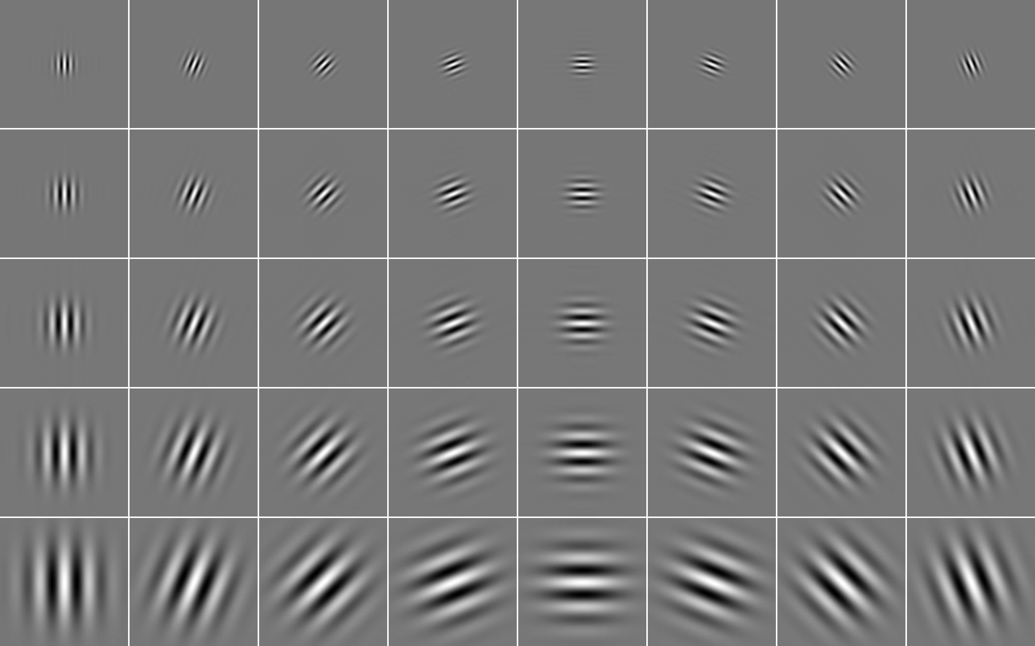
Figure 1: Example of the 2-D complex Gabor filter bank with 40 coefficients (5 frequencies and 8 orientations). The coefficients are computed by $\omega=2^{-(i+2)/2}$ ($i=0,...,4$), $\theta=k\pi/8$ ($k=0,...,7$) and $\sigma=2\pi/\omega$[10].

Additionally, we present a method that efficiently computes 2-D localized sliding discrete Fourier transform (SDFT) using the Gaussian kernel at the transform window by extending the proposed kernel decomposition technique. In literature, the 2-D SDFT usually performs the transform at an image patch within the transform window by shifting the window one pixel at a time in either horizontal or vertical directions. Numerous methods have been proposed for the fast computation of the 2-D SDFT [27, 28, 29]. For instance, the relation between two successive 2-D DFT outputs is first derived using the circular shift property [29]. Using this relation, the 2-D DFT output at the current window is efficiently updated by linearly combining the 2-D DFT output at the previous window and one 1-D DFT result only. Note that all these methods use a box kernel within the sliding transform window and the circular shift property holds only when the box kernel is employed. Therefore, applying the existing 2-D SDFT methods [27, 28, 29] are infeasible in the case of calculating the localized DFT outputs with the Gaussian kernel.

It is generally known that the good spatial localization of the Gabor filter mainly benefits from the use of the Gaussian kernel which determines an weight based on a spatial distance. We will present that the fast computation method of the 2-D localized SDFT using the Gaussian kernel, which lends the spatial localization ability as in the Gabor filter, is also feasible using our decomposition strategy. It should be noted that existing fast 2-D complex Gabor filters [23, 24] can be readily used to compute the 2-D localized SDFT, but a direct application of theses methods disregards the computational redundancy that exists on the repeated calculation of 2-D DFT outputs at multiple frequencies as in the 2-D complex Gabor filter bank. We will show that our method outperforms existing approaches [23, 24] in terms of computational complexity.

To sum up, our contributions can be summarized as follows.

• A new method is presented for efficiently computing the 2-D complex Gabor filter bank at a set of orientations and frequencies. We show that our method runs faster than existing approaches.

• The proposed method is extended into the 2-D localized SDFT, demonstrating a substantial runtime gain over existing approaches.

• Extensive comparison with state-of-the-arts approaches is given in both analytic and experimental manners.

The rest of this paper is organized as follows. In Section II, we present the proposed method for fast computation of the 2-D complex Gabor filter bank. In Section III, we present how the proposed approach is extended to accelerate the 2-D localized SDFT. Section IV presents experimental results including runtime and filtering quality comparison with state-of-the-arts methods. Section V concludes this paper with some remarks.

II Fast 2-D Complex Gabor Filter

This section presents a new method that efficiently computes the 2-D complex Gabor filter bank consisting of the 2-D complex Gabor filtering outputs at multiple orientations and frequencies. We first explain the Gabor kernel decomposition method to reduce the complexity of 2-D complex Gabor filtering, and then show how the decomposition method can be used for fast computation of 2-D complex Gabor filter bank.

For specific orientation $\theta$ and frequency $\omega$, the 2-D complex Gabor filtering output $F_{\omega,\theta,\sigma}$ of a 2-D image $f$ of $H\times W$ can be written as

$$\begin{split}F_{\omega,\theta,\sigma}(x,y)=\sum\limits_{l,k}f(k,l)C_{\omega,\theta}(x-k,y-l){G_{\sigma}}(x-k,y-l)\end{split}$$ (1)

where $G_{\sigma}(x,y)$ is 2-D Gaussian function with zero mean and the standard deviation of $\sigma$. Here, an isotropic Gaussian kernel that has the same standard deviation for both $x$ and $y$ dimensions is used as in existing work [23, 24], i.e., $G_{\sigma}(x,y)=S_{\sigma}(x)S_{\sigma}(y)$. The complex exponential function $C_{\omega,\theta}(x,y)$ for orientation $\theta$ and frequency $\omega=2\pi/\lambda$, where $\lambda$ represents wavelength, is defined as

$$C_{\omega,\theta}(x,y)=e^{i\omega\left(x\cos\theta+y\sin\theta\right)}.$$ (2)

This is decomposed as $C_{\omega,\theta}(x,y)=H_{\omega,\theta}(x)V_{\omega,\theta}(y)$ with $H_{\omega,\theta}(x)=e^{i\omega x\cos\theta}$, $V_{\omega,\theta}(y)=e^{i\omega y\sin\theta}$.

II-A Kernel Decomposition

Since $G_{\sigma}(x,y)$ and $C_{\omega,\theta}(x,y)$ are separable for $x$ and $y$ dimensions, (1) can be rewritten as

$$J_{\omega,\theta,\sigma}(x,y)=\sum\limits_{k}f(k,y)H_{\omega,\theta}(x-k){S_{\sigma}}(x-k),\\$$ (3)

$$F_{\omega,\theta,\sigma}(x,y)=\sum\limits_{l}J_{\omega,\theta,\sigma}(x,l)V_{\omega,\theta}(y-l){S_{\sigma}}(y-l),$$ (4)

$J_{\omega,\theta,\sigma}$ is first computed by performing 1-D horizontal Gabor filtering and this is then used in 1-D vertical filtering for obtaining the final Gabor output $F_{\omega,\theta,\sigma}$.

II-A1 Horizontal 1-D Gabor Filtering

We first present the efficient computation of $J_{\sigma,\omega,\theta}$ in (3) based on the basis decomposition using the trigonometric identities. We explain the real part of $J_{\sigma,\omega,\theta}$ only, as its imaginary counterpart can be decomposed in a similar manner. For the sake of simplicity, we define $\omega^{c}_{\theta}=\omega\cos\theta$ and $\omega^{s}_{\theta}=\omega\sin\theta$. We also omit $y$ in the computation of $J_{\sigma,\omega,\theta}$ and $f$ as the 1-D operation is repeated for $y=1,...,H$. Using the trigonometric identity $\cos(a-b)=\cos a\cos b+\sin a\sin b$, we can simply decompose (3) into two terms as

$$\mathcal{R}\{J_{\omega,\theta,\sigma}(x)\} =\cos(\omega^{c}_{\theta}x)\sum\limits_{k}{f_{c}(k){S_{\sigma}}(x-k)}$$

$$+\sin(\omega^{c}_{\theta}x)\sum\limits_{k}{f_{s}(k){S_{\sigma}}(x-k)},$$ (5)

where $f_{c}(k)=f(k)\cos(\omega^{c}_{\theta}k)$ and $f_{s}(k)=f(k)\sin(\omega^{c}_{\theta}k)$. $\mathcal{R}(F)$ represents the real part of $F$. Then, (II-A1) can be simply computed by applying the Gaussian smoothing to two modulated signals $f_{c}$ and $f_{s}$, respectively. The imagery counterpart $\mathcal{I}\{F\}$ can be expressed similarly as

$$\mathcal{I}\{J_{\omega,\theta,\sigma}(x)\} =-\cos(\omega^{c}_{\theta}x)\sum\limits_{k}{f_{s}(k){S_{\sigma}}(x-k)}$$

$$+\sin(\omega^{c}_{\theta}x)\sum\limits_{k}{f_{c}(k){S_{\sigma}}(x-k)}.$$ (6)

Interestingly, both real and imagery parts of $F$ contains the Gaussian convolution with $f_{c}$ and $f_{s}$, thus requiring only two 1-D Gaussian smoothing in computing (II-A1) and (II-A1). Many methods have been proposed to perform fast Gaussian filtering [30, 25], where the computational complexity per pixel is independent of the smoothing parameter $\sigma$. Here, we adopted the recursive Gaussian filtering proposed by Young and Vliet [25].

II-A2 Vertical 1-D Gabor Filtering

After $J(x,y)$ is computed using (II-A1) and (II-A1) for all $y=1,..,H$, we perform the 1-D Gabor filtering on the vertical direction using (4). Note that the input signal $J$ in (4) is complex, different from the real input signal $f$ in (3). Using the trigonometric identity, we decompose the real and imagery parts of $F$ in (4) as follows:

$${\cal R}\{{F_{\omega,\theta,\sigma}(x,y)}\} =\cos(\omega_{\theta}^{s}y)\left({f^{\prime}_{cr}(x,y)+f^{\prime}_{si}(x,y)}\right)$$

$$+\sin(\omega_{\theta}^{s}y)\left({f^{\prime}_{sr}(x,y)-f^{\prime}_{ci}(x,y)}\right),$$ (7)

$${\cal I}\{{F_{\omega,\theta,\sigma}(x,y)}\} =\sin(\omega_{\theta}^{s}y)\left({f^{\prime}_{cr}(x,y)+f^{\prime}_{si}(x,y)}\right)$$

$$-\cos(\omega_{\theta}^{s}y)\left({f^{\prime}_{sr}(x,y)-f^{\prime}_{ci}(x,y)}\right).$$ (8)

Here, $f^{\prime}_{cr}$, $f^{\prime}_{sr}$, $f^{\prime}_{ci}$, and $f^{\prime}_{si}$ are filtering results convolved with 1-D Gaussian kernel $S_{\sigma}$ as follows:

$$\begin{array}[]{l}f^{\prime}_{cr}(x,y)+f^{\prime}_{si}(x,y)=\sum\limits_{l}{(f_{cr}(x,l)+f_{si}(x,l)){S_{\sigma}}(y-l)},\\ f^{\prime}_{sr}(x,y)-f^{\prime}_{ci}(x,y)=\sum\limits_{l}{(f_{sr}(x,l)-f_{ci}(x,l)){S_{\sigma}}(y-l)},\end{array}$$ (9)

where the modulated signals $f_{cr}$, $f_{sr}$, $f_{ci}$, and $f_{si}$ are defined as

$$\begin{array}[]{l}f_{cr}(x,y)=\mathcal{R}\{J_{\omega,\theta,\sigma}(x,y)\}\cos(\omega^{s}_{\theta}y),\\ f_{sr}(x,y)=\mathcal{R}\{J_{\omega,\theta,\sigma}(x,y)\}\sin(\omega^{s}_{\theta}y),\\ f_{ci}(x,y)=\mathcal{I}\{J_{\omega,\theta,\sigma}(x,y)\}\cos(\omega^{s}_{\theta}y),\\ f_{si}(x,y)=\mathcal{I}\{J_{\omega,\theta,\sigma}(x,y)\}\sin(\omega^{s}_{\theta}y).\end{array}$$ (10)

Like the horizontal filtering, two 1-D Gaussian convolutions are required in (II-A2) and (II-A2), i.e., $f^{\prime}_{cr}(x,l)+f^{\prime}_{si}(x,l)$ and $f^{\prime}_{sr}(x,l)-f^{\prime}_{ci}(x,l)$.

In short, decomposing the complex exponential basis function $C_{\omega,\theta}$ enables us to apply fast Gaussian filtering [30, 25]. Though the fast Gaussian filter was used for implementing fast recursive Gabor filtering in [23], our method relying on the trigonometric identity and separable implementation for $x$ and $y$ dimensions results in a lighter computational cost than the state-of-the-arts method [23]. More importantly, we will show this decomposition further reduces the computational complexity when computing the 2-D complex Gabor filter bank.

II-B Fast Computation of 2-D Complex Gabor Filter Bank

Several computer vision applications often require computing the 2-D complex Gabor filter bank consisting of a set of 2-D complex Gabor filtering outputs at multiple frequencies and orientations. For instance, in order to deal with geometric variances, some face recognition approaches use the 2-D complex Gabor filtering outputs at 8 orientations and 5 frequencies (see Fig. 1) as feature descriptors [10, 11, 13, 26, 14]. To compute the 2-D complex Gabor filter bank, existing approaches repeatedly perform the 2-D complex Gabor filtering for a given set of frequencies and orientations, disregarding the computational redundancy that exists in such repeated calculations.

In this section, we present a new method that efficiently computes the 2-D complex Gabor filter bank. Without the loss of generality, it is assumed that the standard deviation $\sigma$ of the Gaussian kernel is fixed. For a specific frequency $\omega$, we aim at computing the 2-D complex Gabor filter bank at $N$ orientations $\{\frac{\pi k}{N}|k=0,...,N-1\}$. Here, $N$ is typically used as an even number. For the simplicity of notation, we omit $\omega$ and $\sigma$ in all equations. Let us assume that $F_{\theta}$ in (4) is computed using the proposed kernel decomposition technique and its intermediate results are stored. We then compute $F_{\pi-\theta}$ by recycling these intermediate results. The separable form of $F_{\pi-\theta}$ can be written as

$$J_{\pi-\theta}(x,y)=\sum\limits_{k}f(k,y)H_{\omega,\pi-\theta}(x-k){S_{\sigma}}(x-k).$$ (11)

$$F_{\pi-\theta}(x,y)=\sum\limits_{l}J_{\pi-\theta}(x,l)V_{\omega,\pi-\theta}(y-l){S_{\sigma}}(y-l)$$ (12)

Using $H_{\omega,\pi-\theta}(x)=H^{*}_{\omega,\theta}(x)$, where $*$ denotes complex conjugation, (11) can be rewritten as follows:

$$J_{\pi-\theta}(x,y)=J^{*}_{\theta}(x,y).$$ (13)

The horizontal 1-D Gabor filtering result $J_{\pi-\theta}$ is complex conjugate to $J_{\theta}$. Using $V_{\omega,\pi-\theta}(x)=V_{\omega,\theta}(x)$, the vertical 1-D Gabor filtering in (12) is then expressed as

$$F_{\pi-\theta}(x,y) =\sum\limits_{l}J^{*}_{\theta}(x,l)V_{\omega,\theta}(y-l){S_{\sigma}}(y-l).$$ (14)

$F_{\pi-\theta}$ is obtained by applying the vertical 1-D Gabor filtering to the complex conjugate signal $J^{*}_{\theta}$. Using (II-A2) and (II-A2), the following equations are derived:

$${\cal R}\{{F_{\pi-\theta}(x,y)}\} =\cos(\omega_{\theta}^{s}y)\left({f^{\prime}_{cr}(x,y)-f^{\prime}_{si}(x,y)}\right)$$

$$+\sin(\omega_{\theta}^{s}y)\left({f^{\prime}_{sr}(x,y)+f^{\prime}_{ci}(x,y)}\right),$$ (15)

$${\cal I}\{{F_{\pi-\theta}(x,y)}\} =\sin(\omega_{\theta}^{s}y)\left({f^{\prime}_{cr}(x,y)-f^{\prime}_{si}(x,y)}\right)$$

$$-\cos(\omega_{\theta}^{s}y)\left({f^{\prime}_{sr}(x,y)+f^{\prime}_{ci}(x,y)}\right)$$ (16)

The vertical filtering also requires two Gaussian convolutions. Algorithm 1 summarizes the proposed method for computing the 2-D complex Gabor filter bank. When a set of frequencies $\Omega$ and orientations $\Theta$ are given, we compute the 2-D complex Gabor filtering results at $\theta_{k}$ ($k=0,...,N-1$) with the frequency $\omega_{i}$ being fixed. Different from existing approaches [23, 24] repeatedly applying the 2-D complex Gabor filter at all orientations, we consider the computational redundancy that exists on such repeated calculations to reduce the runtime. We will demonstrate our method runs faster than existing fast Gabor filters [23, 24] through both experimental and analytic comparisons.

Algorithm 1 Pseudo code of 2-D complex Gabor filter bank

1:Input: input image $f$ ($H\times W$),

2:    a set of $O$ scales $\Sigma=\{\sigma_{i}|i=0,...,O-1\}$,

3:    a set of $O$ frequencies $\Omega=\{\omega_{i}|i=0,...,O-1\}$,

4:    a set of $N$ orientations $\Theta=\{\theta_{k}|k=0,...,N-1\}$

5:Output: 2-D complex Gabor filter outputs for $\Omega$ and $\Theta$

6:for $i=0,...,O-1$ do $\triangleright$ For all frequencies

7:     $\sigma_{i}=2\pi/\omega_{i},N_{h}=\lfloor N/2\rfloor$

8:     for $k=0,...,N_{h}$ do $\triangleright$ For half of all orientations

9:         $\theta_{k}=\pi k/N$

10:         for $y=1,...,H$ do

11:              Perform 1-D Gaussian filtering of $f_{c},f_{s}$

12:              Compute $J_{\omega_{i},\theta_{k},\sigma_{i}}(x,y)$ for all $x$ in (II-A1) and (II-A1)

13:         end for

14:         for $x=1,...,W$ do

15:              Perform 1-D Gaussian filtering of $f_{cr}+f_{si}$,     $f_{sr}-f_{ci}$ in (II-A2) and (II-A2)

16:              Compute $F_{\omega_{i},\theta_{k},\sigma_{i}}(x,y)$ for all $y$

17:         end for

18:     end for

19:     for $k=N_{h}+1,...,N-1$ do $\triangleright$ For remaining ori.

20:         $\theta_{k}=\pi k/N$

21:         $J_{\omega_{i},\theta_{k},\sigma_{i}}(x,y)=J^{*}_{\omega_{i},\pi-\theta_{k},\sigma_{i}}(x,y)$ for all $x$ and $y$.

22:         for $x=1,...,W$ do

23:              Perform 1-D Gaussian filtering of $f_{cr}-f_{si}$,     $f_{sr}+f_{ci}$ in (II-A2) and (II-A2)

24:              Compute $F_{\omega_{i},\theta_{k},\sigma_{i}}(x,y)$ for all $y$

25:         end for

26:     end for

27:end for

III Localized Sliding DFT

It is known that the Gabor filter offers the good spatial localization thanks to the Gaussian kernel that determines an weight based on a spatial distance. Inspired by this, we present a new method that efficiently compute the 2-D localized SDFT using the proposed kernel decomposition technique. Different from the existing 2-D SDFT approaches [27, 28, 29] using the box kernel, we use the Gaussian kernel when computing the DFT at the sliding window as in the Gabor filter. It should be noted that applying the existing 2-D SDFT approaches [27, 28, 29] are infeasible in the case of calculating the DFT outputs with the Gaussian kernel.

III-A Kernel decomposition in 2-D localized SDFT

When the sliding window of $M\times M$ is used, we set the standard deviation $\sigma$ of the Gaussian kernel by considering a cut-off range, e.g., $\lfloor M/2\rfloor=3\sigma$. We denote $F_{u,v}(x,y)$ by the $(u,v)^{th}$ bin of the $M\times M$ DFT at $(x,y)$ of 2-D image $f$. The 2-D localized SDFT with the Gaussian kernel can be written as

$$F_{u,v} (x,y)=$$

$${\sum\limits_{n,m}{f(m,n)C_{u,v}(\widehat{x}-m,\widehat{y}-n)G_{\sigma}(x-m,y-n)}}$$ (17)

where $\widehat{x}=x-\frac{M}{2}$ and $\widehat{y}=y-\frac{M}{2}$. For $u,v=0,...,M-1$, the complex exponential function $C_{u,v}(m,n)$ at the $(u,v)^{th}$ frequency is defined as

$$C_{u,v}(x,y)=e^{i(\omega_{0}ux+\omega_{0}vy)},$$ (18)

where $\omega_{0}=\frac{2\pi}{M}$. Note that in (III-A) and (18), slightly different notations than the conventional SDFT methods [27, 28, 29] are used to keep them consistent with the Gabor filter of (1). When $G_{\sigma}(x,y)=1$, (III-A) becomes identical to that of the conventional SDFT methods [27, 28, 29]. The Gaussian window of $M\times M$ is used here, but the 2-D localized SDFT using $M_{y}\times M_{x}$ window ($M_{y}\neq M_{x}$) is also easily derived.

Using the separable property of $G_{\sigma}(x,y)=S_{\sigma}(x)S_{\sigma}(y)$ and $C_{u,v}(x,y)=H_{u}(x)V_{v}(y)$, (III-A) can be written as

$$J_{u}(x,y)=\sum\limits_{m}{f(m,y)H_{u}(\widehat{x}-m)S_{\sigma}(x-m)},$$ (19)

$$F_{u,v}(x,y)=\sum\limits_{n}{J_{u}(x,n)V_{v}(\widehat{y}-n)S_{\sigma}(y-n)}.$$ (20)

Using the kernel decomposition, the 1-D horizontal localized SDFT is performed as follows:

$$\mathcal{R}\{J_{u}(x)\} =\cos(\omega_{0}u\widehat{x})\sum\limits_{m}{f_{c}(m){S_{\sigma}}(x-m)}$$

$$+\sin(\omega_{0}u\widehat{x})\sum\limits_{m}{f_{s}(m){S_{\sigma}}(x-m)},$$ (21)

$$\mathcal{I}\{J_{u}(x)\}= -\cos(\omega_{0}u\widehat{x})\sum\limits_{m}{f_{s}(m){S_{\sigma}}(x-m)}$$

$$+\sin(\omega_{0}u\widehat{x})\sum\limits_{m}{f_{c}(m){S_{\sigma}}(x-m)},$$ (22)

where $f_{c}(m)=f(m)cos(\omega_{0}um)$, $f_{s}(m)=f(m)sin(\omega_{0}um)$.

The vertical 1-D localized SDFT is performed similar to the Gabor filter:

$${\cal R}\{{F_{u,v}(x,y)}\} =\cos(\omega_{0}v\widehat{y})\left({f^{\prime}_{cr}(x,y)+f^{\prime}_{si}(x,y)}\right)$$

$$+\sin(\omega_{0}v\widehat{y})\left({f^{\prime}_{sr}(x,y)-f^{\prime}_{ci}(x,y)}\right),$$ (23)

$${\cal I}\{{F_{u,v}(x,y)}\} =\sin(\omega_{0}v\widehat{y})\left({f^{\prime}_{cr}(x,y)+f^{\prime}_{si}(x,y)}\right)$$

$$-\cos(\omega_{0}v\widehat{y})\left({f^{\prime}_{sr}(x,y)-f^{\prime}_{ci}(x,y)}\right),$$ (24)

where $f^{\prime}_{cr}+f^{\prime}_{si}$ and $f^{\prime}_{sr}-f^{\prime}_{ci}$ are defined in a manner similar to (9).

III-B Exploring Computational Redundancy on $(u,v)$

The 2-D localized SDFT requires computing a set of DFT outputs for $u,v=0,...,M-1$, similar to the 2-D complex Gabor filter bank. Considering the conjugate symmetry property of the DFT ($F_{M-u,M-v}=F^{*}_{u,v}$), we compute the DFT outputs $F_{u,v}$ only for $u=0,...,M-1$ and $v=0,...,\lfloor M/2\rfloor$, and then simply compute remaining DFT outputs (for $u=0,...,M-1$ and $v=\lfloor M/2\rfloor+1,...,M-1$) by using the complex conjugation. Thus, we focus on the computation of the 2-D SDFT for $u=0,...,M-1$ and $v=0,...,\lfloor M/2\rfloor$.

Let us consider how to compute $F_{M-u,v}$ using intermediate results of $F_{u,v}$. Similar to the Gabor filter bank, the 1-D DFT $J_{M-u}$ is complex conjugate to $J_{u}$ as follows:

$$J_{M-u}(x,y) =\sum\limits_{m}{f(m,y)H_{M-u}(\widehat{x}-m)S_{\sigma}(x-m)},$$

$$=\sum\limits_{m}{f(m,y)H^{*}_{u}(\widehat{x}-m)S_{\sigma}(x-m)},$$

$$=J^{*}_{u}(x,y)$$ (25)

The 1-D vertical SDFT result $F_{M-u,v}$ is then obtained as

$$F_{M-u,v}(x,y)=\sum\limits_{n}{J^{*}_{u}(x,n)V_{v}(\widehat{y}-n)S_{\sigma}(y-n)}.$$ (26)

As in the Gabor filter bank, (26) can be computed by performing the 1-D vertical Gaussian filtering twice.

Fig. 2 visualizes the log polar grid of the 2-D complex Gabor filter and the regular grid of the 2-D SDFT. There exists an additional computational redundancy when performing the 2-D SDFT on the regular grid. Specifically, for a specific $u$, the 1-D horizontal filtering results $J_{u}(x,y)$ remain unchanged for $v=0,...,\lfloor M/2\rfloor$. These intermediate results can be used as inputs for the 1-D vertical localized SDFT for $v=0,...,\lfloor M/2\rfloor$.

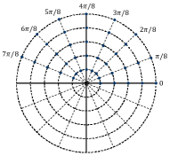
(a) Log polar grid

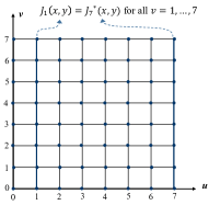
(b) Rectangular grid

Figure 2: Log polar grid of the 2-D complex Gabor filter and the rectangular grid of the 2-D SDFT. (a) 5 frequencies and 8 orientations, (b) $8\times 8$ window ($M=8$). In the log polar grid, two 1-D horizontal Gabor outputs are complex conjugate, i.e., $J_{\omega,\theta,\sigma}=J^{*}_{\omega,\pi-\theta,\sigma}$, when $\omega$ is fixed. In the 2-D SDFT, $J_{u}=J_{M-u}$ holds for $v=0,...,M-1$. These intermediate results can be reused in the computation of Gabor filter bank and the 2-D localized SDFT.

Algorithm 2 Pseudo code of 2-D Localized SDFT

1:Input: input image $f$ ($H\times W$), scale $\sigma$, kernel size $M_{y}\times M_{x}$ ($M_{y}\geq M_{x}$)

2:Output: SDFT outputs at $u=0,...,M_{x}-1$ and $v=0,...,M_{y}-1$

3:$M_{xh}=\lfloor M_{x}/2\rfloor$, $M_{yh}=\lfloor M_{y}/2\rfloor$

4:for $u=0,...,M_{xh}$ do

5:     for $y=1,...,H$ do $\triangleright$ 1-D horizontal SDFT

6:         Perform 1-D Gaussian filtering of $f_{c},f_{s}$  in (III-A) and (III-A).

7:         Compute $J_{u}(x,y)$ for all $x$.

8:     end for

9:end for

10:for $u=M_{xh}+1,...,M_{x}-1$ do

11:     $J_{M_{x}-u}(x,y)=J^{*}_{u}(x,y)$ for all $x$ and $y$.

12:end for

13:for $u=0,...,M_{x}-1$, $v=0,...,M_{yh}$ do

14:     for $x=1,...,W$ do $\triangleright$ 1-D vertical SDFT

15:         Perform 1-D Gaussian filtering of $f_{cr}+f_{si}$,  $f_{sr}-f_{ci}$ in (III-A) and (III-A).

16:         Compute $F_{u,v}(x,y)$ for all $y$.

17:     end for

18:end for

19:for $u=0,...,M_{x}-1$, $v=M_{yh}+1,...,M_{y}-1$ do

20:     $F_{u,v}(x,y)=F^{*}_{M_{x}-u,M_{y}-v}(x,y)$

21:end for

Algorithm 2 shows the overall process of computing the 2-D localized SDFT. Here, we explain the method with a non-square window of $M_{y}\times M_{x}$ ($M_{y}\geq M_{x}$) for a generalized description. This can be simply modified when $M_{y}<M_{x}$. Note that when $M_{y}\geq M_{x}$, a horizontal filtering (line $4-9$ of Algorithm 2) should be performed first and vice versa in order to reduce the runtime. This filtering order does not affect the computational complexity of the 1-D SDFT in line $13-18$. In contrast, the 1-D SDFT in line $4-9$ is affected when $M_{y}\neq M_{x}$, and thus we should perform the 1-D filtering for $u=0,...,\lfloor M_{x}/2\rfloor$ on the horizontal direction in line $4-9$ if $M_{y}\geq M_{x}$. The number of arithmetic operations is also reported in Table IV.

To obtain $M_{y}\times M_{x}$ DFT outputs at the sliding window of the input image $f$ in Algorithm 2, we first obtain $J_{u}(x,y)$ for $u=0,...,\lfloor M_{x}/2\rfloor$ by using (19), and then simply calculate $J_{u}(x,y)$ for $u=\lfloor M_{x}/2\rfloor+1,...,M_{x}-1$ using (III-B). $J_{u}(x,y)$ computed once using the horizontal filtering can be used to obtain $F_{u,v}(x,y)$ by performing the 1-D vertical filtering. Thus, the horizontal filtering $J_{u}(x,y)$ is performed only for $u=0,...,\lfloor M_{x}/2\rfloor$, while the vertical filtering $F_{u,v}(x,y)$ is done for $u=0,...,M_{x}-1$ and $v=0,...,\lfloor M_{y}/2\rfloor$.

IV Experimental Results

We compared the proposed method with state-of-the-arts methods [23, 24] for fast Gabor filtering in terms of both computational efficiency and filtering quality. For a fair comparison, we implemented the two methods [23, 24] with a similar degree of code optimization, and compared their runtime and filtering quality through experiments. All the codes including our method will be publicly available later for both the 2-D complex Gabor filter bank and the 2-D localized SDFT.

IV-A Computational Complexity Comparison

Table I: Runtime comparison (millisecond) of the 2-D complex Gabor filter bank. The recursive Gabor filter [23] and IIR Gabor filter [24] are used for comparison. We measured the runtime when computing the 2-D complex Gabor filter bank for multiple orientations at a specific frequency. The set of $N$ orientations $\Theta$ is defined as $\{\theta_{k}=\frac{k\pi}{N}|k=1,....,N-1\}$. The input image is of $1024\times 1024$.

$N$	Recursive Gabor fil. [23]	IIR Gabor filter [24]	Ours
8	608	500	359
14	1039	852	586
20	1518	1230	842
26	1972	1597	1079
32	2421	1971	1314

Table II: Computational complexity comparison of the 2-D complex Gabor filter bank. The recursive Gabor filter [23] and fast IIR Gabor filter [24] are used for comparison. Similar to Table I, when computing the 2-D complex Gabor filter bank for $N$ orientations at a specific frequency, we count the number of multiplications $R_{M}$ and additions $R_{A}$ per pixel, respectively.

		The number of orientations $N$
Algorithm	Operation	8	14	20	26	30	$N$
[23]	$R_{M}$	416	728	1040	1352	1560	$52N$
	$R_{A}$	376	658	940	1222	1410	$47N$
[24]	$R_{M}$	272	476	680	884	1020	$34N$
	$R_{A}$	208	364	520	676	780	$26N$
Ours	$R_{M}$	240	420	600	780	900	$30N$
	$R_{A}$	176	308	440	572	660	$22N$

We first compared the runtime when computing the 2-D complex Gabor filter bank. As our method focuses on reducing the computational redundancy on the repeated application of the 2-D complex Gabor filter at multiple orientations, we compared only the runtime for computing the 2-D complex Gabor filter bank. Additionally, the runtime was analyzed by counting the number of arithmetic operations such as addition and multiplication. The runtime of the 2-D localized SDFT was also measured in both experimental and analytic manners. The existing fast Gabor filters [23, 24] can be applied to compute the 2-D localized SDFT by computing the DFT outputs for all frequency bins. Conventional 2-D SDFT approaches using the box kernel [27, 28, 29] were not compared in the experiments, since they are not capable of computing the 2-D localized DFT outputs.

Table I compares the runtime in the computation of the 2-D complex Gabor filter bank. As summarized in Algorithm 1, our method can be repeatedly applied to each frequency. Thus, we measured the runtime in the computation of the 2-D complex Gabor filter bank for $N$ orientations when a specific frequency $\omega$ is given. The set of orientations $\Theta$ is defined as $\{\theta_{k}=\frac{k\pi}{N}|k=0,....,N-1\}$. In the existing fast Gabor filters [23, 24], there is no consideration of the computational redundancy that occurs when computing the Gabor outputs at multiple orientations. The fast Gabor filter using IIR approximation [24] is computationally lighter than the recursive Gabor filter [23], but our method runs faster than the two methods. In Table II, we compare the number of arithmetic operations at $N$ orientations and a single frequency $\omega$, in the manner similar to Table I. We count the number of multiplications $R_{M}$ and additions $R_{A}$ per pixel, respectively. Considering $R_{M}$ and $R_{A}$ of the three approaches, the runtime results in Table I are in agreement. Again, the codes for the three methods will be publicly available.

Table III: Runtime comparison (millisecond) of the 2-D localized SDFT. The window size for DFT is $M\times M$ where $\lfloor M/2\rfloor=3\sigma$ is set with the standard deviation $\sigma$ of the Gaussian kernel. We also compared with two existing methods [23, 24] by repeatedly applying them when computing $F_{u,v}$ for $u,v=0,...,M-1$. Note that the conjugate symmetry property was used when measuring the runtime for all three methods. Interestingly, the runtime gain becomes higher than that of the fast Gabor filter bank in Table I. The input image is of $250\times 234$. For more details, refer to the text.

$M\times M$	Recursive Gabor fil. [23]	IIR Gabor filter [24]	Ours
$8\times 8$	45	101	40
$10\times 10$	67	159	57
$12\times 12$	94	228	75
$14\times 14$	127	317	101
$16\times 16$	163	421	125

Table IV: Computational complexity comparison of the 2-D localized SDFT. Similar to Table III, we compared with two existing methods [23, 24]. The window size of DFT is $M\times M$. We count the number of multiplications $R_{M}$ and additions $R_{A}$ per pixel required to compute the 2-D DFT $F_{u,v}$ for $u,v=0,...,M-1$. We also count $R_{M}$ and $R_{A}$ when a non-square window of $M_{y}\times M_{x}$ ($M_{y}\neq M_{x}$) is used.

		Kernel size
Algorithm	Operation	$1\times 1$	$2\times 2$	$4\times 4$	$8\times 8$	$16\times 16$	$M_{y}\times M_{x}$ ($M_{y}\geq M_{x}$)	$M_{y}\times M_{x}$ ($M_{y}<M_{x}$)
Recursive Gabor fil. [23]	$R_{M}$	26	78	260	936	3536	$13M_{x}M_{y}+13M_{x}$	$13M_{x}M_{y}+13M_{y}$
	$R_{A}$	23.5	71	238	860	3256	$12M_{x}M_{y}+11.5M_{x}$	$12M_{x}M_{y}+11.5M_{y}$
IIR Gabor filter [24]	$R_{M}$	34	136	544	2179	8704	$34M_{x}M_{y}$	$34M_{x}M_{x}$
	$R_{A}$	26	104	416	1664	6656	$26M_{x}M_{y}$	$26M_{x}M_{y}$
Ours	$R_{M}$	18	54	180	684	2448	$9M_{x}M_{y}+9M_{x}$	$9M_{x}M_{y}+9M_{y}$
	$R_{A}$	14.5	44	148	536	2030	$7.5M_{x}M_{y}+7M_{x}$	$7.5M_{x}M_{y}+7M_{y}$

Table III shows the runtime comparison in the computation of the 2-D localized SDFT. It requires computing all 2-D DFT outputs for $u,v=0,...,M-1$, when $M\times M$ window is used. The 2-D DFT outputs $F_{u,v}$ are computed by repeatedly applying the methods [23, 24] for $u,v=0....,M-1$. Note that the conjugate symmetry property, i.e., $F_{u,v}=F^{*}_{M-u,M-v}$ is used fairly for all methods when measuring the runtime (see Algorithm 2). It is clearly shown that our method runs much faster than the two methods. Interestingly, our runtime gain against the IIR Gabor filter [24] becomes higher, when compared to the Gabor filter bank computation in Table I. This is mainly because the 1-D horizontal DFT output $J$ can be reused for $v=0,...M-1$ in the rectangular grid of Fig. 2 and it is also shared for both $M-u$ and $u$ (see Algorithm 2) Namely, the ratio of shared computations increases in the 2-D localized SDFT.

In Table III, we also found that the IIR Gabor filter [24] becomes slower than the recursive Gabor filter [23] when computing the 2-D localized SDFT, while the former runs faster than the latter in the Gabor filter bank computation (compare Table I and Table III). The IIR Gabor filter [24] decomposes the Gabor kernel into the complex sinusoidal modulation and the Gaussian kernel, and then perform the Gaussian smoothing with the modulated 2-D signal. Contrarily, the recursive Gabor filter [23] performs the recursive filtering in a separable manner, and thus we implement the 2-D localized SDFT using [23] such that it can reuse 1-D intermediate results, resulting the faster runtime than [24]. In Table IV, we also count the number of multiplications $R_{M}$ and additions $R_{A}$, which are consistent with the runtime results in Table III. Here, we also count $R_{M}$ and $R_{A}$ when the non-square window of $M_{y}\times M_{x}$ ($M_{y}\neq M_{x}$) is used.

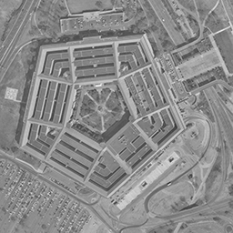
(a)

(b)

(c)

(d)

Figure 3: Some of images used in the experiment (USC-SIPI database [31]): (a) aerial image, (b) misc image, (c) texture image, and (d) sequence image.

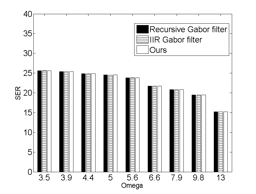
(a) Aerial

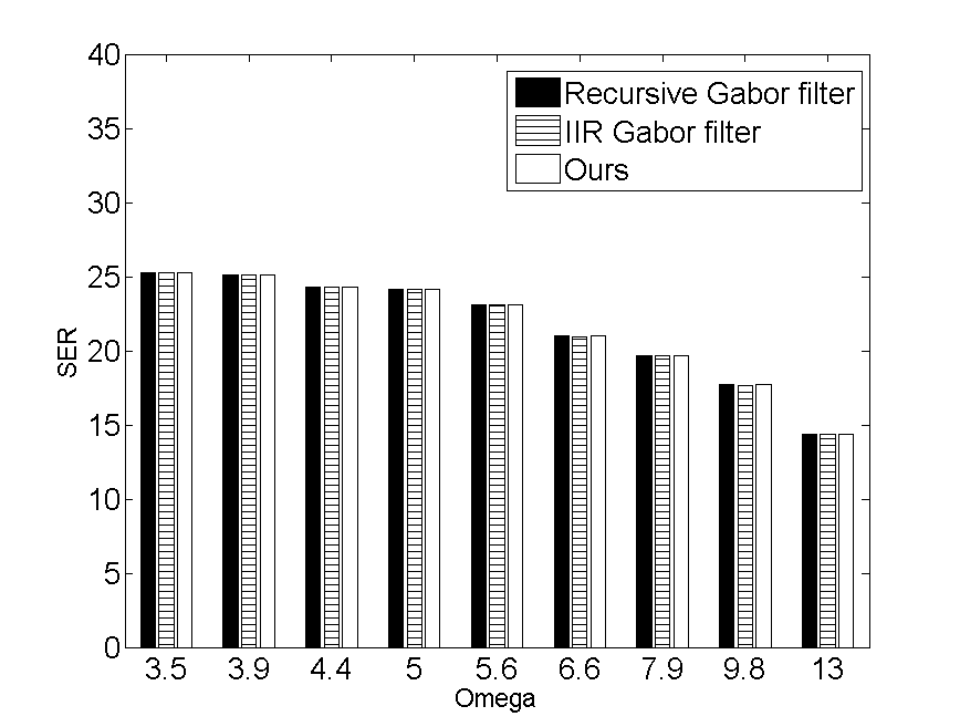
(b) Misc

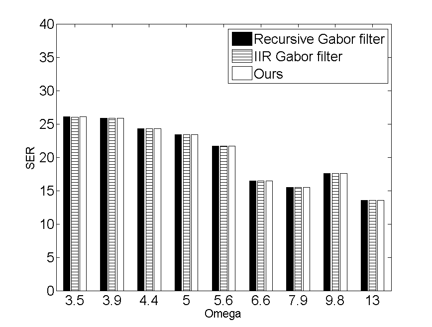
(c) Sequences

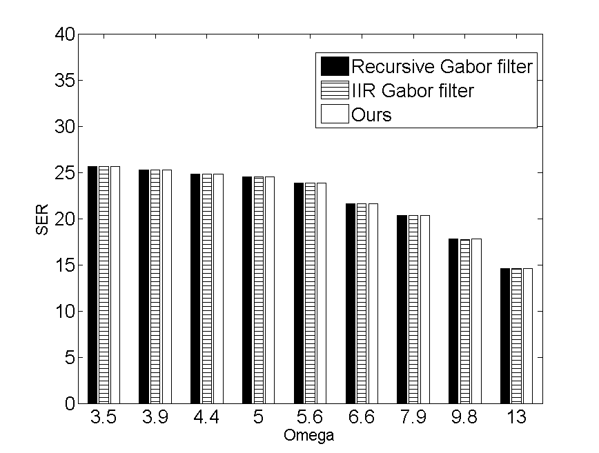
(d) Textures

Figure 4: Objective comparison using the imagery parts of 2-D complex Gabor filtering outputs with the varying frequency $\omega$ when $\theta=\pi/3$. We compared the average SER values of three methods, the recursive Gabor filter [23], IIR Gabor filter [24], and our method, for four datasets: (a) aerial, (b) miscellaneous, (c) sequences, and (d) textures.

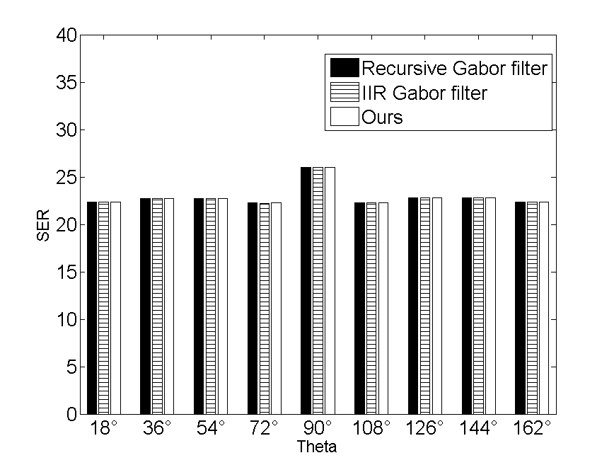
(a) Aerial

(b) Misc

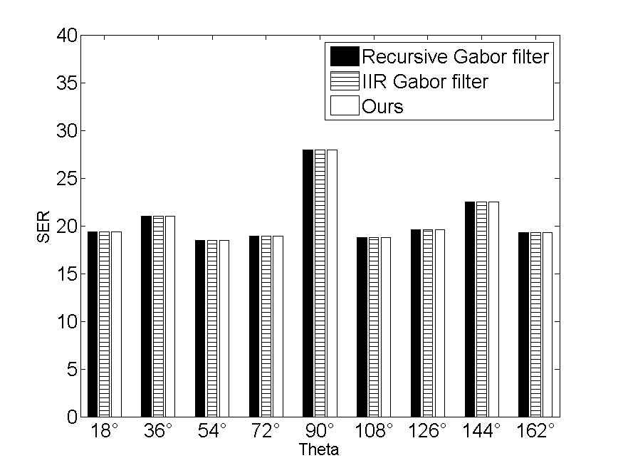
(c) Sequences

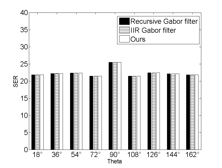
(d) Textures

Figure 5: Objective comparison using the imagery parts of 2-D Gabor filtering outputs with the varying orientation $\theta$ when $\omega=13$. Similar to Fig. 4, the average SER values were measured using the recursive Gabor filter [23], IIR Gabor filter [24], and our method.

IV-B Filtering Quality Comparison

All the fast Gabor filtering methods including ours produce approximated results, as they counts on the recursive Gaussian filtering [30, 25]. In our method, the decomposed 1-D signals are convolved using the recursive Gaussian filtering based on the IIR approximation. The IIR filters run fast at the cost of the filtering quality loss. It was reported in [30, 25] that the quality loss is negligible when using the standard deviation within an appropriate range. We compared the filtering quality with two fast Gabor filtering approaches [23, 24].

We used input images from the USC-SIPI database [31] which consists of four different classes of images: aerial images, miscellaneous images, sequence images, and texture images, some of which are shown in Fig. 3. The filtering quality was measured for the 2-D complex Gabor filter bank only, as the 2-D localized SDFT tends to show similar filtering behaviors. We measured the PSNR by using ground truth results of the lossless FIR Gabor filter in (1), and then computed an objective quality for each of four datasets. The Gabor filtering outputs are in a complex form, so we measured the filtering quality for real and imagery parts, respectively. Also, the filtering outputs do not range from 0 to 255, different from an image. Thus, instead of the peak signal-to-noise ratio (PSNR) widely used in an image quality assessment, we computed the signal-to-error ratio (SER), following [24]:

$$SER[dB]=10\log_{10}\frac{{\sum\limits_{x,y}{\left({{\cal R}\{F(x,y)\}}\right)^{2}}}}{{\sum\limits_{x,y}{\left({{\cal R}\{F(x,y)\}-{\cal R}\{F_{t}(x,y)\}}\right)^{2}}}},\\$$

where $F$ and $F_{t}$ are the Gabor filtering results obtained using the fast method and the lossless FIR filter, respectively. ${\cal R}(F)$ represents the real part of $F$. The SER can also be measured with the imagery part ${\cal I}(F)$. We computed the approximation error for the frequency $\omega\in\{3.5,3.9,...,9.8,13\}$ and the orientation $\theta\in\{18^{\circ},36^{\circ},...,162^{\circ}\}$.

Fig. 4 and 5 compare the objective Gabor filtering quality by measuring the average SER values of the imagery parts with respect to the varying frequency $\omega$ and orientation $\theta$ for four datasets: aerial, miscellaneous, sequences, and textures images. The average SER values are similar to all three methods: the recursive Gabor filter, IIR Gabor filter, and ours. Four different classes of images did not show significantly different tendency in terms of the filtering quality. Fig. 6 and 7 shows the SER values measured using the real parts. Interestingly, the average SER values of the real parts at some frequencies and orientations become lower. It was explained in [24] that the difference between DC values of the lossless FIR and approximated (IIR) filters happens to become larger at these ranges. In Fig. 8, we plotted 1-D profiles using the real parts of Gabor filtering results for two cases with low and high SER values. The horizontal and vertical axes the pixel location and the real part value of the Gabor filtering, respectively. In the case with the low SER value, we found that an overall tendency is somehow preserved with some offsets. Fig. 9 shows the Gabor filtering images obtained from the proposed method. The absolute magnitude was used for visualization. Subjective quality of the results are very similar to that of the original lossless FIR Gabor filtering.

V Conclusion

We have presented a new method for fast computation of the 2-D complex Gabor filter bank at multiple orientations and frequencies. By decomposing the Gabor basis kernels and performing the Gabor filtering in a separable manner, the proposed method achieved a substantial runtime gain by reducing the computational redundancy that exists the 2-D complex Gabor filter bank. This method was further extended into the 2-D localized SDFT that uses the Gaussian kernel to offer the spatial localization ability as in the Gabor filter. The computational gain was verified in both analytic and experimental manners. We also evaluated the filtering quality as the proposed method counts on the recursive Gaussian filtering based on IIR approximation. It was shown that the proposed method maintains a similar level of filtering quality when compared to state-of-the-arts approaches for fast Gabor filtering, but it runs much faster. We believe that the proposed method for the fast 2-D complex Gabor filter bank is crucial to various computer vision tasks that require a low cost computation. Additionally, the 2-D localized SDFT is expected to provide more useful information thanks to the spatial localization property in many tasks based on the frequency analysis, replacing the conventional 2-D SDFT approaches using the simple box kernel. We will continue to study the effectiveness of the 2-D localized SDFT in several computer vision applications as future work.

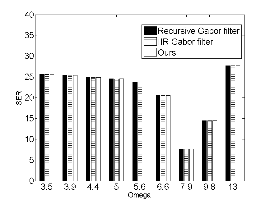
(a) Aerial

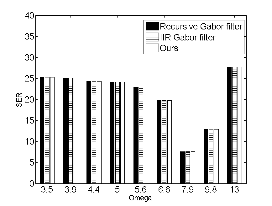
(b) Misc

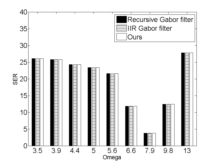
(c) Sequences

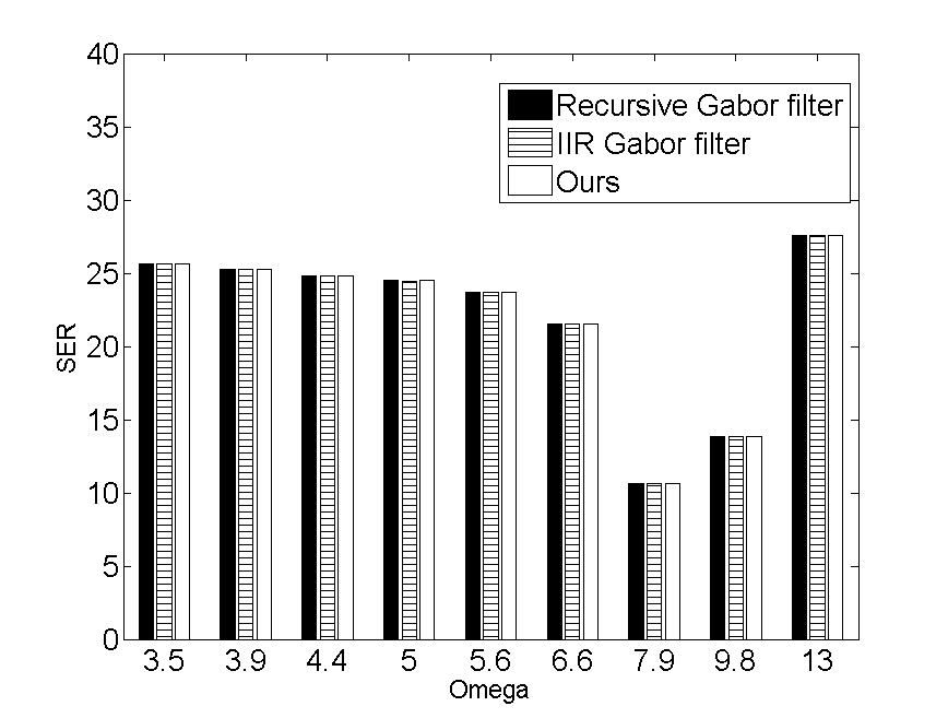
(d) Textures

Figure 6: Objective comparison using the real parts of 2-D complex Gabor filtering outputs with the varying frequency $\omega$ when $\theta=\pi/3$. The SER values were measured in a manner similar to Fig. 4.

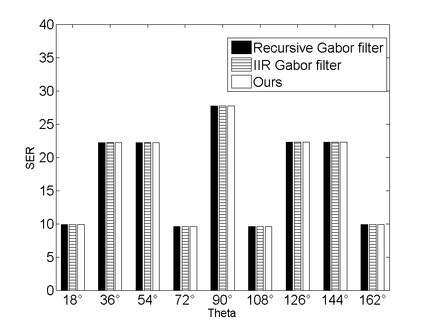
(a) Aerial

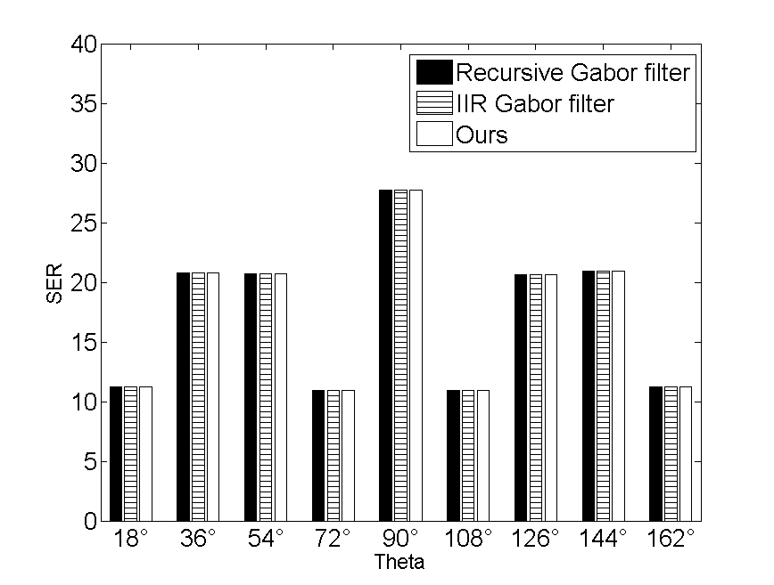
(b) Misc

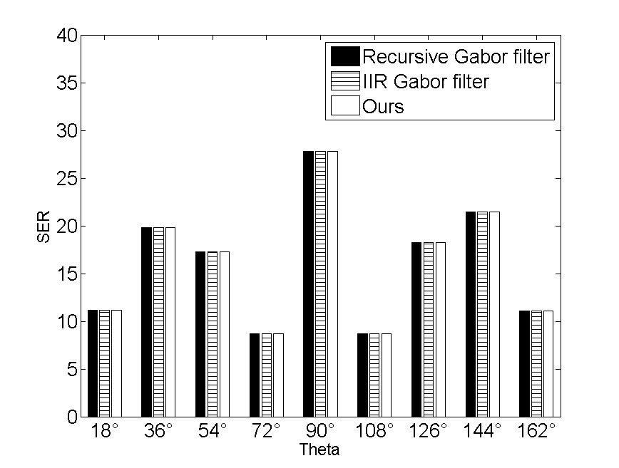
(c) Sequences

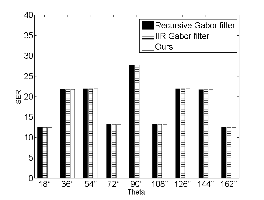
(d) Textures

Figure 7: Objective comparison using the real parts of 2-D complex Gabor filtering outputs with the varying orientation $\theta$ when $\omega=13$. The SER values were measured in a manner similar to Fig. 5.

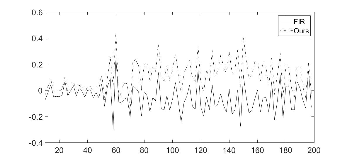
(a)

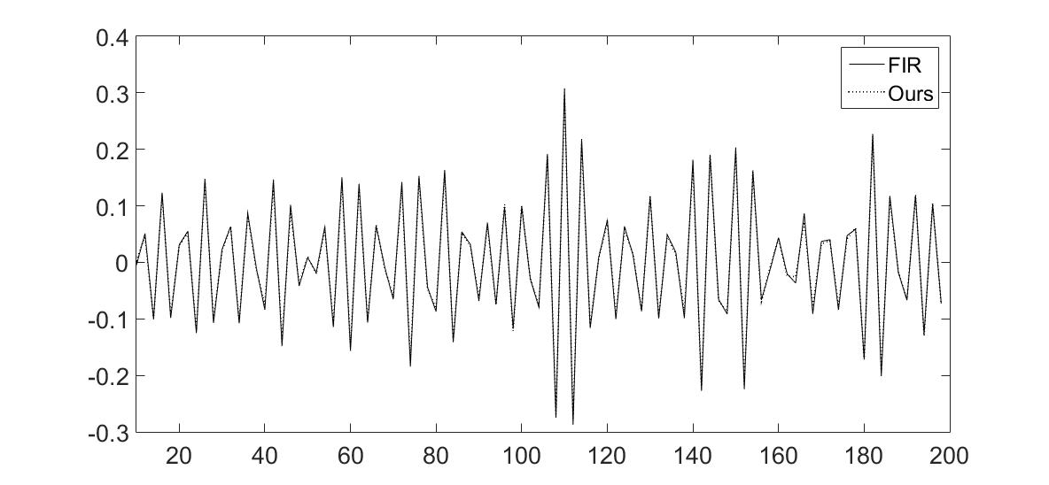
(b)

Figure 8: 1-D profiles of 2-D complex Gabor filtering results: (a) the real part at $\omega=7.9$ and $\theta=\pi/3$ when $SER=10.57$, (b) the real part at $\omega=3.5$ and $\theta=\pi/3$ when $SER=25.61$.

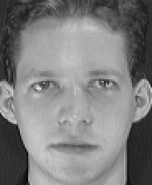
(a) Face image

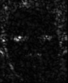
(b) $\sigma=3,\theta=\pi/4$

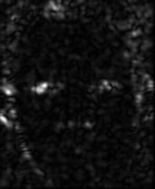
(c) $\sigma=3,\theta=3\pi/4$

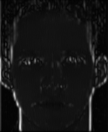
(d) $\sigma=2,\theta=0$

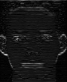
(e) $\sigma=2,\theta=\pi/2$

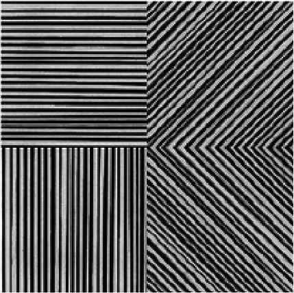
(f) Texture image

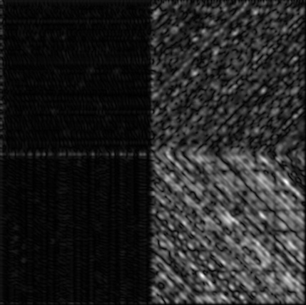
(g) $\sigma=2.7,\theta=\pi/4$

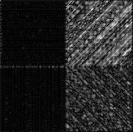
(h) $\sigma=2.7,\theta=3\pi/4$

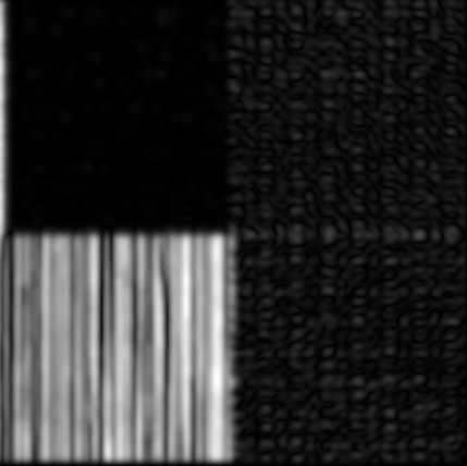
(i) $\sigma=4,\theta=0$

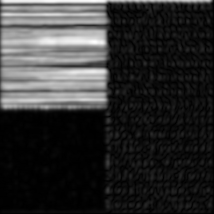
(j) $\sigma=4,\theta=\pi/2$

Figure 9: 2-D complex Gabor filter bank outputs computed by our method: The filtering results are in a complex form, so we visualize them with an absolute magnitude. $\lambda=\sigma/\pi$ depends on $\sigma$.

References

- [1] I. Daubechies, “The wavelet transform, time-frequency localization and signal analysis,” IEEE Trans. Information Theory, vol. 36, no. 5, pp. 961–1005, 1990.
- [2] J. G. Daugman, “Uncertainty relation for resolution in space, spatial frequency, and orientation optimized by two-dimensional visual cortical filters,” The Journal of the Optical Society of America A, vol. 2, no. 7, pp. 1160–1169, 1985.
- [3] L. Shen, L. Bai, and M. C. Fairhurst, “Gabor wavelets and general discriminant analysis for face identification and verification,” Image Vision Comput., vol. 25, no. 5, pp. 553–563, 2007.
- [4] L. Xu, W. Lin, and C.-C. J. Kuo, Visual Quality Assessment by Machine Learning. Springer, 2015.
- [5] J. Kamarainen, V. Kyrki, and H. Kälviäinen, “Invariance properties of gabor filter-based features-overview and applications,” IEEE Trans. Image Processing, vol. 15, no. 5, pp. 1088–1099, 2006.
- [6] T. P. Weldon, W. E. Higgins, and D. F. Dunn, “Efficient gabor filter design for texture segmentation,” Pattern Recognition, vol. 29, no. 12, pp. 2005–2015, 1996.
- [7] F. Bianconi and A. Fernández, “Evaluation of the effects of gabor filter parameters on texture classification,” Pattern Recognition, vol. 40, no. 12, pp. 3325–3335, 2007.
- [8] S. Liao, M. W. K. Law, and A. C. S. Chung, “Dominant local binary patterns for texture classification,” IEEE Trans. Image Processing, vol. 18, no. 5, pp. 1107–1118, 2009.
- [9] C. Li, G. Duan, and F. Zhong, “Rotation invariant texture retrieval considering the scale dependence of gabor wavelet,” IEEE Trans. Image Processing, vol. 24, no. 8, pp. 2344–2354, 2015.
- [10] L. Wiskott, J.-M. Fellous, N. Krüger, and C. von der Malsburg, “Face recognition by elastic bunch graph matching,” IEEE Trans. Pattern Anal. Mach. Intell., vol. 19, no. 7, pp. 775–779, Jul. 1997.
- [11] C. Liu and H. Wechsler, “Independent component analysis of gabor features for face recognition,” IEEE Trans. Neural Networks, vol. 14, no. 4, pp. 919–928, 2003.
- [12] L. Shen and L. Bai, “A review on gabor wavelets for face recognition,” Pattern Anal. Appl., vol. 9, no. 2-3, pp. 273–292, 2006.
- [13] Z. Lei, S. Liao, R. He, M. Pietikäinen, and S. Z. Li, “Gabor volume based local binary pattern for face representation and recognition,” in 8th IEEE International Conference on Automatic Face and Gesture Recognition (FG 2008), Amsterdam, The Netherlands, 17-19 September 2008, 2008, pp. 1–6.
- [14] Y. Cheng, Z. Jin, H. Chen, Y. Zhang, and X. Yin, “A fast and robust face recognition approach combining gabor learned dictionaries and collaborative representation,” Int. J. Machine Learning & Cybernetics, vol. 7, no. 1, pp. 47–52, 2016.
- [15] W. Gu, C. Xiang, Y. V. Venkatesh, D. Huang, and H. Lin, “Facial expression recognition using radial encoding of local gabor features and classifier synthesis,” Pattern Recognition, vol. 45, no. 1, pp. 80–91, 2012.
- [16] M. K. Mandal and A. Awasthi, Understanding Facial Expressions in Communication. Springer, 2015.
- [17] F. Bianconi and A. Fernández, “Fingerprints verification based on their spectrum,” Pattern Recognition, vol. 40, no. 12, pp. 3325–3335, 2007.
- [18] K. He, J. Sun, and X. Tang, “Guided image filtering,” in European Conf. on Computer Vision, 2010, pp. 1–14.
- [19] E. S. L. Gastal and M. M. Oliveira, “Domain transform for edge-aware image and video processing,” ACM Trans. Graph., vol. 30, no. 4, p. 69, 2011.
- [20] D. Min, S. Choi, J. Lu, B. Ham, K. Sohn, and M. N. Do, “Fast global image smoothing based on weighted least squares,” TIP, vol. 23, no. 12, pp. 5638–5653, 2014.
- [21] S. Qiu, F. Zhou, and P. E. Crandall, “Discrete gabor transforms with complexity O (nlogn),” Signal Processing, vol. 77, no. 2, pp. 159–170, 1999.
- [22] O. Nestares, R. F. Navarro, J. Portilla, and A. Tabernero, “Efficient spatial-domain implementation of a multiscale image representation based on gabor functions,” J. Electronic Imaging, vol. 7, no. 1, pp. 166–173, 1998.
- [23] I. T. Young, L. J. van Vliet, and M. van Ginkel, “Recursive gabor filtering,” IEEE Trans. Signal Processing, vol. 50, no. 11, pp. 2798–2805, 2002.
- [24] A. Bernardino and J. Santos-Victor, “Fast IIR isotropic 2-d complex gabor filters with boundary initialization,” IEEE Trans. Image Processing, vol. 15, no. 11, pp. 3338–3348, 2006.
- [25] L. J. van Vliet, I. T. Young, and P. W. Verbeek, “Recursive gaussian derivative filters,” in Fourteenth International Conference on Pattern Recognition, ICPR 1998, Brisbane, Australia, 16-20 August, 1998, 1998, pp. 509–514.
- [26] A. K. Gangwar and A. Joshi, “Local gabor rank pattern (LGRP): A novel descriptor for face representation and recognition,” in 2015 IEEE International Workshop on Information Forensics and Security, WIFS 2015, Roma, Italy, November 16-19, 2015, 2015, pp. 1–6.
- [27] E. Jacobsen and R. Lyons, “The sliding dft,” IEEE Signal Processing Magazine, vol. 20, no. 2, pp. 74–80, 2003.
- [28] ——, “An update to the sliding dft,” IEEE Signal Processing Magazine, vol. 21, no. 1, pp. 110–111, 2004.
- [29] C. Park, “2d discrete fourier transform on sliding windows,” IEEE Trans. Image Processing, vol. 24, no. 3, pp. 901–907, 2015.
- [30] I. T. Young and L. J. van Vliet, “Recursive implementation of the gaussian filter,” Signal Processing, vol. 44, no. 2, pp. 139–151, 1995.
- [31] The Usc-Sipi Image Database. Univ. Southern California and I. P. Institute, http://sipi.usc.edu/services/database.