Quantum Otto engine with exchange coupling in the presence of level degeneracy

Abstract

We consider a quasi-static quantum Otto cycle using two effectively two-level systems with degeneracy in the excited state. The systems are coupled through isotropic exchange interaction of strength $J>0$, in the presence of an external magnetic field $B$ which is varied during the cycle. We prove the positive work condition, and show that level-degeneracy can act as a thermodynamic resource, so that a larger amount of work can be extracted than from the non-degenerate case, both with and without coupling. We also derive an upper bound for the efficiency of the cycle. This bound is the same as derived for a system of coupled spin-1/2 particles [G. Thomas and R. S. Johal, Phys. Rev. E 83, 031135 (2011)] i.e. without degeneracy, and depends only on the control parameters of the Hamiltonian, but is independent of the level degeneracy and the reservoir temperatures.

I Introduction

The study of thermal machines in the quantum regime, is currently under intense investigation. Different quantum working substances may be employed, such as a three-level maser Scovil and Schulz-DuBois (1959), two-level Quan et al. (2007); Kieu (2006); Abe and Okuyama (2011) or multi-level quantum particles Allahverdyan et al. (2008); Uzdin and Kosloff (2014) such as spins Thomas and Johal (2011); Ivanchenko (2015); Altintas and Müstecaplıoğlu (2015); Thomas et al. (2016) and harmonic oscillators Rezek and Kosloff (2006); Roßnagel et al. (2014); Dillenschneider and Lutz (2009); Agarwal and Chaturvedi (2013). This spurt of interest has been due to advances in the technology of micro- and nano-machines, as well as theoretical progress on the connection between thermodynamics and quantum theory Oppenheim et al. (2002); Vedral and Kashefi (2002); Kosloff (2013); Brandão et al. (2013); Gelbwaser-Klimovsky et al. (2015). When the size of the heat engine is reduced, the presence of quantum discreteness, degeneracy, and quantum correlations pose a natural question: whether the principles of thermodynamics that were customarily applied to macroscopic objects, now retain the same form, and if not, what are the consequent modifications? Quantum analogs of classical Otto cycle serve as a testbed to analyze and illustrate various extensions of thermodynamic ideas in the quantum domain Zhang et al. (2007); Wang et al. (2009); Thomas and Johal (2011); Abah et al. (2012); Li et al. (2013); Thomas and Johal (2014); Zhang et al. (2014); Stefanatos (2014); Wu et al. (2014); Hübner et al. (2014); Peña and Muñoz (2015); Ivanchenko (2015); Alecce et al. (2015); Altintas and Müstecaplıoğlu (2015); Wang et al. (2015); Long and Liu (2015); Zheng and Poletti (2015); Jaramillo et al. (2016); Beau et al. (2016); Çakmak et al. (2016); Leggio and Antezza (2016); Manzano et al. (2016); Insinga et al. (2016); Zheng et al. (2016); Karimi and Pekola (2016); Thomas et al. (2016); Chand and Biswas (2017); Newman et al. (2017).

Recently, quantum Otto cycle (QOC) in the quasi-static limit, with two spin-${1}/{2}$ particles coupled by Heisenberg exchange interaction, was shown to exhibit an enhanced efficiency Thomas and Johal (2011). Though the efficiency is naturally limited by Carnot value, a stronger upper bound ($\eta_{\rm ub}$) was found in the presence of coupling. This bound depends on the control parameters in the Hamiltonian, but not on the reservoir temperatures. An analysis of local work and efficiency shows counter-intuitive effects such as locally the flow of heat may be in a direction opposite to the global temperature gradient Thomas and Johal (2011); Huang et al. (2013, 2014). 100% efficiencies have also been reported using negative absolute temperatures of the heat reservoirs Ivanchenko (2015).

In a related study, the efficiency for a system of a spin-$s$ particle coupled to a spin-1/2 particle Altintas and Müstecaplıoğlu (2015) was shown to exceed $\eta_{\rm ub}$, depending on the spin-value $s$. An outstanding question is whether a bound stricter than the Carnot efficiency may also exist for two coupled spins of arbitrary magnitudes $s_{1}$ and $s_{2}$. In this paper, we take a step in this direction by considering two coupled effectively two-level systems, each with a degenerate excited state. Such systems are often studied in quantum and atom optics e.g. atoms with V-configuration Scullybook , where the excited level is very nearly doubly-degenerate. Within quantum thermodynamics, the role of level-degeneracy has been explored using finite-time models of thermal machines Allahverdyan et al. (2008); Kurizki2015n . We show conditions under which work is extractable from such a working medium using a quasi-static QOC. It will be observed that level-degeneracy can act as a thermodynamic resource, helping to extract larger work than the non-degenerate case, both with and without coupling. Somewhat surprisingly, we obtain the same upper bound on the efficiency, $\eta_{\rm ub}$, for the degenerate case also. Thus the presence of degeneracy alters the extracted work, but not the maximal efficiency of a QOC.

The paper is organized as follows. In Section II, we introduce our working substance and the model for QOC. Various stages of the heat cycle and its efficiency are described within a general framework. In Section III, we discuss the positive work condition (PWC) and engine’s efficiency for the non-interacting case. In Section IV, we calculate the work and efficiency for the interacting case and PWC is proved within a certain regime of parameter values. In Section IV.A, we discuss the upper bound to the efficiency which is stricter than the Carnot efficiency. Section V is on further discussion of our results. The final Section VI summarises our main findings. The computation of eigenvalues of the Hamiltonian, the proofs of PWC and of the upper bound are given in the appendices.

II Quantum Otto Cycle

The working substance consists of two particles which are effectively two-level systems such that while the ground state is non-degenerate, the excited state of each is $n^{(i)}$-fold degenerate, $i=1,2$. The particles are coupled by an Heisenberg exchange interaction specified below. The Hamiltonian of the working substance in the first stage of the cycle is given by:

$${\cal H}_{1} \equiv H_{1}+H_{\rm int},$$ (1)

$$= 2B_{1}\left(s_{z}^{(1)}\otimes I+I\otimes s_{z}^{(2)}\right)+8J\overrightarrow{s}^{(1)}.\overrightarrow{s}^{(2)},$$

where $H_{1}$ is the free or local Hamiltonian and $H_{\rm int}$ is the interaction Hamiltonian with $J>0$ as the anti-ferromagnetic exchange constant. $\overrightarrow{s}^{(i)}\equiv\{s^{(i)}_{x},s^{(i)}_{y},s^{(i)}_{z}|i=1,2\}$, are the generalized spin operators for the particles (see Appendix A). For $n^{(i)}=1$, we have two coupled spin-1/2 particles Thomas and Johal (2011). The various stages of the heat cycle are discussed as follows. A schematic of the cycle is shown in Fig. 1.

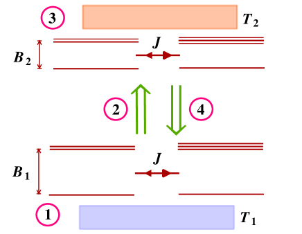
Figure 1: A schematic of QOC between hot ($T_{1}$) and cold ($T_{2}$) heat baths, using working substance as two effectively two-level systems coupled via exchange interaction of strength $J$. The degeneracy of excited levels is $n^{(1)}=2$ and $n^{(2)}=3$. The different stages of the cycle are marked with circles.

Stage 1: The working medium is in thermal equilibrium with a heat reservoir at temperature $T_{1}$. The density matrix $\rho_{1}$ for the working substance is given as:

$$\rho_{1}=\sum_{i=1}^{N}p_{i}{\left|\psi_{i}\right\rangle}{\left\langle\psi_{i}\right|}$$ (2)

where $N=(n^{(1)}+1)(n^{(2)}+1)$ is the number of energy levels with ${\left|\psi_{i}\right\rangle}$ as the corresponding energy eigenstates. $p_{i}=\exp\left(-E_{i}/T_{1}\right)/Z_{1}$ are the occupation probabilities of the microstates with energy levels ($E_{i}$) and $Z_{1}=\sum_{i}\exp\left(-E_{i}/T_{1}\right)$ is the partition function for the system. We set Boltzmann’s constant $k=1$.

Stage 2: The system is isolated from the hot reservoir and the magnetic field is changed from $B_{1}$ to $B_{2}$ such that $B_{2}<B_{1}$. So the local Hamiltonian is then given as: $H_{2}=2B_{2}\left(s_{z}^{(1)}\otimes I+I\otimes s_{z}^{(2)}\right)$. During this process, the quantum adiabatic theorem is assumed to hold Born and Fock (1928), according to which the rate of the process should be slow enough so that the occupation probabilities of the energy levels are maintained. Work is performed by the system during this step.

Stage 3: The system is brought in contact with a cold reservoir at temperature $T_{2}$ ($<T_{1}$). The energy eigenvalues are $E_{i}^{{}^{\prime}}$ and the occupation probabilities change from $p_{i}$ to $p_{i}^{\prime}$ corresponding to canonical density matrix $\rho_{2}$. The amount of heat rejected to the cold reservoir is:

$$Q_{2} = {\rm Tr}[{\cal H}_{2}\Delta\rho],$$ (3)

$$= {\rm Tr}[H_{2}\Delta\rho]+{\rm Tr}[H_{\rm int}\Delta\rho],$$

where $\Delta\rho=(\rho_{1}-\rho_{2})$. The first term above can be identified with the amount of heat locally exchanged by the working substance, while the second term is solely due to the interaction.

Stage 4: The system is detached from the cold reservoir and the magnetic field is increased from $B_{2}$ to $B_{1}$ with occupation probabilities remaining unchanged at $p_{i}^{\prime}$ and energy eigenvalues change from $E_{i}^{{}^{\prime}}$ to $E_{i}$. Work is performed on the system.

Finally the system is attached to the hot reservoir again. Thus the system returns to the initial state, completing the heat cycle. The amount of heat absorbed from the hot reservoir in one cycle is:

$$Q_{1} = {\rm Tr}[{\cal H}_{1}\Delta\rho],$$ (4)

$$= {\rm Tr}[H_{1}\Delta\rho]+{\rm Tr}[H_{\rm int}\Delta\rho],$$

The work performed per cycle is:

$$W=Q_{1}-Q_{2}={\rm Tr}[(H_{1}-H_{2})\Delta\rho].$$ (5)

The efficiency $\eta=W/Q_{h}$ can be written as:

$$\eta = \left(1-\frac{{\rm Tr}[H_{2}\Delta\rho]}{{\rm Tr}[H_{1}\Delta\rho]}\right)\left(1+\frac{{\rm Tr}[H_{\rm int}\Delta\rho]}{{\rm Tr}[H_{1}\Delta\rho]}\right)^{-1},$$ (6)

$$= \eta_{\rm loc}\left(1+\frac{{\rm Tr}[H_{\rm int}\Delta\rho]}{{\rm Tr}[H_{1}\Delta\rho]}\right)^{-1}.$$

The first factor, $\eta_{\rm loc}$, based on the amounts of heat exchanged locally with the system, can be regarded as the efficiency in a local sense. This factor also becomes equal to the efficiency of the engine when the interactions are absent.

In this paper, we are considering the Hamiltonian for which we can write $H_{1}\equiv 2B_{1}h_{0}$, $H_{2}\equiv 2B_{2}h_{0}$, i.e. the free Hamiltonian is proportional to the control parameter $B$, and $H_{\rm int}\equiv 8Jh_{\rm int}$, where $J$ is held fixed. Then we have, $W=2(B_{1}-B_{2}){\rm Tr}[h_{0}\Delta\rho]$. In this case,

$$\eta_{\rm loc}=1-\frac{B_{2}}{B_{1}}=\eta_{0},$$ (7)

where $\eta_{0}$ is the efficiency in the absence of the interaction Comment2 .

Further, as locally the system works like an engine, so ${\rm Tr}[H_{1}\Delta\rho]>0$. From Eq. (6), if ${\rm Tr}[H_{\rm int}\Delta\rho]>0$, then the efficiency is less than the uncoupled case. In this paper, we are interested in the situation ${\rm Tr}[H_{\rm int}\Delta\rho]<0$, whereby the efficiency becomes greater than $\eta_{\rm loc}$, or $\eta_{0}$ Comment . For convenience, we write Eq. (6) as follows:

$$\eta=\eta_{\rm 0}\left(1-\frac{4JY}{B_{1}X}\right)^{-1},$$ (8)

where $X={\rm Tr}[h_{0}\Delta\rho]>0$ and $Y=-{\rm Tr}[h_{\rm int}\Delta\rho]>0$. Now, under certain conditions, it can be proved that $X>Y$. This ensures that an upper bound exists for the efficiency, given as:

$$\eta\leq\eta_{0}\left(1-\frac{4J}{B_{1}}\right)^{-1}.$$ (9)

This bound is independent of the reservoir temperatures, and is tighter than the Carnot limit, within a certain range of parameter values. In Ref. Thomas and Johal (2011), the above bound was proved for the working substance of two coupled spin-1/2 systems. In the following, we make a detailed analysis of work and efficiency in a QOC with our chosen working substance.

III The uncoupled model

We first summarise the cycle in the non-interacting case. The working substance consists of two non-interacting particles in the presence of an externally applied magnetic field $B$ along $z$- axis such that each particle effectively has two energy levels with a non-degenerate ground state, but the excited state may have an arbitrary degeneracy $n^{(1)}$ and $n^{(2)}$, respectively. The Hamiltonian of this system is $H_{1}$. Since the particles are non-interacting, each particle undergoes an independent heat cycle. For a particle with degeneracy $n^{(i)}$, the probabilities at Stage 1 are: $p_{1}=e^{B_{1}/T_{1}}/z_{1}$ and $p_{2}=n^{(i)}e^{-B_{1}/T_{1}}/z_{1}$, where $z_{1}=e^{B_{1}/T_{1}}+n^{(i)}e^{-B_{1}/T_{1}}$. Similarly, the occupation probabilities at Stage 3 are: ${p_{1}^{\prime}=e^{B_{2}/T_{2}}/z_{2}}$ and ${p_{2}^{\prime}=n^{(i)}e^{-B_{2}/T_{2}}/z_{2}}$, where $z_{2}=e^{B_{2}/T_{2}}+n^{(i)}e^{-B_{2}/T_{2}}$. Then the heat absorbed from the hot reservoir is: $q_{1}=2B_{1}\left(p_{2}-p_{2}^{\prime}\right)$, and the heat rejected to cold reservoir is: $q_{2}=2B_{2}\left(p_{2}-p_{2}^{\prime}\right)$. The work extracted per particle during the heat cycle is

$$w=q_{1}-q_{2}=2(B_{1}-B_{2})\left(p_{2}-p_{2}^{\prime}\right).$$ (10)

Since $B_{1}>B_{2}$, so for a positive work condition (PWC), we must have $p_{2}>p_{2}^{\prime}$, which means

$$\frac{B_{2}}{T_{2}}>\frac{B_{1}}{T_{1}}.$$ (11)

As shown in Appendix B, the extracted work from such a system with $n^{(i)}$-fold degeneracy, is bounded from above by the work from $n^{(i)}$ two-level systems (without degeneracy). Thus degeneracy can act as a thermodynamic resource.

The efficiency $\eta_{0}={w}/{q_{1}}$, is given by $1-{B_{2}}/{B_{1}}$. Due to (11), the engine efficiency satisfies:

$$\eta_{0}=1-\frac{B_{2}}{B_{1}}<1-\frac{T_{2}}{T_{1}}=\eta_{C},$$ (12)

where $\eta_{C}$ is the Carnot efficiency.

IV The coupled model

We now switch on the coupling between the particles. The Hamiltonian of this system for $B=B_{1}$ is as given in Eq. 1. The eigenvalues of the Hamiltonian (see Appendix A for an example with particular values of degeneracies), ordered in increasing energy, are as follows:

$$\begin{array}[]{l l}{\rm Energy}\;(E_{i})&{\rm Degeneracy}\;(g_{i})\\ -2B_{1}+2J&1\\ -6J&1\\ -2J&n^{(1)}+n^{(2)}-2\equiv m\\ +2J&1\\ +2B_{1}+2J&n^{(1)}n^{(2)}\equiv n\end{array}$$

We take parameter $J$ to satisfy $B>4J$, so that $-2B+2J$ is the ground state. In this paper, we study the effect of coupling strength $J$ on thermodynamic properties of QOC, for given values of $B_{1},B_{2},T_{1}$ and $T_{2}$. Now the occupation probabilities for the above energy levels can be calculated as: $P_{i}={g_{i}e^{-E_{i}/T}}/{\sum_{i}g_{i}e^{-E_{i}/T}}$. We denote the probabilities at Stage 1 by $P_{i}$ with $B=B_{1}$ and temperature $T_{1}$, and that at Stage 3 by $P_{i}^{{}^{\prime}}$ with $B=B_{2}$ and temperature $T_{2}$. Note that for the simplest case of two spin-1/2 particles where $n^{(1)}=n^{(2)}=1$, we have only four distinct energy levels—without degeneracy. Further, the parameter values satisfy Eq. (11).

Now, the heat absorbed by the working medium during Stage 1, and the heat rejected to the sink during Stage 3 respectively is:

$$Q_{1}=2B_{1}X-8JY,\quad Q_{2}=2B_{2}X-8JY,$$ (13)

where

$$X = P_{1}^{{}^{\prime}}-P_{1}+P_{5}-P_{5}^{{}^{\prime}},$$ (14)

$$Y = P_{2}-P_{2}^{{}^{\prime}}+\frac{1}{2}(P_{3}-P_{3}^{{}^{\prime}}).$$ (15)

The work performed in one cycle is:

$$W=Q_{1}-Q_{2}=2(B_{1}-B_{2})X.$$ (16)

Then as shown in Appendix B, the PWC i.e. $W>0$ holds as long as $J\leq J_{c}$, where

$$J_{c}=\frac{1}{4}{\left(\frac{1}{T_{2}}-\frac{1}{T_{1}}\right)^{-1}}\left({\frac{B_{2}}{T_{2}}-\frac{B_{1}}{T_{1}}}\right).$$ (17)

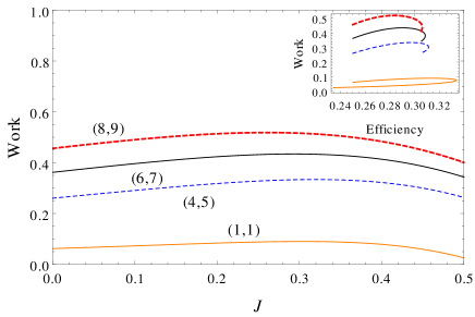
Figure 2: The work extracted from the engine as a function of the coupling strength $J$ for different $(n^{(1)},n^{(2)})$. The parameter values are $B_{1}$=4, $B_{2}$=3, $T_{1}=2$ and $T_{2}=1$. The inset shows the corresponding parametric plots of work versus efficiency as function of parameter $J\in[0,J_{c}]$, traced in a clockwise fashion. The loop-shaped curves show that work and efficiency achieve their maximum values at different values of $J$.

In other words, for given values $B_{1},B_{2},T_{1}$ and $T_{2}$, satisfying Eq. (11), a sufficient criterion for $W>0$ in the coupled case is that $J\leq J_{c}$. In Fig. 2, it is shown that degeneracy of the excited level leads to a higher work extraction.

IV.1 Efficiency and its upper bound

Now, from Eq. (8), if $J=0$, the efficiency is equal to $\eta_{0}$. It is observed that $Y(J)$ as function of $J$ shows a non-monotonic behavior, so that $\eta$ first increases with $J$, but then decreases, and beyond a certain $J(\equiv J_{m})$, becomes less than $\eta_{0}$, (see Fig. 3). Within the general discussion of Section II, we can say that the efficiency is equal to $\eta_{0}$ when ${\rm Tr}[H_{\rm int}\Delta\rho]=0$. This happens in the case of no interactions, $J=0$, but may have a solution for some non-zero interaction strength. At the latter point, we have then the condition ${\rm Tr}[H_{\rm int}\rho_{1}]={\rm Tr}[H_{\rm int}\rho_{2}]$, i.e. the average interaction energy is not altered on changing the equilibrium state of the working substance from state $\rho_{1}$ to $\rho_{2}$.

So $J_{m}$ is determined by $Y(J_{m})=0$. This implies, from Eq. (15), $P_{3}+2P_{2}=P_{3}^{\prime}+2P_{2}^{\prime}$. Expressing $P_{3}$ ($P_{3}^{\prime}$) in terms of $P_{2}$ ($P_{2}^{\prime}$), this condition is rewritten as:

$$(me^{-4J_{m}/T_{1}}+1)P_{2}=(me^{-4J_{m}/T_{2}}+1)P_{2}^{\prime}.$$ (18)

First, we take the case of two spin-1/2 particles ($m=0$). Then $P_{2}=P_{2}^{\prime}$ is the condition for $Y(J_{0})=0$. In this case, we can explicitly solve for $J_{0}$:

$$J_{0}=\frac{1}{8}\left(\frac{1}{T_{2}}-\frac{1}{T_{1}}\right)^{-1}\ln\left(\frac{1+e^{2B_{2}/T_{2}}+e^{-2B_{2}/T_{2}}}{1+e^{2B_{1}/T_{1}}+e^{-2B_{1}/T_{1}}}\right).$$ (19)

For the above case, it can be shown that $J_{0}\leq J_{c}$, the equality being approached for low temperatures. However, in the case of degeneracy ($m\neq 0$), it is not possible to find a closed expression for $J_{m}$. Numeric evidence shows that degeneracy ($m\neq 0$) may lead to an extended regime of enhanced efficiency, beyond $J=J_{c}$ values (see Fig. 3).

For the uncoupled or $J=0$ case, PWC leads to condition $p_{2}>p_{2}^{\prime}$. As $J$ becomes non-zero, we have $P_{2}>P_{2}^{\prime}$ up to a certain value of $J$, after which the opposite condition i.e. $P_{2}^{\prime}>P_{2}$, holds. It is convenient to do further analysis in the following regimes, separately: (i) $P_{2}>P_{2}^{\prime}$, (ii) $P_{2}^{\prime}>P_{2}$ (see inset of Fig. 3).

(i) $P_{2}>P_{2}^{\prime}$ Regime: It can be shown (Appendix C) that the condition $P_{2}>P_{2}^{\prime}$ implies the following relations between the occupation probabilities:

$$P_{1}<P_{1}^{{}^{\prime}}\quad P_{3}>P_{3}^{{}^{\prime}},\quad P_{4}>P_{4}^{{}^{\prime}},\quad P_{5}>P_{5}^{{}^{\prime}}.$$ (20)

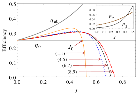
Figure 3: The variation of efficiency of the engine as a function of the coupling strength $J$, for different $(n^{(1)},n^{(2)})$. The parameter values are $B_{1}$=4, $B_{2}$=3, $T_{1}=2$ and $T_{2}=1$. $J_{0}$ marks the value of $J$ where efficiency for (1,1) case (without degeneracy) cuts the uncoupled efficiency line, $\eta_{0}=0.25$. Upper bound $\eta_{\rm ub}$ is also shown. The inset shows the regimes $P_{2}>P_{2}^{\prime}$ and $P_{2}^{\prime}>P_{2}$ vs. $J$ for (4,5) case; the curves for probabilites cross each other at a value of $J<J_{c}=0.5$.

PWC has already been proved, but here due to $P_{5}>P_{5}^{{}^{\prime}}$ and $P_{1}<P_{1}^{{}^{\prime}}$, it is clear that $X>0$, or $W>0$. From Eqs. (13) and (16), the efficiency of the engine in the general case is:

$$\eta=\frac{\left(B_{1}-B_{2}\right)X}{B_{1}X-4JY}={\eta_{0}}{\left(1-\frac{4JY}{B_{1}X}\right)^{-1}}.$$ (21)

Further, in this regime, due to Eq. (20), we also have $Y>0$, which implies that the efficiency, Eq. (21), is higher than uncoupled case: $\eta>\eta_{0}$. Further, it can be proved (Appendix C) that $X>Y$. Therefore, we can write:

$$\eta\leq{\eta_{0}}\left({1-\frac{4J}{B_{1}}}\right)^{-1}\equiv\eta_{\rm ub}.$$

(ii) $P_{2}^{\prime}>P_{2}$ Regime: Now, we have seen that $Y>0$ is a necessary condition for $\eta>\eta_{0}$. So from Eq. (15), when $P_{2}^{\prime}>P_{2}$, then in order to have an enhancement of efficiency, we must have $P_{3}>P_{3}^{\prime}$. Then we also obtain $P_{4}>P_{4}^{{}^{\prime}}$ and $P_{5}>P_{5}^{{}^{\prime}}$. Note that this still leaves the inequality between $P_{1}$ and $P_{1}^{\prime}$ undetermined. However, it can be shown here also that $X>Y$ (Appendix C) and so the same upper bound on efficiency holds in this regime also.

Finally, it can be directly seen that the upper bound $\eta_{\rm ub}$ derived above is less than the Carnot limit $\eta_{C}$, as long as $J<J_{c}$, where $\eta_{\rm ub}=\eta_{C}$, for $J=J_{c}$.

V Discussion

In an earlier study Allahverdyan et al. (2008), and more recently Kurizki2015n , level degeneracy has been shown to act as a thermodynamic resource. In Ref. Allahverdyan et al. (2008), a two-step, finite time cycle was considered using two multilevel systems, each in contact with its respective reservoir. The working medium is regarded as isolated from the reservoirs during the work extraction step. However, in Ref. Kurizki2015n , the working medium— in the form of a V-configuration system, is continuously coupled to both the reservoirs during the cycle. In the present work, using a quasi-static, four-step Otto cycle on such systems, it is shown that degeneracy can act as a thermodynamic resource and the work ($w_{n}$) extracted from a two-level system with $n$-fold degeneracy in the excited level, is bounded from above by the work ($w_{1}$) obtained from $n$ two-level systems, i.e. $w_{n}\leq nw_{1}$ (see Appendix B). For the special case of a V-configuration system, it implies $w_{2}\leq 2w_{1}$. This result may be compared to an analogous result on the power extracted in case of a finite-time model Kurizki2015n using the same system. By the same token, the work per cycle from two non-interacting V-configuration systems would be bounded by the work from four two-level systems. However, as we show by numerical evidence in Fig. 4, the presence of the exchange coupling between two V-configuration systems may lead to a higher amount of extracted work than from four two-level systems.

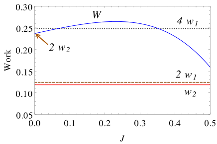
Figure 4: The extracted work ($W$) in a QOC with two interacting V-configuration systems ($n^{(1)}=n^{(2)}=2$) as a function of $J$, compared with two such non-interacting systems ($2w_{2}$), as well as four non-interacting two-level systems ($4w_{1}$). The lines showing $w_{2}<2w_{1}$ illustrate that $w_{n}$ is bounded by $nw_{1}$ (see Appendix B). The parameter values are set at $B_{1}$=4, $B_{2}$=3, $T_{1}=2.5$ and $T_{2}=1.25$.

VI Summary

We analyzed quantum Otto engine between two heat reservoirs, using two effectively two-level particles with degeneracy in the excited state. In our model, the particles are coupled by isotropic exchange interaction in the presence of an external magnetic field $B$, varied during the cycle. We could show that for given values of $B_{1},B_{2},T_{1}$ and $T_{2}$, satisfying ${B_{2}}/{T_{2}}>{B_{1}}/{T_{1}}$ (PWC for the uncoupled case), a sufficient criterion for $W>0$ in the coupled case is that $J\leq J_{c}$ where $J_{c}$ is a certain critical value (independent of degeneracy). It is shown that coupling can lead to enhancement in both the extracted work and the efficiency. An upper bound to the efficiency is derived in the regime $J<J_{c}$, which also implies that the bound itself is limited by Carnot value. Interestingly, the bound is independent of the degeneracy of the levels and is thus equal to the one found for two coupled spin-1/2 particles Thomas and Johal (2011). On the other hand, we find that degeneracy can act as thermodynamic resource, helping to extract a larger amount of work, with or without coupling. Further, numerical evidence shows that the degeneracy ($m\neq 0$) leads to an enhancement of work and efficiency even in the strong coupling regime ($J>J_{c}$). A corresponding analysis in this regime could shed more light on the role of degeneracy in the performance of the idealized cycle.

Appendix A Generalized spin operators and the Hamiltonian

In the main text, we assumed arbitrary values for the degeneracies of excited states of the two particles. In the following, we calculate the eigenvalues of the Hamiltonian for a particular example: when one particle has a non-degenerate ground state and a two-fold degenerate excited state ($n^{(1)}=2$), while the other particle has four energy levels with one ground state and the excited state as three-fold degenerate ($n^{(2)}=3$). Therefore, we have $m=n^{(1)}+n^{(2)}-2=3$, and $n=n^{(1)}n^{(2)}=6$. For the first particle, the operator $s_{z}^{\left(1\right)}$ is written as:

$$s_{z}^{\left(1\right)}=\frac{1}{2}\left(\begin{array}[]{ccr}{1}&{0}&{0}\\ {0}&{1}&{0}\\ {0}&{0}&{-1}\end{array}\right),$$

where Planck’s constant has been set to unity. The normalized eigenstates of $s_{z}^{\left(1\right)}$:

$$\left(\begin{array}[]{l}{1}\\ {0}\\ {0}\end{array}\right),\left(\begin{array}[]{l}{0}\\ {1}\\ {0}\end{array}\right),\left(\begin{array}[]{l}{0}\\ {0}\\ {1}\end{array}\right)$$

denoted as $\left|+\right\rangle,\left|0\right\rangle,\left|-\right\rangle$, corresponding to eigenvalues $1/2,1/2,-1/2$ respectively.

We define the raising operator as : $s_{+}^{\left(1\right)}={|\alpha\rangle}\langle-|$, where $|\alpha\rangle=({|+\rangle}+{|0\rangle})/{\sqrt{2}}$. This implies that the action of $s_{+}^{\left(1\right)}$ on $|-\rangle$ takes the particle into a superposition of the two (degenerate) excited states, with equal amplitudes ($1\sqrt{2}$). In matrix form, we obtain

$$s_{+}^{\left(1\right)}=\frac{1}{\sqrt{2}}\left(\begin{array}[]{ccc}{0}&{0}&{1}\\ {0}&{0}&{1}\\ {0}&{0}&{0}\end{array}\right).$$

The lowering operator defined as $s_{-}^{(1)}=\left(s_{+}^{(1)}\right)^{{\dagger}}$, is given by:

$$s_{-}^{(1)}=\frac{1}{\sqrt{2}}\left(\begin{array}[]{ccc}{0}&{0}&{0}\\ {0}&{0}&{0}\\ {1}&{1}&{0}\end{array}\right).$$

The operators $s_{x}^{\left(1\right)}=(s_{+}^{(1)}+s_{-}^{(1)})/2$ and $s_{y}^{\left(1\right)}=({s_{+}^{(1)}-s_{-}^{(1)}})/{2i}$ are given as:

$$s_{x}^{\left(1\right)}=\frac{1}{2\sqrt{2}}\left(\begin{array}[]{ccc}{0}&{0}&{1}\\ {0}&{0}&{1}\\ {1}&{1}&{0}\end{array}\right),\quad s_{y}^{\left(1\right)}=\frac{1}{2\sqrt{2}i}\left(\begin{array}[]{rrr}{0}&{0}&{1}\\ {0}&{0}&{1}\\ {-1}&{-1}&{0}\end{array}\right).$$

The particle operators for the other particle with one ground state and the excited state is 3-fold degenerate, are similarly calculated and given as follows.

$$s_{z}^{\left(2\right)}=\frac{1}{2}\left(\begin{array}[]{cccc}{1}&{0}&{0}&{0}\\ {0}&{1}&{0}&{0}\\ {0}&{0}&{1}&{0}\\ {0}&{0}&{0}&{-1}\end{array}\right),$$

and

$$s_{x}^{\left(2\right)}=\frac{1}{2\sqrt{3}}\left(\begin{array}[]{cccc}{0}&{0}&{0}&{1}\\ {0}&{0}&{0}&{1}\\ {0}&{0}&{0}&{1}\\ {1}&{1}&{1}&{0}\end{array}\right),s_{y}^{\left(2\right)}=\frac{1}{2\sqrt{3}i}\left(\begin{array}[]{rrrc}{0}&{0}&{0}&{1}\\ {0}&{0}&{0}&{1}\\ {0}&{0}&{0}&{1}\\ {-1}&{-1}&{-1}&{0}\end{array}\right).$$

Then the eigenvalues of the Hamiltonian

$${\cal H}_{1} = 2B_{1}(s_{z}^{(1)}\otimes I+I\otimes s_{z}^{(2)})$$

$$+8J(s_{x}^{(1)}\otimes s_{x}^{(2)}+s_{y}^{(1)}\otimes s_{y}^{(2)}+s_{z}^{(1)}\otimes s_{z}^{(2)}),$$

are computed to be:

$$\begin{array}[]{r c}{\rm Energy}\;(E_{i})&{\rm Degeneracy}\;(g_{i})\\ -2B_{1}+2J&1\\ -6J&1\\ -2J&3\\ +2J&1\\ 2B_{1}+2J&6\end{array}$$

Appendix B Degeneracy as a Thermodynamic Resource

The work extracted from the $n$-fold degenerate system is given by

$$w_{n}=2n(B_{1}-B_{2})\left(\frac{1}{e^{2B_{1}/T_{1}}+n}-\frac{1}{e^{2B_{2}/T_{2}}+n}\right).$$ (22)

Let $w_{1}$ represent the work extracted from a non-degenerate two-level system. In the following, we denote $e^{2B_{1}/T_{1}}=x_{1}$ and $e^{2B_{2}/T_{2}}=x_{2}$. We can write:

$$w_{n}-nw_{1} = 2(B_{1}-B_{2})C^{-1}(x_{2}-x_{1})\times$$ (23)

$$\left[n(1-n^{2})+n(1-n)(x_{1}+x_{2})\right],$$

where $C=(x_{1}+1)(x_{1}+n)(x_{2}+1)(x_{2}+n)>0$. Since $B_{1}>B_{2}$ and $x_{2}>x_{1}$, we note that

$$w_{n}-nw_{1}\leq 0.$$ (24)

Thus the work per cycle from the $n$-fold degenerate system is bounded from above by the work from a working medium of $n$ non-degenerate, two-level systems.

Appendix C Positive Work Condition (PWC)

The work extracted per cycle in the coupled case is given by:

$$W=2(B_{1}-B_{2})\left(P_{1}^{{}^{\prime}}-P_{1}+P_{5}-P_{5}^{{}^{\prime}}\right).$$

Since $B_{1}>B_{2}$ so we need to show $P_{1}^{{}^{\prime}}-P_{1}+P_{5}-P_{5}^{{}^{\prime}}>0$, or $P_{1}^{{}^{\prime}}-P_{5}^{{}^{\prime}}>P_{1}-P_{5}$. This implies

$$Z_{2}^{-1}{(e^{2B_{2}/T_{2}}-ne^{-2B_{2}/T_{2}})}>Z_{1}^{-1}{(e^{2B_{1}/T_{1}}-ne^{-2B_{1}/T_{1}})}.$$

On cross multiplying and rearranging terms, the above inequality can be written as:

$$\begin{array}[]{l}(e^{2B_{2}/T_{2}}-e^{2B_{1}/T_{1}})\\ +2n(e^{-2B_{1}/T_{1}+2B_{2}/T_{2}}-e^{2B_{1}/T_{1}-2B_{2}/T_{2}})\\ +n(e^{-2B_{1}/T_{1}}-e^{-2B_{2}/T_{2}})\\ +mn(e^{-2B_{1}/T_{1}+4J/T_{2}}-e^{-2B_{2}/T_{2}+4J/T_{1}})\\ +n(e^{-2B_{1}/T_{1}+8J/T_{2}}-e^{-2B_{2}/T_{2}+8J/T_{1}})\\ +{m(e^{2B_{2}/T_{2}+4J/T_{1}}-e^{2B_{1}/T_{1}+4J/T_{2}})}\\ +(e^{2B_{2}/T_{2}+8J/T_{1}}-e^{2B_{1}/T_{1}+8J/T_{2}})>0.\end{array}$$

We can check that for $T_{1}>T_{2}$, every term enclosed by parentheses is positive, if we apply the following conditions:

• $\frac{B_{2}}{T_{2}}>\frac{B_{1}}{T_{1}}$,

• $J\leq J_{c}=\frac{1}{4}\left(\frac{1}{T_{2}}-\frac{1}{T_{1}}\right)^{-1}\left(\frac{B_{2}}{T_{2}}-\frac{B_{1}}{T_{1}}\right)$.

The above set of conditions are sufficient to ensure the PWC.

Appendix D Proof of upper bound for the efficiency

D.1 $P_{2}>P_{2}^{{}^{\prime}}$

We assume the inequality: $P_{2}>P_{2}^{{}^{\prime}}$. From the definitions of the probabilites, we can write $P_{3}=me^{-4J/T_{1}}P_{2}$, and $P_{3}^{{}^{\prime}}=me^{-4J/T_{2}}P_{2}^{{}^{\prime}}$. For $T_{1}>T_{2}$ and $J>0$, this implies $P_{3}>P_{3}^{{}^{\prime}}$. Further, due to $P_{4}=e^{-8J/T_{1}}P_{2}$ and $P_{4}^{{}^{\prime}}=e^{-8J/T_{2}}P_{2}^{{}^{\prime}}$, it follows that $P_{4}>P_{4}^{{}^{\prime}}$. Finally, as $P_{5}=ne^{-(2B_{1}/T_{1}+8J/T_{1})}P_{2}$, and $P_{5}^{{}^{\prime}}=ne^{-(2B_{2}/T_{2}+8J/T_{2})}P_{2}^{{}^{\prime}}$, so $P_{5}>P_{5}^{{}^{\prime}}$. Using the normalization condition on probabilites, $\sum_{i=1}^{5}P_{i}=\sum_{i=1}^{5}P_{i}^{\prime}=1$, we finally obtain: $P_{1}<P_{1}^{{}^{\prime}}$. Thus if $P_{2}>P_{2}^{\prime}$ is true, then definite inequalities exist between all the primed and unprimed probabilites:

$$P_{1}^{{}^{\prime}}>P_{1},\quad P_{3}>P_{3}^{{}^{\prime}},\quad P_{4}>P_{4}^{{}^{\prime}},\quad P_{5}>P_{5}^{{}^{\prime}}.$$ (25)

From the above relations, we see that $Y>0$, i.e. the efficiency is higher than $\eta_{0}$. Then we need to show, in Eq. (21), that $X>Y$, i.e.

$$X-Y=P_{1}^{{}^{\prime}}-P_{1}-P_{5}^{{}^{\prime}}+P_{5}+P_{2}^{{}^{\prime}}-P_{2}+\frac{1}{2}(P_{3}^{{}^{\prime}}-P_{3})>0.$$ (26)

From the normalization condition, and the fact that $P_{4}>P_{4}^{{}^{\prime}}$, we can write $P_{1}+P_{2}+P_{3}+P_{5}<P_{1}^{{}^{\prime}}+P_{2}^{{}^{\prime}}+P_{3}^{{}^{\prime}}+P_{5}^{{}^{\prime}}$, or upon rearranging

$$P_{1}^{{}^{\prime}}-P_{1}+P_{2}^{{}^{\prime}}-P_{2}+P_{3}^{{}^{\prime}}-P_{3}+P_{5}^{{}^{\prime}}-P_{5}>0.$$ (27)

As $P_{5}>P_{5}^{{}^{\prime}}$, so if we substitute in Eq. (27), $P_{5}-P_{5}^{{}^{\prime}}>0$ in place of $P_{5}^{{}^{\prime}}-P_{5}$, the resulting expression is still positive. Thus

$$P_{1}^{{}^{\prime}}-P_{1}+P_{5}-P_{5}^{{}^{\prime}}+P_{2}^{{}^{\prime}}-P_{2}+P_{3}^{{}^{\prime}}-P_{3}>0.$$ (28)

Also, using the fact that $P_{3}^{{}^{\prime}}-P_{3}<0$, inequality (28) also implies:

$$P_{1}^{{}^{\prime}}-P_{1}+P_{5}-P_{5}^{{}^{\prime}}+P_{2}^{{}^{\prime}}-P_{2}+\frac{1}{2}(P_{3}^{{}^{\prime}}-P_{3})>0,$$ (29)

which is Eq. (26).

D.2 $P_{2}^{{}^{\prime}}>P_{2}$

Suppose we are in the regime of parameter values where $P_{2}^{{}^{\prime}}>P_{2}$. We have earlier seen that the efficiency of the coupled model is higher than the uncoupled model, if $Y>0$. Now, in $Y=(P_{2}-P_{2}^{{}^{\prime}})+(P_{3}-P_{3}^{{}^{\prime}})/2>0$, the first term is negative. Thus an essential condition for $Y>0$ is that $P_{3}>P_{3}^{{}^{\prime}}$. This inequality alongwith the following relations

$$P_{4}=\frac{e^{-4J/T_{1}}}{m}P_{3},\quad P_{4}^{{}^{\prime}}=\frac{e^{-4J/T_{2}}}{m}P_{3}^{{}^{\prime}},$$

implies that $P_{4}>P_{4}^{{}^{\prime}}$. Similarly using the condition ${B_{2}}/{T_{2}}>{B_{1}}/{T_{1}}$, we can show: $P_{5}>P_{5}^{{}^{\prime}}$. Thus given that $P_{2}^{{}^{\prime}}>P_{2}$ and the efficiency to be higher than the uncoupled case, the following relations hold:

$$P_{3}>P_{3}^{{}^{\prime}},\quad P_{4}>P_{4}^{{}^{\prime}},\quad P_{5}>P_{5}^{{}^{\prime}}.$$ (30)

Note that, it still leaves the relation between $P_{1}$ and $P_{1}^{\prime}$ undetermined. However, this does not cause a difficulty and we can prove $X-Y>0$ here also, along the same lines as shown above i.e. using the normalization of probabilities and Eq. (30). Thus the same upper bound for efficiency, $\eta_{\rm ub}$, holds in this regime also.

References

- Scovil and Schulz-DuBois (1959) H. E. D. Scovil and E. O. Schulz-DuBois, Phys. Rev. Lett. 2, 262 (1959).
- Quan et al. (2007) H. T. Quan, Y.-x. Liu, C. P. Sun, and F. Nori, Phys. Rev. E 76, 031105 (2007).
- Kieu (2006) T. D. Kieu, The European Physical Journal D-Atomic, Molecular, Optical and Plasma Physics 39, 115 (2006).
- Abe and Okuyama (2011) S. Abe and S. Okuyama, Phys. Rev. E 83, 021121 (2011).
- Allahverdyan et al. (2008) A. E. Allahverdyan, R. S. Johal, and G. Mahler, Phys. Rev. E 78, 041118 (2008).
- Uzdin and Kosloff (2014) R. Uzdin and R. Kosloff, EPL (Europhysics Letters) 108, 40001 (2014).
- Thomas and Johal (2011) G. Thomas and R. S. Johal, Phys. Rev. E 83, 031135 (2011).
- Ivanchenko (2015) E. A. Ivanchenko, Physical Review E 92, 032124 (2015).
- Altintas and Müstecaplıoğlu (2015) F. Altintas and Ö. E. Müstecaplıoğlu, Phys. Rev. E 92, 022142 (2015).
- Thomas et al. (2016) G. Thomas, M. Banik, and S. Ghosh, arXiv preprint arXiv:1607.00994 (2016).
- Rezek and Kosloff (2006) Y. Rezek and R. Kosloff, New Journal of Physics 8, 83 (2006).
- Roßnagel et al. (2014) J. Roßnagel, O. Abah, F. Schmidt-Kaler, K. Singer, and E. Lutz, Phys. Rev. Lett. 112, 030602 (2014).
- Dillenschneider and Lutz (2009) R. Dillenschneider and E. Lutz, EPL (Europhysics Letters) 88, 50003 (2009).
- Agarwal and Chaturvedi (2013) G. S. Agarwal and S. Chaturvedi, Phys. Rev. E 88, 012130 (2013).
- Oppenheim et al. (2002) J. Oppenheim, M. Horodecki, P. Horodecki, and R. Horodecki, Phys. Rev. Lett. 89, 180402 (2002).
- Vedral and Kashefi (2002) V. Vedral and E. Kashefi, Phys. Rev. Lett. 89, 037903 (2002).
- Kosloff (2013) R. Kosloff, Entropy 15, 2100 (2013).
- Brandão et al. (2013) F. G. S. L. Brandão, M. Horodecki, J. Oppenheim, J. M. Renes, and R. W. Spekkens, Phys. Rev. Lett. 111, 250404 (2013).
- Gelbwaser-Klimovsky et al. (2015) D. Gelbwaser-Klimovsky, W. Niedenzu, and G. Kurizki (Academic Press, 2015) pp. 329 – 407.
- Zhang et al. (2007) T. Zhang, W.-T. Liu, P.-X. Chen, and C.-Z. Li, Phys. Rev. A 75, 062102 (2007).
- Wang et al. (2009) H. Wang, S. Liu, and J. He, Phys. Rev. E 79, 041113 (2009).
- Abah et al. (2012) O. Abah, J. Roßnagel, G. Jacob, S. Deffner, F. Schmidt-Kaler, K. Singer, and E. Lutz, Phys. Rev. Lett. 109, 203006 (2012).
- Li et al. (2013) H. Li, J. Zou, W.-L. Yu, L. Li, B.-M. Xu, and B. Shao, The European Physical Journal D 67, 134 (2013).
- Thomas and Johal (2014) G. Thomas and R. S. Johal, The European Physical Journal B 87, 166 (2014).
- Zhang et al. (2014) K. Zhang, F. Bariani, and P. Meystre, Phys. Rev. Lett. 112, 150602 (2014).
- Stefanatos (2014) D. Stefanatos, Phys. Rev. E 90, 012119 (2014).
- Wu et al. (2014) F. Wu, J. He, Y. Ma, and J. Wang, Phys. Rev. E 90, 062134 (2014).
- Hübner et al. (2014) W. Hübner, G. Lefkidis, C. D. Dong, D. Chaudhuri, L. Chotorlishvili, and J. Berakdar, Phys. Rev. B 90, 024401 (2014).
- Peña and Muñoz (2015) F. J. Peña and E. Muñoz, Phys. Rev. E 91, 052152 (2015).
- Alecce et al. (2015) A. Alecce, F. Galve, N. L. Gullo, L. Dell’Anna, F. Plastina, and R. Zambrini, New Journal of Physics 17, 075007 (2015).
- Wang et al. (2015) J. Wang, Z. Ye, Y. Lai, W. Li, and J. He, Phys. Rev. E 91, 062134 (2015).
- Long and Liu (2015) R. Long and W. Liu, Phys. Rev. E 91, 062137 (2015).
- Zheng and Poletti (2015) Y. Zheng and D. Poletti, Phys. Rev. E 92, 012110 (2015).
- Jaramillo et al. (2016) J. Jaramillo, M. Beau, and A. del Campo, New J. Phys. 18, 075019 (2016).
- Beau et al. (2016) M. Beau, J. Jaramillo, and A. del Campo, Entropy 18, 168 (2016).
- Çakmak et al. (2016) S. Çakmak, F. Altintas, and Ö. E. Müstecaplıoğlu, The European Physical Journal Plus 131, 197 (2016).
- Leggio and Antezza (2016) B. Leggio and M. Antezza, Phys. Rev. E 93, 022122 (2016).
- Manzano et al. (2016) G. Manzano, F. Galve, R. Zambrini, and J. M. R. Parrondo, Phys. Rev. E 93, 052120 (2016).
- Insinga et al. (2016) A. Insinga, B. Andresen, and P. Salamon, Phys. Rev. E 94, 012119 (2016).
- Zheng et al. (2016) Y. Zheng, P. Hänggi, and D. Poletti, Phys. Rev. E 94, 012137 (2016).
- Karimi and Pekola (2016) B. Karimi and J. P. Pekola, Phys. Rev. B 94, 184503 (2016).
- Chand and Biswas (2017) S. Chand and A. Biswas, Phys. Rev. E 95, 032111 (2017).
- Newman et al. (2017) D. Newman, F. Mintert, and A. Nazir, Phys. Rev. E 95, 032139 (2017).
- Huang et al. (2013) X. L. Huang, L. C. Wang, and X. X. Yi, Phys. Rev. E 87, 012144 (2013).
- Huang et al. (2014) X. L. Huang, Y. Liu, Z. Wang, and X. Y. Niu, The European Physical Journal Plus 129, 4 (2014).
- (46) M. O. Scully and M. S. Zubairy, Quantum Optics, Cambridge University Press (1997).
- (47) D. Gelbwaser-Klimovsky, W. Niedenzu, P. Brumer, and G. Kurizki, Sc. Rep. 5, 14413 (2015).
- Born and Fock (1928) M. Born and V. Fock, Zeitschrift für Physik A Hadrons and Nuclei 51, 165 (1928).
- (49) For a more general scenario, where the free hamiltonian also contains a term such as , i.e. a constant field applied in, say, x-direction during the cycle, we can have .
- (50) It is possible that in Eq. (4), but still we have . This, of course, requires , but it implies that locally the substance undergoes a refrigeration cycle, but globally, we have the operation of an engine. An example, with two coupled spin-1/2 particles and was given in Ref. Thomas and Johal (2011).