Distances between Random Orthogonal Matrices and Independent Normals

Abstract.

Let $\mathbb{\Gamma}_{n}$ be an $n\times n$ Haar-invariant orthogonal matrix. Let $\mathbf{Z}_{n}$ be the $p\times q$ upper-left submatrix of $\mathbb{\Gamma}_{n},$ where $p=p_{n}$ and $q=q_{n}$ are two positive integers. Let $\mathbf{G}_{n}$ be a $p\times q$ matrix whose $pq$ entries are independent standard normals. In this paper we consider the distance between $\sqrt{n}\mathbf{Z}_{n}$ and $\mathbf{G}_{n}$ in terms of the total variation distance, the Kullback-Leibler distance, the Hellinger distance and the Euclidean distance. We prove that each of the first three distances goes to zero as long as $pq/n$ goes to zero, and not so if $(p,q)$ sits on the curve $pq=\sigma n$, where $\sigma$ is a constant. However, it is different for the Euclidean distance, which goes to zero provided $pq^{2}/n$ goes to zero, and not so if $(p,q)$ sits on the curve $pq^{2}=\sigma n.$ A previous work by Jiang [17] shows that the total variation distance goes to zero if both $p/\sqrt{n}$ and $q/\sqrt{n}$ go to zero, and it is not true provided $p=c\sqrt{n}$ and $q=d\sqrt{n}$ with $c$ and $d$ being constants. One of the above results confirms a conjecture that the total variation distance goes to zero as long as $pq/n\to 0$ and the distance does not go to zero if $pq=\sigma n$ for some constant $\sigma$.

Keywords: Haar measure, orthogonal group, random matrix, convergence of probability measure.

AMS 2010 Subject Classification: 15B52, 28C10, 51F25, 60B15, 62E17.

1. Introduction

Let $O(n)$ be the orthogonal group consisting of all $n\times n$ orthogonal matrices. Let $\mathbb{\Gamma}_{n}=(\gamma_{ij})_{n\times n}$ be a random orthogonal matrix which is uniformly distributed on the orthogonal group $O(n)$, or equivalently, $\mathbb{\Gamma}_{n}$ follows the Haar-invariant probability measure on $O(n)$. We sometimes also say that $\mathbb{\Gamma}_{n}$ is an Haar-invariant orthogonal matrix. Let $\mathbf{Z}_{n}$ be the $p\times q$ upper-left submatrix of $\mathbb{\Gamma}_{n},$ where $p=p_{n}$ and $q=q_{n}$ are two positive integers. Let $\mathbf{G}_{n}$ be a $p\times q$ matrix from which the $pq$ entries are independent standard normals. In this paper we will study the distance between $\sqrt{n}\mathbf{Z}_{n}$ and $\mathbf{G}_{n}$ in terms of the total variation distance, the Hellinger distance, the Kullback-Leibler distance and the Euclidean distance (or equivalently, the trace norm). Throughout this paper, we will frequently encounter the notations $p_{n},q_{n}.$ For simplicity, we will use $p$ and $q$ rather than $p_{n}$ and $q_{n}$, respectively, if there is no confusion.

It has long been observed that the entries of $\mathbb{\Gamma}_{n}$ are roughly independent random variables with distribution $N(0,\frac{1}{n}).$ Historically, authors show that the distance between $\sqrt{n}\mathbb{Z}_{n}$ and $\mathbf{G}_{n}$, say, $d(\sqrt{n}\mathbb{Z}_{n},\mathbb{G}_{n})$ goes to zero under condition $(p,q)=(1,1)$, $(p,q)=(\sqrt{n},1)$, $(p,q)=(o(n),1)$ or $(p,q)=(n^{1/3},n^{1/3})$. Readers are referred to, for instance, Maxwell [27, 28], Poincaré [31], Stam [33], Diaconis et al. [11] and Collins [7]. A more detailed recounts can be seen from Diaconis and Freedman [10] and Jiang [17].

Obviously, with more research being done, it is known that the values of $p$ and $q$ become larger and larger such that $d(\sqrt{n}\mathbb{Z}_{n},\mathbb{G}_{n})$ goes to zero. Diaconis [9] then asks the largest values of $p_{n}$ and $q_{n}$ such that the distance between $\sqrt{n}\mathbf{Z}_{n}$ and $\mathbf{G}_{n}$ goes to zero. Jiang [17] settles the problem by showing that $p=o(n^{1/2})$ and $q=o(n^{1/2})$ are the largest orders to make the total variation distance go to zero. If the distance is the weak distance, or equivalently, the maximum norm, Jiang [17] further proves that the largest order of $q$ is $\frac{n}{\log n}$ with $p=n$. Based on this work some applications are obtained, for example, for the properties of eigenvalues of the Jacobi ensemble in the random matrix theory [18], the wireless communications [24, 25, 26] and data storage from Big Data [5].

However, even with the affirmative answer by Jiang [17], a conjecture [(1) below] and a question [(2) below] still remain.

(1) If $pq/n\to 0$, and $p$ and $q$ do not have to be in the same scale, does the total variation distance still go to zero?

(2) What if the total variation distance and weak norm are replaced by other popular distances, say, the Hellinger distance, the Kullback-Leibler distance or the Euclidean distance?

Conjecture (1) is natural because it is shown by Diaconis and Freedman [10] that the total variation distance goes to zero if $p=o(n)$ and $q=1$. The work by Jiang [17] proves that the same holds if $p=o(n^{1/2})$ and $q=o(n^{1/2})$. In both occasions, $(p,q)$ satisfies that $pq=o(n)$.

In this paper we will answer conjecture (1) and question (2). For conjecture (1), we show that the total variation distance between $\sqrt{n}\mathbb{Z}_{n}$ and $\mathbf{G}_{n}$ goes to zero as long as $p\geq 1,q\geq 1$ and $\frac{pq}{n}\to 0$, and the orders are sharp in the sense that the distance does not go to zero if $\frac{pq}{n}\to\sigma>0$, where $\sigma$ is a constant.

For question (2), we prove that the same answer as that for (1) is also true for the Hellinger distance and the Kullback-Leibler distance. However, it is different for the Euclidean distance. We prove that the Euclidean distance between them goes to zero as long as $\frac{pq^{2}}{n}\to 0$, and the conclusion no longer holds for any $p\geq 1$ and $q\geq 1$ satisfying $\frac{pq^{2}}{n}\to\sigma>0$. In order to compare these results clearly, we make Table 1 for some special cases. One may like to read the table through its caption and the statements of Theorems

[b] distance $d$ order of $(p,q)$ total variation $(\sqrt{n},\sqrt{n})$ Hellinger $(\sqrt{n},\sqrt{n})$ Kullback-Leibler $(\sqrt{n},\sqrt{n})$ Euclidean $(\sqrt[3]{n},\sqrt[3]{n})$ weak $(n,\frac{n}{\log n})$

Table 1. Largest orders of $p$ and $q$ such that $d(\sqrt{n}\mathbb{Z}_{n},\mathbb{G}_{n})\to 0$, where $\mathbb{Z}_{n}$ and $\mathbb{G}_{n}$ are the $p\times q$ upper-left submatrix of an $n\times n$ Haar-invariant orthogonal matrix and a $p\times q$ matrix whose entries are i.i.d. $N(0,1)$, respectively.

1 and 2 below.

Before stating our main results, let us review rigorously the distances aforementioned. Let $\mu$ and $\nu$ be two probability measures on $(\mathbb{R}^{m},\mathcal{B}),$ where $\mathbb{R}^{m}$ is the $m$-dimensional Euclidean space and $\mathcal{B}$ is the Borel $\sigma$-algebra. Recall the total variation distance between $\mu$ and $\nu,$ denoted by $\|\mu-\nu\|_{\rm TV},$ is defined by

$$\|\mu-\nu\|_{\rm TV}=2\cdot\sup_{A\in\mathcal{B}}|\mu(A)-\nu(A)|=\int_{\mathbb{R}^{m}}|f(x)-g(x)|\,dx,$$ (1.1)

provided $\mu$ and $\nu$ have density functions $f$ and $g$ with respect to the Lebesgue measure, respectively. The Hellinger distance $H(\mu,\nu)$ between $\nu$ and $\mu$ is defined by

$$H^{2}(\mu,\nu)=\frac{1}{2}\int_{\mathbb{R}^{m}}|\sqrt{f(x)}-\sqrt{g(x)}\,|^{2}dx.$$

The Kullback-Leibler distance between $\mu$ and $\nu$ is defined by

$$D_{\rm KL}(\mu||\nu)=\int_{\mathbb{R}^{m}}\frac{d\mu}{d\nu}\log\frac{d\mu}{d\nu}d\nu.$$

The three distances have the following relationships:

$$2H^{2}(\mu,\nu)\leq\|\mu-\nu\|_{\rm TV}\leq 2\sqrt{2}H(\mu,\nu);$$ (1.2)

$$\|\mu-\nu\|_{\rm TV}^{2}\leq 2D_{\rm KL}(\mu||\nu).$$ (1.3)

Readers are referred to, for example, [23] and [8] for (1.2) and (1.3), respectively. In particular, the assertion in (1.3) is called the Pinsker inequality.

Theorem 1.

Suppose $p=p_{n}$ and $q=q_{n}$ satisfy $1\leq p,q\leq n$. For each $n\geq 1$, let $\mathbb{Z}_{n}$ and $\mathbb{G}_{n}$ be the $p\times q$ submatrices aforementioned. Let $d(\sqrt{n}\mathbb{Z}_{n},\mathbb{G}_{n})$ be the total variation distance, the Hellinger distance or the Kullback-Leibler distance between the probability distributions of $\sqrt{n}\mathbb{Z}_{n}$ and $\mathbb{G}_{n}$. Then

• $\lim_{n\to\infty}d(\sqrt{n}\mathbb{Z}_{n},\mathbb{G}_{n})=0$ for any $p\geq 1$ and $q\geq 1$ with $\lim_{n\to\infty}\frac{pq}{n}=0$;

• $\liminf_{n\to\infty}d(\sqrt{n}\mathbb{Z}_{n},\mathbb{G}_{n})>0$ if $\lim_{n\to\infty}\frac{pq}{n}=\sigma\in(0,\infty).$

When $d(\cdot,\cdot)$ is the total variation distance, Jiang [17] obtains (i) with $p=o(\sqrt{n})$ and $q=o(\sqrt{n})$ and (ii) with $p=[x\sqrt{n}\,]$ and $q=[y\sqrt{n}\,]$ where $x>0$ and $y>0$ are constants. Theorem 1 confirms a conjecture by the first author.

Now we study the approximation in terms of the Euclidean distance. Let $\mathbb{Y}_{n}=(\mathbb{y}_{1},\cdots,\mathbb{y}_{n})=(y_{ij})_{n\times n}$ be an $n\times n$ matrix, where $y_{ij}$’s are i.i.d. random variables with distribution $N(0,1)$. Perform the Gram-Schmidt algorithm on the column vectors $\mathbb{y}_{1},\cdots,\mathbb{y}_{n}$ as follows.

$$\mathbb{w}_{1}=\mathbb{y}_{1},\ \ \bm{\gamma}_{1}=\frac{\mathbb{w}_{1}}{\|\mathbb{w}_{1}\|};$$

$$\mathbb{w}_{k}=\mathbb{y}_{k}-\sum_{i=1}^{k-1}\langle\mathbb{y}_{k},\bm{\gamma}_{i}\rangle\bm{\gamma}_{i},\ \ \bm{\gamma}_{k}=\frac{\mathbb{w}_{k}}{\|\mathbb{w}_{k}\|}$$ (1.4)

for $k=2,\cdots,n$, where $\langle\mathbb{y}_{k},\bm{\gamma}_{i}\rangle$ is the inner product of the two vectors. Then $\bm{\Gamma}_{n}=(\bm{\gamma}_{1},\cdots,\bm{\gamma}_{n})=(\gamma_{ij})$ is an $n\times n$ Haar-invariant orthogonal matrix. Set $\mathbb{\Gamma}_{p\times q}=(\gamma_{ij})_{1\leq i\leq p,1\leq j\leq q}$ and $\mathbb{Y}_{p\times q}=(y_{ij})_{1\leq i\leq p,1\leq j\leq q}$ for $1\leq p,q\leq n.$ We consider the Euclidean distance between $\sqrt{n}\mathbb{\Gamma}_{p\times q}$ and $\mathbb{Y}_{p\times q}$, that is, the Hilbert-Schmidt norm defined by

$$\|\sqrt{n}\mathbb{\Gamma}_{p\times q}-\mathbb{Y}_{p\times q}\|^{2}_{\rm HS}=\sum_{i=1}^{p}\sum_{j=1}^{q}(\sqrt{n}\gamma_{ij}-y_{ij})^{2}.$$ (1.5)

Throughout the paper the notation $\xi_{n}\overset{p}{\to}\xi$ indicates that random variable $\xi_{n}\to\xi$ in probability as $n\to\infty$.

Theorem 2.

Let the notation $\mathbb{\Gamma}_{p\times q}$ and $\mathbb{Y}_{p\times q}$ be as in the above. If $p=p_{n},q=q_{n}$ satisfy $1\leq p,q\leq n$ and $\lim_{n\to\infty}\frac{pq^{2}}{n}=0$, then $\|\sqrt{n}\mathbb{\Gamma}_{p\times q}-\mathbb{Y}_{p\times q}\|_{\rm HS}\overset{p}{\to}0$ as $n\to\infty$. Further, if $1\leq p,q\leq n$ satisfy $\lim_{n\to\infty}\frac{pq^{2}}{n}=\sigma\in(0,\infty)$, then

$$\liminf_{n\to\infty}P(\|\sqrt{n}\mathbb{\Gamma}_{p\times q}-\mathbb{Y}_{p\times q}\|_{\rm HS}\geq\epsilon)>0$$ (1.6)

for every $\epsilon\in(0,\sqrt{\sigma/2})$.

We also obtain an upper bound in Proposition 3.1: $\mathbb{E}\|\sqrt{n}\mathbb{\Gamma}_{p\times q}-\mathbb{Y}_{p\times q}\|^{2}_{\rm HS}\leq\frac{24pq^{2}}{n}$ for any $n\geq 2$ and $1\leq p,q\leq n$. Further, we obtain cleaner results than (1.6) for two special cases. It is proved in Lemma 3.1 that $\|\sqrt{n}\mathbb{\Gamma}_{p\times 1}-\mathbb{Y}_{p\times 1}\|_{\rm HS}\to\sqrt{\frac{c}{2}}\cdot|N(0,1)|$ weakly provided $p/n\to c\in(0,1]$. In the proof of Theorem 2, we show that $\|\sqrt{n}\mathbb{\Gamma}_{p\times q}-\mathbb{Y}_{p\times q}\|_{\rm HS}\overset{p}{\to}\sqrt{\sigma/2}$ if $q\to\infty$ and $(pq^{2})/n\to\sigma>0$.

In order to compare the orders for all different norms, we make Table 1 for the special case that $p$ and $q$ are of the same scale except for the weak norm. The weak norm is defined by $\|\mathbb{A}-\mathbb{B}\|_{\rm max}=\max_{1\leq i\leq p,1\leq j\leq q}|a_{ij}-b_{ij}|$ for $\mathbb{A}=(a_{ij})_{p\times q}$ and $\mathbb{B}=(b_{ij})_{p\times q}$. The distance $\|\sqrt{n}\mathbb{Z}_{n}-\mathbb{G}_{n}\|_{\rm max}$ for the case $p=n$ is studied in [17].

Remarks and future questions

A. Compared to the techniques employed in [17], the proofs of the results in this paper use the following new elements:

1. Tricks of calculating the means of monomials of the entries from $\mathbb{\Gamma}_{n}$ are used in Lemmas 2.3 and 2.4.

2. A subsequence argument is applied to the proofs of both theorems. In particular, the proof of Theorem 1 is reduced to the case $q/p\to 0$ and the case $q\equiv 1$.

3. A central limit theorem (CLT) on $\mbox{tr}[(\mathbb{G}_{n}^{\prime}\mathbb{G}_{n})^{2}]$ for the case $q/p\to 0$ is established in Lemma 2.10. The CLT for the case $q/p\to c>0$ is well known; see, for example, [3] or [22].

4. Some properties of the largest and the smallest eigenvalues of $\mathbb{G}_{n}^{\prime}\mathbb{G}_{n}$ for the case $q/p\to 0$ is proved in Lemma 2.9. This is a direct consequence of a recent result by Jiang and Li [21]. The situation for $q/p\to c>0$ is well known; see, for example, [3].

5. Connections in (1.2) and (1.3) among distances provide an efficient way to use known properties of Wishart matrices and Haar-invariant orthogonal matrices. The Wishart matrices appear in “Proof of (ii) of Theorem 1” and the Haar-invariant orthogonal matrices occur in “Proof of (i) of Theorem 1.”

B. In this paper we approximate the Haar-invariant orthogonal matrices by independent normals with various probability measures. It can be proved that similar results also hold for Haar-invariant unitary and symplectic matrices without difficulty. This can be done by the method employed here together with those from [18, 20].

C. As mentioned earlier, the work [17] has been applied to other random matrix problems [18], the wireless communications [24, 25, 26] and a problem from Big Data [5]. In this paper we consider other three probability metrics: the Hellinger distance, the Kullback-Leibler distance and the Euclidean distance. We expect more applications. In particular, since Hellinger distance and Kullback-Leibler distance are popular in Statistics and Information Theory, respectively, we foresee some applications in the two areas.

D. In Theorem 2, the Haar-invariant orthogonal matrices are obtained by the Gram-Schmidt algorithm. The approximation by independent normals via the Hilbert-Schmidt norm is valid if $pq^{2}=o(n)$. There are other ways to generate Haar-invariant orthogonal matrices; see, for example, [30]. It will be interesting to see the cut-off orders of $p$ and $q$ such that (1.6) holds under the new couplings.

E. So far five popular probability metrics are applied to study the distance between $\sqrt{n}\mathbb{Z}_{n}$ and $\mathbb{G}_{n}$. They are the total variation distance, the Hellinger distance, the Kullback-Leibler distance, the Euclidean distance in this paper and the weak norm in [17]. Their corresponding conclusions show different features. There are many other distances of probability measures which include the Prohorov distance, the Wasserstein distance and the Kantorovich transport distance. It will be interesting to see the largest orders of $p$ and $q$ such that these distances go to zero. Of course, applications of the results along this line are welcomed.

Finally, the structure of the rest paper is organized as follows.

Section 2: Proof of Theorem 1

Section 2.1: Preliminary Results.

Section 2.2: The Proof of Theorem 1.

Section 3: Proof of Theorem 2

Section 3.1: Auxiliary Results.

Section 3.2: The Proof of Theorem 2.

Section 4: Appendix.

2. Proof of Theorem 1

2.1. Preliminary Results

Throughout the paper we will adopt the following notation.

Notation. (a) $X\sim\chi^{2}(k)$ means that random variable $X$ follows the chi-square distribution with degree of freedom $k$;

(b) $N_{p}(\bm{\mu},\mathbb{\Sigma})$ stands for the $p$-dimensional normal distribution of mean vector $\bm{\mu}$ and covariance matrix $\mathbb{\Sigma}.$ We write $\mathbb{X}\sim N_{p}(\bm{\mu},\mathbb{\Sigma})$ if random vector $\mathbb{X}$ has the distribution $N_{p}(\bm{\mu},\mathbb{\Sigma})$. In particular, we write $\mathbb{X}\sim N_{p}(\bm{0},\mathbb{I})$ if the $p$ coordinates of $\mathbb{X}$ are independent $N(0,1)$-distributed random variables.

(c) For two sequences of numbers $\{a_{n};\,n\geq 1\}$ and $\{b_{n};\,n\geq 1\}$, the notation $a_{n}=O(b_{n})$ as $n\to\infty$ means that $\limsup_{n\to\infty}|a_{n}/b_{n}|<\infty.$ The notation $a_{n}=o(b_{n})$ as $n\to\infty$ means that $\lim_{n\to\infty}a_{n}/b_{n}=0$, and the symbol $a_{n}\sim b_{n}$ stands for $\lim_{n\to\infty}a_{n}/b_{n}=1$.

(d) $X_{n}=o_{p}(a_{n})$ means $\frac{X_{n}}{a_{n}}\to 0$ in probability as $n\to\infty$. The symbol $X_{n}=O_{p}(a_{n})$ means that $\{\frac{X_{n}}{a_{n}};\,n\geq 1\}$ are stochastically bounded, that is, $\sup_{n\geq 1}P(|X_{n}|\geq ba_{n})\to 0$ as $b\to\infty.$

Before proving Theorem 1, we need some preliminary results. They appear in a series of lemmas.

The following is taken from Proposition 2.1 by Diaconis, Eaton and Lauritzen [11] or Proposition 7.3 by Eaton [14].

Lemma 2.1.

Let $\mathbf{\Gamma}_{n}$ be an $n\times n$ random matrix which is uniformly distributed on the orthogonal group $O(n)$ and let $\mathbf{Z}_{n}$ be the upper-left $p\times q$ submatrix of $\mathbf{\Gamma}_{n}.$ If $p+q\leq n$ and $q\leq p$ then the joint density function of entries of $\mathbf{Z}_{n}$ is

$$f(z)=(\sqrt{2\pi})^{-pq}\frac{\omega(n-p,q)}{\omega(n,q)}\left\{\mbox{det}(I_{q}-z^{\prime}z)^{(n-p-q-1)/2}\right\}I_{0}(z^{\prime}z)$$ (2.1)

where $I_{0}(z^{\prime}z)$ is the indicator function of the set that all $q$ eigenvalues of $z^{\prime}z$ are in $(0,1),$ and $\omega(\cdot,\cdot)$ is the Wishart constant defined by

$$\frac{1}{\omega(s,t)}=\pi^{t(t-1)/4}2^{st/2}\prod_{j=1}^{t}\Gamma\left(\frac{s-j+1}{2}\right).$$ (2.2)

Here $t$ is a positive integer and $s$ is a real number, $s>t-1.$ When $p<q,$ the density of $\mathbf{Z}_{n}$ is obtained by interchanging $p$ and $q$ in the above Wishart constant.

The following result is taken from [19]. For any integer $a\geq 1$, set $(2a-1)!!=1\cdot 3\cdots(2a-1)$ and $(-1)!!=1$ by convention.

Lemma 2.2.

Suppose $m\geq 2$ and $\xi_{1},\cdots,\xi_{m}$ are i.i.d. random variables with $\xi_{1}\sim N(0,1).$ Define $U_{i}=\frac{\xi_{i}^{2}}{\xi_{1}^{2}+\cdots+\xi_{m}^{2}}$ for $1\leq i\leq m$. Let $a_{1},\cdots,a_{m}$ be non-negative integers and $a=\sum_{i=1}^{m}a_{i}$. Then

$$E\big{(}U_{1}^{a_{1}}\cdots U_{m}^{a_{m}}\big{)}=\frac{\prod_{i=1}^{m}(2a_{i}-1)!!}{\prod_{i=1}^{a}(m+2i-2)}.$$

The expectations of some monomials of the entries of Haar-orthogonal matrices will be computed next. Recall $\mathbb{\Gamma}_{n}=(\gamma_{ij})_{n\times n}$ is an Haar-invariant orthogonal matrix. The following facts will be repeatedly used later. They follow from the property of the Haar invariance.

• The vector $(\gamma_{11},\cdots,\gamma_{n1})^{\prime}$ and $\frac{1}{\sqrt{\xi_{1}^{2}+\cdots+\xi_{n}^{2}}}(\xi_{1},\cdots,\xi_{n})^{\prime}$ have the same probability distribution, where $\xi_{1},\cdots,\xi_{n}$ are i.i.d. $N(0,1)$-distributed random variables.

• By the orthogonal invariance, for any $1\leq k\leq n$, any $k$ different rows/columns of $\mathbb{\Gamma}_{n}$ have the same joint distribution as that of the first $k$ rows of $\mathbb{\Gamma}_{n}$.

Lemma 2.3.

Let $\mathbb{\Gamma}_{n}=(\bm{\gamma}_{1},\cdots,\bm{\gamma}_{n})=(\gamma_{ij})_{n\times n}$ be an Haar-invariant orthogonal matrix. Then

(a)  $\mathbb{E}(\gamma_{11}^{2})=\frac{1}{n}$ and $\mathbb{E}(\gamma_{11}^{4})=\frac{3}{n(n+2)}$;

(b)  $\mathbb{E}(\gamma_{11}^{2}\gamma_{12}^{2})=\frac{1}{n(n+2)}\ \ \mbox{and}\ \ \mathbb{E}(\gamma^{2}_{11}\gamma^{2}_{22})=\frac{n+1}{n(n-1)(n+2)}$;

(c)  $\mathbb{E}(\gamma_{11}\gamma_{12}\gamma_{21}\gamma_{22})=-\frac{1}{n(n-1)(n+2)}$.

Proof. By Property F1), picking $m=n$, $a_{1}=1,a_{2}=\cdots=a_{n}=0$ from Lemma 2.2, we see $\mathbb{E}(\gamma_{11}^{2})=\frac{1}{n}$. Choosing $a_{1}=2,a_{2}=\cdots=a_{n}=0$, we obtain $\mathbb{E}(\gamma_{11}^{4})=\frac{3}{n(n+2)}$. Selecting $a_{1}=a_{2}=1,a_{3}=\cdots=a_{n}=0$, we see $\mathbb{E}(\gamma_{11}^{2}\gamma_{12}^{2})=\frac{1}{n(n+2)}$.

Now, since $\|\bm{\gamma}_{1}\|=\|\bm{\gamma}_{2}\|=1$, by F2)

$$1=\mathbb{E}\big{(}\|\bm{\gamma}_{1}\|^{2}\|\bm{\gamma}_{2}\|^{2}\big{)} = \mathbb{E}\bigg{(}\sum_{i=1}^{n}\gamma_{i1}^{2}\gamma_{i2}^{2}+\sum_{1\leq i\neq j\leq n}\gamma_{i1}^{2}\gamma_{j2}^{2}\bigg{)}$$

$$= n\mathbb{E}(\gamma_{11}^{2}\gamma_{12}^{2})+n(n-1)\mathbb{E}(\gamma_{11}^{2}\gamma_{22}^{2})$$

$$= \frac{1}{n+2}+n(n-1)\mathbb{E}(\gamma_{11}^{2}\gamma_{22}^{2}).$$

The second conclusion of (b) is yielded. Now we work on conclusion (c). In fact, since the first two columns of $\mathbf{\Gamma}_{n}$ are orthogonal, we know

$$0=\big{(}\sum_{i=1}^{n}\gamma_{i1}\gamma_{i2}\big{)}^{2}=\sum_{i=1}^{n}\gamma_{i1}^{2}\gamma_{i2}^{2}+\sum_{1\leq i\neq j\leq n}\gamma_{i1}\gamma_{i2}\gamma_{j1}\gamma_{j2}.$$ (2.3)

By Property F2) again,

$$\mathbb{E}(\gamma_{i1}\gamma_{i2}\gamma_{j1}\gamma_{j2})=\mathbb{E}(\gamma_{11}\gamma_{12}\gamma_{21}\gamma_{22})$$

for any $i\neq j$. Hence, take expectations of both sides of (2.3) to see

$$\mathbb{E}(\gamma_{11}\gamma_{12}\gamma_{21}\gamma_{22})=-\frac{n}{n(n-1)}\mathbb{E}(\gamma_{11}^{2}\gamma_{12}^{2})=-\frac{1}{(n-1)n(n+2)}.$$

$\blacksquare$

In order to understand the trace of the third power of an Haar-invariant orthogonal matrix, we need the following expectations of monomials of the matrix elements.

Lemma 2.4.

Let $\mathbf{\Gamma}_{n}=(\gamma_{ij})_{n\times n}$ be a random matrix with the uniform distribution on the orthogonal group $O(n)$, $n\geq 3.$ The following holds:

(a) $\mathbb{E}(\gamma_{11}^{2}\gamma_{21}^{2}\gamma_{31}^{2})=\frac{1}{n(n+2)(n+4)}$.

(b) $\mathbb{E}(\gamma_{11}\gamma_{12}\gamma_{21}\gamma_{22}\gamma_{23}^{2})=-\frac{1}{(n-1)n(n+2)(n+4)}.$

(c) $\mathbb{E}(\gamma_{11}^{2}\gamma_{21}^{2}\gamma_{22}^{2})=\frac{1}{(n-1)n(n+2)}-\frac{3}{(n-1)n(n+2)(n+4)}.$

(d) $\mathbb{E}(\gamma_{11}\gamma_{12}\gamma_{21}\gamma_{22}^{3})=-\frac{3}{(n-1)n(n+2)(n+4)}$.

(e) $\mathbb{E}(\gamma_{11}\gamma_{12}\gamma_{22}\gamma_{23}\gamma_{31}\gamma_{33})=\frac{2}{(n-2)(n-1)n(n+2)(n+4)}.$

Obviously, Lemma 2.4 is more complex than Lemma 2.3. We postpone its proof in Appendix from Section 4.

Based on Lemma 2.3, we now present two identities that will be used later.

Lemma 2.5.

Let $\lambda_{1},\cdots,\lambda_{q}$ be the eigenvalues of $\mathbf{Z}_{n}^{\prime}\mathbf{Z}_{n}$, where $\mathbf{Z}_{n}$ is defined as in Lemma 2.1. Then

$$\mathbb{E}\sum_{i=1}^{q}\lambda_{i}=\frac{pq}{n};$$

$$\mathbb{E}\sum_{i=1}^{q}\lambda_{i}^{2}=\frac{pq}{n(n+2)}\Big{[}p+q+1-\frac{(p-1)(q-1)}{n-1}\Big{]}.$$

Proof. The first equality is trivial since

$$\mathbb{E}\sum_{i=1}^{q}\lambda_{i}=\mathbb{E}\mbox{tr}(\mathbf{Z}_{n}^{\prime}\mathbf{Z}_{n})=\mathbb{E}\sum_{i=1}^{p}\sum_{j=1}^{q}\gamma_{ij}^{2}=\frac{pq}{n}$$

since $E(\gamma_{ij}^{2})=E(\gamma_{11}^{2})=\frac{1}{n}$ for any $i,j$ by (a) of Lemma 2.3. For the second equality, first

$$\sum_{i=1}^{q}\lambda_{i}^{2}=\mbox{tr}(\mathbf{Z}_{n}^{\prime}\mathbf{Z}_{n}\mathbf{Z}_{n}^{\prime}\mathbf{Z}_{n}) = \sum_{1\leq j,l\leq p;1\leq i,k\leq q}\gamma_{ji}\gamma_{jk}\gamma_{lk}\gamma_{li}$$ (2.4)

$$=: A+B+C,$$

where $A$ corresponds to that $j=l,\ i=k$; $B$ corresponds to that $j=l,\,i\neq k$ or $j\neq l,\,i=k$; $C$ corresponds to that $j\neq l,\,i\neq k.$ It is then easy to see that

$$A=\sum_{1\leq j\leq p,\,1\leq i\leq q}\gamma_{ji}^{4};\ \ \ B=\sum_{1\leq j\leq p,\,1\leq i\neq k\leq q}\gamma_{ji}^{2}\gamma_{jk}^{2}+\sum_{1\leq j\neq l\leq p,\,1\leq i\leq q}\gamma_{ji}^{2}\gamma_{li}^{2};$$

$$C=\sum_{1\leq j\neq l\leq p;\,1\leq i\neq k\leq q}\gamma_{ji}\gamma_{jk}\gamma_{lk}\gamma_{li}.$$

By Properties F1) and F2) and Lemma 2.3, we see

$$\mathbb{E}A = pq\cdot E(\gamma_{11}^{4})=\frac{3pq}{n(n+2)};$$

$$\mathbb{E}B = [pq(q-1)+pq(p-1)]\cdot\mathbb{E}(\gamma_{11}^{2}\gamma_{12}^{2})=\frac{pq(p+q-2)}{n(n+2)};$$

$$\mathbb{E}C = pq(p-1)(q-1)\cdot\mathbb{E}(\gamma_{11}\gamma_{12}\gamma_{21}\gamma_{22})=-\frac{pq(p-1)(q-1)}{(n-1)n(n+2)}.$$

Consequently,

$$\mathbb{E}\sum_{i=1}^{q}\lambda_{i}^{2} = \mathbb{E}A+\mathbb{E}B+\mathbb{E}C$$

$$= \frac{3pq}{n(n+2)}+\frac{pq(p+q-2)}{n(n+2)}-\frac{pq(p-1)(q-1)}{(n-1)n(n+2)}$$

$$= \frac{pq}{n(n+2)}\Big{[}p+q+1-\frac{(p-1)(q-1)}{n-1}\Big{]}.$$

The proof is completed. $\blacksquare$

With Lemma 2.4, we are ready to compute the following quantity.

Lemma 2.6.

Let $\lambda_{1},\cdots,\lambda_{q}$ be the eigenvalues of $\mathbf{Z}_{n}^{\prime}\mathbf{Z}_{n}.$ Then,

$$\mathbb{E}\sum_{i=1}^{q}\lambda_{i}^{3} = \frac{pq}{n(n+2)(n+4)}\big{[}p^{2}+q^{2}+3pq+3(p+q)+4\big{]}$$

$$\quad\quad+\frac{pq(p-1)(q-1)}{(n-1)n(n+2)(n+4)}\bigg{[}\frac{2(p-2)(q-2)}{n-2}-3(p+q)\bigg{]}.$$

Proof. By definition,

$$\sum_{i=1}^{q}\lambda_{i}^{3}=\mbox{tr}(\mathbf{Z}_{n}^{\prime}\mathbf{Z}_{n}\mathbf{Z}_{n}^{\prime}\mathbf{Z}_{n}\mathbf{Z}_{n}^{\prime}\mathbf{Z}_{n}) = \sum_{1\leq i,j,k\leq p;1\leq l,s,t\leq q}\gamma_{il}\gamma_{is}\gamma_{js}\gamma_{jt}\gamma_{kt}\gamma_{kl}$$ (2.5)

$$= A_{1}+A_{2}+A_{3},$$

where $A_{1}$ corresponds to the sum over $i=j=k$, $A_{2}$ corresponds to the sum that only two of $\{i,j,k\}$ are identical, and $A_{3}$ corresponds to the sum $i\neq j\neq k$. We next compute each term in detail.

Case 1: $i=j=k$. Each term in the sum has the expression $\mathbb{E}(\gamma_{il}^{2}\gamma_{is}^{2}\gamma_{it}^{2})$. The corresponding sum then becomes

$$A_{1} = \sum_{i=1}^{p}\sum_{1\leq l,s,t\leq q}\mathbb{E}(\gamma_{il}^{2}\gamma_{is}^{2}\gamma_{it}^{2})$$

$$= pq\mathbb{E}(\gamma_{11}^{6})+3pq(q-1)\mathbb{E}(\gamma_{11}^{4}\gamma_{12}^{2})+pq(q-1)(q-2)\mathbb{E}(\gamma_{11}^{2}\gamma_{12}^{2}\gamma_{13}^{2})$$

$$= \frac{15pq}{n(n+2)(n+4)}+\frac{9pq(q-1)}{n(n+2)(n+4)}+\frac{pq(q-1)(q-2)}{n(n+2)(n+4)}$$

by F2), Lemmas 2.2, 2.3 and 2.4.

Case 2: only two of $\{i,j,k\}$ are identical. The corresponding sum is

$$A_{2} = 3\sum_{1\leq i\neq k\leq p}\sum_{1\leq l,s,t\leq q}\mathbb{E}(\gamma_{il}\gamma_{is}^{2}\gamma_{it}\gamma_{kt}\gamma_{kl})$$

$$= 3p(p-1)\sum_{1\leq l,s,t\leq q}\mathbb{E}(\gamma_{1l}\gamma_{1s}^{2}\gamma_{1t}\gamma_{2t}\gamma_{2l}).$$

By symmetry and F2)

$$\frac{A_{2}}{3p(p-1)} = \sum_{l=1}^{q}\mathbb{E}(\gamma_{1l}^{4}\gamma_{2l}^{2})+\sum_{1\leq l\neq s\leq q}\mathbb{E}(\gamma_{1l}\gamma_{1s}^{3}\gamma_{2s}\gamma_{2l})+\sum_{1\leq l\neq s\leq q}\mathbb{E}(\gamma_{1l}^{2}\gamma_{1s}^{2}\gamma_{2l}^{2})$$

$$\quad\quad\quad\quad+\sum_{1\leq l\neq s\leq q}\mathbb{E}(\gamma_{1l}^{3}\gamma_{1t}\gamma_{2t}\gamma_{2l})+\sum_{1\leq l\neq s\neq t\leq q}\mathbb{E}(\gamma_{1l}\gamma_{1s}^{2}\gamma_{1t}\gamma_{2t}\gamma_{2l})$$

$$= q\cdot\mathbb{E}(\gamma_{11}^{4}\gamma_{21}^{2})+q(q-1)\cdot\mathbb{E}(\gamma_{11}\gamma_{12}\gamma_{21}\gamma_{22}^{3})+q(q-1)\cdot\mathbb{E}(\gamma_{11}^{2}\gamma_{21}^{2}\gamma_{22}^{2})$$

$$+q(q-1)\cdot\mathbb{E}(\gamma_{11}\gamma_{12}\gamma_{21}\gamma_{22}^{3})+q(q-1)(q-2)\cdot\mathbb{E}(\gamma_{11}\gamma_{12}\gamma_{21}\gamma_{22}\gamma_{23}^{2})$$

where the sums in the first equality appearing in order correspond to $l=s=t$, $l\neq s=t$, $s\neq l=t$, $t\neq l=s$ and $l\neq s\neq t$, respectively. By Lemmas 2.2 and 2.4,

$$A_{2}$$

$$= 3p(p-1)\Big{[}\frac{3q}{n(n+2)(n+4)}-\frac{6q(q-1)}{(n-1)n(n+2)(n+4)}$$

$$+q(q-1)\Big{(}\frac{1}{(n-1)n(n+2)}-\frac{3}{(n-1)n(n+2)(n+4)}\Big{)}-\frac{q(q-1)(q-2)}{(n-1)n(n+2)(n+4)}\Big{)}\Big{]}.$$

Case 3: $i\neq j\neq k$. The corresponding sum becomes

$$A_{3}=p(p-1)(p-2)\sum_{1\leq l,s,t\leq q}\mathbb{E}\gamma_{1l}\gamma_{1s}\gamma_{2s}\gamma_{2t}\gamma_{3l}\gamma_{3t}.$$

By symmetry and the same classification as that in Case 2,

$$\frac{A_{3}}{p(p-1)(p-2)}$$

$$= q\cdot\mathbb{E}(\gamma_{11}^{2}\gamma_{21}^{2}\gamma_{31}^{2})+3q(q-1)\cdot\mathbb{E}(\gamma_{11}\gamma_{12}\gamma_{21}\gamma_{22}\gamma_{23}^{2})$$

$$\quad\quad\quad\quad\quad\quad+\,q(q-1)(q-2)\cdot\mathbb{E}(\gamma_{11}\gamma_{12}\gamma_{22}\gamma_{23}\gamma_{31}\gamma_{33})$$

$$= \frac{q}{n(n+2)(n+4)}-\frac{3q(q-1)}{(n-1)n(n+2)(n+4)}+\frac{2q(q-1)(q-2)}{(n-2)(n-1)n(n+2)(n+4)}.$$

Combing (2.5) and the formulas on $A_{1},A_{2}$ and $A_{3}$, we see

$$\mathbb{E}\sum_{i=1}^{q}\lambda_{i}^{3} = \frac{pq}{n(n+2)(n+4)}\bigg{[}p^{2}+q^{2}+6(p+q)+1\bigg{]}+\frac{3pq(p-1)(q-1)}{(n-1)n(n+2)}$$

$$-\frac{pq(p-1)(q-1)}{(n-1)n(n+2)(n+4)}\bigg{[}15+3(p+q)-\frac{2(p-2)(q-2)}{n-2}\bigg{]}.$$

Now write

$$\frac{3pq(p-1)(q-1)}{(n-1)n(n+2)}=\frac{3pq(p-1)(q-1)}{n(n+2)(n+4)}+\frac{15pq(p-1)(q-1)}{(n-1)n(n+2)(n+4)}.$$

By making a substitution, we obtain the desired formula. $\blacksquare$

The normalizing constant from (2.1) needs to be understood. It is given below.

Lemma 2.7.

For $1\leq q\leq p<n$, define

$$K_{n}:=\left(\frac{2}{n}\right)^{pq/2}\prod_{j=0}^{q-1}\frac{\Gamma((n-j)/2)}{\Gamma((n-p-j)/2)}.$$ (2.6)

If $p=p_{n}\to\infty$, $\limsup_{n\to\infty}\frac{p}{n}<1$ and $pq=O(n)$, then

$$\log K_{n}=-\frac{pq}{2}+\frac{q(q+1)}{4}\log\big{(}1+\frac{p}{n-p}\big{)}-\frac{pq^{3}}{12n^{2}}-c_{n}q\log\big{(}1-\frac{p}{n}\big{)}+o(1)$$ (2.7)

as $n\to\infty$, where $c_{n}:=\frac{1}{2}(n-p-q-1).$

Proof. Recalling the Stirling formula (see, e.g., p. 204 from [1] or p. 368 from [15]),

$$\log\Gamma(x)=\big{(}x-\frac{1}{2}\big{)}\log x-x+\log\sqrt{2\pi}+\frac{1}{12x}+O(\frac{1}{x^{3}})$$

as $x\to+\infty.$ Then, we have from the fact $q=o(n)$ that

$$\log K_{n} = -\frac{pq}{2}\log\frac{n}{2}+\sum_{j=0}^{q-1}\Big{[}\log\Gamma\big{(}\frac{n-j}{2}\big{)}-\log\Gamma\big{(}\frac{n-p-j}{2}\big{)}\Big{]}$$

$$= -\frac{pq}{2}\log\frac{n}{2}+\sum_{j=0}^{q-1}\Big{[}\frac{n-j-1}{2}\log\frac{n-j}{2}-\frac{n-p-j-1}{2}\log\frac{n-p-j}{2}-\frac{p}{2}\Big{]}$$

$$\quad\quad\quad\quad\quad\quad\quad\quad\quad\quad\quad\quad\quad\quad\quad\quad\quad\quad\quad\quad\quad\quad\quad\quad\quad+o(1).$$

Now, writing $\frac{n-j-1}{2}=\frac{n-p-j-1}{2}+\frac{p}{2}$ and putting term “$-\frac{pq}{2}\log\frac{n}{2}$” into “$\sum_{j=0}^{q-1}$”, we see

$$\log K_{n}=-\frac{pq}{2}+\sum_{j=0}^{q-1}\frac{n-p-j-1}{2}\log\frac{n-j}{n-p-j}+\frac{p}{2}\sum_{j=0}^{q-1}\log\frac{n-j}{n}+o(1).$$ (2.8)

It is easy to check

$$\log\frac{n-j}{n-p-j}=-\log\big{(}1-\frac{p}{n}\big{)}+\log\Big{[}1+\frac{pj}{n(n-p-j)}\Big{]}.$$ (2.9)

Putting (2.9) back into the expression (2.8), we have

$$\log K_{n} = -\frac{pq}{2}+\frac{p}{2}\sum_{j=0}^{q-1}\log(1-\frac{j}{n})$$

$$+\sum_{j=0}^{q-1}\frac{n-p-j-1}{2}\Big{[}-\log(1-\frac{p}{n})+\log\Big{(}1+\frac{pj}{n(n-p-j)}\Big{)}\Big{]}+o(1)$$

$$= -\frac{pq}{2}-\log(1-\frac{p}{n})\sum_{j=0}^{q-1}\frac{n-p-j-1}{2}$$

$$+\sum_{j=0}^{q-1}\Big{[}\frac{p}{2}\log\big{(}1-\frac{j}{n}\big{)}+\frac{n-p-j-1}{2}\log\Big{(}1+\frac{pj}{n(n-p-j)}\Big{)}\Big{]}+o(1)$$

$$= -\frac{pq}{2}-\bigg{[}\frac{(n-p)q}{2}-\frac{q(q+1)}{4}\bigg{]}\log(1-\frac{p}{n})$$

$$+\sum_{j=0}^{q-1}\Big{[}\frac{p}{2}\log\Big{(}1-\frac{j}{n}\big{)}+\frac{n-p-j-1}{2}\log\Big{[}1+\frac{pj}{n(n-p-j)}\Big{]}+o(1).$$

Since $\log(1+x)=x-\frac{1}{2}x^{2}+o(x^{3})$ as $x\to 0$, we have

$$\frac{p}{2}\log\big{(}1-\frac{j}{n}\big{)}+\frac{n-p-j-1}{2}\log\Big{[}1+\frac{pj}{n(n-p-j)}\Big{]}$$

$$= -\frac{pj}{2n}-\frac{pj^{2}}{4n^{2}}+\frac{n-p-j-1}{2}\cdot\frac{pj}{n(n-p-j)}+O\Big{(}\frac{pq^{3}}{n^{3}}+\frac{1}{n}\Big{)}$$

$$= -\frac{pj}{2n}-\frac{pj^{2}}{4n^{2}}+\frac{pj}{2n}-\frac{pj}{2n(n-p-j)}+O\Big{(}\frac{1}{n}\Big{)}$$

$$= -\frac{pj^{2}}{4n^{2}}+O\Big{(}\frac{1}{n}\Big{)},$$

uniformly for all $1\leq j\leq q$, where we use the fact $\max_{1\leq j\leq q}\frac{j}{n}=\frac{q}{n}$, $\max_{1\leq j\leq q}\frac{pj}{n(n-p-j)}\leq\frac{pq}{n(n-p-q)}=O(\frac{1}{n})$ and $\frac{pq^{3}}{n^{3}}=O(\frac{1}{n})$ by the condition $p\to\infty$, $q\leq p$ and $pq=O(n)$ in the calculation. Combining the last two assertions, we conclude

$$\log K_{n}=-\frac{pq}{2}-\bigg{[}\frac{(n-p)q}{2}-\frac{q(q+1)}{4}\bigg{]}\log\Big{(}1-\frac{p}{n}\Big{)}-\frac{pq^{3}}{12n^{2}}+O\Big{(}\frac{q}{n}\Big{)}$$

$$=-\frac{pq}{2}-\frac{q(q+1)}{4}\log\Big{(}1-\frac{p}{n}\Big{)}-\frac{pq^{3}}{12n^{2}}-c_{n}q\log\Big{(}1-\frac{p}{n}\Big{)}+o(1)$$

with $c_{n}=\frac{1}{2}(n-p-q-1).$ $\blacksquare$

Now we present some properties of the chi-square distribution.

Lemma 2.8.

Given integer $m\geq 1,$ review the random variable $\chi^{2}_{m}$ has density function

$$f(x)=\frac{x^{\frac{m}{2}-1}e^{-\frac{x}{2}}}{2^{\frac{m}{2}}\Gamma(\frac{m}{2})}$$

for any $x>0$. Then

$$\mathbb{E}(\chi^{2}_{m})^{k}=\prod_{l=0}^{k-1}(m+2l)$$

for any positive integer $k.$ In particular, we have

$${\rm Var}(\chi^{2}_{m})=2m,\quad{\rm Var}\big{(}(\chi^{2}_{m}-m)^{2}\big{)}=8m(m+6);$$

$${\rm Var}\big{(}(\chi^{2}_{m})^{2}\big{)}=8m(m+2)(m+3);$$

$$\mathbb{E}((\chi^{2}_{m}-m)^{3})=8m,\quad\mathbb{E}((\chi^{2}_{m}-m)^{4})=12m(m+4).$$

Proof. Note that

$$\mathbb{E}(\chi^{2}_{m})^{k} =\frac{1}{2^{\frac{m}{2}}\Gamma(\frac{m}{2})}\int_{0}^{\infty}x^{\frac{m+2k}{2}-1}e^{-\frac{x}{2}}dx$$ (2.10)

$$=\frac{2^{k}\Gamma(\frac{m}{2}+k)}{\Gamma(\frac{m}{2})}=\prod_{i=0}^{k-1}(m+2i)$$

for any $k\geq 1$. Here for the last equality we use the property of the Gamma function that $\Gamma(l+1)=l\Gamma(l)$ for any $l>0.$ By (2.10), it is easy to check that

$$\mathbb{E}(\chi^{2}_{m}-m)^{2} = \mathbb{E}[(\chi^{2}_{m})^{2}]-2m\mathbb{E}(\chi_{m}^{2})+m^{2}=2m;$$

$${\rm Var}\big{(}(\chi^{2}_{m})^{2}\big{)} = \mathbb{E}[(\chi^{2}_{m})^{4}]-\big{[}\mathbb{E}(\chi^{2}_{m})^{2}\big{]}^{2}$$

$$= m(m+2)[(m+4)(m+6)-m(m+2)]$$

$$= 8m(m+2)(m+3)$$

and

$${\rm Var}\big{(}(\chi^{2}_{m}-m)^{2}\big{)} ={\rm Var}\big{(}(\chi^{2}_{m})^{2}\big{)}+4m^{2}{\rm Var}\big{(}\chi^{2}_{m}\big{)}-4m\cdot{\rm Cov}\big{(}(\chi^{2}_{m})^{2},\chi^{2}_{m}\big{)}$$

$$=8m(m+2)(m+3)+8m^{3}-4m\big{[}m(m+2)(m+4)-m^{2}(m+2)\big{]}$$

$$=8m(m+6),$$

where we use the formula ${\rm Cov}\big{(}(\chi^{2}_{m})^{2},\chi^{2}_{m}\big{)}=\mathbb{E}[(\chi^{2}_{m})^{3}]-\mathbb{E}[(\chi^{2}_{m})^{2}]\cdot\mathbb{E}(\chi^{2}_{m}).$ Similarly by the binomial formula, we have

$$\mathbb{E}\big{(}(\chi^{2}_{m}-m)^{3}\big{)} =\mathbb{E}\big{[}(\chi^{2}_{m})^{3}-3m(\chi^{2}_{m})^{2}+3m^{2}(\chi^{2}_{m})-m^{3}\big{]}$$

$$=m(m+2)(m+4)-3m^{2}(m+2)+3m^{3}-m^{3}$$

$$=8m$$

and

$$\mathbb{E}\big{(}(\chi^{2}_{m}-m)^{4}\big{)} =\mathbb{E}\big{[}(\chi^{2}_{m})^{4}-4m(\chi^{2}_{m})^{3}+6m^{2}(\chi^{2}_{m})^{2}-4m^{3}(\chi^{2}_{m})+m^{4}\big{]}$$

$$=m(m+2)(m+4)(m+6)-4m^{2}(m+2)(m+4)+6m^{3}(m+2)$$

$$\ \ \ \ \ \ \ \ \ \ \ \ \ \ \ \ \ \ \ \ \ \ \ \ \ \ \ \ \ \ \ \ \ \ \ \ \ -4m^{4}+m^{4}$$

$$=12m(m+4).$$

The proof is completed. $\blacksquare$

The next result is on Wishart matrices. A Wishart matrix is determined by parameters $p$ and $q$ if it is generated by a random sample from $N_{p}(\mathbb{0},\mathbb{I}_{p})$ with sample size $q$. Let $p=p_{n}$ and $q=q_{n}$. Most popular work on this matrix has been taken under the condition $\lim_{n\to\infty}q_{n}/p_{n}=c\in(0,\infty).$ For instance, the Marchenko-Pastur distribution [29], the central limit theorem (e.g., [2]) and the large deviations of its eigenvalues (e.g., [16]) are obtained. The following conclusion is based on the extreme case that $q_{n}/p_{n}\to 0$. It is one of the key ingredients in the proof of Theorem 1.

Lemma 2.9.

Let $\mathbb{g}_{1},\cdots,\mathbb{g}_{q}$ be i.i.d. random vectors with distribution $N_{p}(\mathbb{0},\mathbb{I}_{p})$. Set $\mathbb{X}_{n}=(\mathbb{g}_{1},\cdots,\mathbb{g}_{q}).$ Let $\lambda_{1},\cdots,\lambda_{q}$ be the eigenvalues of $\mathbb{X}_{n}^{\prime}\mathbb{X}_{n}$. Let $p=p_{n}$ and $q=q_{n}$ satisfy $p\to\infty,\ q\to\infty,\ \frac{q}{p}\to 0$, then $\max_{1\leq i\leq q}|\frac{\lambda_{i}}{p}-1|\stackrel{{\scriptstyle p}}{{\to}}0$ as $n\to\infty$.

Proof. Review (1.2) from [21]. Take $\beta=1$ and treating $n$ as our “$q$” in Theorems 2 and 3 from [21]. The rate function $I$ satisfies $I(1)=0$ in both Theorems. By the large deviations in the two Theorems, we see

$$\frac{1}{p}\max_{1\leq i\leq q}\lambda_{i}\stackrel{{\scriptstyle p}}{{\to}}1\ \ \mbox{and}\ \ \frac{1}{p}\min_{1\leq i\leq q}\lambda_{i}\stackrel{{\scriptstyle p}}{{\to}}1$$

as $n\to\infty$. The conclusion then follows from the inequality

$$\max_{1\leq i\leq q}\Big{|}\frac{\lambda_{i}}{p}-1\Big{|}\leq\Big{|}\frac{1}{p}\max_{1\leq i\leq q}\lambda_{i}-1\Big{|}+\Big{|}\frac{1}{p}\min_{1\leq i\leq q}\lambda_{i}-1\Big{|}.$$

The proof is completed. $\blacksquare$

Lemma 2.10.

Let $\mathbb{g}_{1},\cdots,\mathbb{g}_{q}$ be i.i.d. random vectors with distribution $N_{p}(\mathbb{0},\mathbb{I}_{p})$. Assume $p=p_{n}\to\infty,q=q_{n}\to\infty$ and $\frac{q}{p}\to 0$. Then, as $n\to\infty$,

$$\frac{1}{pq}\sum_{1\leq i\neq j\leq q}\big{[}(\mathbb{g}_{i}^{\prime}\mathbb{g}_{j})^{2}-p\big{]}\ \mbox{converges weakly to}\ N(0,4).$$

The proof of Lemma 2.10 is based on a central limit theorem on martingales. Due to its length, we put it as an appendix in Section 4. Figure 2, which will be presented later, simulates the densities of $W:=\frac{1}{2pq}\sum_{1\leq i\neq j\leq q}\big{[}(\mathbb{g}_{i}^{\prime}\mathbb{g}_{j})^{2}-p\big{]}$ for various values of $(p,q).$ They indicate that the density of $W$ is closer to the density of $N(0,1)$ as both $p$ and $q$ are larger, and $\frac{q}{p}$ are smaller.

We would like to make a remark on Lemma 2.10 here. Assume $p=1$ instead of the condition $p\to\infty$ in Lemma 2.10, the conclusion is no longer true. In fact, realizing that $\mathbb{g}_{i}$’s are real-valued random variables as $p=1$, we see

$$\sum_{1\leq i\neq j\leq q}\big{[}(\mathbb{g}_{i}^{\prime}\mathbb{g}_{j})^{2}-1\big{]}$$

$$= (\mathbb{g}_{1}^{2}+\cdots+\mathbb{g}_{q}^{2}-q)(\mathbb{g}_{1}^{2}+\cdots+\mathbb{g}_{q}^{2}+q)+q-\sum_{i=1}^{q}\mathbb{g}_{i}^{4}.$$

By the Slutsky lemma, it is readily seen that $1/(pq^{3/2})\sum_{1\leq i\neq j\leq q}\big{[}(\mathbb{g}_{i}^{\prime}\mathbb{g}_{j})^{2}-1\big{]}$ converges weakly to $N(0,8)$ as $q\to\infty$. The scaling “$pq^{3/2}$” here is obviously different from “$pq$”.

We will use the following result to prove Lemma 2.12.

Lemma 2.11.

Let $\mathbb{X}=(g_{ij})_{p\times q}$ where $g_{ij}$’s are independent standard normals. Then

(i) ${\rm Var}({\rm tr}[({\bf X^{\prime}X})^{2}])=4p^{2}q^{2}+8pq(p+q)^{2}+20pq(p+q+1);$

(ii) ${\rm Cov}\big{(}{\rm tr}({\bf X}^{\prime}{\bf X}),{\rm tr}[({\bf X}^{\prime}{\bf X})^{2}]\big{)}=4pq(p+q+1).$

The assertion (i) corrects an error appeared in (i) of Lemma 2.4 from [17], the correct coefficient of the term $p^{2}q^{2}$ is “$4$.” However, this does not affect the the main conclusions from [17]. The proof of Lemma 2.11 is postponed in Appendix.

In the proof of Theorem 1, we will need a slightly more general version of a result from [17] as follows.

Lemma 2.12.

Let $\mathbb{Z}_{n}$ and $\mathbb{G}_{n}$ be as in Theorem 1. If $\lim_{n\to\infty}\frac{p_{n}}{\sqrt{n}}=x\in(0,\infty)$ and $\lim_{n\to\infty}\frac{q_{n}}{\sqrt{n}}=y\in(0,\infty)$, then

$$\liminf_{n\to\infty}\|\mathcal{L}(\sqrt{n}\mathbb{Z}_{n})-\mathcal{L}(\mathbb{G}_{n})\|_{\rm TV}\geq\mathbb{E}|e^{\xi}-1|>0,$$

where $\xi\sim N(-\frac{x^{2}y^{2}}{8},\frac{x^{2}y^{2}}{4}).$

Proof. By inspecting the proof of Theorem 2 from [17], the variable $\xi$ is the limit of random variable $W_{n}-\frac{x^{2}y^{2}}{8}$ with $W_{n}$ defined in (2.16) of [17]. Recall

$$W_{n}:=\frac{p+q+1}{2n}h_{1}-\frac{n-p-q-1}{4n^{2}}h_{2}$$

where $h_{i}={\rm tr}({\bf X^{\prime}X})^{i}-\mathbb{E}\,{\rm tr}({\bf X^{\prime}X})^{i}.$ It is proved in [17] that $W_{n}$ converges weakly to a normal random variable with zero mean. What we need to do is to calculate the limit of ${\rm Var}(W_{n}).$ In fact,

$${\rm Var}(W_{n}) = \frac{(p+q+1)^{2}}{4n^{2}}{\rm Var}\left({\rm tr}({\bf X^{\prime}X})\right)+\frac{(n-p-q-1)^{2}}{16n^{4}}{\rm Var}\left({\rm tr}\left(({\bf X^{\prime}X})^{2}\right)\right)$$

$$-\frac{(p+q+1)(n-p-q-1)}{4n^{3}}\cdot{\rm Cov}\left({\rm tr}({\bf X^{\prime}X}),{\rm tr}\left(({\bf X^{\prime}X})^{2}\right)\right).$$

Since ${\rm Var}({\rm tr}({\bf X^{\prime}X}))=2pq$, by Lemma 2.11 we have

$${\rm Var}(W_{n})=\frac{p^{2}q^{2}}{4n^{2}}+o(1)\to\frac{x^{2}y^{2}}{4}$$

as $n\to\infty.$ Therefore $W_{n}\to N(0,\frac{x^{2}y^{2}}{4}).$ The rest proof is exactly the same as the proof of Theorem 2 from [17]. $\blacksquare$

Let $p=p_{n}$ and $q=q_{n}$. We often need the following setting later:

$$q\to\infty,\ \frac{q}{p}\to 0\ \ \mbox{and}\ \ \frac{pq}{n}\to\sigma\in(0,\infty)$$ (2.11)

as $n\to\infty$. The next result reveals a subtle property of the eigenvalue part in the density from (2.1) under the “rectangular” case $\frac{q}{p}\to 0$. It is also one of the building blocks in the proof of Theorem 1.

Lemma 2.13.

Let $p=p_{n}$ and $q=q_{n}$ satisfy (2.11). Suppose $\lambda_{1},\cdots,\lambda_{q}$ are the eigenvalues of $\mathbf{X}_{n}^{\prime}\mathbf{X}_{n}$ where $\mathbb{X}_{n}=(g_{ij})_{p\times q}$ and $g_{ij}$’s are independent standard normals. Define

$$L_{n}^{\prime}=\Big{(}1-\frac{p}{n}\Big{)}^{-\frac{1}{2}(n-p-q-1)q}\Big{\{}\prod_{i=1}^{q}\Big{(}1-\frac{\lambda_{i}}{n}\Big{)}\Big{\}}^{\frac{n-p-q-1}{2}}\exp\Big{(}\frac{1}{2}\sum_{i=1}^{q}\lambda_{i}\Big{)}.$$

Then, as $n\to\infty$,

$$\log L_{n}^{\prime}-\frac{pq}{2}+\frac{pq(q+1)}{4(n-p)}\ \mbox{converges weakly to}\ N\big{(}0,\frac{\sigma^{2}}{4}\big{)}.$$

Proof. Write

$$\log L_{n}^{\prime} = \frac{1}{2}\sum_{i=1}^{q}\lambda_{i}+\frac{n-p-q-1}{2}\sum_{i=1}^{q}\log\frac{n-\lambda_{i}}{n-p}$$ (2.12)

$$= \frac{1}{2}\sum_{i=1}^{q}\lambda_{i}+\frac{n-p-q-1}{2}\sum_{i=1}^{q}\log\Big{(}1+\frac{p-\lambda_{i}}{n-p}\Big{)}.$$

Let function $h(x)$ be such that $\log(1+x)=x-\frac{x^{2}}{2}+x^{3}h(x)$ for all $x>-1$. We are able to further write

$$\sum_{i=1}^{q}\log\Big{(}1+\frac{p-\lambda_{i}}{n-p}\Big{)}$$ (2.13)

$$= \frac{1}{n-p}\sum_{i=1}^{q}(p-\lambda_{i})-\frac{1}{2(n-p)^{2}}\sum_{i=1}^{q}(p-\lambda_{i})^{2}+\sum_{i=1}^{q}\Big{(}\frac{p-\lambda_{i}}{n-p}\Big{)}^{3}h\Big{(}\frac{p-\lambda_{i}}{n-p}\Big{)}.$$

Notice that

$$\frac{n-p-q-1}{2}\cdot\frac{1}{n-p}\sum_{i=1}^{q}(p-\lambda_{i})$$

$$= -\frac{1}{2}\sum_{i=1}^{q}\lambda_{i}+\frac{(n-p-q-1)pq}{2(n-p)}+\frac{q+1}{2(n-p)}\sum_{i=1}^{q}\lambda_{i}.$$

This, (2.12) and (2.13) say that

$$\log L_{n}^{\prime}$$ (2.14)

$$= \frac{(n-p-q-1)pq}{2(n-p)}+\frac{q+1}{2(n-p)}\sum_{i=1}^{q}\lambda_{i}-\frac{n-p-q-1}{4(n-p)^{2}}\sum_{i=1}^{q}(p-\lambda_{i})^{2}$$

$$\quad\quad\quad\quad\quad\quad\quad\ \ +\frac{n-p-q-1}{2}\sum_{i=1}^{q}\Big{(}\frac{p-\lambda_{i}}{n-p}\Big{)}^{3}h\Big{(}\frac{p-\lambda_{i}}{n-p}\Big{)}.$$

We now inspect each term one by one. Since $\lambda_{1},\lambda_{2},\cdots,\lambda_{q}$ are the eigenvalues of $\mathbf{X}_{n}^{\prime}\mathbf{X}_{n}$ and $\mathbb{X}_{n}=(g_{ij})_{p\times q}$, we have

$$\frac{q+1}{2(n-p)}\sum_{i=1}^{q}\lambda_{i} = \frac{pq(q+1)}{2(n-p)}+\frac{q+1}{2(n-p)}\sum_{i=1}^{p}\sum_{j=1}^{q}(g_{ij}^{2}-1)$$

$$= \frac{pq(q+1)}{2(n-p)}+\frac{q+1}{2(n-p)}\sqrt{pq}\cdot O_{p}(1)$$

$$= \frac{pq(q+1)}{2(n-p)}+o_{p}(1)$$

by the central limit theorem on i.i.d. random variables. This together with (2.14) gives

$$\log L_{n}^{\prime}$$

$$= \frac{pq}{2}-\frac{n-p-q-1}{4(n-p)^{2}}\sum_{i=1}^{q}(\lambda_{i}-p)^{2}$$

$$\quad\quad\quad\quad\quad\quad\quad\ \ +\frac{n-p-q-1}{2}\sum_{i=1}^{q}\Big{(}\frac{p-\lambda_{i}}{n-p}\Big{)}^{3}h\Big{(}\frac{p-\lambda_{i}}{n-p}\Big{)}+o_{p}(1)$$

as $n\to\infty.$ Now we study $\sum_{i=1}^{q}(\lambda_{i}-p)^{2}$. To do so, set $\mathbb{X}_{n}=(\mathbb{g}_{1},\cdots,\mathbb{g}_{q})$. Then $\mathbb{g}_{1},\cdots,\mathbb{g}_{q}$ are i.i.d. with distribution $N_{p}(\mathbb{0},\mathbb{I}_{p})$. So $\lambda_{1}-p,\cdots,\lambda_{q}-p$ are the eigenvalues of the $q\times q$ symmetric matrix $\mathbb{X}_{n}^{\prime}\mathbb{X}_{n}-p\mathbb{I}_{q}=(\mathbb{g}_{i}^{\prime}\mathbb{g}_{j})_{q\times q}-p\mathbb{I}_{q}.$ Consequently,

$$\sum_{i=1}^{q}(\lambda_{i}-p)^{2}=\sum_{1\leq i\neq j\leq q}(\mathbb{g}_{i}^{\prime}\mathbb{g}_{j})^{2}+\sum_{i=1}^{q}(\|\mathbb{g}_{i}\|^{2}-p)^{2}.$$

Now, for $\|\mathbb{g}_{1}\|^{2}\sim\chi^{2}(p),$ by Lemma 2.8 we see

$$\mathbb{E}\sum_{i=1}^{q}(\|\mathbb{g}_{i}\|^{2}-p)^{2}=q\cdot\mathbb{E}(\|\mathbb{g}_{1}\|^{2}-p)^{2}=2pq;$$

$$\mbox{Var}\,\Big{[}\sum_{i=1}^{q}(\|\mathbb{g}_{i}\|^{2}-p)^{2}\Big{]}=q\cdot\mbox{Var}\,\Big{[}(\|\mathbb{g}_{1}\|^{2}-p)^{2}\Big{]}=8pq(p+6).$$

By the Chebyshev inequality,

$$\frac{n-p-q-1}{4(n-p)^{2}}\sum_{i=1}^{q}(\|\mathbb{g}_{i}\|^{2}-p)^{2}$$

$$= \frac{(n-p-q-1)pq}{2(n-p)^{2}}+\frac{n-p-q-1}{4(n-p)^{2}}\Big{[}-2pq+\sum_{i=1}^{q}(\|\mathbb{g}_{i}\|^{2}-p)^{2}\Big{]}$$

$$= \frac{(n-p-q-1)pq}{2(n-p)^{2}}+o_{p}(1)$$

by noting $\frac{n-p-q-1}{(n-p)^{2}}\sim\frac{1}{n}$ and $\frac{p^{2}q}{n^{2}}\to 0$ as $n\to\infty$. This concludes

$$\frac{n-p-q-1}{4(n-p)^{2}}\sum_{i=1}^{q}(\lambda_{i}-p)^{2}$$

$$= \frac{(n-p-q-1)pq}{2(n-p)^{2}}+\frac{n-p-q-1}{4(n-p)^{2}}\sum_{1\leq i\neq j\leq q}(\mathbb{g}_{i}^{\prime}\mathbb{g}_{j})^{2}+o_{p}(1)$$

$$= \frac{(n-p-q-1)pq(q+1)}{4(n-p)^{2}}+\frac{n-p-q-1}{4(n-p)^{2}}\sum_{1\leq i\neq j\leq q}\big{[}(\mathbb{g}_{i}^{\prime}\mathbb{g}_{j})^{2}-p\big{]}+o_{p}(1).$$

By splitting $(n-p-q-1)pq(q+1)=(n-p)pq(q+1)-pq(q+1)^{2}$ and using the fact $\frac{pq^{3}}{n^{2}}\to 0$, we see

$$\frac{n-p-q-1}{4(n-p)^{2}}\sum_{i=1}^{q}(\lambda_{i}-p)^{2}-\frac{pq(q+1)}{4(n-p)}\to N\big{(}0,\frac{\sigma^{2}}{4}\big{)}$$ (2.16)

weakly, where Lemma 2.10 and the assertion $\frac{n-p-q-1}{4(n-p)^{2}}\sim\frac{1}{4n}\sim\frac{\sigma}{4}\cdot\frac{1}{pq}$ are used. Recalling (LABEL:bed_time), to finish our proof, it is enough to show

$$\delta_{n}:=\frac{n-p-q-1}{2}\sum_{i=1}^{q}\Big{(}\frac{p-\lambda_{i}}{n-p}\Big{)}^{3}h\Big{(}\frac{p-\lambda_{i}}{n-p}\Big{)}\stackrel{{\scriptstyle p}}{{\to}}0.$$ (2.17)

Review $\log(1+x)=x-\frac{x^{2}}{2}+x^{3}h(x)$ for all $x>-1$. Then, $\tau:=\sup_{|x|\leq 1/2}|h(x)|<\infty.$ Hence, by the fact $\frac{p}{n}\to 0$ from (2.11),

$$P(|\delta_{n}|>\epsilon) = P\Big{(}|\delta_{n}|>\epsilon,\ \max_{1\leq i\leq q}|\frac{p-\lambda_{i}}{n-p}|\leq\frac{1}{2}\Big{)}+P\Big{(}\max_{1\leq i\leq q}|\frac{p-\lambda_{i}}{n-p}|>\frac{1}{2}\Big{)}$$

$$\leq P\Big{(}|\delta_{n}|>\epsilon,\ \max_{1\leq i\leq q}|\frac{p-\lambda_{i}}{n-p}|\leq\frac{1}{2}\Big{)}+P\Big{(}\max_{1\leq i\leq q}|\frac{\lambda_{i}}{p}-1|>\frac{1}{4}\Big{)}$$

as $n$ is sufficiently large. Under $\max_{1\leq i\leq q}|\frac{p-\lambda_{i}}{n-p}|\leq\frac{1}{2}$,

$$|\delta_{n}| \leq (2\tau)\cdot\max_{1\leq i\leq q}|\frac{p-\lambda_{i}}{n-p}|\cdot\frac{n-p-q-1}{4(n-p)^{2}}\sum_{i=1}^{q}(\lambda_{i}-p)^{2}$$

$$= (2\tau)\cdot\max_{1\leq i\leq q}|\frac{\lambda_{i}}{p}-1|\cdot\frac{p}{n-p}\cdot\frac{n-p-q-1}{4(n-p)^{2}}\sum_{i=1}^{q}(\lambda_{i}-p)^{2}$$

which goes to zero in probability by Lemma 2.9, (2.16) and the fact $\frac{p}{n-p}\cdot\frac{pq(q+1)}{4(n-p)}=O(1)$ from the assumption $pq=O(n)$. This, (LABEL:cloud_pee) and Lemma 2.9 again conclude (2.17). $\blacksquare$

Lemma 2.14.

Let $p_{n}$ satisfy $p_{n}/n\to c$ for some $c\in(0,1)$ and $q_{n}\equiv 1$. Let $\mathbb{Z}_{n}$ and $\mathbb{G}_{n}$ be as in the first paragraph in Section 1. Then $\liminf_{n\to\infty}\|\sqrt{n}\mathbb{Z}_{n}-\mathbb{G}_{n}\|_{\rm TV}>0$.

Proof. The argument is similar to that of Lemma 2.13. By Lemma 2.1, the density function of $\sqrt{n}\mathbf{Z}_{n}$ is given by

$$f_{n}(z):=(\sqrt{2\pi})^{-p}\Big{(}\frac{2}{n}\Big{)}^{p/2}\frac{\Gamma(\frac{n}{2})}{\Gamma(\frac{n-p}{2})}\Big{(}1-\frac{|z|^{2}}{n}\Big{)}^{(n-p-2)/2}I(|z|<\sqrt{n}),$$

where $z\in\mathbb{R}^{p}$ and $p=p_{n}$. By Lemma 2.7,

$$\log\Big{[}\Big{(}\frac{2}{n}\Big{)}^{p/2}\frac{\Gamma(\frac{n}{2})}{\Gamma(\frac{n-p}{2})}\Big{]}=-\frac{1}{2}\log(1-c)-\frac{p}{2}-c_{n}\log\big{(}1-\frac{p}{n}\big{)}+o(1)$$

as $n\to\infty$, where $c_{n}:=\frac{1}{2}(n-p-2).$ The density function of $\mathbb{G}_{n}$ is $g_{n}(z)=(\sqrt{2\pi})^{-p}e^{-|z|^{2}/2}$ for all $z\in\mathbb{R}^{p}.$ By a measure transformation,

$$\|\mathcal{L}(\sqrt{n}\mathbb{Z}_{n})-\mathcal{L}(\mathbb{G}_{n})\|_{\rm TV}=\int_{\mathbb{R}^{pq}}\Big{|}\frac{f_{n}(z)}{g_{n}(z)}-1\Big{|}g_{n}(z)\,dz=\mathbb{E}\Big{|}\frac{f_{n}(\mathbb{G}_{n})}{g_{n}(\mathbb{G}_{n})}-1\Big{|},$$ (2.19)

where the expectation is taken with respect to random vector $\mathbb{G}_{n}$. It is easy to see

$$\log\frac{f_{n}(z)}{g_{n}(z)}=-\frac{1}{2}\log(1-c)+c_{n}\log\frac{n-|z|^{2}}{n-p}-\frac{p}{2}+\frac{1}{2}|z|^{2}$$

if $|z|<\sqrt{n}$, and it is defined to be $-\infty$ if $|z|\geq\sqrt{n}.$ Define function $h(x)$ such that $\log(1+x)=x-\frac{x^{2}}{2}+x^{3}h(x)$ for all $x>-1$ and $h(x)=-\infty$, otherwise. Write $\frac{n-|z|^{2}}{n-p}=1+\frac{p-|z|^{2}}{n-p}=1+\eta_{n}(z).$ For convenience, write $\eta_{n}=\eta_{n}(z).$ It follows that

$$c_{n}\log\frac{n-|z|^{2}}{n-p}$$

$$= \frac{1}{2}(n-p-2)\Big{[}\frac{p-|z|^{2}}{n-p}-\frac{1}{2}\Big{(}\frac{p-|z|^{2}}{n-p}\Big{)}^{2}+\Big{(}\frac{p-|z|^{2}}{n-p}\Big{)}^{3}h\Big{(}\frac{p-|z|^{2}}{n-p}\Big{)}\Big{]}$$

$$= \frac{p}{2}-\frac{|z|^{2}}{2}-\frac{1}{4}\Big{(}\frac{p-|z|^{2}}{\sqrt{n-p}}\Big{)}^{2}+\frac{1}{2(n-p)^{1/2}}\cdot\Big{(}\frac{p-|z|^{2}}{\sqrt{n-p}}\Big{)}^{3}h\Big{(}\frac{p-|z|^{2}}{n-p}\Big{)}$$

$$\quad\quad\quad\quad\quad\quad\quad\quad\quad\quad\quad-\eta_{n}+\frac{1}{2}\eta_{n}^{2}-\eta_{n}^{3}h(\eta_{n})$$

for every $|z|<\sqrt{n}$ by using $\frac{1}{2}(n-p-2)=\frac{1}{2}(n-p)-1.$ The last two assertions imply

$$\log\frac{f_{n}(z)}{g_{n}(z)} = -\frac{1}{2}\log(1-c)-\frac{1}{4}\Big{(}\frac{p-|z|^{2}}{\sqrt{n-p}}\Big{)}^{2}+\frac{1}{2(n-p)^{1/2}}\cdot\Big{(}\frac{p-|z|^{2}}{\sqrt{n-p}}\Big{)}^{3}h\Big{(}\frac{p-|z|^{2}}{n-p}\Big{)}$$ (2.20)

$$\quad\quad\quad\quad\quad\quad\quad\quad\quad\quad\quad\quad\ -\eta_{n}+\frac{1}{2}\eta_{n}^{2}-\eta_{n}^{3}h(\eta_{n})$$

for every $|z|<\sqrt{n}$, and it is identical to $-\infty$ otherwise. Since $\mathbb{G}_{n}\sim N_{p}(\mathbb{0},\mathbb{I}_{p})$, we see $\|\mathbb{G}_{n}\|^{2}\sim\chi^{2}(p)$, $\frac{p-\|\mathbb{G}_{n}\|^{2}}{\sqrt{n-p}}\to N(0,2c(1-c)^{-1})$ weakly and $\eta_{n}(\mathbb{G}_{n})\to 0$ in probability. In particular, this implies $h\big{(}\frac{p-|\mathbb{G}_{n}|^{2}}{n-p}\big{)}\to 0$ in probability. Finally, by the law of large numbers, $P(\|\mathbb{G}_{n}\|<\sqrt{n})\to 1.$ Consequently, from (2.20) we conclude

$$\frac{f_{n}(\mathbb{G}_{n})}{g_{n}(\mathbb{G}_{n})}\to\frac{1}{\sqrt{1-c}}\cdot\exp\Big{\{}-\frac{c}{2(1-c)}\chi^{2}(1)\Big{\}}$$

weakly as $n\to\infty$. This and (2.19) yield the desired conclusion by the Fatou lemma. $\blacksquare$

For a sequence of real numbers $\{a_{n}\}_{n=1}^{\infty}$ and for a set $I\subset\mathbb{R}$, the notation $\lim_{n\to\infty}a_{n}\in I$ represents that $\{a_{n}\}$ has a limit and the limit is in $I$. The next result reveals the strategy about the proof of (ii) of Theorem 1.

Lemma 2.15.

For each $n\geq 1$, let $f_{n}(p,q):\{1,2,\cdots,n\}^{2}\to[0,\infty)$ satisfy that $f_{n}(p,q)$ is non-decreasing in $p\in\{1,2,\cdots,n\}$ and $q\in\{1,2,\cdots,n\}$, respectively. Suppose

$$\liminf_{n\to\infty}f_{n}(p_{n},q_{n})>0$$ (2.21)

for any sequence $\{(p_{n},q_{n});\,1\leq q_{n}\leq p_{n}\leq n\}_{n=1}^{\infty}$ if any of the following conditions holds:

(i) $q_{n}\equiv 1$ and $\lim_{n\to\infty}p_{n}/n\in(0,1)$;

(ii) $q_{n}\to\infty$, $\lim_{n\to\infty}q_{n}/p_{n}=0$ and $\lim_{n\to\infty}(p_{n}q_{n})/n\in(0,\infty)$;

(iii) $\lim_{n\to\infty}p_{n}/\sqrt{n}\in(0,\infty)$ and $\lim_{n\to\infty}q_{n}/\sqrt{n}\in(0,\infty)$.

Then (2.21) holds for any sequence $\{(p_{n},q_{n});\,1\leq q_{n}\leq p_{n}\leq n\}_{n=1}^{\infty}$ satisfying that $\lim_{n\to\infty}(p_{n}q_{n})/n\in(0,\infty)$.

Proof. Suppose the conclusion is not true, that is, $\liminf_{n\to\infty}f_{n}(p_{n},q_{n})=0$ for some sequence $\{(p_{n},q_{n});\,1\leq q_{n}\leq p_{n}\leq n\}_{n=1}^{\infty}$ with $\lim_{n\to\infty}\frac{p_{n}q_{n}}{n}=\alpha$, where $\alpha\in(0,\infty)$ is a constant. Then there exists a subsequence $\{n_{k};\,k\geq 1\}$ satisfying $1\leq q_{n_{k}}\leq p_{n_{k}}\leq n_{k}$ for all $k\geq 1$, $\lim_{k\to\infty}(p_{n_{k}}q_{n_{k}})/n_{k}=\alpha$ and

$$\lim_{k\to\infty}f_{n_{k}}(p_{n_{k}},q_{n_{k}})=0.$$ (2.22)

There are two possibilities: $\liminf_{k\to\infty}q_{n_{k}}<\infty$ and $\liminf_{k\to\infty}q_{n_{k}}=\infty$. Let us discuss the two cases separately.

(a). Assume $\liminf_{k\to\infty}q_{n_{k}}<\infty$. Then there exists a further subsequence $\{n_{k_{j}}\}_{j=1}^{\infty}$ such that $q_{n_{k_{j}}}\equiv m\geq 1$. For convenience of notation, write $\bar{n}_{j}=n_{k_{j}}$ for all $j\geq 1.$ The condition $\lim_{n\to\infty}\frac{p_{n}q_{n}}{n}=\alpha$ implies that $\lim_{j\to\infty}\frac{p_{\bar{n}_{j}}}{\bar{n}_{j}}=\frac{\alpha}{m}\in(0,1].$ By (2.22) and the monotonocity,

$$\lim_{j\to\infty}f_{\bar{n}_{j}}(p_{\bar{n}_{j}},1)=\lim_{j\to\infty}f_{\bar{n}_{j}}(p_{\bar{n}_{j}},q_{\bar{n}_{j}})=0.$$ (2.23)

Define $\tilde{p}_{\bar{n}_{j}}=[p_{\bar{n}_{j}}/2]+1$ for all $j\geq 1.$ Then, $\lim_{j\to\infty}\frac{\tilde{p}_{\bar{n}_{j}}}{\bar{n}_{j}}=c:=\frac{\alpha}{2m}\in(0,\frac{1}{2}].$ Construct a new sequence such that

$$\tilde{p}_{r}=\begin{cases}\tilde{p}_{\bar{n}_{j}},&\text{if $r=\bar{n}_{j}$ for some $j\geq 1$};\\ [cr]+1,&\text{if not}\end{cases}$$

and $\tilde{q}_{r}=1$ for $r=1,2,\cdots.$ It is easy to check $1\leq\tilde{q}_{r}\leq\tilde{p}_{r}\leq r$ for all $r\geq 1$ and $\lim_{r\to\infty}\tilde{p}_{r}/r=c\in(0,1/2)$. Moreover, $\tilde{p}_{\bar{n}_{j}}\leq p_{\bar{n}_{j}}$ for each $j\geq 1.$ So $\{(\tilde{p}_{r},\tilde{q}_{r});\,r\geq 1\}$ satisfies condition (i), and hence, $\liminf_{r\to\infty}f_{r}(\tilde{p}_{r},\tilde{q}_{r})>0$ by (2.21). This contradicts (2.23) since $f_{r}(\tilde{p}_{r},\tilde{q}_{r})=f_{\bar{n}_{j}}(\tilde{p}_{\bar{n}_{j}},1)\leq f_{\bar{n}_{j}}(p_{\bar{n}_{j}},1)$ if $r=\bar{n}_{j}$ for some $j\geq 1$ by monotonocity.

(b). Assume $\liminf_{k\to\infty}q_{n_{k}}=\infty$. Since $\{q_{n_{k}}/p_{n_{k}};\,k\geq 1\}\subset[0,1]$, there is a further subsequence $\{n_{k_{j}}\}_{j=1}^{\infty}$ such that $q_{n_{k_{j}}}/p_{n_{k_{j}}}\to c\in[0,1]$ as $j\to\infty$. To ease notation, write $\bar{n}_{j}=n_{k_{j}}$ for all $j\geq 1.$ Then, $\lim_{j\to\infty}q_{\bar{n}_{j}}=\infty,\lim_{j\to\infty}q_{\bar{n}_{j}}/p_{\bar{n}_{j}}=c\in[0,1]$ and $\lim_{j\to\infty}p_{\bar{n}_{j}}q_{\bar{n}_{j}}/\bar{n}_{j}=\alpha\in(0,\infty).$ There are two situations: $c=0$ and $c\in(0,1]$. Let us discuss these cases, respectively.

(b1). $c=0$. Define

$$\tilde{p}_{r} =\begin{cases}p_{\bar{n}_{j}},&\text{if $r=\bar{n}_{j}$ for some $j\geq 1$};\\ [r^{2/3}],&\text{if not};\end{cases}$$

$$\tilde{q}_{r} =\begin{cases}q_{\bar{n}_{j}},&\text{if $r=\bar{n}_{j}$ for some $j\geq 1$};\\ ([\alpha r^{1/3}\,]+1)\wedge\tilde{p}_{r},&\text{if not}.\end{cases}$$

Trivially, $1\leq\tilde{q}_{r}\leq\tilde{p}_{r}\leq r$ for all $r\geq 1$ and condition (ii) holds. Moreover, $\tilde{p}_{\bar{n}_{j}}=p_{\bar{n}_{j}}$ and $\tilde{q}_{\bar{n}_{j}}=q_{\bar{n}_{j}}$ for all $j\geq 1.$ By assumption,

$$\liminf_{j\to\infty}f_{\bar{n}_{j}}(p_{\bar{n}_{j}},q_{\bar{n}_{j}})\geq\liminf_{n\to\infty}f_{n}(\tilde{p}_{n},\tilde{q}_{n})>0.$$

This contradicts the second equality in (2.23).

(b2). $c\in(0,1]$. In this scenario, $q_{\bar{n}_{j}}/p_{\bar{n}_{j}}\to c\in(0,1]$. The argument here is similar to (b1). Define

$$\tilde{p}_{r}=\begin{cases}p_{\bar{n}_{j}},&\text{if $r=\bar{n}_{j}$ for some $j\geq 1$};\\ ([\sqrt{\frac{\alpha}{c}r}]+1)\wedge r,&\text{if not}\end{cases}$$

and

$$\tilde{q}_{r}=\begin{cases}q_{\bar{n}_{j}},&\text{if $r=\bar{n}_{j}$ for some $j\geq 1$};\\ [c\tilde{p}_{r}]\vee 1,&\text{if not}.\end{cases}$$

Obviously $1\leq\tilde{q}_{r}\leq\tilde{p}_{r}\leq r.$ Since when $r$ is large enough, $\tilde{p}_{r}\sim\sqrt{\frac{\alpha}{c}}\sqrt{r}$ and $\tilde{q}_{r}\sim\sqrt{\alpha c}\sqrt{r},$ which means $(\tilde{p}_{r},\tilde{q}_{r})$ satisfies condition (iii). We will also get a contradiction by using the same discussion as that of (b1).

In conclusion, any of the cases that $\liminf_{k\to\infty}q_{n_{k}}<\infty$ and $\liminf_{k\to\infty}q_{n_{k}}=\infty$ results with a contradiction. So our desired conclusion holds true. $\blacksquare$

2.2. The Proof of Theorem 1

The argument is relatively lengthy. We will prove (i) and (ii) separately.

Proof of (i) of Theorem 1. For simplicity, we will use later $p,q$ to replace $p_{n},q_{n}$, respectively, if there is no confusion. By (1.2) and (1.3), it is enough to show

$$\lim_{n\to\infty}D_{\rm KL}\big{(}\mathcal{L}(\sqrt{n}\mathbf{Z}_{n})||\mathbf{G}_{n}\big{)}=0$$ (2.24)

where $\mathcal{L}(\sqrt{n}\mathbf{Z}_{n})$ is the probability distribution of $\sqrt{n}\mathbf{Z}_{n}$.

We can always take two subsequences of $\{n\}$, one of which is such that $q_{n}\leq p_{n}$ and the second is $q_{n}>p_{n}$. By the symmetry of $p$ and $q$, we only need to prove one of them. So, without loss of generality, we assume $q\leq p$ in the rest of the proof. From the assumption $\lim_{n\to\infty}\frac{pq}{n}=0$, without loss of generality, we assume $p+q<n.$ By Lemma 2.1, the density function of $\sqrt{n}\mathbf{Z}_{n}$ is

$$f_{n}(z):=(\sqrt{2\pi})^{-pq}n^{-pq/2}\frac{\omega(n-p,q)}{\omega(n,q)}\left\{det\left(I_{q}-\frac{z^{\prime}z}{n}\right)^{(n-p-q-1)/2}\right\}I_{0}(z^{\prime}z/n)$$ (2.25)

where $I_{0}(z^{\prime}z/n)$ is the indicator function of the set that all $q$ eigenvalues of $z^{\prime}z/n$ are in $(0,1),$ and $\omega(s,t)$ is as in (2.2). Obviously, $g_{n}(z):=(\sqrt{2\pi})^{-pq}e^{-\mbox{tr}(z^{\prime}z)/2}$ is the density function of $\mathbb{G}_{n}.$

Let $\lambda_{1},\cdots,\lambda_{q}$ be the eigenvalues of $z^{\prime}z$. Then, $\mbox{det}(I_{q}-\frac{z^{\prime}z}{n})=\prod_{i=1}^{q}(1-\frac{\lambda_{i}}{n})$ and $\mbox{tr}(z^{\prime}z)=\sum_{i=1}^{q}\lambda_{i}.$ Define

$$L_{n}=\left\{\prod_{i=1}^{q}\left(1-\frac{\lambda_{i}}{n}\right)\right\}^{c_{n}}\exp\left(\frac{1}{2}\sum_{i=1}^{q}\lambda_{i}\right)$$ (2.26)

if all $\lambda_{i}$’s are in $(0,n),$ and $L_{n}$ is zero otherwise, where $c_{n}=\frac{1}{2}(n-p-q-1)$. Then one has

$$\frac{f_{n}(z)}{g_{n}(z)}=K_{n}\cdot L_{n}$$ (2.27)

where $K_{n}$ is defined as in (2.6). The condition $pq=o(n)$ implies that $\frac{pq^{3}}{n^{2}}\to 0$. From Lemma 2.7,

$$\log K_{n}=-\frac{pq}{2}+\frac{q(q+1)}{4}\log(1+\frac{p}{n-p})-c_{n}q\log(1-\frac{p}{n})+o(1)$$ (2.28)

as $n\to\infty.$ By definition,

$$D_{\rm KL}\big{(}\mathcal{L}(\sqrt{n}\mathbf{Z}_{n})||\mathbf{G}_{n}\big{)} = \int_{\mathbb{R}^{pq}}\Big{[}\frac{f_{n}(z)}{g_{n}(z)}\log\frac{f_{n}(z)}{g_{n}(z)}\Big{]}g_{n}(z)\,dz$$ (2.29)

$$= \mathbb{E}\log\frac{f_{n}(\sqrt{n}\mathbf{Z}_{n})}{g_{n}(\sqrt{n}\mathbf{Z}_{n})}$$

$$= \mathbb{E}\log[K_{n}\cdot L_{n}],$$

where $\lambda_{1},\cdots,\lambda_{q}$ are the eigenvalues of $n\mathbf{Z}_{n}^{\prime}\mathbf{Z}_{n}$ since $f_{n}(z)$ is the density function of $\sqrt{n}\mathbf{Z}_{n}$. We also define $\log 0=0$ since random variable $\frac{f_{n}(\sqrt{n}\mathbf{Z}_{n})}{g_{n}(\sqrt{n}\mathbf{Z}_{n})}>0$ a.s. The definition of $I_{0}(z^{\prime}z/n)$ from (2.25) ensures that $I_{0}(z^{\prime}z/n)=0$ if $\max_{1\leq i\leq q}\lambda_{i}\geq n$ a.s. By Lemma 2.5, $\mathbb{E}\sum_{i=1}^{q}\lambda_{i}=pq$. This and (2.28) imply that the expectation in (2.29) is further equal to

$$\log K_{n}+\frac{1}{2}\mathbb{E}\sum_{i=1}^{q}\lambda_{i}+c_{n}\mathbb{E}\sum_{i=1}^{q}\log\big{(}1-\frac{\lambda_{i}}{n}\big{)}$$

$$= \frac{q(q+1)}{4}\log\big{(}1+\frac{p}{n-p}\big{)}+c_{n}\mathbb{E}\sum_{i=1}^{q}\log\big{(}1+\frac{p-\lambda_{i}}{n-p}\big{)}+o(1)$$

$$\leq \frac{pq^{2}}{4(n-p)}+c_{n}\mathbb{E}\sum_{i=1}^{q}\Big{[}\frac{p-\lambda_{i}}{n-p}-\frac{(\lambda_{i}-p)^{2}}{2(n-p)^{2}}+\frac{(p-\lambda_{i})^{3}}{3(n-p)^{3}}\Big{]}+o(1),$$

where we combine the term “$-c_{n}q\log(1-\frac{p}{n})$” from (2.28) with “$\log\big{(}1-\frac{\lambda_{i}}{n}\big{)}$” to get the sum in (2.2), and the last step is due to the elementary inequality

$$\log(1+x)\leq x-\frac{x^{2}}{2}+\frac{x^{3}}{3}$$

for any $x>-1$. Based on Lemmas 2.5 and 2.6, we know that, under the condition $pq=o(n),$

$$\mathbb{E}\sum_{i=1}^{q}\lambda_{i}=pq,\quad\mathbb{E}\sum_{i=1}^{q}\lambda_{i}^{2}=pq(p+q)+O(pq),$$

$$\mathbb{E}\sum_{i=1}^{q}\lambda_{i}^{3}=pq(p^{2}+q^{2}+3pq)+O(p^{2}q)$$

(the “$\lambda_{i}$” here is $n$ times the “$\lambda_{i}$” from Lemmas 2.5 and 2.6). These imply that

$$\begin{aligned} \mathbb{E}\sum_{i=1}^{q}(p-\lambda_{i})&=pq-\mathbb{E}\sum_{i=1}^{q}\lambda_{i}=0;\\ \mathbb{E}\sum_{i=1}^{q}(p-\lambda_{i})^{2}&=p^{2}q-2p\mathbb{E}\sum_{i=1}^{q}\lambda_{i}+\mathbb{E}\sum_{i=1}^{q}\lambda_{i}^{2}=pq^{2}+O(pq);\\ \mathbb{E}\sum_{i=1}^{q}(p-\lambda_{i})^{3}&=p^{3}q-3p^{2}\mathbb{E}\sum_{i=1}^{q}\lambda_{i}+3p\mathbb{E}\sum_{i=1}^{q}\lambda_{i}^{2}-\mathbb{E}\sum_{i=1}^{q}\lambda_{i}^{3}\\ &=-pq^{3}+O(p^{2}q).\end{aligned}$$ (2.31)

Recall that $c_{n}=\frac{1}{2}(n-p)-\frac{1}{2}(q+1).$ Plugging (2.31) into (2.2), we get from (2.29) that

$$D_{\rm KL}\bigg{(}\mathcal{L}(\sqrt{n}\mathbf{Z}_{n})||\mathbf{G}_{n}\bigg{)} \leq \frac{pq^{2}}{4(n-p)}+c_{n}\bigg{[}-\frac{pq^{2}+O(pq)}{2(n-p)^{2}}-\frac{pq^{3}+O(p^{2}q)}{3(n-p)^{3}}\bigg{]}$$

$$= \frac{pq^{2}}{4(n-p)}-\frac{pq^{2}}{4(n-p)}+o(1)\to 0,$$

where we use the following two limits:

$$\frac{q+1}{2}\cdot\frac{pq^{2}+O(pq)}{2(n-p)^{2}}=O\Big{(}\frac{pq^{3}+pq^{2}}{n^{2}}\Big{)}\to 0;$$

$$c_{n}\cdot\frac{pq^{3}+O(p^{2}q)}{(n-p)^{3}}=O\Big{(}\frac{pq^{3}+p^{2}q}{n^{2}}\Big{)}\to 0$$

by (2.11). This gives (2.24). $\blacksquare$

Let $(U_{1},V_{1})^{\prime}\in\mathbb{R}^{m}$ and $(U_{2},V_{2})^{\prime}\in\mathbb{R}^{m}$ be two random vectors with $U_{1}\in\mathbb{R}^{s},U_{2}\in\mathbb{R}^{s}$ and $V_{1}\in\mathbb{R}^{t},V_{2}\in\mathbb{R}^{t}$ where $s\geq 1,\,t\geq 1$ and $s+t=m$. It is easy to see from the first identity of (1.1) that

$$\|\mathcal{L}(U_{1},V_{1})-\mathcal{L}(U_{2},V_{2})\|_{\rm TV}\geq\|\mathcal{L}(U_{1})-\mathcal{L}(U_{2})\|_{\rm TV}$$ (2.32)

by taking (special) rectangular sets in the supremum.

Proof of (ii) of Theorem 1. Remember that our assumption is $\lim_{n\to\infty}\frac{p_{n}q_{n}}{n}=\sigma\in(0,\infty).$ By the argument at the beginning of the proof of (i) of Theorem 1, without loss of generality, we assume $q_{n}\leq p_{n}$ for all $n\geq 3.$ By (1.2) and (1.3), it suffices to show

$$\liminf_{n\to\infty}\|\mathcal{L}(\sqrt{n}\mathbb{Z}_{n})-\mathcal{L}(\mathbb{G}_{n})\|_{\rm TV}>0.$$ (2.33)

Define $f_{n}(p,q)=\|\mathcal{L}(\sqrt{n}\mathbb{Z}_{n})-\mathcal{L}(\mathbb{G}_{n})\|_{\rm TV}$ for $1\leq q\leq p\leq n.$ Here we slightly abuse the notation: $\mathbb{Z}_{n}$ and $\mathbb{G}_{n}$ are $p\times q$ matrices with $p$ and $q$ being arbitrary instead of fixed sizes $p_{n}$ and $q_{n}.$ From (2.32) it is immediate that $f_{n}(p,q)$ is non-decreasing in $p\in\{1,\cdots,n\}$ and $q\in\{1,\cdots,n\}$, respectively. Then, by Lemmas 2.12, 2.14 and 2.15, it is enough to prove (2.33) under assumption (2.11). For simplicity, from now on we will write $p$ for $p_{n}$ and $q$ for $q_{n}$, respectively. Remember the joint density function of entries of $\mathbf{Z}_{n}$ is the function $f_{n}(z)$ defined in (2.1) and $g_{n}(z):=(\sqrt{2\pi})^{-pq}e^{-\mbox{tr}(z^{\prime}z)/2}$ is the density function of $\mathbb{G}_{n}.$ Set

$$L_{n}^{\prime}=\left(1-\frac{p}{n}\right)^{-\frac{1}{2}(n-p-q-1)q}L_{n};$$

$$K_{n}^{\prime}=\left(1-\frac{p}{n}\right)^{\frac{1}{2}(n-p-q-1)q}K_{n},$$

where $K_{n}$ and $L_{n}$ are defined by (2.6) and (2.26), respectively. Evidently,

$$K_{n}^{\prime}\cdot L_{n}^{\prime}=K_{n}\cdot L_{n}.$$

By the expression (2.27), we have

$$\frac{f_{n}(z)}{g_{n}(z)}=K_{n}\cdot L_{n}=K_{n}^{\prime}\cdot L_{n}^{\prime}.$$ (2.34)

Then by definition,

$$\|\mathcal{L}(\sqrt{n}\mathbb{Z}_{n})-\mathcal{L}(\mathbb{G}_{n})\|_{\rm TV}=\int_{\mathbb{R}^{pq}}\Big{|}\frac{f_{n}(z)}{g_{n}(z)}-1\Big{|}g_{n}(z)\,dz=\mathbb{E}\Big{|}\frac{f_{n}(\mathbb{G}_{n})}{g_{n}(\mathbb{G}_{n})}-1\Big{|},$$ (2.35)

where the expectation is taken over random matrix $\mathbb{G}_{n}$. From (2.34) and (2.35), we have

$$\|\mathcal{L}(\sqrt{n}\mathbb{Z}_{n})-\mathcal{L}(\mathbb{G}_{n})\|_{\rm TV}=\mathbb{E}|K_{n}^{\prime}L_{n}^{\prime}-1|,$$ (2.36)

where $\lambda_{1},\cdots,\lambda_{q}$ are the eigenvalues of the Wishart matrix $\mathbb{G}_{n}^{\prime}\mathbb{G}_{n}$.

First, we know $\frac{pq^{3}}{n^{2}}\to 0$ by (2.11). Use (2.7) to see

$$\log K_{n}^{\prime}=-\frac{pq}{2}+\frac{q(q+1)}{4}\log\big{(}1+\frac{p}{n-p}\big{)}+o(1)$$

as $n\to\infty$. By Taylor’s expansion,

$$\log\big{(}1+\frac{p}{n-p}\big{)} = \frac{p}{n-p}-\frac{p^{2}}{2(n-p)^{2}}+O\big{(}\frac{p^{3}}{n^{3}}\big{)}.$$

We then get

$$\log K_{n}^{\prime}=-\frac{pq}{2}+\frac{pq(q+1)}{4(n-p)}-\frac{\sigma^{2}}{8}+o(1)$$

by (2.11). This and Lemma 2.13 yield

$$\log(K_{n}^{\prime}L_{n}^{\prime})\to N\big{(}-\frac{\sigma^{2}}{8},\frac{\sigma^{2}}{4}\big{)}$$

weakly as $n\to\infty.$ This implies that $K_{n}^{\prime}L_{n}^{\prime}$ converges weakly to $e^{\xi}$, where $\xi\sim N\big{(}-\frac{\sigma^{2}}{8},\frac{\sigma^{2}}{4}\big{)}$. By (2.36) and the Fatou lemma

$$\liminf_{n\to\infty}\|\mathcal{L}(\sqrt{n}\mathbb{Z}_{n})-\mathcal{L}(\mathbb{G}_{n})\|_{\rm TV}\geq\mathbb{E}|e^{\xi}-1|>0.$$

The proof is completed. $\blacksquare$

3. Proof of Theorem 2

There are two parts in this section. We first need a preparation and then prove Theorem 2.

3.1. Auxiliary Results

Review the Hilbert-Schmidt norm defined in (1.5). A limit theorem on the norm appeared in Theorem 2 is given for a special case.

Lemma 3.1.

Let $p=p_{n}$ satisfy $p_{n}/n\to c$ for some $c\in(0,1]$. Let $\mathbb{\Gamma}_{p\times 1}$ and $\mathbb{Y}_{p\times 1}$ be as in Theorem 2. Then $\|\sqrt{n}\mathbb{\Gamma}_{p\times 1}-\mathbb{Y}_{p\times 1}\|_{\rm HS}\to\sqrt{\frac{c}{2}}\cdot|N(0,1)|$ weakly as $n\to\infty$.

Proof. Let $\mathbb{y}=(\xi_{1},\cdots,\xi_{n})^{\prime}\sim N_{n}(\mathbb{0},\mathbb{I}_{n}).$ By the Gram-Schmidt algorithm, $(\mathbb{y},\frac{\mathbb{y}}{\|\mathbb{y}\|})$ and $(\mathbb{Y}_{n\times 1},\mathbb{\Gamma}_{n\times 1})$ have the same distribution. By the definition of the Hilbert-Schmidt norm, it is enough to show

$$\|\sqrt{n}\mathbb{\Gamma}_{p\times 1}-\mathbb{Y}_{p\times 1}\|_{\rm HS}^{2}\overset{d}{=}\Big{(}\frac{\sqrt{n}}{\|\mathbb{y}\|}-1\Big{)}^{2}\cdot\sum_{i=1}^{p}\xi_{i}^{2}\to\frac{c}{2}\cdot N(0,1)^{2}$$

as $n\to\infty$, where $\|\mathbb{y}\|^{2}=\xi_{1}^{2}+\cdots+\xi_{n}^{2}$. In fact, the middle term of the above is equal to

$$\frac{(\|\mathbb{y}\|^{2}-n)^{2}}{\|\mathbb{y}\|^{2}(\|\mathbb{y}\|+\sqrt{n})^{2}}\sum_{i=1}^{p}\xi_{i}^{2}$$

$$= \frac{p}{n}\cdot\Big{(}\frac{\|\mathbb{y}\|^{2}-n}{\sqrt{n}}\Big{)}^{2}\cdot\Big{(}\frac{\|\mathbb{y}\|^{2}}{n}\Big{)}^{-1}\cdot\Big{[}1+\Big{(}\frac{\|\mathbb{y}\|^{2}}{n}\Big{)}^{1/2}\Big{]}^{-2}\cdot\frac{1}{p}\sum_{i=1}^{p}\xi_{i}^{2}.$$

By the classical law of large numbers and the central limit theorem, $\frac{\|\mathbb{y}\|^{2}}{n}\to 1$ in probability and $\frac{\|\mathbb{y}\|^{2}-n}{\sqrt{n}}\to N(0,2)$ weakly as $n\to\infty$. By the Slutsky lemma, the above converges weakly to $\frac{c}{2}\cdot N(0,1)^{2}$. $\blacksquare$

Review the notation before the statement of Theorem 2. Set

$$\mathbb{\Sigma}_{k}:=(\bm{\gamma}_{1},\cdots,\bm{\gamma}_{k})(\bm{\gamma}_{1},\cdots,\bm{\gamma}_{k})^{\prime}=\sum_{i=1}^{k}\bm{\gamma}_{i}\bm{\gamma}_{i}^{\prime}$$ (3.1)

for $1\leq k\leq n$. Easily, $\mathbb{\Sigma}_{k}$ has rank $k$ almost surely and it is an idempotent matrix, that is, $\mathbb{\Sigma}_{k}^{2}=\mathbb{\Sigma}_{k}$. It is easy to check that $\mathbb{w}_{k}=(\mathbb{I}-\mathbb{\Sigma}_{k-1})\mathbb{y}_{k}$ for $2\leq k\leq n.$

Lemma 3.2.

Let $1\leq k\leq n$ be given. Then, $\|\mathbb{w}_{k}\|^{2}\sim\chi^{2}(n-k+1)$ and $\|\mathbb{\Sigma}_{k-1}\mathbb{y}_{k}\|^{2}\sim\chi^{2}(k-1)$. Further, given $\mathbb{y}_{1},\cdots,\mathbb{y}_{k-1}$, the two conclusions still hold, and $\|\mathbb{w}_{k}\|^{2}$ and $\|\mathbb{\Sigma}_{k-1}\mathbb{y}_{k}\|^{2}$ are conditionally independent.

Proof. First, let us review the following fact. Suppose $\mathbb{y}\sim N_{n}(\mathbb{0},\mathbb{I}_{n})$ and $\mathbb{A}$ is an $n\times n$ symmetric matrix with eigenvalues $\lambda_{1},\cdots,\lambda_{n}.$ Then

$$\mathbb{y}^{\prime}\mathbb{A}\mathbb{y}\ \ \mbox{and}\ \ \sum_{i=1}^{n}\lambda_{i}\xi_{i}^{2}\ \ \mbox{have the same distribution}.$$ (3.2)

In particular,

$$\mbox{Var}\,(\mathbb{y}^{\prime}\mathbb{A}\mathbb{y})=\sum_{i=1}^{n}\lambda_{i}^{2}\,\mbox{Var}\,(\xi_{i}^{2})=2\,\mbox{tr}\,(\mathbb{A}^{2}).$$ (3.3)

If $\mathbb{A}$ is an idempotent matrix with rank $r$, then all of the nonzero eigenvalues of $\mathbb{A}$ are $1$ with $r$-fold. Thus, $\|\mathbb{A}\mathbb{y}\|^{2}=\mathbb{y}^{\prime}\mathbb{A}\mathbb{y}\sim\chi^{2}(r)$. Moreover, the distribution of $\|\mathbb{A}\mathbb{y}\|^{2}$ depends only on the rank of $\mathbb{A}.$ Therefore, all conclusions follow except the one on conditional independence. Now we prove it.

Given $\mathbb{y}_{1},\cdots,\mathbb{y}_{k-1}$, we see that $\mathbb{w}_{k}=(\mathbb{I}-\mathbb{\Sigma}_{k-1})\mathbb{y}_{k}$ and $\mathbb{\Sigma}_{k-1}\mathbb{y}_{k}$ are two Gaussian random vectors. By using the fact that $\mathbb{y}_{1},\cdots,\mathbb{y}_{k}$ are i.i.d. random vectors, we see that the conditional covariance matrix

$$\mathbb{E}[\mathbb{w}_{k}(\mathbb{\Sigma}_{k-1}\mathbb{y}_{k})^{\prime}\big{|}\mathbb{y}_{1},\cdots,\mathbb{y}_{k-1}]$$

$$= \mathbb{E}[(\mathbb{I}-\mathbb{\Sigma}_{k-1})\mathbb{y}_{k}\mathbb{y}_{k}^{\prime}\mathbb{\Sigma}_{k-1}\big{|}\mathbb{y}_{1},\cdots,\mathbb{y}_{k-1}]$$

$$= (\mathbb{I}-\mathbb{\Sigma}_{k-1})\mathbb{E}(\mathbb{y}_{k}\mathbb{y}_{k}^{\prime})\mathbb{\Sigma}_{k-1}=0$$

since $\mathbb{E}(\mathbb{y}_{k}\mathbb{y}_{k}^{\prime})=\mathbb{I}_{n}$. This implies that $\mathbb{w}_{k}$ and $\mathbb{\Sigma}_{k-1}\mathbb{y}_{k}$ are conditionally independent. $\blacksquare$

We next expand the trace of a target matrix in terms of its entries. Then the expectation of the trace can be computed explicitly via Lemma 2.3.

Lemma 3.3.

Let $\mathbb{\Gamma}_{n}=(\bm{\gamma}_{1},\cdots,\bm{\gamma}_{n})=(\gamma_{ij})$ be an $n\times n$ matrix. Set $\mathbb{\Sigma}_{k}=\sum_{i=1}^{k}\bm{\gamma}_{i}\bm{\gamma}_{i}^{\prime}$ for $1\leq k\leq n.$ Given $1\leq p\leq n$, denote the upper-left $p\times p$ submatrix of $\mathbb{\Sigma}_{k}$ by $(\mathbb{\Sigma}_{k})_{p}$. Then

$${\rm tr}[(\mathbb{\Sigma}_{k})_{p}^{2}]=\sum_{i=1}^{k}\sum_{r=1}^{p}\gamma_{ri}^{4}+\sum_{i=1}^{k}\sum_{1\leq r\neq s\leq p}\gamma_{ri}^{2}\gamma_{si}^{2} + \sum_{r=1}^{p}\sum_{1\leq i\neq j\leq k}\gamma_{ri}^{2}\gamma_{rj}^{2}$$

$$+ \sum_{1\leq i\neq j\leq k}\sum_{1\leq r\neq s\leq p}\gamma_{ri}\gamma_{si}\gamma_{rj}\gamma_{sj}.$$

Proof. The argument is similar to that of (2.4). However, the following care has to be taken additionally. Observe the $(r,s)$-element of $(\bm{\gamma}_{i}\bm{\gamma}_{i}^{\prime})$ is $\gamma_{ri}\gamma_{si}$. Since $(\mathbb{\Sigma}_{k})_{p}=\sum_{i=1}^{k}(\bm{\gamma}_{i}\bm{\gamma}_{i}^{\prime})_{p}$, we know the $(r,s)$-element of the symmetric matrix $(\mathbb{\Sigma}_{k})_{p}$ is $\sum_{i=1}^{k}\gamma_{ri}\gamma_{si}$ for $1\leq r,s\leq p.$ Note that ${\rm tr}(\mathbb{U}^{2})=\sum_{1\leq r,s\leq p}u_{rs}^{2}$ for any symmetric matrix $\mathbb{U}=(u_{ij})_{p\times p}$. We have

$${\rm tr}[(\mathbb{\Sigma}_{k})_{p}^{2}]=\sum_{1\leq r,s\leq p}\Big{(}\sum_{i=1}^{k}\gamma_{ri}\gamma_{si}\Big{)}^{2}=\sum_{1\leq i,j\leq k}\sum_{1\leq r,s\leq p}\gamma_{ri}\gamma_{si}\gamma_{rj}\gamma_{sj}.$$

Divide the first sum into two sums corresponding to that $i=j$ and that $i\neq j$, respectively. Similarly, for the second sum, consider the case $r=s$ and the case $r\neq s$, respectively. The conclusion then follows. $\blacksquare$

The study of the trace norm appearing in Theorem 2 is essentially reduced to a sum; see the first statement next. It discloses the behavior of the sum on the “boundary” case.

Lemma 3.4.

Let $\mathbb{\Gamma}_{n}=(\bm{\gamma}_{1},\cdots,\bm{\gamma}_{n})=(\gamma_{ij})$ be the $n\times n$ Haar-invariant orthogonal matrix generated from $\mathbb{Y}_{n}=(\mathbb{y}_{1},\cdots,\mathbb{y}_{n})$ as in (1.4). Let $\mathbb{\Sigma}_{k}$ be as in (3.1) and $(\mathbb{\Sigma}_{k})_{p}$ denote the upper-left $p\times p$ submatrix of $\mathbb{\Sigma}_{k}.$ The following hold.

• For $\sigma>0$, assume $p\geq 1$, $q\to\infty$ with $\frac{pq^{2}}{n}\to\sigma.$ Then, as $n\to\infty,$

  $$\sum_{j=2}^{q}{\rm tr}[(\mathbb{\Sigma}_{j-1})_{p}]\stackrel{{\scriptstyle p}}{{\longrightarrow}}\frac{\sigma}{2}.$$

• For any $q\geq 2$,

  $$\sum_{j=2}^{q}\mathbb{E}\,{\rm tr}[(\mathbb{\Sigma}_{j-1})_{p}^{2}]=\frac{pq(q-1)(p+2)}{2n(n+2)}+\frac{pq(q-1)(q-2)(n-p)}{3n(n-1)(n+2)}.$$

Proof. To prove 1), it is enough to show that

$$\mathbb{E}\sum_{j=2}^{q}{\rm tr}[(\mathbb{\Sigma}_{j-1})_{p}]=\frac{pq(q-1)}{2n}\ \ \mbox{and}\ \quad{\rm Var}\Big{(}\sum_{j=2}^{q}{\rm tr}[(\mathbb{\Sigma}_{j-1})_{p}]\Big{)}\to 0$$ (3.4)

as $n\to\infty.$ Recall $\mathbb{\Sigma}_{j-1}=\sum_{k=1}^{j-1}\bm{\gamma}_{k}\bm{\gamma}_{k}^{\prime}$ and the $(r,s)$-element of $(\bm{\gamma}_{k}\bm{\gamma}_{k}^{\prime})$ is $\gamma_{rk}\gamma_{sk}$. For convenience, define $u_{k}=\sum_{s=1}^{p}\gamma_{sk}^{2}$ for any $1\leq k\leq q.$ Then,

$${\rm tr}[(\mathbb{\Sigma}_{j-1})_{p}]=\sum_{k=1}^{j-1}{\rm tr}[(\bm{\gamma}_{k}\bm{\gamma}_{k}^{\prime})_{p}]=\sum_{k=1}^{j-1}\sum_{s=1}^{p}\gamma_{sk}^{2}=\sum_{k=1}^{j-1}u_{k}$$

for each $2\leq j\leq q.$ It follows that

$$\sum_{j=2}^{q}{\rm tr}[(\mathbb{\Sigma}_{j-1})_{p}]=\sum_{j=2}^{q}\sum_{k=1}^{j-1}u_{k}=\sum_{k=1}^{q-1}(q-k)u_{k}.$$ (3.5)

We claim that

$$\mathbb{E}(u_{k})=\frac{p}{n},\quad\mathbb{E}(u_{k}^{2})=\frac{p(p+2)}{n(n+2)},\quad{\rm Cov}(u_{i},u_{k})=-\frac{2p(n-p)}{n^{2}(n-1)(n+2)}$$ (3.6)

for any $1\leq i\neq k\leq q.$ In fact, by F2) and Lemma 2.3, it is immediate to see $\mathbb{E}(u_{k})=\frac{p}{n}$. Further, by the same argument,

$$\mathbb{E}u_{k}^{2} = p\mathbb{E}(\gamma_{11}^{4})+p(p-1)\mathbb{E}(\gamma_{11}^{2}\gamma_{12}^{2})$$

$$= \frac{3p}{n(n+2)}+\frac{p(p-1)}{n(n+2)}=\frac{p(p+2)}{n(n+2)}.$$

Now we turn to prove the third conclusion from (3.6). For any $i\neq k,$ by F2) again,

$${\rm Cov}(u_{i},u_{k}) = \mathbb{E}(u_{i}u_{k})-\frac{p^{2}}{n^{2}}$$

$$= \sum_{s=1}^{p}\mathbb{E}(\gamma_{si}^{2}\gamma_{sk}^{2})+\sum_{1\leq s\neq t\leq p}\mathbb{E}(\gamma_{si}^{2}\gamma_{tk}^{2})-\frac{p^{2}}{n^{2}}$$

$$= p\mathbb{E}(\gamma_{11}^{2}\gamma_{12}^{2})+p(p-1)\mathbb{E}(\gamma_{11}^{2}\gamma_{22}^{2})-\frac{p^{2}}{n^{2}}$$

$$= \frac{p}{n(n+2)}+p(p-1)\frac{n+1}{n(n-1)(n+2)}-\frac{p^{2}}{n^{2}}$$

$$= -\frac{2p(n-p)}{n^{2}(n-1)(n+2)},$$

where we use Lemma 2.3 for the fourth equality. So claim (3.6) follows.

Now, let us go back to the formula in (3.5). By (3.6),

$$\sum_{j=2}^{q}\mathbb{E}{\rm tr}[(\mathbb{\Sigma}_{j-1})_{p}]=\sum_{k=1}^{q-1}(q-k)\mathbb{E}u_{k}=\frac{pq(q-1)}{2n}.$$

The first identity from (3.4) is concluded. Now we work on the second one. It is readily seen from the first two conclusions of (3.6) that ${\rm Var}(u_{k})=\frac{2p(n-p)}{n^{2}(n+2)}.$ By (3.6) again,

$${\rm Var}\Big{(}\sum_{j=2}^{q}{\rm tr}[(\mathbb{\Sigma}_{j-1})_{p}]\Big{)} = \sum_{k=1}^{q-1}(q-k)^{2}{\rm Var}(u_{k})+\sum_{1\leq i\neq k\leq q-1}(q-i)(q-k){\rm Cov}(u_{i},u_{k})$$

$$= A\sum_{k=1}^{q-1}(q-k)^{2}-B\sum_{1\leq i\neq k\leq q-1}(q-i)(q-k)$$

$$= (A+B)\sum_{r=1}^{q-1}r^{2}-B\Big{(}\sum_{r=1}^{q-1}r\Big{)}^{2}$$

by setting $r=q-k$ and $s=q-i$, respectively, where

$$A=\frac{2p(n-p)}{n^{2}(n+2)}\ \ \ \mbox{and}\ \ \ B=\frac{2p(n-p)}{n^{2}(n-1)(n+2)}.$$

From an elementary calculation, we get

$${\rm Var}\Big{(}\sum_{j=2}^{q}{\rm tr}[(\mathbb{\Sigma}_{j-1})_{p}]\Big{)} =\frac{pq(n-p)(q-1)}{3n(n-1)(n+2)}\Big{(}2q-1-\frac{3q(q-1)}{2n}\Big{)}$$

$$=O\Big{(}\frac{pq^{3}}{n^{2}}\Big{)}=O\Big{(}\frac{1}{pq}\Big{)}\to 0$$

as $n\to\infty$, where we use the fact $\frac{3q(q-1)}{2n}=O(1)$ under the assumption $pq^{2}/n\to\sigma$ and $q\to\infty.$ This gives the second conclusion from (3.4).

Now we prove 2). By F2) and Lemma 3.3,

$$\mathbb{E}{\rm tr}[(\mathbb{\Sigma}_{j-1})_{p}^{2}]$$

$$= p(j-1)\mathbb{E}(\gamma_{11}^{4})+[(j-1)p(p-1)+p(j-1)(j-2)]\mathbb{E}(\gamma_{11}^{2}\gamma_{12}^{2})$$

$$\ \ \ \ \ \ \ \ \ \ \ \ \ \ \ \ \ \ \ +\,p(p-1)(j-1)(j-2)\mathbb{E}(\gamma_{11}\gamma_{12}\gamma_{21}\gamma_{22}).$$

Write

$$(j-1)p(p-1)+p(j-1)(j-2)=(j-1)p(p-2)+p(j-1)^{2};$$

$$p(p-1)(j-1)(j-2)=p(p-1)\big{[}(j-1)^{2}-(j-1)\big{]}.$$

Then, by computing $\sum_{j=1}^{q}(j-1)$ and $\sum_{j=1}^{q}(j-1)^{2}$, we obtain

$$\sum_{j=2}^{q}\mathbb{E}\,{\rm tr}[(\mathbb{\Sigma}_{j-1})_{p}^{2}]$$

$$= \frac{1}{2}pq(q-1)\mathbb{E}(\gamma_{11}^{4})+\frac{1}{6}pq(q-1)\big{[}3p+2q-7\big{]}\mathbb{E}(\gamma_{11}^{2}\gamma_{12}^{2})$$

$$\ \ \ \ \ \ \ \ \ \ \ \ \ \ \ \ \ \ \ \ \ +\,\frac{1}{3}pq(p-1)(q-1)(q-2)\mathbb{E}(\gamma_{11}\gamma_{12}\gamma_{21}\gamma_{22}).$$

From Lemma 2.3, it is trivial to get

$$\sum_{j=2}^{q}\mathbb{E}\,{\rm tr}[(\mathbb{\Sigma}_{j-1})_{p}^{2}]=\frac{pq(q-1)(p+2)}{2n(n+2)}+\frac{pq(q-1)(q-2)(n-p)}{3n(n-1)(n+2)}.$$

The proof is completed. $\blacksquare$

Our target is a submatrix of an Haar-orthogonal matrix. Based on the argument in the proof of Lemma 3.4, an estimate of the submatrix is provided now.

Proposition 3.1.

Let $\mathbb{\Gamma}_{p\times q}$ and $\mathbb{Y}_{p\times q}$ be as in (1.5). Then

$$\mathbb{E}\|\sqrt{n}\mathbb{\Gamma}_{p\times q}-\mathbb{Y}_{p\times q}\|^{2}_{\rm HS}\leq\frac{24pq^{2}}{n}$$

for any $n\geq 2$ and $1\leq p,q\leq n.$

Proof. Review the notation from (1.4), identity $\mathbb{w}_{j}=(\mathbb{I}-\mathbb{\Sigma}_{j-1})\mathbb{y}_{j}$ and $\bm{\gamma}_{j}={\mathbb{w}}_{j}/\|{\bf w}_{j}\|$. We first write

$$\sqrt{n}\bm{\gamma}_{j}-\mathbb{y}_{j}=\sqrt{n}{\bm{\gamma}}_{j}-{\bf w}_{j}-\mathbb{\Sigma}_{j-1}\mathbb{y}_{j}=(\sqrt{n}-\|{\bf w}_{j}\|){\bm{\gamma}}_{j}-\mathbb{\Sigma}_{j-1}\mathbb{y}_{j}$$ (3.7)

for $1\leq j\leq n$, where $\mathbb{\Sigma}_{0}=\mathbb{0}$. Define $\mathbb{M}=\mathbb{M}_{p\times n}=(\mathbb{I}_{p},\mathbb{0})$ for $1\leq p\leq n-1$ and $\mathbb{M}_{n\times n}=\mathbb{I}_{n}$, where $\mathbb{I}_{p}$ is the $p\times p$ identity matrix and $\mathbb{0}$ is the $p\times(n-p)$ matrix whose entries are all equal to zero. Evidently, $\mathbb{M}(\sqrt{n}\bm{\gamma}_{j}-\mathbb{y}_{j})$ is the upper $p$-dimensional vector of $\sqrt{n}\bm{\gamma}_{j}-\mathbb{y}_{j}$. Hence, by (3.7),

$$\|\sqrt{n}\mathbb{\Gamma}_{p\times q}-\mathbb{Y}_{p\times q}\|^{2}_{\rm HS} =\sum_{j=1}^{q}\sum_{i=1}^{p}(\sqrt{n}\gamma_{ij}-y_{ij})^{2}$$ (3.8)

$$=\sum_{j=1}^{q}\|\mathbb{M}(\sqrt{n}\bm{\gamma}_{j}-\mathbb{y}_{j})\|^{2}$$

$$=\sum_{j=1}^{q}\big{\|}(\sqrt{n}-\|{\bf w}_{j}\|)\mathbb{M}{\bm{\gamma}}_{j}-\mathbb{M}\mathbb{\Sigma}_{j-1}\mathbb{y}_{j}\big{\|}^{2}$$

$$\leq 2\sum_{j=1}^{q}(\sqrt{n}-\|{\mathbb{w}}_{j}\|)^{2}\|\mathbb{M}{\bm{\gamma}}_{j}\|^{2}+2\sum_{j=1}^{q}\|\mathbb{M}\mathbb{\Sigma}_{j-1}\mathbb{y}_{j}\big{\|}^{2}$$

by the triangle inequality and the formula $(a+b)^{2}\leq 2a^{2}+2b^{2}$ for any $a,b\in\mathbb{R}.$ Define

$$A_{j}=\big{(}\sqrt{n}-\|\mathbb{w}_{j}\|\big{)}^{2};\ \ B_{j}=\|\mathbb{M}\bm{\gamma}_{j}\|^{2};\ \ C_{j}=\|\mathbb{M}\mathbb{\Sigma}_{j-1}\mathbb{y}_{j}\big{\|}^{2}$$

for $1\leq j\leq n$ with $C_{0}=0$. Then,

$$\mathbb{E}\|\sqrt{n}\mathbb{\Gamma}_{p\times q}-\mathbb{Y}_{p\times q}\|^{2}_{\rm HS}\leq 2\sum_{j=1}^{q}\mathbb{E}(A_{j}B_{j})+2\sum_{j=1}^{q}\mathbb{E}C_{j}.$$ (3.9)

We next bound $A_{j}$, $B_{j}$ and $C_{j}$, respectively, in terms of their moments.

The estimate of $A_{j}$. Trivially,

$$A_{j}^{2}=\Big{[}\frac{\|\mathbb{w}_{j}\|^{2}-n}{(\|\mathbb{w}_{j}\|+\sqrt{n})}\Big{]}^{4}\leq\frac{1}{n^{2}}\cdot(\|\mathbb{w}_{j}\|^{2}-n)^{4}.$$

By Lemma 3.1, $\|\mathbb{w}_{j}\|^{2}\sim\chi^{2}(n-j+1).$ Set $c_{j}:=n-j+1$ and ${\bf z}_{j}=\|{\bf w}_{j}\|^{2}-c_{j}.$ By Lemma 2.8 and the binomial formula, we have

$$n^{2}\mathbb{E}(A_{j}^{2}) \leq\mathbb{E}\big{[}(\mathbb{z}_{j}-j+1)^{4}\big{]}$$

$$=\mathbb{E}(\mathbb{z}_{j}^{4})-4(j-1)\mathbb{E}(\mathbb{z}_{j}^{3})+6(j-1)^{2}\mathbb{E}(\mathbb{z}_{j}^{2})-4(j-1)^{3}\mathbb{E}\mathbb{z}_{j}+(j-1)^{4}$$

$$=12c_{j}(c_{j}+4)-32(j-1)c_{j}+12c_{j}(j-1)^{2}+(j-1)^{4}$$

$$\leq 12(c_{j}+2)^{2}+12(c_{j}+2)(j-1)^{2}+3(j-1)^{4}$$

$$=12\big{(}c_{j}+2+\frac{(j-1)^{2}}{2}\big{)}^{2}.$$

This immediately implies that

$$(\mathbb{E}A_{j}^{2})^{1/2}\leq\frac{2\sqrt{3}}{n}\Big{[}n-j+3+\frac{(j-1)^{2}}{2}\Big{]}.$$

The estimate of $B_{j}$. Recall (1.4). The vector $\bm{\gamma}_{j}=\frac{\mathbb{w}_{j}}{\|\mathbb{w}_{j}\|}$ has the same distribution as $\bm{\gamma}_{1}=\frac{\mathbb{y}_{1}}{\|\mathbb{y}_{1}\|}$. Note $\mathbb{y}_{1}=(y_{11},\cdots,y_{n1})^{\prime}$, hence $\|\mathbb{M}\mathbb{\gamma}_{1}\|^{2}=U_{1}+\cdots+U_{p}$ where $U_{i}=y_{i1}^{2}/(y_{11}^{2}+\cdots y_{n1}^{2})$ for $1\leq i\leq n$. By Lemma 2.2,

$$\mathbb{E}\big{(}\|\mathbb{M}\mathbb{\gamma}_{1}\|^{4}\big{)} = \mathbb{E}\big{[}(U_{1}+\cdots+U_{p})^{2}\big{]}$$

$$= p\mathbb{E}(U_{1}^{2})+p(p-1)\mathbb{E}(U_{1}U_{2})$$

$$= \frac{p(p+2)}{n(n+2)}.$$

Therefore

$$\mathbb{E}B_{j}^{2}=\mathbb{E}\big{(}\|\mathbb{M}\mathbb{\gamma}_{1}\|^{4}\big{)}=\frac{p(p+2)}{n(n+2)}\leq\frac{3p^{2}}{n^{2}}.$$

In particular, the two estimates above conclude that

$$|\mathbb{E}(A_{j}B_{j})|\leq(\mathbb{E}A_{j}^{2})^{1/2}(\mathbb{E}B_{j}^{2})^{1/2}\leq\frac{6p}{n^{2}}\Big{(}n-j+3+\frac{(j-1)^{2}}{2}\Big{)},\\$$

which guarantees

$$2\sum_{j=1}^{q}\mathbb{E}(A_{j}B_{j}) \leq\frac{12p}{n^{2}}\sum_{j=1}^{q}\Big{(}n-j+3+\frac{(j-1)^{2}}{2}\Big{)}$$ (3.10)

$$=\frac{12pq}{n}\Big{(}1+\frac{2q^{2}-9q+31}{12n}\Big{)}.$$

The estimate of $C_{j}$. Now, conditioning on $\mathbb{y}_{1},\cdots,\mathbb{y}_{j-1}$, we get from (3.2) that

$$C_{j}=\|\mathbb{M}\mathbb{\Sigma}_{j-1}\mathbb{y}_{j}\big{\|}^{2}=\mathbb{y}_{j}^{\prime}\mathbb{\Sigma}_{j-1}\begin{pmatrix}\mathbb{I}_{p}&\mathbb{0}\\ \mathbb{0}&\mathbb{0}\end{pmatrix}\mathbb{\Sigma}_{j-1}\mathbb{y}_{j}\overset{d}{=}\sum_{k=1}^{n}\lambda_{k}\xi_{k}^{2},$$ (3.11)

where $\xi_{1},\cdots,\xi_{n}$ are i.i.d. $N(0,1)$-distributed random variables and $\lambda_{1},\cdots,\lambda_{n}$ are the eigenvalues of

$$\mathbb{A}_{j-1}:=\mathbb{\Sigma}_{j-1}\begin{pmatrix}\mathbb{I}_{p}&\mathbb{0}\\ \mathbb{0}&\mathbb{0}\end{pmatrix}\mathbb{\Sigma}_{j-1}.$$ (3.12)

In particular,

$$\mathbb{E}C_{j}=\mathbb{E}\,\mbox{tr}(\mathbb{A}_{j-1}).$$

By the fact $\mbox{tr}(\mathbb{A}\mathbb{B})=\mbox{tr}(\mathbb{B}\mathbb{A})$ for any matrix $\mathbb{A},\mathbb{B}$ and the fact that both $\mathbb{\Sigma}_{j-1}$ and $\begin{pmatrix}\mathbb{I}_{p}&\mathbb{0}\\ \mathbb{0}&\mathbb{0}\end{pmatrix}$ are idempotent, we see

$$\mbox{tr}(\mathbb{A}_{j-1}) =\mbox{tr}\,\Big{[}\mathbb{\Sigma}_{j-1}\begin{pmatrix}\mathbb{I}_{p}&\mathbb{0}\\ \mathbb{0}&\mathbb{0}\end{pmatrix}\begin{pmatrix}\mathbb{I}_{p}&\mathbb{0}\\ \mathbb{0}&\mathbb{0}\end{pmatrix}\mathbb{\Sigma}_{j-1}\Big{]}$$ (3.13)

$$=\mbox{tr}\,\Big{[}\begin{pmatrix}\mathbb{I}_{p}&\mathbb{0}\\ \mathbb{0}&\mathbb{0}\end{pmatrix}\mathbb{\Sigma}_{j-1}\begin{pmatrix}\mathbb{I}_{p}&\mathbb{0}\\ \mathbb{0}&\mathbb{0}\end{pmatrix}\Big{]}$$

$$={\rm tr}\big{(}(\mathbb{\Sigma}_{j-1})_{p}\big{)},$$

where $(\mathbb{\Sigma}_{j-1})_{p}$ is as in the statement of Lemma 3.3. Hence by (3.4), we have

$$\sum_{j=2}^{q}\mathbb{E}C_{j}=\sum_{j=2}^{q}\mathbb{E}\,\mbox{tr}(\mathbb{A}_{j-1})=\sum_{j=2}^{q}\mathbb{E}\,\mbox{tr}((\mathbb{\Sigma}_{j-1})_{p})=\frac{pq(q-1)}{2n}.$$ (3.14)

Therefore plugging (3.10) and (3.14) into (3.9), we know

$$\mathbb{E}\|\sqrt{n}\mathbb{\Gamma}_{p\times q}-\mathbb{Y}_{p\times q}\|^{2}_{\rm HS} \leq 2\sum_{j=1}^{q}\mathbb{E}(A_{j}B_{j})+2\sum_{j=1}^{q}\mathbb{E}C_{j}$$

$$\leq \frac{12pq}{n}\Big{(}1+\frac{2q^{2}-9q+31}{12n}\Big{)}+\frac{pq(q-1)}{n}$$

$$= \frac{pq^{2}}{n}\cdot\Big{(}1+\frac{2q^{2}-9q+31+11n}{nq}\Big{)}.$$

Define $f(q)=2q+\frac{31+11n}{q}-9$ for $q>0.$ Since $f{{}^{\prime\prime}}(q)>0$ for all $q>0$, we know $f(q)$ is a convex function. Therefore, $\max_{1\leq q\leq n}f(q)=f(1)\vee f(n).$ Trivially,

$$f(1)-f(n)=24+11n-\Big{(}2n+\frac{31}{n}+2\Big{)}=22+9n-\frac{31}{n}\geq 22+9-31=0$$

for all $n\geq 1$. We then have $\max_{1\leq q\leq n}f(q)=24+11n$ for any $n\geq 2.$ Thus,

$$\mathbb{E}\|\sqrt{n}\mathbb{\Gamma}_{p\times q}-\mathbb{Y}_{p\times q}\|^{2}_{\rm HS}\leq\frac{pq^{2}}{n}\Big{(}1+\frac{24+11n}{n}\Big{)}=\frac{12pq^{2}}{n}\Big{(}1+\frac{2}{n}\Big{)}\leq\frac{24pq^{2}}{n}$$

for any $n\geq 2.$ The proof is completed. $\blacksquare$

Similar to Lemma 2.15, the next result will serve as the framework of the proof of Theorem 2. The spirit of the proof is close to that of Lemma 2.15. We therefore omit it. For a sequence of numbers $\{a_{n};\,n\geq 1\}$, we write $\lim_{n\to\infty}a_{n}\in(0,\infty)$ if $\lim_{n\to\infty}a_{n}=a$ exists and $a\in(0,\infty)$.

Lemma 3.5.

For each $n\geq 1$, let $f_{n}(p,q):\{1,2,\cdots,n\}^{2}\to[0,\infty)$ satisfy that $f_{n}(p,q)$ is non-decreasing in $p\in\{1,2,\cdots,n\}$ and $q\in\{1,2,\cdots,n\}$, respectively. Suppose

$$\liminf_{n\to\infty}f_{n}(p_{n},q_{n})>0$$ (3.15)

for any sequence $\{(p_{n},q_{n})\in\{1,2,\cdots,n\}^{2}\}_{n=1}^{\infty}$ if any of the next two conditions holds:

(i) $q_{n}\equiv 1$ and $\lim_{n\to\infty}p_{n}/n\in(0,1)$;

(ii) $\lim_{n\to\infty}q_{n}=\infty$ and $\lim_{n\to\infty}(p_{n}q_{n}^{2})/n\in(0,\infty)$.

Then (3.15) holds for any sequence $\{(p_{n},q_{n})\}_{n=1}^{\infty}$ with $1\leq p_{n},q_{n}\leq n$ for each $n\geq 1$ and $\lim_{n\to\infty}(p_{n}q_{n}^{2})/n\in(0,\infty)$.

3.2. The Proof of Theorem 2

After many pieces of understanding, we are now ready to prove the second main result in this paper.

Proof of Theorem 2. The first part follows immediately from Proposition 3.1. The second part is given next.

We first prove that

$$\|\sqrt{n}\mathbb{\Gamma}_{p\times q}-\mathbb{Y}_{p\times q}\|_{\rm HS}\overset{p}{\to}\Big{(}\frac{\sigma}{2}\Big{)}^{1/2}$$ (3.16)

for any $1\leq p_{n},q_{n}\leq n$ satisfying $q_{n}\to\infty$ and $\frac{pq^{2}}{n}\to\sigma>0$. We claim this implies that

$$\liminf_{n\to\infty}P(\|\sqrt{n}\mathbb{\Gamma}_{p\times q}-\mathbb{Y}_{p\times q}\|_{\rm HS}\geq\epsilon)>0$$ (3.17)

for any $\epsilon\in(0,\sqrt{\sigma/2})$ and any $1\leq p_{n},q_{n}\leq n$ with $\frac{pq^{2}}{n}\to\sigma>0$. In fact, for given $\epsilon\in(0,\sqrt{\sigma/2})$, set

$$f_{n}(p,q)=P(\|\sqrt{n}\mathbb{\Gamma}_{p\times q}-\mathbb{Y}_{p\times q}\|_{\rm HS}\geq\epsilon)$$

for all $1\leq p,q\leq n$. Here we slightly abuse some notation: $\mathbb{\Gamma}_{p\times q}$ and $\mathbb{Y}_{p\times q}$ are $p\times q$ matrices with $p$ and $q$ being arbitrary instead of fixed sizes $p_{n}$ and $q_{n}.$ By (1.5), it is obvious that $f_{n}(p,q)$ is non-decreasing in $p$ and $q$, respectively, for any $n\geq 1$. Assume (3.16) holds, then $\liminf_{n\to\infty}f_{n}(p_{n},q_{n})=1$ for any $1\leq p_{n},q_{n}\leq n$ under condition $\lim_{n\to\infty}q_{n}=\infty$ and $\lim_{n\to\infty}\frac{pq^{2}}{n}=\sigma\in(0,\infty).$ By Lemma 3.1, $\liminf_{n\to\infty}f_{n}(p_{n},1)=P(|N(0,1)|\geq\epsilon\sqrt{2/c})$ for any $1\leq p_{n}\leq n$ with $\lim_{n\to\infty}p_{n}/n=c\in(0,1)$. Then we obtain (3.17) from Lemma 3.5.

Now we start to prove (3.16). Let us continue to use the notation in the proof of Proposition 3.1. Review $\mathbb{M}=\mathbb{M}_{p\times n}=(\mathbb{I}_{p},\mathbb{0})$ for $1\leq p\leq n-1$ and $\mathbb{M}_{n\times n}=\mathbb{I}_{n}$, where $\mathbb{I}_{p}$ is the $p\times p$ identity matrix and $\mathbb{0}$ is the $p\times(n-p)$ matrix whose entries are all equal to zero. By (3.8),

$$\|\sqrt{n}\mathbb{\Gamma}_{p\times q}-\mathbb{Y}_{p\times q}\|_{\rm HS}^{2}=\sum_{j=1}^{q}\|(\sqrt{n}-\|\mathbb{w}_{j}\|)\mathbb{M}\bm{\gamma}_{j}-\mathbb{M}\mathbb{\Sigma}_{j-1}\mathbb{y}_{j}\big{\|}^{2}.$$

Review

$$A_{j}=(\sqrt{n}-\|\mathbb{w}_{j}\|)^{2};\ \ B_{j}=\|\mathbb{M}\bm{\gamma}_{j}\|^{2};\ \ C_{j}=\|\mathbb{M}\mathbb{\Sigma}_{j-1}\mathbb{y}_{j}\big{\|}^{2}.$$

For vectors $\mathbb{u},\mathbb{v}\in\mathbb{R}^{p}$, we know $\|\mathbb{u}+\mathbb{v}\|^{2}=\|\mathbb{u}\|^{2}+\|\mathbb{v}\|^{2}+2\langle\mathbb{u},\mathbb{v}\rangle$. By the Cauchy-Schwartz inequality, $|\langle\mathbb{u},\mathbb{v}\rangle|\leq\|\mathbb{u}\|\cdot\|\mathbb{v}\|.$ So we can write

$$\|\sqrt{n}\mathbb{\Gamma}_{p\times q}-\mathbb{Y}_{p\times q}\|_{\rm HS}^{2}=\sum_{j=1}^{q}A_{j}B_{j}+\sum_{j=1}^{q}C_{j}+\sum_{j=1}^{q}\epsilon_{j}$$

where $|\epsilon_{j}|\leq 2\sqrt{A_{j}B_{j}C_{j}}$ for $1\leq j\leq q.$ From (3.10), we see that

$$\mathbb{E}\sum_{j=1}^{q}A_{j}B_{j}\leq\frac{6pq}{n}\Big{(}1+\frac{2q^{2}-9q+31}{12n}\Big{)}=O\Big{(}\frac{1}{q}+\frac{1}{pq}\Big{)}\to 0$$

since $q=q_{n}\to\infty$ and $\frac{pq^{2}}{n}\to\sigma>0$ as $n\to\infty.$ In particular,

$$\sum_{j=1}^{q}A_{j}B_{j}\overset{p}{\to}0$$ (3.18)

as $n\to\infty$. We claim that it suffices to show

$$\sum_{j=1}^{q}C_{j}\overset{p}{\to}\frac{\sigma}{2}$$ (3.19)

as $n\to\infty$. In fact, once (3.19) holds, we have by the Cauchy-Schwartz inequality and (3.18)

$$(\sum_{j=1}^{q}|\epsilon_{j}|)^{2}\leq 4(\sum_{j=1}^{q}\sqrt{A_{j}B_{j}C_{j}})^{2}\leq 4\Big{(}\sum_{j=1}^{q}A_{j}B_{j}\Big{)}\sum_{j=1}^{q}C_{j}\stackrel{{\scriptstyle p}}{{\to}}0$$

as $n\to\infty.$ Then $\sum_{j=1}^{q}\epsilon_{j}\stackrel{{\scriptstyle p}}{{\to}}0$ as $n\to\infty.$ Now we prove (3.19).

Recall the notation $(\mathbb{\Sigma}_{k})_{p}$ stands for the upper-left $p\times p$ submatrix of $\mathbb{\Sigma}_{k}$. Let $\mathcal{F}_{k}$ be the sigma-algebra generated by $\mathbb{y}_{1},\mathbb{y}_{2},\cdots,\mathbb{y}_{k}.$ We first claim

$$X_{j}:=C_{j}-{\rm tr}[(\mathbb{\Sigma}_{j-1})_{p}],\ \ j=2,3,\cdots,q,$$ (3.20)

forms a martingale difference with respect to $\mathcal{F}_{2},\mathcal{F}_{3},\cdots,\mathcal{F}_{q}.$ In fact, as in (3.11), we write

$$C_{j}=\mathbb{y}_{j}^{\prime}\mathbb{A}_{j-1}\mathbb{y}_{j}$$ (3.21)

for any $2\leq j\leq q,$ where the symmetric matrix $\mathbb{A}_{j-1}$ is defined in (3.12) and is independent of $\mathbb{y}_{j}$. Let $\mu_{1},\cdots,\mu_{n}$ be the eigenvalues of $\mathbb{A}_{j-1}$. By (3.2), (3.13) and independence,

$$\mathbb{E}(\mathbb{y}_{j}^{\prime}\mathbb{A}_{j-1}\mathbb{y}_{j}|\mathcal{F}_{j-1})=\mathbb{E}\sum_{i=1}^{n}\mu_{i}\xi_{i}^{2}=\mbox{tr}\,(\mathbb{A}_{j-1})=\mbox{tr}\,[(\mathbb{\Sigma}_{j-1})_{p}],$$

where $\xi_{1},\cdots,\xi_{n}$ are i.i.d. standard normals. This confirms (3.20).

Obviously,

$$B_{k}:=\sum_{j=1}^{k}X_{j},\ \ k=2,\cdots,q$$

is a martingale relative to $\{\mathcal{F}_{k};\,k=2,\cdots,q\}$. Therefore,

$$\sum_{j=2}^{q}C_{j}=B_{q}+\sum_{j=2}^{q}{\rm tr}[(\mathbb{\Sigma}_{j-1})_{p}].$$

By Lemma 3.4, when $pq^{2}/n\to\sigma,$

$$\sum_{j=2}^{q}{\rm tr}[(\mathbb{\Sigma}_{j-1})_{p}]\stackrel{{\scriptstyle p}}{{\longrightarrow}}\frac{\sigma}{2}$$

as $n\to\infty.$ To get (3.19), it is enough to show

$${\rm Var}(B_{q})\to 0$$ (3.22)

as $n\to\infty.$ Since $(X_{i})_{1\leq i\leq q}$ is a martingale difference, it entails that

$$\mathbb{E}(X_{i}X_{j})=\mathbb{E}[X_{i}\mathbb{E}(X_{j}|\mathcal{F}_{j-1})]=0$$

for any $2\leq i<j\leq q.$ Also, recall the conditional variance has the formula

$${\rm Var}(X_{j}) = \mathbb{E}\,{\rm Var}\,(X_{j}|\mathcal{F}_{j-1})+{\rm Var}\,[\mathbb{E}(X_{j}|\mathcal{F}_{j-1})]$$

$$= \mathbb{E}\,{\rm Var}\,(X_{j}|\mathcal{F}_{j-1})$$

since $X_{j}$ is a martingale difference, where ${\rm Var}\,(X_{j}|\mathcal{F}_{j-1})=\mathbb{E}\big{[}(X_{j}-\mathbb{E}(X_{j}|\mathcal{F}_{j-1}))^{2}|\mathcal{F}_{j-1}\big{]}$; see, for example, [4]. Therefore, by (3.21) and then (3.3)

$${\rm Var}(B_{q})=\sum_{j=2}^{q}{\rm Var}(X_{j}) = \sum_{j=2}^{q}\mathbb{E}\,{\rm Var}(\mathbb{y}_{j}^{\prime}\mathbb{A}_{j-1}\mathbb{y}_{j}|\mathcal{F}_{j-1})$$

$$= 2\sum_{j=2}^{q}\mathbb{E}\,{\rm tr}(\mathbb{A}_{j-1}^{2}).$$

Repeatedly using the facts

$$\mathbb{\Sigma}_{j-1}^{2}=\mathbb{\Sigma}_{j-1},\ \ \begin{pmatrix}\mathbb{I}_{p}&\mathbb{0}\\ \mathbb{0}&\mathbb{0}\end{pmatrix}^{2}=\begin{pmatrix}\mathbb{I}_{p}&\mathbb{0}\\ \mathbb{0}&\mathbb{0}\end{pmatrix},\ \ \ \mbox{tr}\,(\mathbb{U}\mathbb{V})=\mbox{tr}\,(\mathbb{V}\mathbb{U})$$

for any $n\times n$ matrices $\mathbb{U}$ and $\mathbb{V}$, it is not difficult to see ${\rm tr}(\mathbb{A}_{j-1}^{2})={\rm tr}[(\mathbb{\Sigma}_{j-1})_{p}^{2}]$. From Lemma 3.4,

$$\sum_{j=2}^{q}\mathbb{E}\,{\rm tr}(\mathbb{A}_{j-1}^{2}) = \frac{pq(q-1)(p+2)}{2n(n+2)}+\frac{pq(q-1)(q-2)(n-p)}{3n(n-1)(n+2)}$$

$$\leq C\cdot\Big{(}\frac{p^{2}q^{2}}{n^{2}}+\frac{pq^{3}}{n^{2}}\Big{)}=O(\frac{1}{q^{2}}+\frac{1}{pq})\to 0$$

as $n\to\infty$ by the assumption $q\to\infty$ and $\frac{pq^{2}}{n}\to\sigma>0.$ We gets (3.22). The proof is completed. $\blacksquare$

4. Appendix

In this section we will prove Lemmas 2.4, 2.10 and 2.11. We start with Lemma 2.4, which computes the mean values of monomials of the matrix elements from an Haar-orthogonal matrix.

To make the monomials more intuitive, we make Figure 1. For each plot inside the graph, the number of circles appearing in a corner means the power of the corresponding matrix entry appearing in the monomial. For example, plot (d) stands for the monomial $\gamma_{11}\gamma_{12}\gamma_{21}\gamma_{22}^{3}$; plot (e) represents $\gamma_{11}\gamma_{12}\gamma_{22}\gamma_{23}\gamma_{31}\gamma_{33}.$

Figure 1.

Proof of Lemma 2.4. Our argument below are based on the unit length of each row/column, the orthogonality of any two rows/columns and that all row/column random vectors are exchangeable. We will first prove conclusions (a) and (c), and then prove the rest of them.

(a) Recall F1). Take $a_{1}=a_{2}=a_{3}=1$ and $a_{3}=\cdots=a_{n}=0$ in Lemma 2.2, we get the conclusion.

(c) Since

$$\gamma_{11}^{2}\gamma_{21}^{2}(\sum_{j=1}^{n}\gamma_{1j}^{2}-1)=0,$$

take expectations to get

$$\mathbb{E}(\gamma_{11}^{4}\gamma_{21}^{2})+(n-1)\mathbb{E}(\gamma_{11}^{2}\gamma_{21}^{2}\gamma_{12}^{2})=\mathbb{E}(\gamma_{11}^{2}\gamma_{21}^{2}).$$

By using Lemma 2.2, we see

$$\mathbb{E}(\gamma_{11}^{2}\gamma_{21}^{2})=\frac{1}{n(n+2)};\ \ \ \mathbb{E}(\gamma_{11}^{4}\gamma_{21}^{2})=\frac{3}{n(n+2)(n+4)}.$$ (4.1)

The conclusion (c) follows.

(b), (d) & (e). Since the first and the second columns of $\mathbf{\Gamma}_{n}$ are mutually orthogonal, we know

$$\begin{aligned} 0&=\mathbb{E}\Big{(}\sum_{i=1}^{n}\gamma_{i1}\gamma_{i2}\sum_{j=1}^{n}\gamma_{j2}\gamma_{j3}\sum_{k=1}^{n}\gamma_{k1}\gamma_{k3}\Big{)}\\ &=n\mathbb{E}(\gamma_{11}^{2}\gamma_{12}^{2}\gamma_{13}^{2})+3n(n-1)\mathbb{E}(\gamma_{11}^{2}\gamma_{12}\gamma_{13}\gamma_{22}\gamma_{23})\\ &+n(n-1)(n-2)\mathbb{E}(\gamma_{11}\gamma_{12}\gamma_{22}\gamma_{23}\gamma_{31}\gamma_{33}).\end{aligned}$$ (4.2)

Similarly we have

$$\begin{aligned} 0&=\mathbb{E}\Big{(}\sum_{i=1}^{n}\gamma_{i1}^{2}\gamma_{i2}\gamma_{i3}\sum_{j=1}^{n}\gamma_{j2}\gamma_{j3}\Big{)}\\ &=n\mathbb{E}(\gamma_{11}^{2}\gamma_{12}^{2}\gamma_{13}^{2})+n(n-1)\mathbb{E}(\gamma_{11}^{2}\gamma_{12}\gamma_{13}\gamma_{22}\gamma_{23})\\ \end{aligned}$$ (4.3)

and

$$\begin{aligned} 0&=\mathbb{E}\Big{(}\sum_{i=1}^{n}\gamma_{i1}^{3}\gamma_{i2}\sum_{j=1}^{n}\gamma_{j1}\gamma_{j2}\Big{)}\\ &=n\mathbb{E}(\gamma_{11}^{4}\gamma_{12}^{2})+n(n-1)\mathbb{E}(\gamma_{11}^{3}\gamma_{12}\gamma_{21}\gamma_{22}).\\ \end{aligned}$$ (4.4)

Combining the expressions (4.2), (4.3) and (4.4) together with conclusion (a) and (4.1), we arrive at

$$\begin{aligned} &\mathbb{E}(\gamma_{11}^{2}\gamma_{12}\gamma_{13}\gamma_{22}\gamma_{23})=-\frac{1}{(n-1)n(n+2)(n+4)};\\ &\mathbb{E}(\gamma_{11}^{3}\gamma_{12}\gamma_{22}\gamma_{21})=-\frac{3}{(n-1)n(n+2)(n+4)};\\ &\mathbb{E}(\gamma_{11}\gamma_{12}\gamma_{22}\gamma_{23}\gamma_{31}\gamma_{33})=\frac{2}{(n-2)(n-1)n(n+2)(n+4)}.\end{aligned}$$

By swapping rows and columns and using the invariance, we get

$$\mathbb{E}(\gamma_{11}^{2}\gamma_{12}\gamma_{13}\gamma_{22}\gamma_{23})=\mathbb{E}(\gamma_{11}\gamma_{12}\gamma_{21}\gamma_{22}\gamma_{23}^{2});$$

$$\mathbb{E}(\gamma_{11}\gamma_{12}\gamma_{21}\gamma_{22}^{3})=\mathbb{E}(\gamma_{11}^{3}\gamma_{12}\gamma_{22}\gamma_{21}).$$

The proof is completed. $\blacksquare$

We will derive the central limit theorem appearing in Lemma 2.10 next. Two preliminary calculations are needed.

Lemma 4.1.

Let $\mathbb{y}=(\xi_{1},\cdots,\xi_{p})^{\prime}\sim N_{p}(\mathbb{0},\mathbb{I}_{p})$. Let $\mathbb{a}=(\alpha_{1},\cdots,\alpha_{p})^{\prime}\in\mathbb{R}^{p}$ and $\mathbb{b}=(\beta_{1},\cdots,\beta_{p})^{\prime}\in\mathbb{R}^{p}$ with $\|\mathbb{a}\|=\|\mathbb{b}\|=1$. Then,

$$\mathbb{E}\big{[}(\mathbb{a}^{\prime}\mathbb{y})^{2}(\mathbb{b}^{\prime}\mathbb{y})^{2}\big{]}=2(\mathbb{a}^{\prime}\mathbb{b})^{2}+1.$$

Proof. Rewrite

$$\mathbb{a}^{\prime}\mathbb{y}\mathbb{b}^{\prime}\mathbb{y}=\mathbb{y}^{\prime}\mathbb{a}\mathbb{b}^{\prime}\mathbb{y}=\mathbb{y}^{\prime}\mathbb{b}\mathbb{a}^{\prime}\mathbb{y}=\frac{1}{2}\mathbb{y}^{\prime}(\mathbb{a}\mathbb{b}^{\prime}+\mathbb{b}\mathbb{a}^{\prime})\mathbb{y}.$$

Define $\mathbb{A}=\frac{1}{2}(\mathbb{a}\mathbb{b}^{\prime}+\mathbb{b}\mathbb{a}^{\prime}).$ Then, $\mathbb{a}^{\prime}\mathbb{y}\mathbb{b}^{\prime}\mathbb{y}=\mathbb{y}^{\prime}\mathbb{A}\mathbb{y}$. By (3.2) and (3.3),

$$\mathbb{E}(\mathbb{y}^{\prime}\mathbb{A}\mathbb{y})=\,\mbox{tr}(\mathbb{A})\ \ \mbox{and}\ \ \mbox{Var}(\mathbb{y}^{\prime}\mathbb{A}\mathbb{y})=2\,\mbox{tr}(\mathbb{A}^{2}).$$

Note that ${\rm tr}(\mathbb{A})=\mathbb{a}^{\prime}\mathbb{b}.$ Therefore,

$$\mathbb{E}\big{[}(\mathbb{a}^{\prime}\mathbb{y})^{2}(\mathbb{b}^{\prime}\mathbb{y})^{2}\big{]} = 2{\rm tr}(\mathbb{A}^{2})+{\rm tr}^{2}(\mathbb{A})$$

$$= \frac{1}{2}{\rm tr}\big{(}\mathbb{a}\mathbb{b}^{\prime}\mathbb{a}\mathbb{b}^{\prime}+\mathbb{b}\mathbb{a}^{\prime}\mathbb{b}\mathbb{a}^{\prime}+\mathbb{a}\mathbb{b}^{\prime}\mathbb{b}\mathbb{a}^{\prime}+\mathbb{b}\mathbb{a}^{\prime}\mathbb{a}\mathbb{b}^{\prime}\big{)}+(\mathbb{a}^{\prime}\mathbb{b})^{2}$$

$$= 2(\mathbb{a}^{\prime}\mathbb{b})^{2}+1$$

by the assumption $\|\mathbb{a}\|=\|\mathbb{b}\|=1$. $\blacksquare$

Lemma 4.2.

Let $\mathbb{u}=(\xi_{1},\cdots,\xi_{p})^{\prime}$ and $\mathbb{v}=(\eta_{1},\cdots,\eta_{p})^{\prime}$ be independent random vectors with distribution $N_{p}(\mathbb{0},\mathbb{I}_{p}).$ Set $\mathbb{w}=(\mathbb{u}^{\prime}\mathbb{v})^{2}-\|\mathbb{u}\|^{2}$. Then

$$\mathbb{E}[\mathbb{w}|\mathbb{v}]=\|\mathbb{v}\|^{2}-p;$$ (4.6)

$$\mathbb{E}[\mathbb{w}^{2}|\mathbb{u}]=2\|\mathbb{u}\|^{4};$$

$$\mathbb{E}[\mathbb{w}^{2}|\mathbb{v}] =3\|\mathbb{v}\|^{4}+(p^{2}+2p)-2(p+2)\|\mathbb{v}\|^{2}.$$ (4.7)

Proof. The assertion (4.6) follows from independence directly. Further,

$$\mathbb{E}\big{[}\mathbb{w}^{2}|\mathbb{u}\big{]} = \mathbb{E}\big{[}(\mathbb{u}^{\prime}\mathbb{v})^{4}-2\|\mathbb{u}\|^{2}(\mathbb{u}^{\prime}\mathbb{v})^{2}+\|\mathbb{u}\|^{4}|\mathbb{u}\big{]}$$

$$= 3\|\mathbb{u}\|^{4}-2\|\mathbb{u}\|^{4}+\|\mathbb{u}\|^{4}=2\|\mathbb{u}\|^{4}.$$

We then obtain (4.6). Finally, since $\|\mathbb{u}\|^{2}\sim\chi^{2}(p)$, we have

$$\mathbb{E}[\mathbb{w}^{2}|\mathbb{v}] = \mathbb{E}\big{[}\big{(}(\mathbb{u}^{\prime}\mathbb{v})^{4}+\|\mathbb{u}\|^{4}-2\|\mathbb{u}\|^{2}(\mathbb{u}^{\prime}\mathbb{v})^{2}\big{)}|\mathbb{v}\big{]}$$

$$= 3\|\mathbb{v}\|^{4}+(p^{2}+2p)-2\,\mathbb{E}\Big{[}\|\mathbb{u}\|^{2}\big{(}\sum_{l=1}^{p}\xi_{l}\eta_{l}\big{)}^{2}\big{|}\mathbb{v}\Big{]}.$$

Expanding the last sum, we see from independence that

$$\mathbb{E}\Big{[}\|\mathbb{u}\|^{2}\big{(}\sum_{l=1}^{p}\xi_{l}\eta_{l}\big{)}^{2}\big{|}\mathbb{v}\Big{]} = \sum_{l=1}^{p}\eta_{l}^{2}\mathbb{E}\big{[}\|\mathbb{u}\|^{2}\xi_{1}^{2}\big{]}+\sum_{1\leq k\neq l\leq p}\eta_{k}\eta_{l}\mathbb{E}\big{[}\|\mathbb{u}\|^{2}\xi_{1}\xi_{2}\big{]}$$

$$= \Big{(}\sum_{l=1}^{p}\eta_{l}^{2}\Big{)}\cdot\frac{1}{p}\Big{(}\mathbb{E}\sum_{l=1}^{p}\|\mathbb{u}\|^{2}\xi_{l}^{2}\Big{)}$$

$$= \|\mathbb{v}\|^{2}\cdot\frac{1}{p}\mathbb{E}\big{(}\|\mathbb{u}\|^{4}\big{)}=(p+2)\|\mathbb{v}\|^{2}$$

by the fact $\mathbb{E}\big{[}\|\mathbb{u}\|^{2}\xi_{1}\xi_{2}\big{]}=0$ due to the symmetry of normals random variables. The above two identities imply (4.7). $\blacksquare$

Plot of CLT

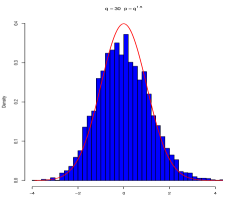
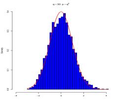
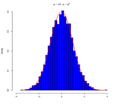
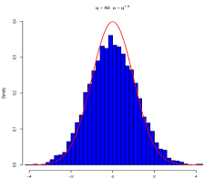
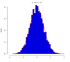
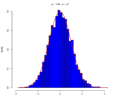
Figure 2. The plots simulate the density of $\frac{1}{2pq}\sum_{1\leq i\neq j\leq q}\big{[}(\mathbb{g}_{i}^{\prime}\mathbb{g}_{j})^{2}-p\big{]}$ in Lemma  2.10 for $(p,q)=(165,30),(900,30),(1600,40)$ in the top row, and $(p,q)=(355,50),(2500,50),(10000,100)$ in the bottom row, respectively. They match the density curve of $N(0,1)$ better as both $p$ and $q$ are larger.

Now we prove the second main result in this section.

Proof of Lemma 2.10. Since $\frac{q}{p}\to 0$, we assume that, without loss of generality, $q<p$ for all $n\geq 3$. Let

$$T_{n}=\frac{1}{pq}\sum_{1\leq i\neq j\leq q}\big{[}(\mathbb{g}_{i}^{\prime}\mathbb{g}_{j})^{2}-p\big{]},$$

which can be rewritten by

$$T_{n}=\frac{2}{pq}\sum_{j=2}^{q}\sum_{i=1}^{j-1}\big{[}(\mathbb{g}_{i}^{\prime}\mathbb{g}_{j})^{2}-p\big{]}.$$

Define $C_{0}=0$ and

$$C_{j}=\sum_{i=1}^{j-1}\big{[}(\mathbb{g}_{i}^{\prime}\mathbb{g}_{j})^{2}-p\big{]}$$

for $2\leq j\leq q$. It is easy to see

$$B_{j}:=\mathbb{E}[C_{j}|\mathcal{F}_{j-1}]=\sum_{i=1}^{j-1}\mathbb{E}[\big{(}(\mathbb{g}_{i}^{\prime}\mathbb{g}_{j})^{2}-p\big{)}|\mathcal{F}_{j-1}]=\sum_{i=1}^{j-1}(\|\mathbb{g}_{i}\|^{2}-p)$$ (4.8)

where the sigma algebra $\mathcal{F}_{k}=\sigma\big{(}\mathbb{g}_{1},\mathbb{g}_{2},\cdots,\mathbb{g}_{k}\big{)}$ for all $1\leq k\leq q.$ Thus

$$X_{j}:=C_{j}-\mathbb{E}[C_{j}|\mathcal{F}_{j-1}]=\sum_{i=1}^{j-1}\big{[}(\mathbb{g}_{i}^{\prime}\mathbb{g}_{j})^{2}-\|\mathbb{g}_{i}\|^{2}\big{]},\quad 2\leq j\leq q,$$ (4.9)

form a martingale difference with respect to the $\sigma$-algebra $(\mathcal{F}_{j})_{2\leq j\leq q}.$ Therefore $T_{n}$ can be further written by

$$T_{n}=\frac{2}{pq}\sum_{j=2}^{q}X_{j}+\frac{2}{pq}\sum_{j=2}^{q}B_{j}.$$ (4.10)

By using (4.8) and changing sums, one gets

$$\frac{2}{pq}\sum_{j=2}^{q}B_{j}=\frac{2}{pq}\sum_{i=1}^{q-1}(\|\mathbb{g}_{i}\|^{2}-p)(q-i).$$

Since $\|\mathbb{g}_{i}\|^{2}\sim\chi^{2}(p)$ for each $1\leq i\leq q$, we know ${\rm Var}(\|\mathbb{g}_{i}\|^{2}-p)={\rm Var}(\|\mathbb{g}_{i}\|^{2})=2p$. Hence,

$${\rm Var}\Big{(}\frac{1}{pq}\sum_{j=2}^{q}B_{j}\Big{)} = \frac{1}{p^{2}q^{2}}\sum_{i=1}^{q-1}(q-i)^{2}{\rm Var}(\|\mathbb{g}_{i}\|^{2}-p)$$

$$\leq \frac{2p}{p^{2}q^{2}}\cdot q^{3}=\frac{2q}{p}\to 0.$$

This together with the fact $\mathbb{E}\sum_{j=2}^{q}B_{j}=0$ indicates that

$$\frac{1}{pq}\sum_{j=2}^{q}B_{j}\stackrel{{\scriptstyle p}}{{\to}}0.$$

By (4.10), to prove the theorem, it suffices to prove

$$\frac{1}{pq}\sum_{j=2}^{q}X_{j}\to N(0,1)$$

weakly as $n\to\infty.$ By the Lindeberg-Feller central limit theorem for martingale differences (see, for example, p. 414 from [13]), it is enough to verify that

$$W_{n}:=\frac{1}{p^{2}q^{2}}\sum_{j=2}^{q}\mathbb{E}[X_{j}^{2}|\mathcal{F}_{j-1}]\stackrel{{\scriptstyle p}}{{\to}}1$$ (4.11)

and

$$\frac{1}{p^{4}q^{4}}\sum_{j=2}^{q}\mathbb{E}\big{(}X_{j}^{4}\big{)}\to 0$$ (4.12)

as $n\to\infty.$ To prove (4.11), it suffices to show

$$\mathbb{E}(W_{n})\rightarrow 1$$ (4.13)

and

$${\rm Var}(W_{n})\rightarrow 0$$ (4.14)

as $n\to\infty.$ In the rest of the proof, due to their lengths we will show the above three assertions in the order of (4.13), (4.12) and (4.14), respectively. The proof will be finished then.

The proof of (4.13). For simplicity, given $2\leq j\leq q,$ define

$$\mathbb{w}_{i}:=(\mathbb{g}_{i}^{\prime}\mathbb{g}_{j})^{2}-\|\mathbb{g}_{i}\|^{2}$$

for any $i=1,\cdots,j-1.$ Recall that $\mathbb{a}_{i}:=\frac{\mathbb{g}_{i}}{\|\mathbb{g}_{i}\|}$ and $\|\mathbb{g}_{i}\|$ are independent, we have a useful fact that

$$\mathbb{w}_{i}=\|\mathbb{g}_{i}\|^{2}[(\mathbb{a}_{i}^{\prime}\mathbb{g}_{j})^{2}-1]=\|\mathbb{g}_{i}\|^{2}(\chi-1)$$ (4.15)

given $\mathbb{g}_{i}$, where $\chi$ is a random variable with distribution $\chi^{2}(1)$ and is independent of $\|\mathbb{g}_{i}\|$. It is easy to see $X_{j}=\sum_{i=1}^{j-1}\mathbb{w}_{i}$ from (4.9). By Lemma 4.2, for any $2\leq j\leq q,$ we see

$$\mathbb{E}\big{(}X^{2}_{j}\big{)} = \sum_{i=1}^{j-1}\mathbb{E}(\mathbb{w}_{i}^{2})+\sum_{1\leq i\neq k\leq j-1}\mathbb{E}(\mathbb{w}_{i}\mathbb{w}_{k})$$

$$= \sum_{i=1}^{j-1}\mathbb{E}\big{[}\mathbb{E}(\mathbb{w}_{i}^{2}|\mathbb{g}_{i})\big{]}+\sum_{1\leq i\neq k<j}\mathbb{E}\big{(}\mathbb{E}[\mathbb{w}_{i}\mathbb{w}_{k}|\mathbb{g}_{j}]\big{)}$$

$$= 2\sum_{1\leq i<j}\mathbb{E}\|\mathbb{g}_{i}\|^{4}+\sum_{1\leq i\neq k<j}\mathbb{E}(\|\mathbb{g}_{j}\|^{2}-p)^{2}$$

$$= 2(p^{2}+2p)(j-1)+2p(j-1)(j-2),$$

where in the third equality we use the fact that $\mathbb{w}_{i}$ and $\mathbb{w}_{k}$ are conditionally independent given $\mathbb{g}_{j}$ for any $j\neq k$ and $\mathbb{E}[\mathbb{w}_{i}|\mathbb{g}_{j}]=\|\mathbb{g}_{j}\|^{2}-p.$ Thereby,

$$\mathbb{E}(W_{n})=\frac{1}{p^{2}q^{2}}\sum_{j=2}^{q}\mathbb{E}(X_{j}^{2})=\frac{(p^{2}+2p)q(q-1)+O(pq^{3})}{p^{2}q^{2}}\to 1$$

as $n\to\infty$. This justifies (4.13). In particular,

$$\sum_{j=2}^{q}\mathbb{E}(X_{j}^{2})\leq Cp^{2}q^{2}$$ (4.16)

for all $n\geq 4$, which will be used later.

The proof of (4.12). Fix $j$ with $2\leq j\leq q$. Observe that $(\mathbb{w}_{i})_{1\leq i\leq j-1}$ form again a martingale difference with respect to the sigma algebra $(\mathcal{F}_{i})_{1\leq i\leq j-1}.$ The Burkholder inequality (see, for example, [32]) says that, for any $s>1,$

$$\mathbb{E}\Big{(}\sum_{i=1}^{j-1}\mathbb{w}_{i}\Big{)}^{s}\leq C\cdot\mathbb{E}\Big{(}\sum_{i=1}^{j-1}\mathbb{w}_{i}^{2}\Big{)}^{s/2},$$

where $C$ is a universal constant depending on $s$ only. By taking $s=4$, we see from $X_{j}=\sum_{i=1}^{j-1}\mathbb{w}_{i}$ that

$$\mathbb{E}(X^{4}_{j}) \leq C\sum_{i=1}^{j-1}\mathbb{E}(\mathbb{w}_{i}^{4})+C\sum_{1\leq i\neq k\leq j-1}\mathbb{E}(\mathbb{w}_{i}^{2}\mathbb{w}_{l}^{2})$$ (4.17)

$$= C\sum_{i=1}^{j-1}\mathbb{E}[\mathbb{E}(\mathbb{w}_{i}^{4}|\mathbb{g}_{i})]+C\sum_{1\leq i\neq k\leq j-1}\mathbb{E}\big{[}\mathbb{E}(\mathbb{w}_{i}^{2}|\mathbb{g}_{j})\cdot\mathbb{E}(\mathbb{w}_{k}^{2}|\mathbb{g}_{j})\big{]}$$

by using the conditional independence. From (4.15),

$$\mathbb{E}\big{[}\mathbb{E}(\mathbb{w}_{i}^{4}|\mathbb{g}_{i})\big{]} \leq \mathbb{E}(\|\mathbb{g}_{i}\|^{8})\cdot\mathbb{E}\big{[}(\chi-1)^{4}\big{]}$$

$$= \mathbb{E}\big{(}\chi^{2}(p)^{4})\cdot\mathbb{E}\big{[}(\chi-1)^{4}\big{]}$$

$$\leq Cp^{4}$$

by Lemma 2.8. Now, from (4.6), the second sum in (4.17) is bounded by

$$\mathbb{E}\big{[}3\|\mathbb{g}_{j}\|^{4}+(p^{2}+2p)-2(p+2)\|\mathbb{g}_{j}\|^{2}\big{]}^{2}$$

$$\leq 3\big{[}\mathbb{E}(\chi^{2}(p)^{4})+(p^{2}+2p)^{2}+4(p+2)^{2}\mathbb{E}(\chi^{2}(p)^{2})\big{]}$$

$$\leq Cp^{4}$$

by the Minkowski inequality and Lemma 2.8 again. The above two estimates together with (4.17) imply

$$\mathbb{E}(X^{4}_{j})\leq C\cdot\big{[}(j-1)p^{4}+(j-1)(j-2)p^{4}]$$

for $2\leq j\leq q$, where $C$ is free of $n$ and $j$. Consequently,

$$\frac{1}{p^{4}q^{4}}\sum_{j=2}^{q}\mathbb{E}\big{(}X_{j}^{4}\big{)}\leq\frac{C}{p^{4}q^{4}}\sum_{j=2}^{q}j^{2}p^{4}\leq\frac{Cp^{4}q^{3}}{p^{4}q^{4}}\to 0$$

as $n\to\infty.$ This concludes (4.12).

The proof of (4.14). We need to prove that

$$\frac{1}{p^{4}q^{4}}{\rm Var}\bigg{[}\sum_{j=2}^{q}\mathbb{E}\big{(}X_{j}^{2}|\mathcal{F}_{j-1}\big{)}\bigg{]}\to 0$$

as $n\to\infty.$ Let us first compute $\mathbb{E}[X_{j}^{2}|\mathcal{F}_{j-1}]$. Set $\alpha_{i}=\frac{\mathbb{g}_{i}}{\|\mathbb{g}_{i}\|}$ for $1\leq i\leq q.$ Then,

$$\mathbb{E}\big{(}X_{j}^{2}|\mathcal{F}_{j-1}\big{)} = \mathbb{E}\Big{[}\big{(}\sum_{i=1}^{j-1}\mathbb{w}_{i}\big{)}^{2}|\mathcal{F}_{j-1}\Big{]}$$

$$= \sum_{i=1}^{j-1}\mathbb{E}\big{(}\mathbb{w}_{i}^{2}|\mathcal{F}_{j-1}\big{)}+I(j\geq 3)\cdot\sum_{1\leq i\neq k\leq j-1}\mathbb{E}\big{(}\mathbb{w}_{i}\mathbb{w}_{k}|\mathcal{F}_{j-1}\big{)}$$

$$= \sum_{i=1}^{j-1}\|\mathbb{g}_{i}\|^{4}\cdot\mathbb{E}[(\chi-1)^{2}]+I(j\geq 3)\cdot\sum_{1\leq i\neq k\leq j-1}\|\mathbb{g}_{i}\|^{2}\|\mathbb{g}_{k}\|^{2}\cdot$$

$$\quad\quad\quad\quad\quad\quad\quad\mathbb{E}\big{[}(\alpha_{i}^{\prime}\mathbb{g}_{j})^{2}(\alpha_{k}^{\prime}\mathbb{g}_{j})^{2}-(\alpha_{i}^{\prime}\mathbb{g}_{j})^{2}-(\alpha_{k}^{\prime}\mathbb{g}_{j})^{2}+1|\mathcal{F}_{j-1}\big{]},$$

where $I(j\geq 3)$ is the indicator function of the set $\{j\geq 3\}.$ Given $\mathcal{F}_{j-1}$, evidently $\alpha_{i}^{\prime}\mathbb{g}_{j}\sim N(0,1)$ for $1\leq i\leq j-1.$ Therefore, from Lemma 4.1 we have

$$\mathbb{E}\big{(}X_{j}^{2}|\mathcal{F}_{j-1}\big{)} = 2\sum_{i=1}^{j-1}\|\mathbb{g}_{i}\|^{4}+2I(j\geq 3)\cdot\sum_{1\leq i\neq k\leq j-1}\|\mathbb{g}_{i}\|^{2}\|\mathbb{g}_{k}\|^{2}(\alpha_{i}^{\prime}\alpha_{k})^{2}$$

$$= 2\sum_{i=1}^{j-1}\|\mathbb{g}_{i}\|^{4}+2I(j\geq 3)\cdot\sum_{1\leq i\neq k\leq j-1}(\mathbb{g}_{i}^{\prime}\mathbb{g}_{k})^{2}.$$

By changing the order of sums, it is not difficult to verify that

$$\sum_{j=2}^{q}\mathbb{E}\big{(}X_{j}^{2}|\mathcal{F}_{j-1}\big{)}=2\sum_{i=1}^{q-1}\|\mathbb{g}_{i}\|^{4}(q-i)+4\sum_{i=1}^{q-2}\sum_{k=i+1}^{q-1}(\mathbb{g}_{i}^{\prime}\mathbb{g}_{k})^{2}(q-k).$$

Therefore,

$${\rm Var}\Big{[}\sum_{j=2}^{q}\mathbb{E}\big{(}X_{j}^{2}|\mathcal{F}_{j-1}\big{)}\Big{]}$$ (4.18)

$$\leq 8\cdot{\rm Var}\Big{[}\sum_{i=1}^{q-1}\|\mathbb{g}_{i}\|^{4}(q-i)\Big{]}+32\cdot{\rm Var}\bigg{[}\sum_{i=1}^{q-2}\sum_{j=i+1}^{q-1}(\mathbb{g}_{i}^{\prime}\mathbb{g}_{j})^{2}(q-j)\bigg{]}$$

$$= 8\cdot\sum_{i=1}^{q-1}(q-i)^{2}{\rm Var}(\|\mathbb{g}_{i}\|^{4})+32\cdot{\rm Var}\bigg{[}\sum_{j=2}^{q-1}(q-j)\sum_{i=1}^{j-1}(\mathbb{g}_{i}^{\prime}\mathbb{g}_{j})^{2}\bigg{]}.$$

On the one hand, by Lemma 2.8 we know

$$\sum_{i=1}^{q-1}(q-i)^{2}{\rm Var}(\|\mathbb{g}_{i}\|^{4})\leq q^{3}\cdot{\rm Var}\big{[}\chi^{2}(p)^{2}\big{]}=8pq^{3}(p+2)(p+3).$$ (4.19)

Moreover, for $2\leq j\leq q$ fixed, recall the notation

$$\mathbb{w}_{i}:=(\mathbb{g}_{i}^{\prime}\mathbb{g}_{j})^{2}-\|\mathbb{g}_{i}\|^{2},\quad X_{j}=\sum_{i=1}^{j-1}\mathbb{w}_{i}.$$

Then

$$\sum_{i=1}^{j-1}(\mathbb{g}_{i}^{\prime}\mathbb{g}_{j})^{2}=\sum_{i=1}^{j-1}\big{(}\mathbb{w}_{i}+\|\mathbb{g}_{i}\|^{2}\big{)}=X_{j}+\sum_{i=1}^{j-1}\|\mathbb{g}_{i}\|^{2},$$

which implies

$$\sum_{j=2}^{q-1}(q-j)\sum_{i=1}^{j-1}(\mathbb{g}_{i}^{\prime}\mathbb{g}_{j})^{2} = \sum_{j=2}^{q-1}(q-j)X_{j}+\sum_{j=2}^{q-1}(q-j)\sum_{i=1}^{j-1}\|\mathbb{g}_{i}\|^{2}$$

$$= \sum_{j=2}^{q-1}(q-j)X_{j}+\sum_{i=1}^{q-2}\|\mathbb{g}_{i}\|^{2}\sum_{j=i+1}^{q-1}(q-j)$$

$$= \sum_{j=2}^{q-1}(q-j)X_{j}+\frac{1}{2}\sum_{i=1}^{q-2}\|\mathbb{g}_{i}\|^{2}(q-i-1)(q-i).$$

Consequently we have

$${\rm Var}\bigg{[}\sum_{j=2}^{q-1}(q-j)\sum_{i=1}^{j-1}(\mathbb{g}_{i}^{\prime}\mathbb{g}_{j})^{2}\bigg{]}$$ (4.20)

$$\leq 2\cdot{\rm Var}\bigg{[}\sum_{j=2}^{q-1}(q-j)X_{j}\bigg{]}+\frac{1}{2}\cdot{\rm Var}\bigg{[}\sum_{i=1}^{q-2}\|\mathbb{g}_{i}\|^{2}(q-i-1)(q-i)\bigg{]}$$

$$= 2\sum_{j=2}^{q-1}(q-j)^{2}{\rm Var}(X_{j})+\frac{1}{2}\sum_{i=1}^{q-2}(q-i-1)^{2}(q-i)^{2}{\rm Var}\big{(}\|\mathbb{g}_{1}\|^{2}\big{)}$$

$$\leq 2q^{2}\sum_{j=2}^{q}\mathbb{E}(X_{j}^{2})+q^{5}\,{\rm Var}\big{(}\|\mathbb{g}_{1}\|^{2}\big{)}$$ (4.21)

$$= C\big{(}p^{2}q^{4}+pq^{5}),$$ (4.22)

where we use the fact $(X_{j})_{2\leq j\leq q}$ is a martingale with respect to $(\mathcal{F}_{j})_{2\leq j\leq q}$ in (4.20); the trivial bounds $(q-j)^{2}\leq q^{2}$ and $(q-i-1)^{2}(q-i)^{2}\leq q^{4}$ are applied in (4.21); the last step is obtained by (4.16) and the identity ${\rm Var}\big{(}\|\mathbb{g}_{1}\|^{2}\big{)}=2p.$

Plugging (4.19) and (4.22) into (4.18), we have from the fact $q\leq p$ that

$$\frac{1}{p^{4}q^{4}}{\rm Var}\bigg{(}\sum_{j=2}^{q}\mathbb{E}[X_{j}^{2}|\mathcal{F}_{j-1}]\bigg{)}\leq\frac{Cp^{3}q^{3}}{p^{4}q^{4}}=\frac{C}{pq}\to 0$$

as $n\to\infty$. This finishes the verification of (4.14). The proof is completed. $\blacksquare$

Now we prove Lemma 2.11.

Proof of Lemma 2.11. Write ${\bf X}=({\bf g}_{1},{\bf g}_{2},\cdots,{\bf g}_{q})$ where ${\bf g}_{i}\sim N_{p}(0,{\bf I}_{p}).$ A repeatedly used fact is that $\|{\bf g}_{i}\|^{2}\sim\chi^{2}(p)$ for each $i$. Using this fact, independence, Lemma 2.8 and (4.15), we have

$$\mathbb{E}({\bf g}_{1}^{\prime}{\bf g}_{2})^{2}=p,\quad\mathbb{E}({\bf g}_{1}^{\prime}{\bf g}_{2})^{4}=3\mathbb{E}(\|{\bf g}_{1}\|^{4})=3p(p+2);$$

$$\mathbb{E}[\|{\bf g}_{1}\|^{2}\cdot({\bf g}^{\prime}_{1}{\bf g}_{2})^{2}]=p(p+2);$$

$$\mathbb{E}\big{[}({\bf g}_{1}^{\prime}{\bf g}_{2})^{2}({\bf g}_{1}^{\prime}{\bf g}_{3})^{2}\big{]}=\mathbb{E}(\|{\bf g}_{1}\|^{4})=p(p+2);$$

$$\mathbb{E}\big{[}\|{\bf g}_{1}\|^{4}({\bf g}_{1}^{\prime}{\bf g}_{2})^{2}\big{]}=\mathbb{E}(\|{\bf g}_{1}\|^{6})=p(p+2)(p+4).$$

Easily, ${\rm tr}({\bf X}^{\prime}{\bf X})=\sum_{i=1}^{q}\|{\bf g}_{i}\|^{2}$ and

$${\rm tr}[({\bf X^{\prime}X})^{2}]=\sum_{1\leq i\neq j\leq q}({\bf g}_{i}^{\prime}{\bf g}_{j})^{2}+\sum_{k=1}^{q}\|{\bf g}_{k}\|^{4}.$$ (4.23)

(i) By using the set of formulas right before (4.23), we obtain

$$\mathbb{E}{\rm tr}[({\bf X^{\prime}X})^{2}]=q(q-1)p+qp(p+2)=pq(p+q+1).$$ (4.24)

From (4.23) we see

$${\rm tr}^{2}[({\bf X^{\prime}X})^{2}]=\big{(}\sum_{k=1}^{q}\|{\bf g}_{k}\|^{4}\big{)}^{2}+\big{[}\sum_{1\leq i\neq j\leq q}({\bf g}_{i}^{\prime}{\bf g}_{j})^{2}\big{]}^{2}+2\sum_{k=1}^{q}\|{\bf g}_{k}\|^{4}\sum_{1\leq i\neq j\leq q}({\bf g}_{i}^{\prime}{\bf g}_{j})^{2}.$$ (4.25)

It is easy to check

$$\Big{(}\sum_{k=1}^{q}\|{\bf g}_{k}\|^{4}\Big{)}^{2}=\sum_{k=1}^{q}\|{\bf g}_{k}\|^{8}+\sum_{1\leq i\neq j\leq q}\|{\bf g}_{i}\|^{4}\|{\bf g}_{j}\|^{4}$$ (4.26)

and

$$\Big{[}\sum_{1\leq i\neq j\leq q}({\bf g}_{i}^{\prime}{\bf g}_{j})^{2}\Big{]}^{2} = \sum_{1\leq i\neq j\neq k\neq l\leq q}({\bf g}_{i}^{\prime}{\bf g}_{j})^{2}({\bf g}_{k}^{\prime}{\bf g}_{l})^{2}+2\sum_{1\leq i\neq j\leq q}({\bf g}_{i}^{\prime}{\bf g}_{j})^{4}$$ (4.27)

$$+4\sum_{1\leq i\neq j\neq k\leq q}({\bf g}_{i}^{\prime}{\bf g}_{j})^{2}({\bf g}_{i}^{\prime}{\bf g}_{k})^{2}$$

and

$$2\sum_{k=1}^{q}\|{\bf g}_{k}\|^{4}\sum_{1\leq i\neq j\leq q}({\bf g}_{i}^{\prime}{\bf g}_{j})^{2}=2\sum_{1\leq i\neq j\neq k\leq q}\|{\bf g}_{k}\|^{4}({\bf g}_{i}^{\prime}{\bf g}_{j})^{2}+4\sum_{1\leq i\neq j\leq q}\|{\bf g}_{i}\|^{4}({\bf g}_{i}^{\prime}{\bf g}_{j})^{2}.$$ (4.28)

By the formulas right before (4.23), Lemma 2.8, (4.26), (4.27) and (4.28), respectively, we have that

$$\mathbb{E}\Big{(}\sum_{k=1}^{q}\|{\bf g}_{k}\|^{4}\Big{)}^{2}=qp(p+2)(p+4)(p+6)+q(q-1)p^{2}(p+2)^{2}$$

and

$$\mathbb{E}\Big{[}\sum_{1\leq i\neq j\leq q}({\bf g}_{i}^{\prime}{\bf g}_{j})^{2}\Big{]}^{2} = q(q-1)(q-2)(q-3)p^{2}+6p(p+2)q(q-1)$$

$$+4p(p+2)q(q-1)(q-2)$$

and

$$2\mathbb{E}\Big{[}\sum_{k=1}^{q}\|{\bf g}_{k}\|^{4}\sum_{1\leq i\neq j\leq q}({\bf g}_{i}^{\prime}{\bf g}_{j})^{2}\Big{]} = 2q(q-1)(q-2)p^{2}(p+2)$$

$$+4q(q-1)p(p+2)(p+4).$$

Putting all these three expressions back into (4.25), one gets

$$\mathbb{E}{\rm tr}^{2}[({\bf X^{\prime}X})^{2}] = qp(p+2)(p+4)(p+6)+q(q-1)p^{2}(p+2)^{2}$$

$$+q(q-1)(q-2)(q-3)p^{2}+6p(p+2)q(q-1)$$

$$+4p(p+2)q(q-1)(q-2)$$

$$+2q(q-1)(q-2)p^{2}(p+2)+4q(q-1)p(p+2)(p+4).$$

This together with (4.24) implies

$${\rm Var}\big{(}{\rm tr}[({\bf X^{\prime}X})^{2}]\big{)}=4p^{2}q^{2}+8pq(p+q)^{2}+20pq(p+q+1).$$

(ii) Recall (4.23). By independence,

$${\rm Cov}\big{(}{\rm tr}({\bf X}^{\prime}{\bf X}),{\rm tr}[({\bf X}^{\prime}{\bf X})^{2}]\big{)} = {\rm Cov}\Big{(}\sum_{i=1}^{q}\|{\bf g}_{i}\|^{2},\sum_{i=1}^{q}\|{\bf g}_{i}\|^{4}+\sum_{1\leq i\neq j\leq q}({\bf g}^{\prime}_{i}{\bf g}_{j})^{2}\Big{)}$$

$$= \sum_{i=1}^{q}{\rm Cov}\big{(}\|{\bf g}_{i}\|^{2},\|{\bf g}_{i}\|^{4}\big{)}+2\sum_{1\leq i\neq j\leq q}{\rm Cov}(\|{\bf g}_{i}\|^{2},({\bf g}^{\prime}_{i}{\bf g}_{j})^{2})$$

$$= \sum_{i=1}^{q}\big{[}\mathbb{E}(\|{\bf g}_{i}\|^{6})-\mathbb{E}(\|{\bf g}_{i}\|^{4})\cdot\mathbb{E}(\|{\bf g}_{i}\|^{2})\big{]}$$

$$+2\sum_{1\leq i\neq j\leq q}\big{(}\mathbb{E}[\|{\bf g}_{i}\|^{2}\cdot({\bf g}^{\prime}_{i}{\bf g}_{j})^{2}]-\mathbb{E}(\|{\bf g}_{i}\|^{2})\cdot\mathbb{E}({\bf g}^{\prime}_{i}{\bf g}_{j})^{2}\big{)}.$$

From the formulas right before (4.23) again, we have

$${\rm Cov}\big{(}{\rm tr}[{\bf X}^{\prime}{\bf X}],{\rm tr}[({\bf X}^{\prime}{\bf X})^{2}]\big{)} =\sum_{i=1}^{q}[p(p+2)(p+4)-p^{2}(p+2)]+2\sum_{1\leq i\neq j\leq q}[p(p+2)-p^{2}]$$

$$=4pq(p+2)+4pq(q-1)$$

$$=4pq(p+q+1).$$

The proof is completed now. $\blacksquare$

5. This part is for referees only

Proof of Lemma 3.5. Suppose the conclusion is not true, that is, $\liminf_{n\to\infty}f_{n}(p_{n},q_{n})=0$ for some sequence $\{(p_{n},q_{n})\}_{n=1}^{\infty}$ with $1\leq p_{n},q_{n}\leq n$ for each $n\geq 1$ and $\lim_{n\to\infty}(p_{n}q_{n}^{2})/n=\alpha\in(0,\infty)$. Then there exists a subsequence $\{n_{k};\,k\geq 1\}$ satisfying $1\leq p_{n_{k}},q_{n_{k}}\leq n_{k}$ for all $k\geq 1$ and $\lim_{k\to\infty}(p_{n_{k}}q_{n_{k}}^{2})/n_{k}=\alpha\in(0,\infty)$ such that

$$\lim_{k\to\infty}f_{n_{k}}(p_{n_{k}},q_{n_{k}})=0.$$ (5.1)

There are two possibilities: $\liminf_{k\to\infty}q_{n_{k}}<\infty$ and $\liminf_{k\to\infty}q_{n_{k}}=\infty$. Let us discuss the two cases separately.

(a). Assume $\liminf_{k\to\infty}q_{n_{k}}<\infty$. Then there exists a further subsequence $\{n_{k_{j}}\}_{j=1}^{\infty}$ such that $q_{n_{k_{j}}}\equiv m\geq 1$. For convenience of notation, write $\bar{n}_{j}=n_{k_{j}}$ for all $j\geq 1.$ The condition $\lim_{n\to\infty}\frac{p_{n}q_{n}^{2}}{n}=\alpha$ implies that $\lim_{j\to\infty}\frac{p_{\bar{n}_{j}}}{\bar{n}_{j}}=\frac{\alpha}{m^{2}}\in(0,1].$ By (5.1) and the monotonocity,

$$\lim_{j\to\infty}f_{\bar{n}_{j}}(p_{\bar{n}_{j}},1)=\lim_{j\to\infty}f_{\bar{n}_{j}}(p_{\bar{n}_{j}},q_{\bar{n}_{j}})=0.$$ (5.2)

Define $\tilde{p}_{\bar{n}_{j}}=[p_{\bar{n}_{j}}/2]+1$ for all $j\geq 1.$ Then, $\lim_{j\to\infty}\frac{\tilde{p}_{\bar{n}_{j}}}{\bar{n}_{j}}=c:=\frac{\alpha}{2m^{2}}\in(0,\frac{1}{2}].$ Construct a new sequence such that

$$\tilde{p}_{r}=\begin{cases}\tilde{p}_{\bar{n}_{j}},&\text{if $r=\bar{n}_{j}$ for some $j\geq 1$};\\ [cr]\vee 1,&\text{if not}\end{cases}$$

and $\tilde{q}_{r}=1$ for $r=1,2,\cdots.$ Obviously, $\tilde{p}_{\bar{n}_{j}}\leq p_{\bar{n}_{j}}$ for each $j\geq 1.$ It is easy to check $1\leq\tilde{p}_{r},\tilde{q}_{r}\leq r$ for all $r\geq 1$ and $\lim_{r\to\infty}\tilde{p}_{r}/r=c\in(0,1/2)$. So $\{(\tilde{p}_{r},\tilde{q}_{r});\,r\geq 1\}$ satisfies condition (i), and hence $\liminf_{r\to\infty}f_{r}(\tilde{p}_{r},\tilde{q}_{r})>0$ by (3.15). This contradicts (5.2) since $f_{r}(\tilde{p}_{r},\tilde{q}_{r})=f_{\bar{n}_{j}}(\tilde{p}_{\bar{n}_{j}},1)\leq f_{\bar{n}_{j}}(p_{\bar{n}_{j}},1)$ if $r=\bar{n}_{j}$ for some $j\geq 1$ by monotonocity.

(b). Assume $\liminf_{k\to\infty}q_{n_{k}}=\infty$. Then $\lim_{k\to\infty}q_{n_{k}}=\infty$. Define

$$\tilde{p}_{r}=\begin{cases}p_{n_{k}},&\text{if $r=n_{k}$ for some $k\geq 1$};\\ [r^{1/3}],&\text{if not}\end{cases}$$

and

$$\tilde{q}_{r}=\begin{cases}q_{n_{k}},&\text{if $r=n_{k}$ for some $k\geq 1$};\\ \big{(}[\sqrt{\alpha}r^{1/3}]+1\big{)}\wedge r,&\text{if not}.\end{cases}$$

Trivially, $1\leq\tilde{p}_{r},\tilde{q}_{r}\leq r$ for all $r\geq 1$, $\lim_{r\to\infty}\tilde{q}_{r}=\infty$ and $\lim_{r\to\infty}\tilde{p}_{r}\tilde{q}_{r}^{2}/r=\alpha$. By (ii),

$$\liminf_{k\to\infty}f_{n_{k}}(p_{n_{k}},q_{n_{k}})\geq\liminf_{r\to\infty}f_{r}(\tilde{p}_{r},\tilde{q}_{r})>0$$

since $\tilde{p}_{r}=p_{n_{k}}$ and $\tilde{q}_{r}=q_{n_{k}}$ if $r=n_{k}$. This contradicts (5.1).

In summary, each of the cases that $\liminf_{k\to\infty}q_{n_{k}}<\infty$ and that $\liminf_{k\to\infty}q_{n_{k}}=\infty$ results with a contradiction. Therefore, we obtain our desired conclusion. $\blacksquare$

Acknowledgement. We thank Professor Xinmei Shen for very helpful communications. In particular we thank her for producing Figure 2 for us.