Accelerated Distributed Dual Averaging over Evolving Networks of Growing Connectivity

Abstract

We consider the problem of accelerating distributed optimization in multi-agent networks by sequentially adding edges. Specifically, we extend the distributed dual averaging (DDA) subgradient algorithm to evolving networks of growing connectivity and analyze the corresponding improvement in convergence rate. It is known that the convergence rate of DDA is influenced by the algebraic connectivity of the underlying network, where better connectivity leads to faster convergence. However, the impact of network topology design on the convergence rate of DDA has not been fully understood. In this paper, we begin by designing network topologies via edge selection and scheduling in an offline manner. For edge selection, we determine the best set of candidate edges that achieves the optimal tradeoff between the growth of network connectivity and the usage of network resources. The dynamics of network evolution is then incurred by edge scheduling. Furthermore, we provide a tractable approach to analyze the improvement in the convergence rate of DDA induced by the growth of network connectivity. Our analysis reveals the connection between network topology design and the convergence rate of DDA, and provides quantitative evaluation of DDA acceleration for distributed optimization that is absent in the existing analysis. Lastly, numerical experiments show that DDA can be significantly accelerated using a sequence of well-designed networks, and our theoretical predictions are well matched to its empirical convergence behavior.

I Introduction

Optimization over networks has found a wide range of applications in parallel computing [1, 2], sensor networks [3, 4], communication systems [5, 6], machine learning [7] and power grids [8]. Many such problems fall under the framework of distributed optimization in order to minimize the network loss function, given as a sum of local objective functions accessed by agents, e.g., cores in massive parallel computing. The ultimate goal is to achieve the solution of the network-structured optimization problem by using only local information and in-network communications.

In this paper, we investigate the impact of network topology design on the convergence rate of distributed optimization algorithms. To be specific, we focus on the convergence analysis of the distributed dual averaging (DDA) subgradient algorithm [9] under well-designed time-evolving networks, where edges are sequentially added. There are several motivations for DDA. First, DDA provides a general distributed optimization framework that can handle problems involving nonsmooth objective functions and constraints. In contrast, some recently developed accelerated distributed algorithms [10, 11, 12, 13, 14] are limited to problems satisfying conditions such as strong convexity, smoothness, and smooth+nonsmooth composite objectives. Second, it was shown by Nesterov [15] that the use of dual averaging guarantees boundedness of the sequence of primal solution points even in the case of an unbounded feasible set. This is in contrast with some recent algorithms [16, 17], which require boundedness of the feasible set for the convergence analysis. Third, the convergence rate of DDA [9] can be decomposed into two additive terms: one reflecting the suboptimality of first-order algorithms and the other representing the network effect. The latter has a tight dependence on the algebraic connectivity [18] of the network topology. This enables us to accelerate DDA by making the network fast mixing with increasing network connectivity. However, the use of desired time-evolving networks introduces new challenges in distributed optimization: a) How to sequentially add edges to a network to maximize DDA acceleration? b) How to evaluate the improvement in the convergence rate of DDA induced by the growth of network connectivity? c) How to connect the dots between the strategy of topology design and the convergence behavior of DDA? In this paper, we aim to answer these questions in the affirmative.

I-A Prior and related work

There has been a significant amount of research on developing distributed computation and optimization algorithms in multi-agent networked systems [19, 20, 21, 22, 23, 24, 25, 26, 27, 28, 29, 10, 11, 12, 13, 14, 30, 31, 32, 33]. Early research efforts focus on the design of consensus algorithms for distributed averaging, estimation and filtering, where ‘consensus’ means to reach agreement on a common decision for a group of agents [19, 20, 21, 22, 23, 24]. In [25], a strict consensus protocol was relaxed to a protocol that only ensures neighborhood similarity between agents’ decisions. Although the existing distributed algorithms are essentially different, they share a similar consensus-like step for information averaging, whose speed is associated with the spectral properties of the underlying networks.

In addition to distributed averaging, estimation and filtering, many distributed algorithms have been developed to solve general optimization problems [26, 27, 28, 29, 10, 11, 12, 13, 14, 30, 31, 32, 33]. In [26, 27, 28, 29], distributed subgradient algorithms involving the consensus step were studied under various scenarios, e.g., networks with communication delays, dynamic topologies, link failures, and push-sum averaging protocols. In [10] and [11], fast distributed gradient methods were proposed under both deterministically and randomly time-varying networks. It was shown that a faster convergence rate can be achieved by applying Nesterov’s acceleration step [34] when the objective function is smooth. In [12] and [13], accelerated first-order algorithms were proposed, which utilize the historical information and harness the function smoothness to obtain a better estimation of the gradient. In [14], a distributed proximal gradient algorithm was developed for smooth+nonsmooth composite optimization. However, the complexity of this algorithm is determined by the complexity of implementing the proximal operation, which could be computationally expensive for some forms of the nonsmooth term in the objective function. In [30], under the assumption of a static network, a probabilistic node selection scheme was proposed to accelerate the distributed subgradient algorithm in terms of reducing the overall per-node communication and gradient computation cost. Different from [10, 11, 12, 13, 14, 30], we consider a more general problem setting that allows both the objective functions and constraints to be non-smooth. In addition, we perform distributed optimization over a dynamic changing network topology, and we consider the resource limited scenario where good network topology design is used to optimize performance (minimize error) subject to constraints on the number of communication links in the network. We reveal how the edge addition scheme affects the network mixing time and the error of a distributed optimization algorithm. In addition to the first-order algorithms, distributed implementations of Newton method and an operator splitting method, alternating direction method of multipliers (ADMM), were developed in [31, 32, 33]. Compared to the first-order algorithms, second-order methods and ADMM have faster convergence rate but at the cost of higher computational complexity.

DDA [9] has attracted recent attention in signal processing, distributed control, and online learning [35, 36, 37, 38, 39]. In [35], it was shown that DDA is robust to communication delays, and the resulting error decays at a sublinear rate. In [36], a push-sum consensus step was combined with DDA that leads to several appealing convergence properties, e.g., the sublinear convergence rate without the need of a doubly stochastic protocol. In [37], DDA was studied when the communications among agents are either deterministically or probabilistically quantized. In [38, 39], online versions of DDA were developed when uncertainties exist in the environment so that the cost function is unknown to local agents prior to decision making. Reference [38] utilized coordinate updating protocols in DDA when the global objective function is inseparable. In [39], a distributed weighted dual averaging algorithm was proposed for online learning under switching networks.

I-B Motivation and contributions

Since the convergence rate of DDA relies on the algebraic connectivity of network topology [9], it is possible to accelerate DDA by using well-designed networks. In this paper, the desired networks are assumed to possess growing algebraic connectivity in time. The rationale behind that is elaborated on as below. First, it was empirically observed in our earlier work [40] that the growth of network connectivity could significantly improve the convergence rate of DDA compared to the case of using a static network. Therefore, distributed optimization can initially be performed over a sparse network of low computation and communication cost, and then be accelerated via a sequence of well-designed networks for improved convergence. This is particularly appealing to applications in distributed estimation/optimization with convergence time constraints. Second, the case of growing connectivity is inspired by real-world scenarios. One compelling example is in adaptive mesh parallel scientific computing where the network corresponds to grid points in the mesh and optimization is performed by solving partial differential equations over a domain that is successively and adaptively refined over the network as time progresses [41]. As another example, the accumulated connectivity of online social networks increases over time when users establish new connections (e.g., time-evolving friendship in Facebook or LinkedIn). Another example arises in the design of resilient hardened physical networks [42, 43], where adding edges or rewiring existing edges increases network connectivity and robustness to node or edge failures.

Our main contributions are twofold. First, we propose an offline optimization approach for topology design via edge selection and scheduling. The proposed approach is motivated by the fact that the algebraic connectivity is monotone increasing in the edge set [44, 45], and thus a well-connected network can be obtained via edge additions. In the stage of edge selection, we determine the best candidate edges that achieve optimal tradeoffs between the growth of network connectivity and the usage of network resources. The selected edges determined by our offline optimization method are then scheduled to update the network topology for improved convergence of DDA. Second, we provide a general convergence analysis that reveals the connection between the solution of topology design and the convergence rate of DDA. This leads to a tractable approach to analyze the improvement in the convergence rate of DDA induced by the growth of network connectivity. Extensive numerical results show that our theoretical predictions are well matched to the empirical convergence behavior of the accelerated DDA algorithm under well-designed networks.

I-C Outline

The rest of the paper is organized as follows. In Section II, we introduce the concept of distributed optimization and DDA. In Section III, we formulate two types of problems for edge selection, and provide a dynamic model to incorporate the effect of edge scheduling on DDA. In Section IV, we develop efficient optimization methods to solve the problems of edge selection. In Section V, we analyze the convergence properties of DDA under evolving networks of growing connectivity. In Section VI, we demonstrate the effectiveness of DDA over well-designed networks through numerical examples. Finally, in Section VII we summarize our work and discuss future research directions.

II Preliminaries: Graph, Distributed Optimization and Distributed Dual Averaging

In this section, we provide a background on the graph representation of a multi-agent network, the distributed optimization problem, and the distributed dual averaging algorithm.

II-A Graph representation

A graph yields a succinct representation of interactions among agents or sensors over a network. Let $\mathcal{G}_{t}=(\mathcal{V},\mathcal{E}_{t})$ denote a time-varying undirected unweighted graph at time $t=0,1,\ldots,T$, where $\mathcal{G}_{0}$ is the initial graph, $\mathcal{V}$ is a node set with cardinality $|\mathcal{V}|=n$, $\mathcal{E}_{t}\subseteq[n]\times[n]$ is an edge set with cardinality $|\mathcal{E}_{t}|=m_{t}$, and $T$ is the length of time horizon. Here for ease of notation, we denote by $[n]$ the integer set $\{1,2,\ldots,n\}$. Let $l\sim(i,j)$ denote the $l$th edge of $\mathcal{E}_{t}$ that connects nodes $i$ and $j$. Without loss of generality, the ordering of edges is given a priori. The set of neighbors of node $i$ at time $t$ is denoted by $\mathcal{N}_{i}(t)=\{j~{}|~{}(i,j)\in\mathcal{E}_{t}\}\cup\{i\}$.

A graph is commonly represented by an adjacency matrix or a graph Laplacian matrix. Let $\mathbf{A}_{t}$ be the adjacency matrix of $\mathcal{G}_{t}$, where $[\mathbf{A}_{t}]_{ij}=1$ for $(i,j)\in\mathcal{E}_{t}$ and $[\mathbf{A}_{t}]_{ij}=0$, otherwise. Here $[\mathbf{X}]_{ij}$ (or $\mathbf{X}_{ij}$) denotes the $(i,j)$-th entry of a matrix $\mathbf{X}$. The graph Laplacian matrix is defined as $\mathbf{L}_{t}=\mathbf{D}_{t}-\mathbf{A}_{t}$, where $\mathbf{D}_{t}$ is a degree diagonal matrix, whose $i$-th diagonal entry is given by $\sum_{j}[\mathbf{A}_{t}]_{ij}$. The graph Laplacian matrix is positive semidefinite, and has a zero eigenvalue $\lambda_{n}=0$ with eigenvector ${\color[rgb]{0,0,0}(1/\sqrt{n})}\mathbf{1}$. Here $\mathbf{1}$ is the column vector of ones. In this paper, eigenvalues are sorted in decreasing order of magnitude, namely, $\lambda_{i}\geq\lambda_{j}$ if $i\leq j$.

The second-smallest eigenvalue $\lambda_{n-1}(\mathbf{L}_{t})$ of $\mathbf{L}_{t}$ is known as the algebraic connectivity [18], which is positive if and only if the graph is connected, namely, there exists a path between every pair of distinct nodes. In this paper we assume that $\mathcal{G}_{t}$ is connected at each time. As will be evident later, it is beneficial to express the graph Laplacian matrix as a product of incidence matrix

$$\mathbf{L}=\mathbf{H}\mathbf{H}^{T}=\sum_{l=1}^{m}\mathbf{a}_{l}\mathbf{a}_{l}^{T},$$ (1)

where for notational simplicity, we drop the time index without loss of generality, $\mathbf{H}=[\mathbf{a}_{1},\ldots,\mathbf{a}_{m}]\in\mathbb{R}^{n\times m}$ is the incidence matrix of graph $\mathcal{G}$ with $n$ nodes and $m$ edges, and $\mathbf{a}_{l}$ is known as an edge vector corresponding to the edge $l\sim(i,j)$ with entries $[\mathbf{a}_{l}]_{i}=1$, $[\mathbf{a}_{l}]_{j}=-1$ and $0$s elsewhere.

II-B Distributed optimization

We consider a convex optimization problem, where the network cost, given by a sum of local objective functions at agents/sensors, is minimized subject to a convex constraint. That is,

$$\begin{array}[]{ll}\displaystyle\operatorname*{\text{minimize}}&\displaystyle f(\mathbf{x})\mathrel{\mathop{:}}=\frac{1}{n}\sum_{i=1}^{n}f_{i}(\mathbf{x})\\ \operatorname*{\text{subject to}}&\mathbf{x}\in\mathcal{X},\end{array}$$ (4)

where $\mathbf{x}\in\mathbb{R}^{p}$ is the optimization variable, $f_{i}$ is convex and $L$-Lipschitz continuous, and $\mathcal{X}$ is a closed (not necessarily bounded) convex set containing the origin. A concrete example of (4) is a distributed estimation problem, where $f_{i}$ is a square loss and $\mathbf{x}$ is an unknown parameter to be estimated. The graph $\mathcal{G}_{t}$ imposes communication constraints on distributed optimization to solve problem (4): Each node $i$ only accesses to the local cost function $f_{i}$ and can communicate directly only with nodes in its neighborhood $\mathcal{N}_{i}(t)$ at time $t$.

II-C Distributed dual averaging (DDA)

Throughout this paper we employ the DDA algorithm, which was first proposed in [9], to solve problem (4). In DDA, each node $i\in\mathcal{V}$ iteratively performs the following two steps

$$\mathbf{z}_{i}(t+1)=\sum_{j\in\mathcal{N}_{i}(t)}[\mathbf{P}_{t}]_{ji}\,\mathbf{z}_{j}(t)+\mathbf{g}_{i}(t)$$ (5)

$$\mathbf{x}_{i}(t+1)=\operatornamewithlimits{arg\,min}_{\mathbf{x}\in\mathcal{X}}\left\{\mathbf{z}_{i}(t+1)^{T}\mathbf{x}+\frac{1}{\alpha_{t}}\psi(\mathbf{x})\right\},$$ (6)

where $\mathbf{z}_{i}(t)\in\mathbb{R}^{d}$ is a newly introduced variable for node $i$ at time $t$, $\mathbf{P}_{t}\in\mathbb{R}^{n\times n}$ is a matrix of non-negative weights that preserves the zero structure of the graph Laplacian $\mathbf{L}_{t}$, $\mathbf{g}_{i}(t)$ is a subgradient of $f_{i}(\mathbf{x})$ at $\mathbf{x}=\mathbf{x}(t)$, $\psi(\mathbf{x})$ is a regularizer for stabilizing the update, and $\{\alpha_{t}\}_{t=0}^{\infty}$ is a non-increasing sequence of positive step-sizes.

In (6), $\psi(\mathbf{x})$ is also known as a proximal function, which is assumed to be $1$-strongly convex with respect to a generic norm $\|\cdot\|$, and $\psi(\mathbf{x})>0$ and $\psi(\mathbf{0})=0$. In particular, when $\|\cdot\|$ is the $\ell_{2}$ norm, we obtain the canonical proximal function $\psi(\mathbf{x})=(1/2)\|\mathbf{x}\|_{2}^{2}$. The weight matrix $\mathbf{P}_{t}$ in (5) is assumed to be doubly stochastic, namely, $\mathbf{1}^{T}\mathbf{P}_{t}=\mathbf{1}^{T}$ and $\mathbf{P}_{t}\mathbf{1}=\mathbf{1}$. A common choice of $\mathbf{P}_{t}$ that respects the graph structure of $\mathcal{G}_{t}$ is given by [9]

$$\mathbf{P}_{t}=\mathbf{I}-\frac{1}{2(1+\delta_{\max})}\mathbf{L}_{t},$$ (7)

where $\delta_{\max}$ is the maximum degree of $\{\mathcal{G}_{t}\}$, and $\mathbf{P}_{t}$ is positive semidefinite [46]. It is worth mentioning that if $\mathbf{L}_{t}=\mathbf{L}_{0}$ for $t\in[T]$, DDA is performed under a static network [35, 36, 9].

III Problem Formulation

In this section, we begin by introducing the concept of growing connectivity. We then formulate the problem of edge selection, which strikes a balance between network connectivity and network resources. Lastly, we link DDA with the procedure of edge scheduling.

III-A Evolving networks of growing connectivity

It is known from [47] that the algebraic connectivity provides a lower bound on the node/edge connectivity, which is the least number of node/edge removals that disconnects the graph. We refer to $\mathcal{G}_{t}$ as a dynamic network of growing connectivity if its algebraic connectivity is monotonically increasing in time, namely,

$$0<\lambda_{n-1}(\mathbf{L}_{0})\leq\lambda_{n-1}(\mathbf{L}_{1})\leq\ldots\leq\lambda_{n-1}(\mathbf{L}_{T}).$$ (8)

Based on (7), we equivalently obtain

$$\sigma_{2}(\mathbf{P}_{0})\geq\sigma_{2}(\mathbf{P}_{1})\geq\ldots\geq\sigma_{2}(\mathbf{P}_{T}),$$ (9)

where $\sigma_{2}(\mathbf{P}_{t})$ is the second-largest singular value of $\mathbf{P}_{t}$. In this paper, we aim to improve the convergence rate of DDA with the aid of designing networks of growing connectivity.

III-B Edge selection

Since the algebraic connectivity is monotone increasing in the edge set, a well-connected network can be obtained via edge additions [44]. Given an initial graph $\mathcal{G}_{0}$, it is known from (1) that the Laplacian matrix of the modified graph by adding new edges can be expressed as

$$\mathbf{L}(\mathbf{w})=\mathbf{L}_{0}+\sum_{l=1}^{K}w_{l}\mathbf{a}_{l}\mathbf{a}_{l}^{T},~{}\mathbf{w}\in\{0,1\}^{K},$$ (10)

where $K=n(n-1)/2-m_{0}$ is the maximum number of edges that can be added to $\mathcal{G}_{0}$, namely, edges in the complement of $\mathcal{G}_{0}$, $w_{l}\in\{0,1\}$ is a Boolean variable indicating whether or not the $l$th candidate edge is selected, and $\mathbf{a}_{l}\in\mathbb{R}^{n}$ is the edge vector corresponding to the added edge $l$ defined in (1).

Edge addition makes a network better-connected but consumes more network resources, e.g., bandwidth and energy for inter-node communications. Therefore, we formulate an optimization problem for edge selection, which seeks the optimal tradeoff between the network connectivity and the resource consumption due to edge addition. That is,

$$\begin{array}[]{ll}\displaystyle\operatorname*{\text{minimize}}_{\mathbf{w}\in\mathbb{R}^{K}}&n-\lambda_{n-1}\left(\mathbf{L}(\mathbf{w})\right)+\gamma\mathbf{c}^{T}\mathbf{w}\\ \operatorname*{\text{subject to}}&\mathbf{w}\in\{0,1\}^{K},\end{array}$$ (13)

where $\mathbf{L}(\mathbf{w})$ is given by (10), the term $n-\lambda_{n-1}(\mathbf{L}(\mathbf{w}))$ represents the ‘distance’ to the maximum algebraic connectivity $n$ determined by the complete graph, $\mathbf{c}=[c_{1},\ldots,c_{K}]^{T}$, $c_{l}$ is a known cost associated with the $l$th edge, e.g., communication cost proportional to the distance of two nodes, and $\gamma>0$ is a regularization parameter to characterize the relative importance of achieving a large network connectivity versus consuming a few network resources. Note that if $\mathbf{c}=\mathbf{1}$ in (13), the solution of the problem yields a tradeoff between the network connectivity and the number of selected edges.

If the number of selected edges (denoted by $k$) is given a priori, we can modify problem (13) as

$$\begin{array}[]{ll}\displaystyle\operatorname*{\text{minimize}}_{\mathbf{w}\in\mathbb{R}^{K}}&n-\lambda_{n-1}(\mathbf{L}(\mathbf{w}))+\gamma\mathbf{c}^{T}\mathbf{w}\\ \operatorname*{\text{subject to}}&\mathbf{w}\in\{0,1\}^{K},\quad\mathbf{1}^{T}\mathbf{w}=k.\end{array}$$ (16)

Different from (13), by varying the regularization parameter $\gamma$, the solution of problem (16) strikes a balance between the network connectivity and the communication cost due to edge rewiring rather than edge addition under the candidate edge set.

We remark that problems (13)-(16) can be solved offline prior to distributed optimization using edges in the set complentary to the initial graph $\mathcal{G}_{0}$, the regularization parameter $\gamma$, the edge cost $\mathbf{c}$, and/or the number of selected edges $k$. The formulation (13)-(16) specifies the best locations to add the edges, since the optimization variable $\mathbf{w}$ encodes which candidate edge is selected. In (13)-(16), the regularization parameter $\gamma$ controls the penalty on communication cost. The regularization term could be replaced with a ‘hard’ constraint on the communication cost, $\mathbf{c}^{T}\mathbf{w}\leq\eta$, where $\eta$ is the maximum cost to be consumed, and similar to $\gamma$, a tradeoff between network connectivity and communication cost can be achieved by varying $\eta$.

III-C Edge scheduling versus DDA

Given the solution of problem (13) or (16), we propose an algorithm for scheduling edge addition, generating a time-evolving network of growing connectivity. And thus, the problem of edge scheduling arises. For ease of updating network, we assume that at most one edge is added at each time step. Such an assumption is commonly used in the design of scheduling protocols for resource management [48, 49, 50]. The graph Laplacian then follows the dynamical model

$$\mathbf{L}_{t}=\mathbf{L}_{t-1}+u_{t}\mathbf{a}_{l_{t}}\mathbf{a}_{l_{t}}^{T},~{}u_{t}\in\{0,1\},~{}l_{t}\in\mathcal{E}_{\mathrm{sel}}-\mathcal{E}_{t-1}$$ (17)

where $u_{t}$ encodes whether or not a selected edge is added to $\mathbf{L}_{t-1}$, $\mathbf{a}_{l_{t}}$ is an edge vector, and $l_{t}$ is the edge index among the candidate edges $\mathcal{E}_{\mathrm{sel}}-\mathcal{E}_{t-1}$. Here $\mathcal{E}_{\mathrm{sel}}\mathrel{\mathop{:}}=\{l\sim(i,j)\,|\,w_{l}^{*}=1\}$, $\mathbf{w}^{*}$ is the solution of problem (13) or (16), $\mathcal{E}_{t-1}$ is the edge set corresponding to $\mathcal{G}_{t-1}$, and $\mathcal{E}_{\mathrm{sel}}-\mathcal{E}_{t-1}$ is the set of all elements that are members of $\mathcal{E}_{\mathrm{sel}}$ but not members of $\mathcal{E}_{t-1}$.

Based on (17), we seek the optimal scheduling scheme $\{u_{t}\}$ and $\{l_{t}\}$ such that the convergence rate of DDA is the fastest possible. Similar to solving problem (13) or (16), an offline greedy edge scheduling algorithm will be used. We summarize the DDA algorithm in conjunction with network topology design in Fig. 1.

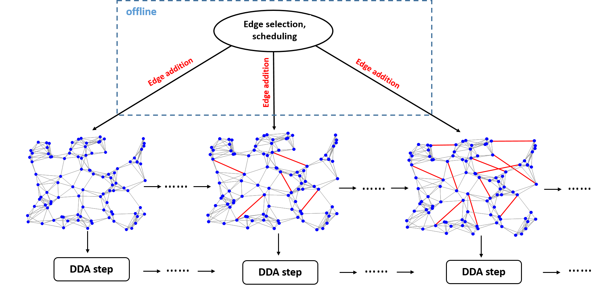
Figure 1: DDA in conjunction with topology design.

IV Optimization Methods for Topology Design

In this section, we first show that edge selection problem (13) and (16) can be solved via semidefinite programing. To improve the computational efficiency, we then present the projected subgradient algorithm and the greedy algorithm that scale more gracefully with problem size. Lastly, we discuss the decentralized edge selection method.

We begin by reformulating problems (13) and (16) as

$$\begin{array}[]{ll}\displaystyle\operatorname*{\text{minimize}}_{\mathbf{w}\in\mathbb{R}^{K}}&n\lambda_{1}\left(\mathbf{P}(\mathbf{w})-{\mathbf{1}\mathbf{1}^{T}}/{n}\right)+\gamma\mathbf{c}^{T}\mathbf{w}\\ \operatorname*{\text{subject to}}&\mathbf{w}\in\mathcal{T}_{1},~{}\text{or}~{}~{}\mathbf{w}\in\mathcal{T}_{2},\end{array}$$ (20)

where $\mathbf{P}(\mathbf{w})\mathrel{\mathop{:}}=\mathbf{I}-(1/n)\mathbf{L}(\mathbf{w})$, which is positive semidefinite since $\lambda_{1}(\mathbf{L}(\mathbf{w}))\leq n$ [51], and $\mathcal{T}_{1}$ and $\mathcal{T}_{2}$ denote constraints of problems (13) and (16), respectively. In the objective function of problem (20), we have used the fact that

$$\lambda_{n-1}(\mathbf{L}(\mathbf{w})) =n[1-\lambda_{2}(\mathbf{P}(\mathbf{w}))]$$

$$=n-n\lambda_{1}(\mathbf{P}(\mathbf{w})-{\mathbf{1}\mathbf{1}^{T}}/{n}).$$ (21)

The rationale behind introducing $\mathbf{P}(\mathbf{w})$ is that we can express the second-smallest eigenvalue $\lambda_{n-1}(\mathbf{L}(\mathbf{w}))$ in the form of the maximum eigenvalue $\lambda_{1}(\mathbf{P}(\mathbf{w})-{\mathbf{1}\mathbf{1}^{T}}/{n})$. The latter is more computationally efficient.

Moreover if the Boolean constraint $\mathbf{w}\in\{0,1\}^{K}$ is relaxed to its convex hull $\mathbf{w}\in[0,1]^{K}$, we obtain the convex program

$$\begin{array}[]{ll}\displaystyle\operatorname*{\text{minimize}}_{\mathbf{w}\in\mathbb{R}^{K}}&n\lambda_{1}\left(\mathbf{P}(\mathbf{w})-{\mathbf{1}\mathbf{1}^{T}}/{n}\right)+\gamma\mathbf{c}^{T}\mathbf{w}\\ \operatorname*{\text{subject to}}&\mathbf{w}\in\mathcal{C}_{1},~{}\text{or}~{}~{}\mathbf{w}\in\mathcal{C}_{2},\end{array}$$ (24)

where $\mathcal{C}_{1}=\{\mathbf{w}\,|\,\mathbf{w}\in[0,1]^{K}\}$, and $\mathcal{C}_{2}=\{\mathbf{w}\,|\,\mathbf{w}\in\mathcal{C}_{1},\mathbf{1}^{T}\mathbf{w}=k\}$. Problem (24) is convex since $\lambda_{1}\left(\mathbf{P}(\mathbf{w})-{\mathbf{1}\mathbf{1}^{T}}/{n}\right)$ can be described as the pointwise supremum of linear functions of $\mathbf{w}$ [52],

$$\lambda_{1}\left(\mathbf{P}(\mathbf{w})-{\mathbf{1}\mathbf{1}^{T}}/{n}\right)=\displaystyle\sup_{\|\mathbf{y}\|_{2}=1}\{\mathbf{y}^{T}\mathbf{P}(\mathbf{w})\mathbf{y}-(\mathbf{y}^{T}\mathbf{1})^{2}/n\}.$$ (25)

IV-A Semidefinite programing

In problem (24), we introduce an epigraph variable $s\in\mathbb{R}$ and rewrite it as

$$\begin{array}[]{ll}\displaystyle\operatorname*{\text{minimize}}_{s\in\mathbb{R},\mathbf{w}\in\mathbb{R}^{K}}&s+\gamma\mathbf{c}^{T}\mathbf{w}\\ \operatorname*{\text{subject to}}&n\lambda_{1}\left(\mathbf{P}(\mathbf{w})-{\mathbf{1}\mathbf{1}^{T}}/{n}\right)\leq s\vspace*{0.02in}\\ &\mathbf{w}\in\mathcal{C}_{1},~{}\text{or}~{}~{}\mathbf{w}\in\mathcal{C}_{2},\end{array}$$ (29)

where the first inequality constraint is satisfied with equality at the optimal $\mathbf{w}$ and $s$. Problem (29) can be cast as a semidefinite program (SDP)

$$\begin{array}[]{ll}\displaystyle\operatorname*{\text{minimize}}_{s\in\mathbb{R},\mathbf{w}\in\mathbb{R}^{K}}&s+\gamma\mathbf{c}^{T}\mathbf{w}\\ \operatorname*{\text{subject to}}&\mathbf{L}(\mathbf{w})+(s-n)\mathbf{I}+\mathbf{1}\mathbf{1}^{T}\succeq 0\vspace*{0.02in}\\ &\mathbf{w}\in\mathcal{C}_{1},~{}\text{or}~{}~{}\mathbf{w}\in\mathcal{C}_{2},\end{array}$$ (33)

where $\mathbf{X}\succeq 0$ (or $\mathbf{X}\preceq 0$) signifies that $\mathbf{X}$ is positive semidefinite (or negative semidefinite), and the first matrix inequality holds due to

$$n\lambda_{1}\left(\mathbf{P}(\mathbf{w})-{\mathbf{1}\mathbf{1}^{T}}/{n}\right)\leq s \Leftrightarrow\mathbf{P}(\mathbf{w})-{\mathbf{1}\mathbf{1}^{T}}/{n}\preceq s/n\mathbf{I}$$

$$\Leftrightarrow n\mathbf{I}-\mathbf{L}(\mathbf{w})-\mathbf{1}\mathbf{1}^{T}\preceq s\mathbf{I}.$$

Here we recall from (20) that $\mathbf{P}(\mathbf{w})=\mathbf{I}-(1/n)\mathbf{L}(\mathbf{w})$.

Given the solution of problem (33) $\mathbf{w}^{*}$, we can then generate a suboptimal solution of the original nonconvex problem (20). If the number of selected edges $k$ is given a priori (under $\mathbf{w}\in\mathcal{T}_{2}$), one can choose edges given by the first $k$ largest entries of $\mathbf{w}^{*}$. Otherwise, we truncate $\mathbf{w}^{*}$ by thresholding [53]

$$\mathbf{w}=\mathcal{I}(\mathbf{w}^{*}-\rho\mathbf{1}),$$ (34)

where $\rho>0$ is a specified threshold, and $\mathcal{I}(\mathbf{x})$ is an indicator function, which is taken elementwise with $\mathcal{I}(x_{i})=1$ if $x_{i}\geq 0$, and $0$ otherwise. If $\rho=0.5$, the operator (34) signifies the Euclidean projection of $\mathbf{w}^{*}$ onto the Boolean constraint $\mathcal{C}_{1}$.

The interior-point algorithm is commonly used to solving SDPs. The computational complexity is approximated by $O(a^{2}b^{2.5}+ab^{3.5})$ [54], where $a$ and $b$ denote the number of optimization variables and the size of the semidefinite matrix, respectively. In (33), we have $a=K+1$ and $b=n$, which leads to the complexity $O(K^{2}n^{2.5}+Kn^{3.5})$. In the case of $K=O(n^{2})$, the computational complexity of SDP becomes $O(n^{6.5})$. Clearly, computing solutions to semidefinite programs becomes inefficient for networks of medium or large size.

IV-B Projected subgradient algorithm

Compared to semidefinite programming, the projected subgradient algorithm is more computationally attractive [55, 52], which only requires the information about the subgradient of the objective function, denoted by $\phi(\mathbf{w})$, in (24). Based on (25), a subgradient of $\phi(\mathbf{w})$ is given by

$$\frac{\partial\phi(\mathbf{w})}{\partial\mathbf{w}} =n\frac{\partial(\tilde{\mathbf{y}}^{T}\mathbf{P}(\mathbf{w})\tilde{\mathbf{y}})}{\partial\mathbf{w}}+\gamma\mathbf{c}=-\frac{\partial(\tilde{\mathbf{y}}^{T}\mathbf{L}(\mathbf{w})\tilde{\mathbf{y}})}{\partial\mathbf{w}}+\gamma\mathbf{c}$$

$$=[-\tilde{\mathbf{y}}^{T}\mathbf{a}_{1}\mathbf{a}_{1}^{T}\tilde{\mathbf{y}},\ldots,-\tilde{\mathbf{y}}^{T}\mathbf{a}_{K}\mathbf{a}_{K}^{T}\tilde{\mathbf{y}}]^{T}+\gamma\mathbf{c},$$ (35)

where $\tilde{\mathbf{y}}$ is the eigenvector corresponding to the maximum eigenvalue $\lambda_{1}\left(\mathbf{P}(\mathbf{w})-{\mathbf{1}\mathbf{1}^{T}}/{n}\right)$.

The projected subgradient algorithm iteratively performs

$$\mathbf{w}^{(\ell+1)}=\left\{\begin{array}[]{cc}\mathcal{P}_{\mathcal{C}_{1}}\left(\mathbf{v}\right)&\text{for \eqref{eq: opt_convex} with $\mathcal{C}_{1}$}\\ \mathcal{P}_{\mathcal{C}_{2}}\left(\mathbf{v}\right)&\text{for \eqref{eq: opt_convex} with $\mathcal{C}_{2}$,}\end{array}\right.$$ (38)

where $\ell$ is the iteration index, $\mathbf{v}=\mathbf{w}^{(\ell)}-\kappa_{\ell}\frac{\partial\phi(\mathbf{w}^{(\ell)})}{\partial\mathbf{w}}$, $\mathbf{w}^{(0)}$ is a known initial point, $\kappa_{\ell}$ is the step size (e.g., a diminishing non-summable step size $\kappa_{\ell}\propto 1/\sqrt{\ell}$), and $\mathcal{P}_{\mathcal{C}_{i}}(\mathbf{v})$ represents the Euclidean projection of $\mathbf{v}$ onto the constraint set $\mathcal{C}_{i}$ for $i\in\{1,2\}$.

The projection onto the box constraint $\mathcal{C}_{1}=\{\mathbf{w}\,|\,\mathbf{w}\in[0,1]^{K}\}$ yields an elementwise thresholding operator [56, Chapter 6.2.4]

$$[\mathcal{P}_{\mathcal{C}_{1}}(\mathbf{v})]_{l}=\left\{\begin{array}[]{ll}0&v_{l}\leq 0\\ v_{l}&v_{l}\in[0,1],\\ 1&v_{l}\geq 1\end{array}\right.~{}~{}l\in[K].$$ (42)

Acquiring $\mathcal{P}_{\mathcal{C}_{2}}(\mathbf{v})$ is equivalent to finding the minimizer of problem

$$\begin{array}[]{ll}\displaystyle\operatorname*{\text{minimize}}_{\mathbf{w}}&\|\mathbf{w}-\mathbf{v}\|_{2}\\ \operatorname*{\text{subject to}}&\mathbf{w}\in[0,1]^{K},~{}\mathbf{1}^{T}\mathbf{w}=k.\end{array}$$ (45)

By applying Karush-Kuhn-Tucker (KKT) conditions, the solution of problem (45) is given by [56, Chapter 6.2.5]

$$\mathcal{P}_{\mathcal{C}_{2}}(\mathbf{v})=\mathcal{P}_{\mathcal{C}_{1}}(\mathbf{v}-\mu\mathbf{1}),$$ (46)

where $\mu$ is the Lagrangian multiplier associated with the equality constraint of problem (45), which is given by the root of the equation

$$h(\mu)\mathrel{\mathop{:}}=\mathbf{1}^{T}\mathcal{P}_{\mathcal{C}_{1}}(\mathbf{v}-\mu\mathbf{1})-k=0.$$ (47)

In (47), we note that $h(\max(\mathbf{v}))=-k\leq 0$ and $h(\min(\mathbf{v}-\mathbf{1}))=K-k\geq 0$, where $\max(\mathbf{x})$ and $\min(\mathbf{x})$ denote the maximum and minimum entry of $\mathbf{x}$, respectively. Since $h(\max(\mathbf{v}))$ and $h(\min(\mathbf{v}-\mathbf{1}))$ have opposite signs, we can carry out a bisection procedure on $\mu$ to find the root of (47), denoted by $\mu^{*}$. The basic idea is that we iteratively shrink the lower bound $\check{\mu}$ and the upper bound $\hat{\mu}$ of $\mu^{*}$ ($\check{\mu}$ and $\hat{\mu}$ are initially given by $\min(\mathbf{v}-\mathbf{1})$ and $\max(\mathbf{v})$), so that no point of $\{v_{l},v_{l}-1\}_{l=1}^{K}$ lies in $(\check{\mu},\hat{\mu})$. As a result, we can derive $\mu^{*}$ from (47)

$$\mu^{*}=\frac{\sum_{l\in\mathcal{S}}v_{l}+|\mathcal{S}_{1}|-k}{|\mathcal{S}|},$$ (48)

where $\mathcal{S}=\{l\,|\,v_{l}-1<\check{\mu},\,\hat{\mu}<v_{l}\}$ and $\mathcal{S}_{1}=\{l\,|\,\hat{\mu}<v_{l}-1\}$.

The computational complexity of the projected subgradient algorithm (per iteration) is dominated by the calculation of the subgradient in (35), namely, computation of the maximum eigenvalue and the corresponding eigenvector of $\mathbf{P}(\mathbf{w})-{\mathbf{1}\mathbf{1}^{T}}/{n}$. This leads to the complexity $O(n^{2})$ by using the power iteration method, which can also be performed in a decentralized manner shown in Sec. IV-D. Similar to (34), we can further generate a Boolean selection vector after applying the projected subgradient algorithm.

IV-C Greedy algorithm

If the number of selected edges is known a priori, the greedy algorithm developed in [44] can be used to solve problem (20). As suggested in [44], the partial derivative (35) corresponds to the predicted decrease in the objective value of (20) due to adding the $l$th edge. We adopt a greedy heuristic to choose one edge at a time to maximize the quantity $\tilde{\mathbf{y}}^{T}\mathbf{a}_{l}\mathbf{a}_{l}^{T}\tilde{\mathbf{y}}-\gamma c_{l}$ over all remaining candidate edges. Specifically,

$$l_{t}^{*} =\operatornamewithlimits{arg\,max}_{l_{t}\in\mathcal{E}_{\mathrm{candidate}}-\mathcal{E}_{t-1}}~{}\tilde{\mathbf{y}}_{t-1}^{T}\mathbf{a}_{l_{t}}\mathbf{a}_{l_{t}}^{T}\tilde{\mathbf{y}}_{t-1}-\gamma c_{l_{t}}$$

$$=\operatornamewithlimits{arg\,max}_{l_{t}\in\mathcal{E}_{\mathrm{candidate}}-\mathcal{E}_{t-1}}~{}{\mathbf{v}}_{t-1}^{T}\mathbf{a}_{l_{t}}\mathbf{a}_{l_{t}}^{T}{\mathbf{v}}_{t-1}-\gamma c_{l_{t}},$$ (49)

for $t=1,2,\ldots,|\mathcal{E}_{\mathrm{candidate}}|$, where $t$ denotes the greedy iteration index, $\mathcal{E}_{t-1}$ is the edge set corresponding to $\mathcal{G}_{t-1}$, and $\mathcal{E}_{\mathrm{candidate}}$ denotes the set of candidate edges. In (49), $\tilde{\mathbf{y}}_{t}$ is the eigenvector corresponding to the maximum eigenvalue $\lambda_{1}\left(\mathbf{P}(\mathbf{w}_{t-1})-{\mathbf{1}\mathbf{1}^{T}}/{n}\right)$, $\mathbf{v}_{t-1}$ is the eigenvector of $\mathbf{L}(\mathbf{w}_{t-1})$ corresponding to $\lambda_{n-1}(\mathbf{L}(\mathbf{w}_{t-1}))$, and $\mathbf{w}_{t-1}$ is the selection vector determined by $\{l_{i}^{*}\}_{i=1}^{t-1}$. The second equality in (49) holds due to the relationship between $\mathbf{P}(\mathbf{w}_{t-1})$ and $\mathbf{L}(\mathbf{w}_{t-1})$ in (21). If $\gamma=0$, the greedy update (49) becomes the rule to maximize the algebraic connectivity of a network in [44]. At each iteration, the computational complexity of the greedy algorithm is the same as the projected subgradient algorithm due to the eigenvalue/eigenvector computation. The overall complexity of the greedy algorithm is given by $O(|\mathcal{E}_{\mathrm{candidate}}|n^{2})$.

IV-D Decentralized implementation

Both the projected subgradient algorithm and the greedy algorithm largely rely on the computation of the eigenvector $\tilde{\mathbf{y}}$ associated with the dominant eigenvalue of $\mathbf{P}(\mathbf{w})-{\mathbf{1}\mathbf{1}^{T}}/{n}$. Such a computation can be performed in a decentralized manner based on only local information $\mathbf{w}_{\mathcal{N}_{i}}$ at each agent $i\in[n]$, namely, the $i$th row of $\mathbf{P}(\mathbf{w})$. Here we recall from (20) that $\mathbf{P}(\mathbf{w})=\mathbf{I}-(1/n)\mathbf{L}(\mathbf{w})$. In what follows, we will drop $\mathbf{w}$ from $\mathbf{P}(\mathbf{w})$ and $\mathbf{L}(\mathbf{w})$ for notational simplicity. Inspired by [42, Algorithm 3.2], a decentralized version of power iteration (PI) method, we propose Algorithm 1 to compute $\tilde{\mathbf{y}}$ in a distributed manner.

Algorithm 1 Decentralized computation of $\tilde{\mathbf{y}}$

1:Input: initial value $\{\tilde{y}_{i}(0)\}_{i=1}^{n}$ for $n$ nodes, row-wise (local) information of $\mathbf{P}$ at each agent, and $N_{1},N_{2}>0$

2:for $s=0,1,\ldots,N_{1}$ do

3:     for $q=0,1,\ldots,N_{2}$ do

4:         average consensus: each agent $i\in[n]$ computes

$$\bm{\phi}_{i}(q+1)={\sum_{j\in\mathcal{N}_{i}}P_{ij}\bm{\phi}_{j}(q)},~{}\bm{\phi}_{i}(0)=\tilde{y}_{i}(s)\mathbf{e}_{i}$$ (50)

5:     end for

6:     PI-like step: $\bm{\phi}_{i}(s)\leftarrow\bm{\phi}_{i}(q)$, each agent computes

$$\tilde{y}_{i}(s+1)=\frac{\sum_{j\in\mathcal{N}_{i}}P_{ij}\tilde{y}_{j}(s)-\mathbf{1}^{T}\bm{\phi}_{i}(s)}{n\|\bm{\phi}_{i}(s)\|_{2}}$$ (51)

7:end for

The rationale behind Algorithm 1 is elaborated on as follows. The step (50) implies that $\bm{\phi}(q+1)=(\mathbf{P}\otimes\mathbf{I}_{n})\bm{\phi}(q)$, where $\bm{\phi}(q)=[\bm{\phi}_{1}(q)^{T},\ldots,\bm{\phi}_{n}(q)^{T}]^{T}$, and $\otimes$ denotes the Kronecker product. We then have for each $i\in[n]$,

$$\lim_{q\to\infty}\bm{\phi}_{i}(q) =\lim_{q\to\infty}(\mathbf{P}^{q}\otimes\mathbf{I}_{n})\bm{\phi}(\mathbf{0})=((1/n)\mathbf{1}\mathbf{1}^{T}\otimes\mathbf{I}_{n})\bm{\phi}(0)$$

$$=({1}/{n})\sum_{i}\bm{\phi}_{i}(\mathbf{0})=({1}/{n})\tilde{\mathbf{y}}(s),$$ (52)

where $\tilde{\mathbf{y}}(s)=[\tilde{y}_{1}(s),\ldots,\tilde{y}_{n}(s)]$, and we have used the fact that $\lim_{q\to\infty}\mathbf{P}^{q}=\mathbf{1}\mathbf{1}^{T}/n$ according to Perron-Frobenius theorem. Clearly, the step (50) yields the average consensus towards $(1/n)\tilde{\mathbf{y}}(s)$. Substituting (52) into (51), we have

$$\tilde{\mathbf{y}}(s+1)=\frac{(\mathbf{P}-\mathbf{1}\mathbf{1}^{T}/n)\tilde{\mathbf{y}}(s)}{\|\tilde{\mathbf{y}}(s)\|_{2}},$$ (53)

which leads to the power iteration step given the matrix $\mathbf{P}-\mathbf{1}\mathbf{1}^{T}/n$.

Based on Algorithm 1, the proposed edge selection algorithms can be implemented in a decentralized manner. At the $\ell$th iteration of the projected subgradient algorithm (38), each agent $i\in[n]$ updates

$$[\mathbf{w}]_{l}^{(\ell+1)}=\mathcal{P}_{\mathcal{C}_{1}}\left([\mathbf{w}^{(\ell)}]_{l}-\kappa_{\ell}\gamma c_{l}+\kappa_{\ell}(\tilde{y}_{i}-\tilde{y}_{j})^{2}\right)$$ (54)

for $l\sim(i,j)\in\tilde{\mathcal{E}}_{i}$, where $\tilde{\mathcal{E}}_{i}$ is the set of edges connected to agent $i$, and we have used the fact that $(\tilde{y}_{i}-\tilde{y}_{j})^{2}=\tilde{\mathbf{y}}^{T}\mathbf{a}_{l}\mathbf{a}_{l}^{T}\tilde{\mathbf{y}}$, and $\mathcal{P}_{\mathcal{C}_{1}}$ is the elementwise thresholding operator (42). According to (46), if we replace the constraint set $\mathcal{C}_{1}$ with $\mathcal{C}_{2}$, an additional step is required, namely, solving the scalar equation (47) in a decentralized manner. We then apply the max-consensus protocol, e.g., random-broadcast-max [57, 58], to compute $\max(\mathbf{v})$ and $\min(\mathbf{v}-\mathbf{1})$ in (47), where the latter can be achieved via $\max(\mathbf{1}-\mathbf{v})$. After that, a bisection procedure with respect to a scalar $\mu$ could be performed at nodes.

Towards the decentralized implementation of the greedy algorithm, it is beneficial to rewrite the greedy heuristic as

$$\max_{l}\{\tilde{\mathbf{y}}^{T}\mathbf{a}_{l}\mathbf{a}_{l}^{T}\tilde{\mathbf{y}}-\gamma c_{l}\}$$

$$= \max_{i\in[n]}~{}\{\max_{l\sim(i,j)\in\tilde{\mathcal{E}}_{i}}\,(\tilde{y}_{i}-\tilde{y}_{j})^{2}-\gamma c_{l}\},$$ (55)

where we drop the greedy iteration index for ease of notation. Clearly, once $\tilde{\mathbf{y}}$ is obtained by using Algorithm 1, each agent can readily compute the inner maximum of (55) using local information, and can then apply a max-consensus protocol to attain the solution of (55).

V Convergence Analysis of DDA under Evolving Networks of Growing Connectivity

In this section, we show that there exists a tight connection between the convergence rate of DDA and the edge selection/scheduling scheme. We also quantify the improvement in convergence of DDA induced by growing connectivity.

Prior to studying the impact of evolving networks on the convergence of DDA, Proposition 1 evaluates the increment of network connectivity induced by the edge addition in (17).

Proposition 1

Given the graph Laplacian matrix in (17), the increment of network connectivity at consecutive time steps is lower bounded as

$$\lambda_{n-1}(\mathbf{L}_{t})-\lambda_{n-1}(\mathbf{L}_{t-1})\geq\frac{u_{t}(\mathbf{a}_{l_{t}}^{T}\mathbf{v}_{t-1})^{2}}{\frac{6}{\lambda_{n-2}(\mathbf{L}_{t-1})-\lambda_{n-1}(\mathbf{L}_{t-1})}+1},$$ (56)

where $\mathbf{v}_{t}$ is the eigenvector of $\mathbf{L}_{t}$ corresponding to $\lambda_{n-1}(\mathbf{L}_{t})$.

Proof: See Appendix A. $\blacksquare$

Remark 1

Reference [44] also presented a lower bound on the algebraic connectivity of a graph obtained by adding a single edge to a connected graph. However, our bound in Proposition 1 is tighter than that of [44].

Proposition 1 implies that if one edge is scheduled (added) at time $t$, the least increment of network connectivity can be evaluated by the right hand side of (56). This also implies that based on the knowledge at time $t-1$, maximizing $u_{t}(\mathbf{a}_{l_{t}}^{T}\mathbf{v}_{t-1})^{2}$ yields an improved network connectivity at time $t$. Similar to (49), when $u_{t}=1$, a greedy solution of $l_{t}$ can be obtained by setting $\mathcal{E}_{\mathrm{candidate}}=\mathcal{E}_{\mathrm{sel}}$ and $\gamma=0$,

$$l_{t}^{*}=\operatornamewithlimits{arg\,max}_{l_{t}\in\mathcal{E}_{\mathrm{sel}}-\mathcal{E}_{t-1}}~{}(\mathbf{a}_{l_{t}}^{T}\mathbf{v}_{t-1})^{2},$$ (57)

where $\mathcal{E}_{\mathrm{sel}}$ is the set of selected edges given by the solution of problem (13) or (16). The edge scheduling strategy (57) can be determined offline, and as will be evident later, it is consistent with the maximization of the convergence speed of DDA.

With the aid of Proposition 1, we can establish the theoretical connection between the edge addition and the convergence rate of DDA. It is known from [9] that for each agent $i\in[n]$, the convergence of the running local average $\hat{\mathbf{x}}_{i}(T)=(1/T)\sum_{t=1}^{T}\mathbf{x}_{i}(t)$ to the solution of problem (4), denoted by $\mathbf{x}^{*}$, is governed by two error terms: a) optimization error common to subgradient algorithms, and b) network penalty due to message passing. This basic convergence result is shown in Theorem 1.

Theorem 1 [9, Theorem 1]: Given the updates (5) and (6), the difference $f(\hat{\mathbf{x}}_{i}(T))-f(\mathbf{x}^{*})$ for $i\in[n]$ is upper bounded as $f(\hat{\mathbf{x}}_{i}(T))-f(\mathbf{x}^{*})\leq\mathrm{OPT}+\mathrm{NET}$. Here

$$\mathrm{OPT}=\frac{1}{T\alpha_{T}}\psi(\mathbf{x}^{*})+\frac{L^{2}}{2T}\sum_{t=1}^{T}\alpha_{t-1},$$ (58)

$$\mathrm{NET}=\sum_{t=1}^{T}\frac{L\alpha_{t}}{T}\left(\frac{2}{n}\sum_{j=1}^{n}\|\bar{\mathbf{z}}(t)-\mathbf{z}_{j}(t)\|_{*}+\|\bar{\mathbf{z}}(t)-\mathbf{z}_{i}(t)\|_{*}\right),$$ (59)

where $\bar{\mathbf{z}}(t)=(1/n)\sum_{i=1}^{n}\mathbf{z}_{i}(t)$, and $\|\cdot\|_{*}$ is the dual norm to $\|\cdot\|$. $\blacksquare$

In Theorem 1, the optimization error (58) can be made arbitrarily small for a sufficiently large time horizon $T$ and a proper step size $\alpha_{t}$, e.g., $\alpha_{t}\propto 1/\sqrt{t}$. The network error (59) measures the deviation of each agent’s local estimate from the average consensus value. However, it is far more trivial to bound the network error (59) using spectral properties of dynamic networks in (17), and to exhibit the impact of topology design (via edge selection and scheduling) on the convergence rate of DDA.

Based on (5), we can express $\mathbf{z}_{i}(t)$ as

$$\mathbf{z}_{i}(t+1)= \sum_{j=1}^{n}[\bm{\Phi}(t,0)]_{ji}\mathbf{z}_{j}(0)$$

$$+\sum_{s=1}^{t}\left(\sum_{j=1}^{n}[\bm{\Phi}(t,s)]_{ji}\mathbf{g}_{j}(s-1)\right)+\mathbf{g}_{i}(t),$$ (60)

where without loss of generality let $\mathbf{z}_{j}(0)=\mathbf{0}$, and $\bm{\Phi}(t,s)$ denotes the product of time-varying doubly stochastic matrices, namely,

$$\bm{\Phi}(t,s)=\mathbf{P}_{t}\mathbf{P}_{t-1}\times\cdots\times\mathbf{P}_{s},~{}s\leq t.$$ (61)

It is worth mentioning that $\bm{\Phi}(t-1,s)$ is a doubly stochastic matrix since $\mathbf{P}_{t}$ is doubly stochastic. As illustrated in Appendix B (Supplementary Material), the network error (59) can be explicitly associated with the spectral properties of $\bm{\Phi}(t,s)$. That is,

$$\|\bar{\mathbf{z}}(t)-\mathbf{z}_{i}(t)\|_{*} \leq L\sqrt{n}\sum_{s=1}^{t-1}\sigma_{2}(\bm{\Phi}(t-1,s))+2L.$$ (62)

It is clear from (62) that to bound the network error (59), a careful study on $\sigma_{2}(\bm{\Phi}(t-1,s))$ is essential. In Lemma 1, we relate $\sigma_{2}(\bm{\Phi}(t,s))$ to $\{\sigma_{2}(\mathbf{P}_{i})\}_{i=s}^{t}$, where the latter associates with the algebraic connectivity through (7).

Lemma 1

Given $\bm{\Phi}(t,s)=\mathbf{P}_{t}\mathbf{P}_{t-1}\times\cdots\times\mathbf{P}_{s}$, we obtain

$$\sigma_{2}(\bm{\Phi}(t,s))\leq\prod_{i=s}^{t}\sigma_{2}(\mathbf{P}_{i}),$$ (63)

where $\sigma_{2}(\mathbf{P})$ is the second largest singular value of a matrix $\mathbf{P}$.

Proof: See Appendix C. $\blacksquare$

Based on (7) and (56), the sequence $\{\sigma_{2}(\mathbf{P}_{i})\}$ has the property

$$\sigma_{2}(\mathbf{P}_{t}) \leq\sigma_{2}(\mathbf{P}_{t-1})-u_{t}b_{t-1}{(\mathbf{a}_{l_{t}}^{T}\mathbf{v}_{t-1})^{2}}$$

$$\leq\sigma_{2}(\mathbf{P}_{0})-\sum_{i=1}^{t}u_{i}b_{i-1}(\mathbf{a}_{l_{i}}^{T}\mathbf{v}_{i-1})^{2},$$ (64)

where $b_{i}^{-1}\mathrel{\mathop{:}}=2(1+\delta_{\max})+12(1+\delta_{\max})/(\lambda_{n-2}(\mathbf{L}_{i})-\lambda_{n-1}(\mathbf{L}_{i}))$. Here we recall that $u_{t}$ is a binary variable to encode whether or not one edge is scheduled at time $t$, and $l_{t}$ is the index of the new edge involved in DDA.

It is clear from (62) and (64) that Proposition 1 and Lemma 1 connect the convergence rate of DDA with the edge selection and scheduling schemes. We bound the network error (59) in Theorem 2.

Proposition 2

Given the dynamic network (17), the length of time horizon $T$, and the initial condition $\mathbf{z}_{i}(0)=\mathbf{0}$ for $i\in[n]$, the network error (59) is bounded as

$$\mathrm{NET}\leq\sum_{t=1}^{T}\frac{L^{2}\alpha_{t}}{T}(6\delta^{*}+9),$$ (65)

where $\delta^{*}\in\left[1,\left\lceil\frac{\log{T\sqrt{n}}}{\log{\sigma_{2}(\mathbf{P}_{0})^{-1}}}\right\rceil\right]$ is the solution of the optimization problem

$$\displaystyle\operatorname*{\text{minimize}}_{\beta,\delta} \quad\delta$$

$$\operatorname*{\text{subject to}} \quad\log\beta=\sum_{k={1}}^{\delta-1}\log\left(1-\frac{\sum_{i=1}^{k}u_{i}b_{i-1}(\mathbf{a}_{l_{i}}^{T}\mathbf{v}_{i-1})^{2}}{\sigma_{2}(\mathbf{P}_{0})}\right)$$ (66a)

$$\quad\delta\geq\frac{\log{T\sqrt{n}}}{\log{\sigma_{2}(\mathbf{P}_{0})^{-1}}}-\frac{\log{\beta^{-1}}}{\log{\sigma_{2}(\mathbf{P}_{0})^{-1}}}$$ (66b)

$$\quad\delta\in\mathbb{N}_{+}.$$

In (66), $\beta$ and $\delta$ are optimization variables, for simplicity we replace $\log(x)$ with $\log x$, and $\mathbb{N}_{+}$ denotes the set of positive integers.

Proof: See Appendix D. $\blacksquare$

Before delving into Proposition 2, we elaborate on the optimization problem (66).

• Feasibility: Any integer with $\delta\geq\frac{\log{T\sqrt{n}}}{\log{\sigma_{2}(\mathbf{P}_{0})^{-1}}}$ is a feasible point to problem (66).

• The variable $\beta$ is an auxiliary variable that is used to characterize the temporal variation of $\sigma_{2}(\mathbf{P}_{t})$ compared to $\sigma_{2}(\mathbf{P}_{0})$. It can be eliminated without loss of optimality in solving (66). We refer readers to (89) –(91) in Appendix D for more details.

• The variable $\delta$ signifies the mixing time incurred by evolving networks of growing connectivity. And the constraint (66b) characterizes the effect of fast-mixing network with the error tolerance $\prod_{k={0}}^{\delta-1}\sigma_{2}(\mathbf{P}_{k})\leq\beta\sigma_{2}(\mathbf{P}_{0})^{\delta}\leq{1}/{(T\sqrt{n})}$.

• Problem (66) is a scalar optimization problem with respect to $\delta$. And the optimal $\delta$ is bounded, and can be readily obtained by grid search from $1$ to the integer that satisfies both (66a) and (66b).

The solution of problem (66) is an implicit function of the edge scheduling scheme $(\{u_{t}\},\{l_{t}\})$. It is clear form (66a) that the larger $u_{i}b_{i-1}(\mathbf{a}_{l_{i}}^{T}\mathbf{v}_{i-1})^{2}$ is, the smaller $\beta$ and $\delta$ become. This suggests that in order to achieve a better convergence rate, it is desirable to have a faster growth of network connectivity. This is the rational behind using the edge scheduling method in (57). We provide more insights on Proposition 2 as below.

Corollary 1

For a static graph with $u_{t}=0$ for $t\in[T]$, the optimal solution of problem (66) is given by $\delta^{*}=\left\lceil\frac{\log{T\sqrt{n}}}{\log{\sigma_{2}(\mathbf{P}_{0})^{-1}}}\right\rceil$ and $\beta^{*}=1$, where $\left\lceil x\right\rceil$ gives the smallest integer that is greater than $x$.

Proof: Since $u_{t}=0$ for $t\in[T]$, we have $\beta=1$. The optimal value of $\delta$ is then immediately obtained from (66b). $\blacksquare$

Corollary 1 states that problem (66) has a closed-form solution if the underlying graph is time-invariant. As a result, Corollary 1 recovers the convergence result in [9].

Corollary 2

Let $(\delta^{*},\beta^{*})$ be the solution of problem (66), for any feasible pair $(\delta,\beta)$ we have

$$\delta^{*}-\left(\frac{\log{T\sqrt{n}}}{\log{\sigma_{2}(\mathbf{P}_{0})^{-1}}}-\frac{\log{{(\beta^{*})}^{-1}}}{\log{\sigma_{2}(\mathbf{P}_{0})^{-1}}}\right)$$

$$\leq \delta-\left(\frac{\log{T\sqrt{n}}}{\log{\sigma_{2}(\mathbf{P}_{0})^{-1}}}-\frac{\log{{\beta}^{-1}}}{\log{\sigma_{2}(\mathbf{P}_{0})^{-1}}}\right)$$ (67)

Proof: For $\delta\geq\delta^{*}$, we have $\beta^{*}\geq\beta$ from (66a), and thus obtain $\delta\geq\delta^{*}\geq\frac{\log{T\sqrt{n}}}{\log{\sigma_{2}(\mathbf{P}_{0})^{-1}}}-\frac{\log{{(\beta^{*})}^{-1}}}{\log{\sigma_{2}(\mathbf{P}_{0})^{-1}}}\geq\frac{\log{T\sqrt{n}}}{\log{\sigma_{2}(\mathbf{P}_{0})^{-1}}}-\frac{\log{{\beta}^{-1}}}{\log{\sigma_{2}(\mathbf{P}_{0})^{-1}}}$. $\blacksquare$

Corollary 2 implies that the minimal distance between $\delta$ and its lower bound is achieved at the optimal solution of problem (66). Spurred by that, it is reasonable to consider the approximation

$$\delta^{*} \approx\left\lceil\frac{\log{T\sqrt{n}}}{\log{\sigma_{2}(\mathbf{P}_{0})^{-1}}}-\frac{\log{{(\beta^{*})}^{-1}}}{\log{\sigma_{2}(\mathbf{P}_{0})^{-1}}}\right\rceil.$$ (68)

The approximation (68) facilitates us to link the network error (59) with the strategy of network topology design. Since $\beta^{*}\leq 1$ (the equality holds when the network is static as described in Corollary 1), the use of the evolving network (17) reduces the network error.

Corollary 3

Let $\{u_{t}\}$ and $\{\hat{u}_{t}\}$ be two edge schedules with $u_{t_{i}}=1$ and $\hat{u}_{\hat{t}_{i}}=1$ for $l_{i}\in\mathcal{F}$, where $\mathcal{F}$ is an edge set, $l_{i}$ is the $i$th edge in $\mathcal{F}$, $t_{i}$ and $\hat{t}_{i}$ denote time steps at which the edge $l_{i}$ is scheduled under $\{u_{t}\}$ and $\{\hat{u}_{t}\}$.

If $$t_{i}\leq\hat{t}_{i} \delta^{*}\leq\hat{\delta}^{*}$$, then ,

where $\delta^{*}$ and $\hat{\delta}^{*}$ are solutions to problem (66) under $\{u_{t}\}$ and $\{\hat{u}_{t}\}$, respectively.

Proof: See Appendix E. $\blacksquare$

Corollary 3 suggests that in order to achieve a fast mixing network, it is desirable to add edges as early as possible.

Combining Proposition 2 and Theorem 1, we present the complete convergence analysis of DDA over evolving networks of growing connectivity in Theorem 2.

Theorem 2: Under the hypotheses of Theorem 1, $\psi(\mathbf{x}^{*})\leq R^{2}$, and $\alpha_{t}\propto{R\sqrt{1-\sigma_{2}(\mathbf{P}_{0})}}/{(L\sqrt{t})}$, we obtain for $i\in[n]$

$$f(\hat{\mathbf{x}}_{i}(T))-f(\mathbf{x}^{*})=\mathcal{O}\left(\frac{RL\sqrt{1-\sigma_{2}(\mathbf{P}_{0})}\delta^{*}}{\sqrt{T}}\right)$$ (69)

where $\delta^{*}\in\left[1,\left\lceil\frac{\log{T\sqrt{n}}}{\log{\sigma_{2}(\mathbf{P}_{0})^{-1}}}\right\rceil\right]$ is the solution of problem (66), and $f=\mathcal{O}(g)$ means that $f$ is bounded above by $g$ up to some constant factor.

Proof: See Appendix F. $\blacksquare$

In (69), the convergence rate contains two terms: $\mathcal{O}(\frac{RL}{\sqrt{T}})$ and $\mathcal{O}(\sqrt{1-\sigma_{2}(\mathbf{P}_{0})}\delta^{*})$, where the first term holds for most of centralized and decentralized subgradient methods [60, 61], and the second term is dependent on the network topology (in terms of its spectral properties). Here we recall that $1-\sigma_{2}(\mathbf{P}_{0})$ is proportional to the network connectivity $\lambda_{n-1}(\mathbf{L}_{0})$, and $\delta^{*}$ gives the network mixing time. In the special case that the network is time-invariant, our result reduces to result in [9]. In particular, in the time invariant case we obtain $\delta^{*}\approx\frac{\log{T\sqrt{n}}}{1-\sigma_{2}(\mathbf{P}_{0})}$ based on Corollary 1 and Theorem 2, where we have used the fact that $1-x\leq\log x^{-1}$ for $x\in(0,1]$. And thus the dependence on the network topology becomes $\mathcal{O}\left(\frac{\log(T\sqrt{n})}{\sqrt{1-\sigma_{2}(\mathbf{P}_{0})}}\right)$, leading to the convergence rate given by [9, Theorem 2], $\mathcal{O}\left(\frac{RL\log(T\sqrt{n})}{\sqrt{T}\sqrt{1-\sigma_{2}(\mathbf{P}_{0})}}\right)$. Compared to [9], the convergence rate in Theorem 2 is significantly improved from $\mathcal{O}\left(\frac{\log(T\sqrt{n})}{\sqrt{1-\sigma_{2}(\mathbf{P}_{0})}}\right)$ to $\mathcal{O}(\sqrt{1-\sigma_{2}(\mathbf{P}_{0})}\delta^{*})$. For example, the parameter $\sqrt{1-\sigma_{2}(\mathbf{P}_{0})}$ could be quite small when the initial graph $\mathcal{G}_{0}$ is sparse. In Sec. VI, we empirically show how the mixing time $\delta^{*}$ and the convergence rate improve when the network connectivity grows. Such improvement can also be shown in terms of the convergence time illustrated in Proposition 3.

Proposition 3

For a dynamic network (17), the error bound in (69) achieves $\epsilon$-accuracy when the number of iterations of DDA satisfies

$$T=\Omega\left(\frac{1}{\epsilon^{2}}\frac{1-\sigma_{2}(\mathbf{P}_{0})}{\left(1-\alpha\sigma_{2}(\mathbf{P}_{0})\right)^{2}}\right),$$ (70)

where $f=\Omega(g)$ means that $f$ is bounded below by $g$ up to some constant factor, $\alpha=1-\frac{\sum_{i=1}^{\hat{K}}b_{i-1}(\mathbf{a}_{l_{i}}^{T}\mathbf{v}_{i-1})^{2}}{\sigma_{2}(\mathbf{P}_{0})}\geq 0$, and $\hat{K}$ is the total number of added edges based on (17).

Proof: See Appendix G. $\blacksquare$

In Proposition 3, the number of iterations $\Omega(1/\epsilon^{2})$ exists due to the nature of the subgradient method. However, we explicitly show that the growth of network connectivity, reflected by $\alpha$ in Proposition 3, can affect the convergence of DDA, which is absent in previous analysis. When $\alpha\to 0$ (corresponding to the case of fast growing connectivity), the number of iterations decreases toward $T=\Omega(\frac{1-\sigma_{2}(\mathbf{P}_{0})}{\epsilon^{2}})$. This is in contrast with $T=\Omega(\frac{1}{\epsilon^{2}}\frac{1}{1-\sigma_{2}(\mathbf{P}_{0})})$ shown in [9, Proposition 1] when the network is static.

Based on Proposition 3, in Corollary 4 we formally state the connection between the edge scheduling method (57) and the maximal improvement in the convergence rate of DDA.

Corollary 4

The edge scheduling method (57) provides a greedy solution to minimize the convergence time (70).

Proof: The minimization of (70) is equivalent to the minimization of $\alpha$, i.e., the maximization of $\sum_{i}b_{i-1}(\mathbf{a}_{l_{i}}^{T}\mathbf{v}_{i-1})^{2}$, where the latter is solved by the greedy method in (57). $\blacksquare$

On the other hand, one can understand Proposition 3 with the aid of (64). Here the latter yields

$$\sum_{i=1}^{\hat{K}}b_{i-1}(\mathbf{a}_{l_{i}}^{T}\mathbf{v}_{i-1})^{2}\leq\sigma_{2}(\mathbf{P}_{0})-\sigma_{2}(\mathbf{P}_{\hat{K}}),$$ (71)

where $\mathbf{P}_{\hat{K}}$ is defined through $\mathbf{L}_{\hat{K}}$ as in (7), and $\mathbf{L}_{\hat{K}}=\mathbf{L}_{0}+\sum_{l=1}^{\hat{K}}\mathbf{a}_{l}\mathbf{a}_{l}^{T}$ given by (10). Based on (71), the maximization of $\sum_{i=1}^{\hat{K}}b_{i-1}(\mathbf{a}_{l_{i}}^{T}\mathbf{v}_{i-1})^{2}$ in Proposition 3 is also linked with the minimization of $\sigma_{2}(\mathbf{P}_{\hat{K}})$ that is consistent with the edge selection problems (13) and (16). We will empirically verify our established theoretical convergence results in the next section.

VI Numerical Results

In this section, we demonstrate the effectiveness of the proposed methods via two examples, decentralized $\ell_{1}$ regression and distributed estimation, where the latter is performed on a real temperature dataset [62]. We first consider the $\ell_{1}$ regression problem. In (4), let $f_{i}(\mathbf{x})=|y_{i}-\mathbf{b}_{i}^{T}\mathbf{x}|$ for $i\in[n]$, where $\mathcal{X}=\{\mathbf{x}\in\mathbb{R}^{p}\,|\,\|\mathbf{x}\|_{2}\leq R\}$ with $p=5$ and $R=5$. Here $f_{i}$ is $L$-Lipschitz continuous with $L=\max_{i}\|\mathbf{b}_{i}\|_{2}$, and $\{y_{i}\}$ and $\mathbf{b}_{i}$ are data points drawn from the standard normal distribution. We set the initial graph $\mathcal{G}_{0}$ as a connected random sensor graph [63] with $n=100$ nodes on a unit square; see an example in Fig. 1. The cost associated with edge addition is modeled as $c_{l}=\tau_{1}e^{\tau_{2}(d_{l}-d_{0})}$, where $d_{l}$ is the length of the $l$th edge, $d_{0}$ is a default communication range during which any two nodes can communicate in the low-energy regime, and $\tau_{1}$ and $\tau_{2}$ are scaling parameters. In our numerical examples, we set $d_{0}=0.7$, $\tau_{1}=10$, and $\tau_{2}=0.5$. In the projected subgradient descent algorithm, we set the step size $\kappa_{i}=1/(0.2\sqrt{i})$ and the maximum number of iterations $2000$. In the decentralized computation of eigenvector (Algorithm 1), we choose $N_{1}=300$ and $N_{2}=1000$.

(a) (b) (c) (d)

Figure 2: Solution of problem (13) obtained from SDP, the projected subgradient algorithm and its distributed variant for different values of regularization parameter $\gamma$: a) objective value, b) distance to the maximum algebraic connectivity $n-\lambda_{n-1}(\mathbf{L}(\mathbf{w}))$, c) number of selected edges, and d) cost of selected edges $\mathbf{c}^{T}\mathbf{w}$.

In Fig. 2, we present the solution to the problem of network topology design (13) as a function of the regularization parameter $\gamma$, where problem (13) is solved by SDP, the projected subgradient algorithm and its distributed variant, respectively. In Fig. 2-(a), we observe that the distributed projected subgradient algorithm could yield relatively worse optimization accuracy (in terms of higher objective values) than the other methods. This relative performance degradation occurs because distributed solutions suffer from roundoff errors (due to fixed number of iterations) in average- and max- consensus. Compared to SDP, the advantage of the subgradient-based algorithms is its low computational complexity, which avoids the full eigenvalue decomposition. In Fig. 2-(b), when $\gamma$ increases, the network connectivity decreases, namely, the distance to the maximum algebraic connectivity increases. This is not surprising, since a large $\gamma$ places a large penalty on edge selection so that the resulting graph is sparse. In Fig. 2-(c), the number of selected edges, given by the cardinality of the edge selection vector, decreases as $\gamma$ increases. Further, in Fig. 2-(d), the resulting cost of edge selection decreases as $\gamma$ increases. By varying $\gamma$, it is clear from Figs. 2-(b)-(d) that there exists a tradeoff between the network connectivity and the number of edges (or the consumed edge cost). As we can see, a better network connectivity requires more edges, increasing the cost.

In Fig. 3, we present the solution to problem (16), where the number of selected edges is given a priori, $k=1377$. In Fig. 3-(a), we observe that the optimization accuracy of the distributed greedy algorithm is worse than that of other methods. Similar to Fig. 2, Figs. 3-(b) and (d) show a tradeoff between the maximum algebraic connectivity and the cost of selected edges. Fig. 3-(c) illustrates the tradeoff mediated by edge rewiring rather than edge addition (the number of selected edges is fixed).

(a) (b) (c) (d)

Figure 3: Solution of problem (16) obtained from SDP, the projected subgradient algorithm, the greedy algorithm and its distributed variant for different values of regularization parameter $\gamma$: a) objective value, b) distance to the maximum algebraic connectivity $n-\lambda_{n-1}(\mathbf{L}(\mathbf{w}))$, c) number of selected edges, and d) cost of selected edges $\mathbf{c}^{T}\mathbf{w}$.

Next, we study the impact of edge selection/scheduling on the convergence rate of DDA. Unless specified otherwise, we employ the projected subgradient algorithm to solve problems (13) and (16). Given the set of selected edges, the dynamic graphical model is given by (17) with

$$u_{i}=\left\{\begin{array}[]{ll}1&i=(q-1)\Delta+1\\ 0&i=(q-1)\Delta+2,\ldots,\min\{q\Delta,T\}\end{array}\right.$$ (74)

for $q=1,2,\ldots,\left\lfloor T/\Delta\right\rfloor$, where $\left\lfloor x\right\rfloor$ is the largest integer that is smaller than $x$. In (74), $\Delta$ is introduced to represent the topology switching interval. That is, the graph is updated (by adding a new edge) at every $\Delta$ time steps. If $\Delta$ increases, the number of scheduled edges would decrease. In an extreme case of $\Delta=T$, the considered graph becomes time-invariant for $t>1$. One can understand that the smaller $\Delta$ is, the faster the network connectivity grows. In (74), we also note that one edge is added at the beginning of each time interval, which is motivated by Corollary 3 to add edges as early as possible.

In Fig. 4, we demonstrate the optimal temporal mixing time $\delta$ in (66), where $\Delta=1$, $T=50000$, and we set $\gamma=0.01$ and $k=1000$ while solving (16). In Fig. 4-(a), we present the solution path to problem (66). We recall from (66) that the optimal $\delta$ is obtained by searching positive integers in an ascending order until the pair $(\beta,\delta)$ satisfies (66b), where $\beta$ is a function of $\delta$ given by (66a). As we can see, at the beginning of the integer search, a small $\delta$ corresponds to a large $\beta$, which leads to a large lower bound on $\delta$, and thus violates the constraint (66b). As the value of $\delta$ increases, the value of the lower bound decreases since $\beta$ decreases. This procedure terminates until (66b) is satisfied, namely, the circle point in the figures. We observe that the lower bound on $\delta$ is quite close to the optimal $\delta$, which validates the approximation in (68).

In Fig. 4-(b), we show how the mixing time and the convergence error (also known as regret) improves when the number of edges (communication links) increases by varying $k$ in (16). Here the regret is measured empirically as $\max_{i}[f(\hat{\mathbf{x}}_{i}(T))-f(\mathbf{x}^{*})]$, where $\mathbf{x}^{*}$ denotes the optimal centralized solution. In the plots, the empirical function error is averaged over $20$ numerical trials, and the error bar denotes one standard error. We observe that both the mixing time and the regret can be significantly improved as the number of communication links increases. This indicates the importance of the dynamic network topology in accelerating the convergence of DDA. Also, the improvement trend of the regret is similar to the mixing time. This is consistent with the theoretical predictions of Theorem 2. Furthermore, the regret ceases to improve when the graph has attained $50\%$ sparsity, i.e., it has half the edges of the complete graph. This suggests that significant savings in computation and communication can be attained without significant effect on performance.

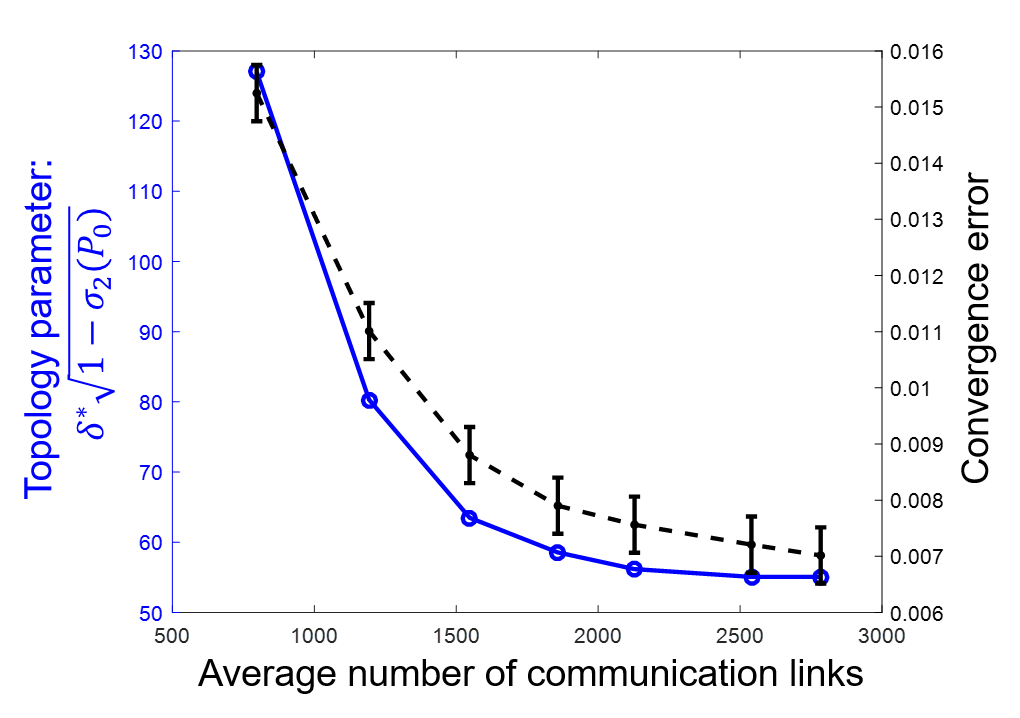
(a) (b)

Figure 4: Illustration of the optimal mixing time: a) solution path against $\beta$, b) mixing time and convergence error (regret) versus number of edges (communication links).

In Fig. 5, we present the regret versus the communication cost consumed during DDA with $T=20000$ and $\Delta=1$. For comparison, we present the predicted function error in Theorem 2 that is scaled up to constant factor. As we can see, there is a good agreement between the empirical function error and the theoretical prediction. Moreover, we show the number of added edges versus the communication cost consumed during DDA. In Fig. 5-(a), we show the behavior of the solution of problem (13) for different values of $\gamma$. Note that, consistent with consistent with Fig. 4-(b), the value of adding more edges diminishes when the total number of edges increases above the $50\%$ sparsity level.

(a) (b)

Figure 5: Function error at $T=20000$ versus the communication cost when $\Delta=1$: a) edge selection scheme provided by the solution of problem (13); b) edge selection scheme provided by the solution of problem (16).

In Fig. 5-(b), we present the function error by solving problem (16) under a fixed number of selected edges, $k=1377$. Compared to Fig. 5-(a), the communication cost increases due to edge rewiring rather than edge addition. However, the improvement on the function error of DDA is less significant. This implies that the number of scheduled edges plays a key role on the acceleration of DDA.

In Fig. 6, we present the empirical convergence time of DDA for different values of topology switching interval $\Delta$ in (74). Here the empirical convergence time is averaged over $20$ trials, the accuracy tolerance is chosen as $\epsilon=0.1$, and the edge selection scheme is given by the solution problem (13) at $\gamma=0.01$. For comparison, we plot the theoretical prediction of the lower bound on the convergence time in Proposition 3, and the number of scheduled edges while performing DDA. As we can see, the convergence time increases as $\Delta$ increases since the network connectivity grows faster, evidenced by the increase of scheduled edges. Moreover, we observe that the convergence behavior of DDA is improved significantly even under a relatively large $\Delta$, e.g., $\Delta=100$, compared to that of using a static network at $\Delta=20000$. This result implies that one can accelerate the convergence of DDA even in the regime of low switching rate through network topology design. Lastly, we note that the variation of the empirical convergence behavior is predicted well by our theoretical results in Proposition 3.

Figure 6: Convergence steps to $\epsilon$-accuracy solution versus topology switching interval $\Delta$.

Real-world application: distributed estimation over a sensor network

In what follows, we consider an application of distributed estimation based on temperature data collected across $32$ weather stations at $K=10$ sampling points [62]. The estimation problem is given by [39, Sec. IV-C]

$$\begin{array}[]{ll}\displaystyle\operatorname*{\text{minimize}}_{\mathbf{x}}&\frac{1}{n}\sum_{i=1}^{n}\left(\sum_{t=1}^{K}\|y_{i,t}-\mathbf{b}_{i}^{T}\mathbf{x}\|_{2}^{2}\right)+\mathcal{I}(\mathbf{x}),\end{array}$$ (76)

where $\mathbf{x}$ denotes the vector of temperature intensities to be estimated at some points in space, $y_{i,t}$ is the temperature observation at station $i$ and time $t$, $\{\mathbf{b}_{i}\}$ are observation vectors inferred from the past sensor observations and parameter estimate using the method in [62], and $\mathcal{I}(\mathbf{x})$ is an indicator function, $\mathcal{I}(\mathbf{x})=0$ if $\|\mathbf{x}\|_{2}\leq 5$, and $0$ otherwise. Since problem (76) contains the particular smooth+nonsmooth composite objective function, a proximal gradient exact first-order algorithm (PG-EXTRA) [14] and a distributed linearized alternating direction method of multipliers (DL-ADMM) [33] can be used for distributed estimation, with a linear convergence rate faster than DDA. Note that PG-EXTRA and DL-ADMM were defined under static networks while our approach is proposed for evolving networks of growing connectivity. In a fair comparison, we determine an equivalent-static network by solving the network design problem (16), so that the number of edges of this static network is the same as the average number of edges of the proposed time-evolving network.

In Fig. 7, we present the limiting regret as a function of the average number of communication links utilized by DDA. As we can see, PG-EXTRA and DL-ADMM outperform the DDA-based algorithms. This is not surprising, since both PG-EXTRA and L-ADMM have a linear convergence rate, faster than DDA. Specifically, the former utilizes historical information to obtain a better gradient estimate, and the latter uses the operator splitting method to accelerate the convergence rate. However, the performance gap between DDA and PG-EXTRA (or DL-ADMM) decreases as the number of communication links increases. We further note that when applied to the time varying network topology, DDA has better performance than that of using the equivalent-static network. In Fig. 8, we compare convergence trajectories when the avarage number of edges is $138$ and $200$, respectively. As we can see, the convergence speed is accelerated when the number of communication links increases. We also note that our approach converges slower at the beginning, however, it accelerates after a certain number of iterations due to the growing network connectivity. This leads to a $18\%$ improvement in the objective function at the end of the time horizon.

Figure 7: Regret against average number of communication links.

(a) (b)

Figure 8: Convergence trajectory at different number of communication links: a) 138 and b) 200.

VII Conclusions

In this paper, we studied the DDA algorithm for distributed convex optimization in multi-agent networks. We took into account the impact of network topology design on the convergence analysis of DDA. We showed that the acceleration of DDA is achievable under evolving networks of growing connectivity, where the growing networks can be designed via edge selection and scheduling. We demonstrated the tight connection between the improvement in convergence rate and the growth speed of network connectivity, which is absent in the existing analysis. Numerical results showed that our theoretical predictions are well matched to the empirical convergence behavior of accelerated DDA. There are multiple directions for future research. We would like to study the convergence rate of DDA when the network connectivity grows in average but not monotonically. It will also be of interest to address the issues of communication delays and link failures in the accelerated DDA algorithm. Last but not the least, we would relax the assumption of deterministically time-varying networks to randomly varying networks.

Appendix A Proof of Proposition 1

If $u_{t}=0$, we obtain $\lambda_{n-1}(\mathbf{L}_{t})=\lambda_{n-1}(\mathbf{L}_{t-1})$ from (17). In what follows, we consider the case of $u_{t}=1$. Let $d$ denote a lower bound on $\lambda_{n-1}(\mathbf{L}_{t})$, namely, $d\leq\lambda_{n-1}(\mathbf{L}_{t})$. By setting $\epsilon\mathrel{\mathop{:}}=d-\lambda_{n-1}(\mathbf{L}_{t-1})$, it has been shown in [44, Eq. 12] that the desired $\epsilon$ satisfies

$$\frac{c^{2}}{\epsilon}\geq 1+\frac{2}{\delta-\epsilon},$$ (77)

where $c\mathrel{\mathop{:}}=\mathbf{a}_{l_{t}}^{T}\mathbf{v}_{t-1}$, $\delta\mathrel{\mathop{:}}=\lambda_{n-2}(\mathbf{L}_{t-1})-\lambda_{n-1}(\mathbf{L}_{t-1})$, and $\delta-\epsilon=\lambda_{n-2}(\mathbf{L}_{t-1})-d\geq\lambda_{n-2}(\mathbf{L}_{t-1})-\lambda_{n-1}(\mathbf{L}_{t})>0$.

Multiplying (77) by $\epsilon(\delta-\epsilon)$ on both sides, we have

$$\epsilon^{2}-(c^{2}+2+\delta)\epsilon+c^{2}\delta\geq 0,$$ (78)

which implies that $\epsilon\geq\frac{x+\sqrt{x^{2}-y}}{2}$ or $\epsilon\in[0,\frac{x-\sqrt{x^{2}-y}}{2}]$, where $x=c^{2}+2+\delta$, and $y=4c^{2}\delta$.

For the case of $\epsilon\in[0,\frac{x-\sqrt{x^{2}-y}}{2}]$, since

$$(x-\sqrt{x^{2}-y})^{2}=2x^{2}-y-2x\sqrt{x^{2}-y}\geq 0,$$ (79)

we then obtain

$$\frac{y}{4x}\leq\frac{x-\sqrt{x^{2}-y}}{2}.$$ (80)

Due to $[0,\frac{y}{4x}]\subset[0,\frac{x-\sqrt{x^{2}-y}}{2}]$ implied by (80), we select $\epsilon=\frac{y}{4x}$ that satisfies (78). That is,

$$\epsilon=\frac{y}{4x}=\frac{c^{2}\delta}{c^{2}+2+\delta}=\frac{c^{2}}{\frac{c^{2}}{\delta}+\frac{2}{\delta}+1}.$$ (81)

Moreover, we have

$$c^{2}=(\mathbf{a}_{l_{t}}^{T}\mathbf{v}_{t-1})^{2}\leq\|\mathbf{a}_{l_{t}}\|_{2}^{2}\|\mathbf{v}_{t-1}\|_{2}^{2}\leq 4,$$ (82)

where we have used the fact that $[\mathbf{a}_{l_{t}}]_{i}=1$, $[\mathbf{a}_{l_{t}}]_{j}=-1$ and $0$s elsewhere for the $l_{t}$th edge in $\mathcal{E}_{\mathrm{selt}}$ that connects nodes $i$ and $j$.

Based on (81) and (82), we have

$$\epsilon=\frac{c^{2}}{\frac{c^{2}}{\delta}+\frac{2}{\delta}+1}\geq\frac{c^{2}}{\frac{6}{\delta}+1},$$ (83)

which yields

$$\lambda_{n-1}(\mathbf{L}_{t})\geq\lambda_{n-1}(\mathbf{L}_{t-1})+\frac{c^{2}}{\frac{6}{\delta}+1}.$$ (84)

Recalling the definitions of $c$ and $\delta$, we finally obtain (56). The proof is now complete. $\blacksquare$

Appendix B Derivation of Inequality (62)

Substituting (60) into (59), the term $\bar{\mathbf{z}}(t)-\mathbf{z}_{i}(t)$ becomes

$$\bar{\mathbf{z}}(t)-\mathbf{z}_{i}(t)= \sum_{s=1}^{t-1}\sum_{j=1}^{n}\left(\frac{1}{n}-[\bm{\Phi}(t-1,s)]_{ji}\right)\mathbf{g}_{j}(s-1)$$

$$+\sum_{j=1}^{n}\frac{1}{n}\mathbf{g}_{j}(t-1)-\mathbf{g}_{i}(t-1).$$ (85)

Since $f_{i}$ is $L$-Lipschitz continuous, we have $\|\mathbf{g}_{i}(t)\|_{*}\leq L$ for all $i$ and $t$, and

$$\|\bar{\mathbf{z}}(t)-\mathbf{z}_{i}(t)\|_{*} \leq L\sum_{s=1}^{t-1}\left\|\bm{\Phi}(t-1,s)\mathbf{e}_{i}-\mathbf{1}/n\right\|_{1}+2L,$$ (86)

where $\mathbf{e}_{i}$ is a basis vector with $1$ at the $i$th coordinate, and $0$s elsewhere. For a doubly stochastic matrix $\bm{\Phi}(t-1,s)$, we have the following inequality [9, 64]

$$\|\bm{\Phi}(t-1,s)\mathbf{e}_{i}-\mathbf{1}/n\|_{1}\leq\sigma_{2}(\bm{\Phi}(t-1,s))\sqrt{n}.$$ (87)

Based on (86) and (87), we obtain (62). $\blacksquare$

Appendix C Proof of Lemma 1

Since $\bm{\Phi}(t,s)$ is doubly stochastic, we have $\sigma_{1}(\bm{\Phi}(t,s))=\lambda_{1}(\bm{\Phi}(t,s))=1$ [64, Ch. 8]. The singular value decomposition of ${\bm{\Phi}}(t,s)$ is given by

$$\bm{\Phi}(t,s)=\mathbf{U}\bm{\Gamma}\mathbf{V}^{T}=\sum_{i=1}^{n}\sigma_{i}\mathbf{u}_{i}\mathbf{v}_{i}^{T},$$

where $\sigma_{1}=1$, and $\mathbf{u}_{1}=\mathbf{v}_{1}=\mathbf{1}/\sqrt{n}$.

Consider a matrix deflation $\tilde{\bm{\Phi}}(t,s)=\bm{\Phi}(t,s)-\mathbf{1}\mathbf{1}^{T}/n$, we have $\sigma_{1}(\tilde{\bm{\Phi}}(t,s))=\sigma_{2}(\bm{\Phi}(t,s))$. Based on [65, Theorem 9], we then obtain

$$\sigma_{1}\left(\tilde{\bm{\Phi}}(t,s+1)\tilde{\mathbf{P}}_{s}\right)\leq\sigma_{1}(\tilde{\bm{\Phi}}(t,s+1))\sigma_{1}(\tilde{\mathbf{P}}_{s}),$$ (88)

where $\tilde{\mathbf{P}}_{s}=\mathbf{P}_{s}-\mathbf{1}\mathbf{1}^{T}/n$, and

$$\tilde{\bm{\Phi}}(t,s+1)\tilde{\mathbf{P}}_{s}= [\bm{\Phi}(t,s+1)-\mathbf{1}\mathbf{1}^{T}/n][{\mathbf{P}}_{s}-\mathbf{1}\mathbf{1}^{T}/n]$$

$$= {\bm{\Phi}(t,s+1)\mathbf{P}_{s}}-\mathbf{1}\mathbf{1}^{T}/n=\bm{\Phi}(t,s)-\mathbf{1}\mathbf{1}^{T}/n$$

$$= \tilde{\bm{\Phi}}(t,s),~{}\text{for all $s\leq t$.}$$

From (88), we obtain $\sigma_{1}\left(\tilde{\bm{\Phi}}(t,s)\right)\leq\prod_{i=s}^{t}\sigma_{1}(\tilde{\mathbf{P}}_{i})$, which is equivalent to (63).

Appendix D Proof of Proposition 2

Let $\delta\mathrel{\mathop{:}}=t-s+1$, from (9) and (64) we have

$$\prod_{k={s}}^{t}\sigma_{2}(\mathbf{P}_{k}) \leq\prod_{k={0}}^{\delta-1}\sigma_{2}(\mathbf{P}_{k})$$

$$\leq\prod_{k={0}}^{\delta-1}\left[\sigma_{2}(\mathbf{P}_{0})-\sum_{i=1}^{k}u_{i}b_{i-1}(\mathbf{a}_{l_{i}}^{T}\mathbf{v}_{i-1})^{2}\right],$$ (89)

which yields

$$\prod_{k={0}}^{\delta-1}\frac{\sigma_{2}(\mathbf{P}_{k})}{\sigma_{2}(\mathbf{P}_{0})}\leq\prod_{k={0}}^{\delta-1}\left(1-\frac{\sum_{i=1}^{k}u_{i}b_{i-1}(\mathbf{a}_{l_{i}}^{T}\mathbf{v}_{i-1})^{2}}{\sigma_{2}(\mathbf{P}_{0})}\right).$$ (90)

Next, we introduce a variable $\beta$ defined as

$$\beta\mathrel{\mathop{:}}=\prod_{k={0}}^{\delta-1}\left(1-\frac{\sum_{i=1}^{k}u_{i}b_{i-1}(\mathbf{a}_{l_{i}}^{T}\mathbf{v}_{i-1})^{2}}{\sigma_{2}(\mathbf{P}_{0})}\right),$$ (91)

where by convention, $\beta=1$ if $\delta=1$.

Let $(\beta^{*},\delta^{*})$ be the solution of problem (66), we have

$$\delta^{*}\geq\frac{\log{T\sqrt{n}}}{\log{\sigma_{2}(\mathbf{P}_{0})^{-1}}}-\frac{\log{{\beta^{*}}^{-1}}}{\log{\sigma_{2}(\mathbf{P}_{0})^{-1}}}.$$ (92)

Based on (89) and (92), for any $\delta\geq\delta^{*}$ we have

$$\prod_{i={s}}^{t}\sigma_{2}(\mathbf{P}_{i})\leq\prod_{i={0}}^{\delta^{*}-1}\sigma_{2}(\mathbf{P}_{i})\leq\beta^{*}\sigma_{2}(\mathbf{P}_{0})^{\delta^{*}}\leq\frac{1}{T\sqrt{n}},$$ (93)

where the last inequality is equivalent to (92).

We split the right hand side of (86) at time $\delta^{*}$, and obtain

$$\|\bar{\mathbf{z}}(t)-\mathbf{z}_{i}(t)\|_{*}\leq L\sum_{s=1}^{t-1-\delta^{*}}\left\|\bm{\Phi}(t-1,s)\mathbf{e}_{i}-\mathbf{1}/n\right\|_{1}$$

$$+L\sum_{s=t-\delta^{*}}^{t-1}\left\|\bm{\Phi}(t-1,s)\mathbf{e}_{i}-\mathbf{1}/n\right\|_{1}+2L.$$ (94)

Since $\left\|\bm{\Phi}(t-1,s)\mathbf{e}_{i}-\mathbf{1}/n\right\|_{1}\leq 2$, the second term at the right hand side of (94) yields the following upper bound that is independent of $t$,

$$L\sum_{s=t-\delta^{*}}^{t-1}\left\|\bm{\Phi}(t-1,s)\mathbf{e}_{i}-\mathbf{1}/n\right\|_{1}\leq 2L\delta^{*}$$ (95)

Moreover, based on (87) and (63), the first term at the right hand side of (94) yields

$$L\sum_{s=1}^{t-1-\delta^{*}}\left\|\bm{\Phi}(t-1,s)\mathbf{e}_{i}-\mathbf{1}/n\right\|_{1}\leq L\sqrt{n}\sum_{s=1}^{t-1-\delta^{*}}\prod_{i={s}}^{t-1}\sigma_{2}(\mathbf{P}_{i})$$

$$\leq L\sqrt{n}\sum_{s=1}^{t-1-\delta^{*}}\prod_{i={t-1-\delta^{*}}}^{t-1}\sigma_{2}(\mathbf{P}_{i})\leq L\sqrt{n}\sum_{s=1}^{t-1-\delta^{*}}\prod_{i={0}}^{\delta^{*}-1}\sigma_{2}(\mathbf{P}_{i})$$

$$\leq L\sqrt{n}\sum_{s=1}^{t-1-\delta^{*}}\frac{1}{T\sqrt{n}},$$ (96)

where the last inequality holds due to (93), and $\sum_{s=1}^{t-1-\delta^{*}}\frac{1}{T}\leq 1$.

Substituting (95) and (96) into (92), we obtain

$$\|\bar{\mathbf{z}}(t)-\mathbf{z}_{i}(t)\|_{*} \leq 3L+2L\delta^{*}.$$ (97)

Substituting (97) into (59), we obtain (65). $\blacksquare$

Appendix E Proof of Corollary 3

Since $t_{i}\leq\hat{t}_{i}$ when $u_{t_{i}}=\hat{u}_{\hat{t}_{i}}=1$, at a particular time $t$ we have $\sum_{k=1}^{t}u_{k}\geq\sum_{k=1}^{t}\hat{u}_{k}$. Upon defining

$$\beta\mathrel{\mathop{:}}=\prod_{k={0}}^{\hat{\delta}^{*}-1}\left(1-\frac{\sum_{j=1}^{k}u_{j}b_{j-1}(\mathbf{a}_{l_{j}}^{T}\mathbf{v}_{j-1})^{2}}{\sigma_{2}(\mathbf{P}_{0})}\right),$$

we have

$$\beta\leq\prod_{k={0}}^{\hat{\delta}^{*}-1}\left(1-\frac{\sum_{j=1}^{k}\hat{u}_{j}b_{j-1}(\mathbf{a}_{l_{j}}^{T}\mathbf{v}_{j-1})^{2}}{\sigma_{2}(\mathbf{P}_{0})}\right)=\hat{\beta}^{*}.$$

Therefore, $\hat{\delta}^{*}\geq\frac{\log{T\sqrt{n}}}{\log{\sigma_{2}(\mathbf{P}_{0})^{-1}}}-\frac{\log{(\hat{\beta}^{*})^{-1}}}{\log{\sigma_{2}(\mathbf{P}_{0})^{-1}}}\geq\frac{\log{T\sqrt{n}}}{\log{\sigma_{2}(\mathbf{P}_{0})^{-1}}}-\frac{\log{(\beta)^{-1}}}{\log{\sigma_{2}(\mathbf{P}_{0})^{-1}}}$. This implies that the pair $(\beta,\hat{\delta}^{*})$ is a feasible point to problem (66) under the schedule $\{u_{t}\}$. Therefore, $\delta^{*}\leq\hat{\delta}^{*}$. $\blacksquare$

Appendix F Proof of Theorem 2

Based on Theorem 1, we obtain

$$f(\hat{\mathbf{x}}_{i}(T))-f(\mathbf{x}^{*})\leq \frac{1}{T\alpha_{T}}\psi(\mathbf{x}^{*})+\frac{L^{2}}{2T}\sum_{t=1}^{T}\alpha_{t-1}$$

$$+\sum_{t=1}^{T}\frac{L^{2}\alpha_{t}}{T}\left(6\delta^{*}+9\right).$$ (98)

Let $\alpha_{t}=a/\sqrt{t}$ with convention $\alpha_{0}=\alpha_{1}$ for some constant $a$. And applying $\sum_{t=1}^{T}t^{-1/2}\leq 2\sqrt{T}$ and $\psi(\mathbf{x}^{*})\leq R^{2}$ into (98), we obtain

$$f(\hat{\mathbf{x}}_{i}(T))-f(\mathbf{x}^{*})\leq\frac{R^{2}}{a\sqrt{T}}+\frac{aL^{2}}{\sqrt{T}}\left(12\delta^{*}+19\right).$$ (99)

Substituting $a={R\sqrt{1-\sigma_{2}(\mathbf{P}_{0})}}/{L}$ into (99), we obtain (69). $\blacksquare$

Appendix G Proof of Proposition 3

From (66a), we obtain

$$\beta\geq\left(1-\frac{\sum_{i=1}^{\ell}b_{i-1}(\mathbf{a}_{l_{i}}^{T}\mathbf{v}_{i-1})^{2}}{\sigma_{2}(\mathbf{P}_{0})}\right)^{\delta},$$ (100)

where $\ell$ is the number of scheduled edges. Substituting (100) into (66b), we obtain

$$\delta\geq\frac{\log{T\sqrt{n}}}{\log{\sigma_{2}(\mathbf{P}_{0})^{-1}}}-\frac{\delta\log{\alpha^{-1}}}{\log{\sigma_{2}(\mathbf{P}_{0})^{-1}}},$$ (101)

which yields

$$\delta^{*}\geq\frac{\log{T\sqrt{n}}}{\log{\sigma_{2}(\mathbf{P}_{0})^{-1}}+\log{\alpha^{-1}}},$$ (102)

where $\delta^{*}$ is the optimal solution of problem (66), $\alpha\mathrel{\mathop{:}}=1-\frac{\sum_{i=1}^{\ell}b_{i-1}(\mathbf{a}_{l_{i}}^{T}\mathbf{v}_{i-1})^{2}}{\sigma_{2}(\mathbf{P}_{0})}$, and $\alpha\in[0,1]$ due to (64).

To find the convergence time for the desired $\epsilon$-accuracy, consider the following inequality suggested by Theorem 2,

$$\frac{RL\sqrt{1-\sigma_{2}(\mathbf{P}_{0})}}{\sqrt{T}}\delta^{*}\leq\epsilon.$$ (103)

Substituting (102) into (103), we obtain a necessary condition to bound the convergence time

$$\frac{RL\sqrt{1-\sigma_{2}(\mathbf{P}_{0})}}{\sqrt{T}}\frac{1}{\log{\sigma_{2}(\mathbf{P}_{0})^{-1}}+\log{\alpha^{-1}}}\leq\epsilon.$$ (104)

Since $\log{(\sigma_{2}(\mathbf{P}_{0})^{-1}\alpha^{-1})}\geq 1-\sigma_{2}(\mathbf{P}_{0})\alpha$, it is sufficient to consider

$$\frac{RL\sqrt{1-\sigma_{2}(\mathbf{P}_{0})}}{\sqrt{T}}\frac{1}{1-\sigma_{2}(\mathbf{P}_{0})\alpha}\leq\epsilon,$$ (105)

which yields

$$T=\Omega\left(\frac{1}{\epsilon^{2}}\frac{1-\sigma_{2}(\mathbf{P}_{0})}{(1-\sigma_{2}(\mathbf{P}_{0})\alpha)^{2}}\right).$$ (106)

The proof is now complete. $\blacksquare$

References

- [1] B. Hendrickson and T. G. Kolda, “Graph partitioning models for parallel computing,” Parallel computing, vol. 26, no. 12, pp. 1519–1534, 2000.
- [2] A. Pothen, “Graph partitioning algorithms with applications to scientific computing,” in Parallel Numerical Algorithms, pp. 323–368. Springer, 1997.
- [3] D. Blatt, A. O. Hero, and H. Gauchman, “A convergent incremental gradient method with a constant step size,” SIAM Journal on Optimization, vol. 18, no. 1, pp. 29–51, 2007.
- [4] R. Olfati-Saber, J. A. Fax, and R. M. Murray, “Consensus and cooperation in networked multi-agent systems,” Proceedings of the IEEE, vol. 95, no. 1, pp. 215–233, Jan. 2007.
- [5] F. P Kelly, A. K Maulloo, and D. K. H Tan, “Rate control for communication networks: shadow prices, proportional fairness and stability,” Journal of the Operational Research Society, vol. 49, no. 3, pp. 237–252, 1998.
- [6] M. Chiang, S. H. Low, A. R. Calderbank, and J. C. Doyle, “Layering as optimization decomposition: A mathematical theory of network architectures,” Proceedings of the IEEE, vol. 95, no. 1, pp. 255–312, Jan. 2007.
- [7] O. L. Mangasarian, “Mathematical programming in neural networks,” ORSA Journal on Computing, vol. 5, no. 4, pp. 349–360, 1993.
- [8] F. Dörfler, M. Chertkov, and F. Bullo, “Synchronization in complex oscillator networks and smart grids,” Proceedings of the National Academy of Sciences, vol. 110, no. 6, pp. 2005–2010, 2013.
- [9] J. C. Duchi, A. Agarwal, and M. J. Wainwright, “Dual averaging for distributed optimization: Convergence analysis and network scaling,” IEEE Transactions on Automatic Control, vol. 57, no. 3, pp. 592–606, March 2012.
- [10] D. Jakovetić, J. Xavier, and J. M. F. Moura, “Fast distributed gradient methods,” IEEE Transactions on Automatic Control, vol. 59, no. 5, pp. 1131–1146, May 2014.
- [11] D. Jakovetić, J. M. F. Xavier, and J. M. F. Moura, “Convergence rates of distributed nesterov-like gradient methods on random networks,” IEEE Transactions on Signal Processing, vol. 62, no. 4, pp. 868–882, Feb. 2014.
- [12] W. Shi, Q. Ling, G. Wu, and W. Yin, “Extra: An exact first-order algorithm for decentralized consensus optimization,” SIAM Journal on Optimization, vol. 25, no. 2, pp. 944–966, 2015.
- [13] G. Qu and N. Li, “Harnessing smoothness to accelerate distributed optimization,” IEEE Transactions on Control of Network Systems, 2017.
- [14] W. Shi, Q. Ling, G. Wu, and W. Yin, “A proximal gradient algorithm for decentralized composite optimization,” IEEE Transactions on Signal Processing, vol. 63, no. 22, pp. 6013–6023, 2015.
- [15] Y. Nesterov, “Primal-dual subgradient methods for convex problems,” Mathematical Programming, vol. 120, no. 1, pp. 221–259, 2009.
- [16] S. Hosseini, A. Chapman, and M. Mesbahi, “Online distributed admm on networks,” arXiv preprint arXiv:1412.7116, 2014.
- [17] T. Suzuki, “Dual averaging and proximal gradient descent for online alternating direction multiplier method,” in International Conference on Machine Learning, 2013, pp. 392–400.
- [18] F. R. K. Chung, Spectral Graph Theory, American Mathematical Society, Dec. 1996.
- [19] R. Olfati-Saber and R. M. Murray, “Consensus problems in networks of agents with switching topology and time-delays,” IEEE Transactions on Automatic Control, vol. 49, no. 9, pp. 1520–1533, Sept. 2004.
- [20] Y. Hatano and M. Mesbahi, “Agreement over random networks,” IEEE Transactions on Automatic Control, vol. 50, no. 11, pp. 1867–1872, Nov. 2005.
- [21] L. Xiao and S. Boyd, “Fast linear iterations for distributed averaging,” Systems and Control Letters, vol. 53, pp. 65–78, 2003.
- [22] S. Kar and J. M. F. Moura, “Distributed consensus algorithms in sensor networks with imperfect communication: Link failures and channel noise,” IEEE Transactions on Signal Processing, vol. 57, no. 1, pp. 355–369, Jan. 2009.
- [23] A. Nedić, A. Olshevsky, A. Ozdaglar, and J. N. Tsitsiklis, “On distributed averaging algorithms and quantization effects,” IEEE Transactions on Automatic Control, vol. 54, no. 11, pp. 2506–2517, Nov. 2009.
- [24] S. Y. Tu and A. H. Sayed, “Diffusion strategies outperform consensus strategies for distributed estimation over adaptive networks,” IEEE Transactions on Signal Processing, vol. 60, no. 12, pp. 6217–6234, Dec. 2012.
- [25] A. Koppel, B. M. Sadler, and A. Ribeiro, “Proximity without consensus in online multi-agent optimization,” https://arxiv.org/abs/1606.05578, 2016.
- [26] J. Tsitsiklis, D. Bertsekas, and M. Athans, “Distributed asynchronous deterministic and stochastic gradient optimization algorithms,” IEEE Transactions on Automatic Control, vol. 31, no. 9, pp. 803–812, Sept. 1986.
- [27] A. Nedić and A. Ozdaglar, “Distributed subgradient methods for multi-agent optimization,” IEEE Transactions on Automatic Control, vol. 54, no. 1, pp. 48–61, Jan. 2009.
- [28] I. Lobel and A. Ozdaglar, “Distributed subgradient methods for convex optimization over random networks,” IEEE Transactions on Automatic Control, vol. 56, no. 6, pp. 1291–1306, June 2011.
- [29] S. Sundhar Ram, A. Nedić, and V. V. Veeravalli, “Distributed stochastic subgradient projection algorithms for convex optimization,” Journal of Optimization Theory and Applications, vol. 147, no. 3, pp. 516–545, 2010.
- [30] D. Jakovetic, D. Bajovic, N. Krejic, and N. K. Jerinkic, “Distributed gradient methods with variable number of working nodes.,” IEEE Trans. Signal Processing, vol. 64, no. 15, pp. 4080–4095, 2016.
- [31] A. Mokhtari, Q. Ling, and A. Ribeiro, “Network newton distributed optimization methods,” IEEE Transactions on Signal Processing, vol. 65, no. 1, pp. 146–161, Jan. 2017.
- [32] E. Wei and A. Ozdaglar, “On the convergence of asynchronous distributed alternating direction method of multipliers,” in 2013 IEEE Global Conference on Signal and Information Processing, Dec. 2013, pp. 551–554.
- [33] N. S. Aybat, Z. Wang, T. Lin, and S. Ma, “Distributed linearized alternating direction method of multipliers for composite convex consensus optimization,” IEEE Transactions on Automatic Control, 2017.
- [34] Y. Nesterov, “A method of solving a convex programming problem with convergence rate ,” Soviet Mathematics Doklady, vol. 27, pp. 372–376, 1983.
- [35] K. I. Tsianos and M. G. Rabbat, “Distributed dual averaging for convex optimization under communication delays,” in Proc. 2012 American Control Conference (ACC), June 2012, pp. 1067–1072.
- [36] K. I. Tsianos, S. Lawlor, and M. G. Rabbat, “Push-sum distributed dual averaging for convex optimization,” in Proc. 51st IEEE Conference on Decision and Control (CDC), Dec. 2012, pp. 5453–5458.
- [37] D. Yuan, S. Xu, H. Zhao, and L. Rong, “Distributed dual averaging method for multi-agent optimization with quantized communication,” Systems & Control Letters, vol. 61, no. 11, pp. 1053 – 1061, 2012.
- [38] S. Lee, A. Nedić, and M. Raginsky, “Coordinate dual averaging for decentralized online optimization with nonseparable global objectives,” IEEE Transactions on Control of Network Systems, vol. PP, no. 99, pp. 1–1, 2016.
- [39] S. Hosseini, A. Chapman, and M. Mesbahi, “Online distributed convex optimization on dynamic networks,” IEEE Transactions on Automatic Control, vol. 61, no. 11, pp. 3545–3550, Nov 2016.
- [40] S. Liu, P.-Y. Chen, and A. O. Hero, “Distributed optimization for evolving networks of growing connectivity,” in Proc. IEEE International Conference on Acoustics, Speech and Signal Processing (ICASSP). IEEE, 2017, pp. 4079–4083.
- [41] B. Smith, P. Bjorstad, and W. Gropp, Domain decomposition: parallel multilevel methods for elliptic partial differential equations, Cambridge university press, 2004.
- [42] D. Xue, A. Gusrialdi, and S. Hirche, “A distributed strategy for near-optimal network topology design,” in Proc. 21th International Symposium on Mathematical Theory of Networks and Systems, 2014, pp. 7–14.
- [43] P.-Y. Chen and A. O. Hero, “Assessing and safeguarding network resilience to nodal attacks,” IEEE Communications Magazine, vol. 52, no. 11, pp. 138–143, Nov. 2014.
- [44] A. Ghosh and S. Boyd, “Growing well-connected graphs,” in Proceedings of the 45th IEEE Conference on Decision and Control, Dec. 2006, pp. 6605–6611.
- [45] S. Boyd, “Convex optimization of graph laplacian eigenvalues,” in International Congress of Mathematicians, 2006, pp. 1311–1319.
- [46] David A. Levin, Yuval Peres, and Elizabeth L. Wilmer, Markov chains and mixing times, American Mathematical Society, 2006.
- [47] M. Fiedler, “Algebraic connectivity of graphs,” Czechoslovak Mathematical Journal, vol. 23, no. 2, pp. 298–305, 1973.
- [48] L. Shi, P. Cheng, and J. Chen, “Optimal periodic sensor scheduling with limited resources,” IEEE Transactions on Automatic Control, vol. 56, no. 9, pp. 2190–2195, Sept. 2011.
- [49] V. Gupta, T. Chung, B. Hassibi, and R. M. Murray, “Sensor scheduling algorithms requiring limited computation,” in Proceedings of IEEE International Conference on Acoustics, Speech, and Signal Processing, 2004, vol. 3, pp. 825–828.
- [50] V. Gupta, T. H. Chung, B. Hassibi, and R. M. Murray, “On a stochastic sensor selection algorithm with applications in sensor scheduling and sensor coverage,” Automatica, vol. 42, no. 2, pp. 251–260, 2006.
- [51] X. Zhao, “The laplacian eigenvalues of graphs: A survey,” https://arxiv.org/abs/1111.2897, 2011.
- [52] S. Boyd and L. Vandenberghe, Convex Optimization, Cambridge University Press, Cambridge, 2004.
- [53] F. Bach, R. Jenatton, J. Mairal, and G. Obozinski, “Optimization with sparsity-inducing penalties,” Found. Trends Mach. Learn., vol. 4, no. 1, pp. 1–106, Jan. 2012.
- [54] A. Nemirovski, “Interior point polynomial time methods in convex programming,” 2012 [Online], Available: http://www2.isye.gatech.edu/~nemirovs/Lect_IPM.pdf.
- [55] S. Boyd, L. Xiao, and A. Mutapcic, “Subgradient methods,” Notes for EE392o, Stanford University, Autumn, 2003, Available: https://web.stanford.edu/class/ee392o/subgrad_method.pdf.
- [56] N. Parikh and S. Boyd, “Proximal algorithms,” Foundations and Trends in Optimization, vol. 1, no. 3, pp. 123–231, 2013.
- [57] F. Iutzeler, P. Ciblat, and J. Jakubowicz, “Analysis of max-consensus algorithms in wireless channels,” IEEE Transactions on Signal Processing, vol. 60, no. 11, pp. 6103–6107, Nov. 2012.
- [58] J. He, P. Cheng, L. Shi, J. Chen, and Y. Sun, “Time synchronization in wsns: A maximum-value-based consensus approach,” IEEE Transactions on Automatic Control, vol. 59, no. 3, pp. 660–675, March 2014.
- [59] S. Liu, P.-Y. Chen, and A. O. Hero, “Accelerated distributed dual averaging over evolving networks of growing connectivity,” arXiv preprint arXiv:1704.05193, 2017.
- [60] A. Nemirovski and D. Yudin, Problem Complexity and Method Efficienc in Optimization, New York: Wiley, 1983.
- [61] E. Hazan, “Introduction to online convex optimization,” Foundations and Trends® in Optimization, vol. 2, no. 3-4, pp. 157–325, 2016.
- [62] S. P. Chepuri, S. Liu, G. Leus, and A. O. Hero, “Learning sparse graphs under smoothness prior,” in Proc. 2017 IEEE International Conference on Acoustics, Speech and Signal Processing (ICASSP). IEEE, 2017, pp. 6508–6512.
- [63] N. Perraudin, J. Paratte, D. I. Shuman, V. Kalofolias, P. Vandergheynst, and D. K. Hammond, “Gspbox: A toolbox for signal processing on graphs,” Aug. 2014 [Online], Available: http://arxiv.org/abs/1408.5781.
- [64] R. A. Horn and C. R. Johnson, Matrix analysis, Cambridge University Press, Cambridge, U.K., 1985.
- [65] J. K. Merikoski and R. Kumar, “Inequalities for spreads of matrix sums and products,” in Applied Mathematics E-Notes, 2004, pp. 150–159.