Satellite Based Positioning Signal Acquisition at Higher Order Cycle Frequency

Abstract

The acquisition of the signal from the satellite based positioning systems, such as GPS, Galileo, and Compass, encounters challenges in the urban streets, indoor. For improving the acquisition performance, the data accumulation is usually performed to improve the signal-to-noise ratio which is defined on the second order statistics. Different from the conventional approaches, the acquisition based on higher order cyclostatistics is proposed. Using the cyclostatistics, the estimation of the initial phase and Doppler shift of the signal is presented respectively. Afterwards, a joint estimator is introduced. The analysis in this paper is performed on GPS signal. Indeed, the proposed estimation method can be straightforwardly extended to acquire the signal from the other satellite positioning systems. The simulation and experiment results demonstrate that the proposed signal acquisition scheme achieves the detection probability of 0.9 at the CNR 28dBHz.

I Introduction

With the extension satellites based positioning and navigation service, the GPS receiver encounters the problem of the signal acquisition in the challenging environments, such as indoor, on urban street and in woods with dense leaves [1]. In these environments, the GPS signal becomes weak and can hardly be acquired by the receivers. To solve the problem, the studies on the weak GPS signal acquisition methods are widely performed. Generally, these GPS signal acquisition methods can be divided into two main categories. First, piling up GPS data is adopted to increase SNR [2, 3, 4, 5, 6]. Second, mitigating the interference from the noise, the jamming signal and the unexpected GPS signals [7, 8, 9] is another approach to improving GPS signal acquisition performance.

Coherent accumulation is a classical method of acquiring weak GPS signal acquisition. Even though the SNR increases with the extending accumulated GPS signal length, the coherently accumulated signal length does not goes beyond 10ms due to the data bit transition. To improve the SNR furthermore, Psiaki [2] studied two non-coherent GPS signal accumulation methods, ‘full-bit’ and ‘half-bit’ GPS signal acquisition methods, which noncoherently pile up the GPS data to improve the GPS signal acquisition performance. In the condition that the carrier-to-noise (CNR) is larger than zero, the GPS signal noncoherent accumulation will generate the higher SNR. However, the accumulated GPS data duration can not be extended without limits. The noncoherent GPS signal accumulation will induce square loss; and the Doppler shift will also limit the accumulated GPS signal length extension. Thus, the GPS signal acquisition performance improvement by the noncoherent GPS signal accumulation is limited. At the direction of increasing SNR by piling up the GPS data, differential coherent accumulation method is also employed [3, 4]. The differential coherent accumulation based acquisition method sums up the products of two adjacent coherent results. The GPS signal acquisition method increases the Doppler shift tolerance which is also insensitive to the data bit transition. Thus for differential coherent accumulation the constraint on the GPS signal data length extension is not so strict as the coherent accumulation which length is shorter than 10ms in usual cases. However, the shortage of the differential coherent accumulation is obvious that the SNR gain efficiency is not high enough compared with coherent accumulation method in the condition of the small Doppler shift.

Wang etc. [7] employed the noise subspace tracking algorithm to reduce the degradation from the interference which is a kind of spatial filtering method. The noise subspace tracking method depends on an antenna array to implement beam forming to mitigate the interference. Inevitably, the antenna array will increase the cost of the GPS receiver. Morton etc. [8] studied the GPS signal self-interference mitigation method by subspace projection. However, in the study of Morton, the non-orthogonality between the different GPS signal is neglected of, that is, the cross-correlation result between different pseudorandom codes is not exact zero. Huang and Pi [9] studied the interference between the different GPS signals which is called the near-far effect in GPS signal acquisition. Three different kinds of solutions to the near-far problem are proposed. Unfortunately, there is no one general method which can handle all the three kinds of the near-far problems. Besides that, the coexistence of multiplicative and additive noise in GPS signal is deeply studied [10].

Huang etc. [11] proposed a GPS signal detection algorithm which employed Duffing chaotic oscillator to detect the weak GPS signals. The GPS signal detection algorithm utilizes the immunity to noise and sensitivity to the periodical signals. GPS signal has two periods possessed by the carrier and the pseudorandom code. Meanwhile, the noise is of no any periodicity in usual cases. The external periodical force from the periodic input signal will change the state of the chaotic oscillator by which the GPS signal is detected. However, there is a gap between the algorithm study and the hardware implementation since the chaotic oscillator based GPS signal acquisition method demands for the quite heavy computation burden. Also, Liu etc. [12] and Sahmoudi etc. [13] studied the degraded GPS signal tracking algorithm in the challenging environments with dense multipath and jamming signal. As we know, the tracking algorithm in the challenging environments makes sense only after the weak GPS signal is successfully acquired. The studies on improving hardware of GPS receiver are performed in [14, 15, 16]. The mobile states assisted positioning performance improvement is studied in [17].

Indeed, the GPS signal possesses cyclostationary feature which enables the GPS receiver distinguish the expected GPS signal from the background noise and jamming signal. To the best knowledge of the author, few publications refers to utilizing the cyclostastionary feature to acquire the weak GPS signal.

In the 1950s, cyclostationary feature was proposed to characterize the statistics which is non-stationary but periodic. Since the 1980s Gardner W.A. has performed wide and deep research work on the cyclostatistics and the related applications [18, 19, 20, 21, 22, 23, 24]. Until now, there are huge amount of signal processing algorithms based on cyclostatistics in the various fields. However, as the author can refer, there is no publication on GPS signal detection based on the cyclostationary feature.

In this paper, the cyclostationary feature of the GPS signal is analyzed firstly; after that, the GPS signal detection method based on cyclostatistics is proposed and the detection performance is analyzed; also the initial pseudorandom code phase and the Doppler shift estimation methods are studied; in the end part of this article the simulations and experiments are carried out to test the effectiveness of the proposed GPS signal acquisition scheme.

II Cyclostationary Feature and Cyclic Spectrum of GPS Signal Equations

The GPS signal is represented by $s(t)$. The $s(t)$ is the time period of 1ms is given by

$$g(t)=\sum_{k=0}^{1022}c(k)q(t-kT_{c}-t_{0})\cos(2\pi f_{0}t+\theta_{0}).$$ (1)

where $T_{c}$ denotes the time duration of one pseudorandom code chip. $q(t)$ is the square wave with duration, $q(t)=1$ for $0\leq t\leq T_{c}$, otherwise, $q(t)=0$. $t_{0}$ is the initial pseudorandom code phase. $f_{0}$ is the signal carrier frequency. $\theta_{0}$ is the initial phase of the carrier.

To investigate the cyclostationary feature of GPS signal, we calculate the mean and the variance of $s(t)$

In one period of C/A code, due to ergodic feature, the mean value of $s(t)$ is approximately calculated by

$$M_{s} =\int_{0}^{T_{0}}s(t)dt$$ (2)

$$=\int_{0}^{T_{0}}\sum_{k=0}^{1022}c(k)q(t-kT_{c}-t_{0})\cos(2\pi f_{0}t+\theta_{0})dt$$

$$\approx 0,$$

where $T_{0}$ denotes the period of C/A code.

The autocorrelation of the GPS signal $s(t)$ is written as

$$R_{s}(t,\tau) =\int_{t}^{t+\Delta t}s(t)s(t+\tau)dt$$ (3)

Since $s(t)$ is periodic at the period of $T_{0}$, that is, $s(t+T_{0})=s(t)$, we have

$$R_{s}(t+T_{0},\tau)_{\Delta t} =\int_{t}^{t+\Delta t}s(t+T_{0})s(t+T_{0}+\tau)dt$$ (4)

$$=\int_{t}^{t+\Delta t}s(t)s(t+\tau)dt$$

$$=R_{s}(t,\tau)_{\Delta t}$$

Based the results in the previous several steps, the mean value of GPS signal is constant and autocorrelation function is periodic versus time. Therefore, GPS signal is cyclostationary. The derivation is according to the definition by Gardner. Because of the periodicity in the GPS signal autocorrelation function, Fourier series of the periodic function can be calculated as follows,

$$R_{s}(t,\tau) =\sum_{n=-\infty}^{+\infty}R_{G}^{\frac{n}{T_{0}}}(\tau)e^{j2\pi\frac{n}{T_{0}}t}$$ (5)

where $\frac{n}{T_{0}}$ is the cyclic frequency, $n\in\mathbb{Z}$ and

$$R_{G}^{\frac{n}{T_{0}}}(\tau)=\int_{\Delta t}R_{G}(t,\tau)e^{-j2\pi\frac{n}{T_{0}}t}dt$$ (6)

For derivation convenience, let $\alpha$ denote the cyclic frequency, $\alpha=\frac{n}{T_{0}}$. $R_{G}^{\frac{n}{T_{0}}}(\tau)$ is thecyclic-autocorrelation function at cyclic frequency at $\alpha$. According to the definition, the cyclic spectrum, denoted by $S_{G}^{\alpha}(f)$, is calculated as follows,

$$S_{G}^{\alpha}(f)=\int R_{G}(t,\tau)e^{-j2\pi f\tau}dt$$ (7)

Until now, the background of cyclostatistics and the cyclostationary feature of GPS signal are introduced. Next, we will present the cyclostatistics based initial code phase estimation method.

III Cyclic-spectrum Based Initial Code Phase Estimation

To successfully acquire GPS signal, we need to obtain the two information, initial pseudorandom code phase and the Doppler shift. As the prime acquisition taks, initial phase estimation based on cyclicspectrum is introduced in this section.

III-A Conventional Initial PN Code Phase Estimation

Remember $g(t)$ denotes the ideal GPS signal. The received one is denoted by $r(t)$. Let $\tau$ denote the pseudorandom (PN) phase difference between $g(t)$ and $r(t)$ and $\tau<|T_{0}|$. With the definitions, the received signal $r(t)$ is written as follows

$$r(t)=A\cdot g(t-D)+\xi(t)$$ (8)

The conventional initial phase estimation is based on the peak detection on the correlation between the ideal signal $g(t)$ and the received one $r(t)$. The correlation can be straightforwardly obtained as follows,

$$R_{R,G}(\tau)=A\cdot R_{G}(\tau-D)+R_{\Xi,G}(t,\tau).$$ (9)

To implement the peak detection, we smoothly change the value of $\tau$ within the duration of $T_{0}$. Since the noise $\xi$ is uncorrelated with the signal $g(t)$, $R_{\Xi,G}$ approaches to zero in the high SNR case. Thus, the correlation $R_{R,G}$ is determined by the autocorrelation function $R_{G}$. When $\tau=D$, $R_{G}$ reaches the maximum value, so $R_{R,G}$ does. The peak detection is completed.

The conventional acquisition method can easily implemented. However, when GPS encounters severely degraded noise, $R_{\Xi,G}$ no longer approaches to zero; thus the autocorrelation result will submerge in the background noise and the peak detection can not be successfully achieved.

III-B Initial Phase Estimation Method Based on Cyclic-spectrum Correlation

As shown previously, GPS signal is cyclostationary, while the noise does not. In the interference channel, jamming signal might be cyclostationary or not. Even for cyclostationary jamming signal, its cyclostationarity is different from that of the expected GPS signal. Therefore, we are able to detect the GPS signal from the background with strong noise and interference. Concretely speaking, the cyclic-spectrum is utilized to estimate the initial PN code phase.

Let $g^{\prime}(t)$ denote the replica of $g(t)$ with a phase shift $\delta$, that is, $g^{\prime}(t)=g(t-\delta)$. $S_{G^{\prime},G}^{\alpha}(f)$ denotes the cyclic-spectrum calculated from $g(t)$ and $g^{\prime}(t)$, and $S_{R,G}^{\alpha}(f)$ denotes the cyclic-spectrum calculated from the received signal $r(t)$ and $g(t)$. The cyclic-spectrum $S_{R,G}^{\alpha}$ is calculated by

$$S_{R,G}^{\alpha}(f)=\mathcal{F}\left\{R_{R,G}^{\alpha}(\tau)\right\}$$ (10)

$$=\mathcal{F}\left\{\lim_{T\rightarrow\infty}\frac{1}{T}\int_{-T}^{T}\left(\begin{matrix}(g(t-D+\frac{\tau}{2})+\xi(t))\\ \cdot g^{*}(t-\frac{\tau}{2})\end{matrix}\right)e^{-j2\pi\alpha t}dt\right\}$$

$$\overset{(a)}{=}\mathcal{F}\left\{\lim_{T\rightarrow\infty}\frac{1}{T}\int_{-T}^{T}\left(\begin{matrix}g(t-\frac{D}{2}+\left(\frac{\tau}{2}-\frac{\tau}{2}\right))\\ \cdot g^{*}(t-\frac{D}{2}-\left(\frac{\tau}{2}-\frac{\tau}{2}\right))\end{matrix}\right)e^{-j2\pi\alpha t}dt\right\}$$

$${=}\mathcal{F}\left\{R^{\alpha}_{G}(\tau-D)e^{-j\pi\alpha D}\right\}$$

$${=}S^{\alpha}_{G}(f)e^{-j2\pi\left(\frac{\alpha}{2}+f\right)D}$$

where $(a)$ follows that the cyclostatistic of noise is zero when $\alpha\neq 0$.

Similarly, we calculate $S_{G^{\prime},G}^{\alpha}$ which is listed as follows,

$$S_{G^{\prime},G}^{\alpha}(f)=S^{\alpha}_{G}(f)e^{-j2\pi\left(\frac{\alpha}{2}+f\right)\delta}$$ (11)

The similarity between the two cyclic-spectrum is calculated to complete the estimation of the initial PN code phase. Let $D_{ec}$ denote the similarity which is calculated as follows,

$$D_{ec} =\int_{-\infty}^{\infty}{S_{G^{\prime},G}^{\alpha}(f)}^{*}S_{R,G}^{\alpha}(f)df$$ (12)

$$=\int_{-\infty}^{\infty}|S_{G}^{\alpha}(f)|^{2}e^{-j2\pi\left(\frac{\alpha}{2}+f\right)\left(\delta-D\right)}df$$

From (12), when

$$-j2\pi\left(\frac{\alpha}{2}+f\right)\left(\delta-D\right)\rightarrow 0,$$ (13)

$D_{ec}$ approaches the maximum. According to the result, the initial pseudorandom code phase delay $D$ can be obtained by calculating the maximum absolute value of the cyclic-spectrum correlation.

Until now, the theoretic proof on the initial phase delay estimation based on the cyclic-spectrum is completed. However, the calculation performed in the derivation is far from a practical case. Next, we will propose a practical scheme to implement the cyclic-spectrum based initial phase estimation.

III-C Practical Scheme of the Cyclic-spectrum Based Initial Phase Estimation

According to the definition, the cyclostatistics $R_{R,G}^{\alpha}(\tau)$ is calculated by

$$R_{R,G}^{\alpha}(\tau)=\lim_{T\rightarrow\infty}\frac{1}{T}\int_{-\frac{T}{2}}^{\frac{T}{2}}\left(\begin{matrix}(r(t+\frac{\tau}{2})e^{-j\pi\alpha\left(t+\frac{\tau}{2}\right)})\\ \cdot(g(t-\frac{\tau}{2})e^{-j\pi\alpha\left(t-\frac{\tau}{2}\right)})\end{matrix}\right)dt$$ (14)

According to the previous analysis results, $R_{R,G}^{\alpha}(\tau)$ is periodic at the period of $T_{0}$. The cyclic-spectrum $S_{R,G}^{\alpha}(f)$ is calculated as follows,

$$S_{R,G}^{\alpha}(f)=\frac{1}{T_{0}}\int_{T_{0}}R_{R,G}^{\alpha}(\tau)e^{-j2\pi\tau f}d\tau$$ (15)

$$=\frac{1}{T_{0}}\int_{T_{0}}\frac{1}{T}\lim_{T\rightarrow\infty}\int_{t-\frac{T}{2}}^{t+\frac{T}{2}}\left(\begin{matrix}(r(\zeta+\frac{\tau}{2})e^{-j\pi\alpha\left(\zeta+\frac{\tau}{2}\right)})\\ \cdot(g(\zeta-\frac{\tau}{2})e^{-j\pi\alpha\left(\zeta-\frac{\tau}{2}\right)})\end{matrix}\right)d\zeta e^{-j2\pi\tau f}d\tau$$

$$=\lim_{T\rightarrow\infty}\frac{1}{T}\int_{t-\frac{T}{2}}^{t+\frac{T}{2}}\frac{1}{T_{0}}\int_{T_{0}}\left(\begin{matrix}(r(\zeta+\frac{\tau}{2})e^{-j\pi\alpha\left(\zeta+\frac{\tau}{2}\right)})\\ \cdot(g(\zeta-\frac{\tau}{2})e^{-j\pi\alpha\left(\zeta-\frac{\tau}{2}\right)})\end{matrix}\right)d\tau e^{-j2\pi\tau f}d\zeta$$

$$=\lim_{T\rightarrow\infty}\frac{1}{T}\int_{t-\frac{T}{2}}^{t+\frac{T}{2}}\frac{1}{T_{0}}\int_{T_{0}}\left(\begin{matrix}\left(r(\zeta+\frac{\tau}{2})e^{-j\pi\left(\frac{\alpha}{2}+f\right)\left(\zeta+\frac{\tau}{2}\right)}\right)\\ \cdot\left(g(\zeta-\frac{\tau}{2})e^{-j\pi\left(-\frac{\alpha}{2}+f\right)\left(\zeta-\frac{\tau}{2}\right)}\right)^{*}\end{matrix}\right)d\tau d\zeta$$

$$=\lim_{T\rightarrow\infty}\frac{1}{T}\int_{-\infty}^{\infty}\frac{1}{T_{0}}\int_{T_{0}}\left(\begin{matrix}(r(\zeta+\frac{\tau}{2})e^{-j\pi\left(\frac{\alpha}{2}+f\right)\left(\zeta+\frac{\tau}{2}\right)})\\ \cdot(g(\zeta-\frac{\tau}{2})e^{-j\pi\left(-\frac{\alpha}{2}+f\right)\left(\zeta-\frac{\tau}{2}\right)})^{*}\end{matrix}\right)d\tau d\zeta$$

$$~{}~{}~{}~{}~{}\cdot\otimes rec_{T}(t)$$

where

$$rec_{T}(a)=\left\{\begin{matrix}\frac{1}{T},&|a|\leq\frac{T}{2}\\ 0,&|a|>\frac{T}{2}\end{matrix}\right.$$ (16)

For derivation simplicity, we define two auxiliary variables, $R_{T_{0}}(t,f)$ and $G_{T_{0}}(t,f)$ as follows,

$$R_{T_{0}}(t,f)=\frac{1}{\sqrt{T_{0}}}\int_{T_{0}}r(t+\frac{\tau}{2})e^{-j2\pi(\frac{\alpha}{2}+f)(t+\frac{\tau}{2})}d\tau\otimes rec_{T}(t)$$ (17)

$$=R_{T_{0}}^{\prime}(t,f+\frac{\alpha}{2}),$$

and

$$G_{T_{0}}(t,f)=\frac{1}{\sqrt{T_{0}}}\int_{T_{0}}r(t+\frac{\tau}{2})e^{-j2\pi(\frac{-\alpha}{2}+f)(t-\frac{\tau}{2})}d\tau\otimes rec_{T}(t)$$ (18)

$$=G_{T_{0}}^{\prime}(t,f-\frac{\alpha}{2}),$$

where

$$R_{T_{0}}^{\prime}(t,f)=\frac{1}{\sqrt{T_{0}}}\int_{t}^{t+T_{0}}r(\zeta)e^{-j2\pi f\zeta}d\zeta$$ (19)

$$G_{T_{0}}^{\prime}(t,f)=\frac{1}{\sqrt{T_{0}}}\int_{t}^{t+T_{0}}g(\zeta)e^{-j2\pi f\zeta}d\zeta$$

Substituting (17) and (18) into (15), we have the cyclic-spectrum as follows,

$$S_{R,G}^{\alpha}(f) =\lim_{T\rightarrow\infty}\frac{1}{T}\int_{-\frac{T}{2}}^{\frac{T}{2}}R_{T_{0}}(t,f){G_{T_{0}}(t,f)}^{*}dt\otimes rec_{T}(t)$$ (20)

$$=\lim_{T\rightarrow\infty}\frac{1}{T}\int_{-\frac{T}{2}}^{\frac{T}{2}}R_{T_{0}}^{\prime}(t,f){G_{T_{0}}^{\prime}(t,f)}^{*}dt$$

Now, the practical scheme in analog time domain is presented. For the application in the widely used digital circuits, we next transform the analog practical scheme into discrete time form. In the discrete time domain, the cyclic-spectrum is calculated as follows,

$$S_{R,GD}^{\alpha}[m]=\lim_{N\rightarrow\infty}\frac{1}{N}\sum_{n=1}^{N}R_{T_{0}D}[n,m]{G_{T_{0}D}[n,m]}^{*}$$ (21)

$$= \lim_{N\rightarrow\infty}\frac{1}{N}\sum_{n=1}^{N}R_{T_{0}D}^{\prime}\left[n,m+\frac{\Phi}{2}\right]{G_{T_{0}D}^{\prime}\left[n,m-\frac{\Phi}{2}\right]}^{*}$$

$$= \lim_{N\rightarrow\infty}\frac{1}{N}\sum_{n=1}^{N}\left(\begin{matrix}\left(\frac{1}{\sqrt{M}}\sum_{m=n+1}^{n+M}r[n]e^{-j2\pi(m+\frac{\Phi}{2})pt_{s}}\right)\\ \cdot{\left(\frac{1}{\sqrt{M}}\sum_{m=n+1}^{n+M}g[n]e^{-j2\pi(m-\frac{\Phi}{2})pt_{s}}\right)}^{*}\end{matrix}\right)$$

where $f_{s}$ is the sampling frequency and $t_{s}$ is the sampling period; $\Phi$ denotes the shift in the frequency domain caused by cyclic frequency $\alpha$ which is calculated by $\Phi=2\cdot floor\left(\frac{\alpha}{2f_{s}}\right)$.

For a more intuitive understanding on the practical scheme, we present a block diagram of the practical cyclic-spectrum based initial phase estimation scheme. The block diagram is shown in Fig. 1

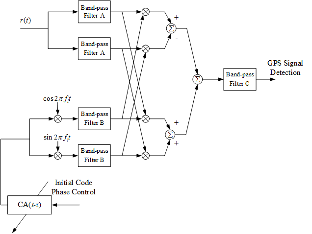
Figure 1: GPS signal acquisition block diagram based on cyclic-spectrum correlation

In Fig. 1, the central frequency of the band-pass filter A is located at $\frac{\alpha}{2}+f$ with bandwidth of $\Delta f$; the central frequency of the band-pass filter B is located at $-\frac{\alpha}{2}+f$ with bandwidth $\Delta f$; the central frequency of band-pass filter C is located at $\alpha$ with bandwidth of $\frac{1}{\Delta t}$.

In processing shown in Fig. 1, to alleviate the frequency leaking problem, frequency smoothing is performed. The bandwidth of the frequency smoothing window is equal to $\Delta f$. We define $I$ as,

$$I=\left\lfloor\frac{\Delta f}{f_{s}}\right\rfloor.$$ (22)

Let $\tilde{S}_{R,GD}^{\alpha}[m]$ denote the cyclic-spectrum after the smoothing operation which is calculated as follows,

$$\tilde{S}_{R,GD}^{\alpha}[m]=\frac{1}{N}\sum_{n=1}^{N}\frac{1}{I}\sum_{i=-\frac{I-1}{2}}^{\frac{I-1}{2}}\left(\begin{matrix}(R_{T_{0}D}^{\prime}\left[n,m+\frac{\Phi}{2}+i\right])\\ \cdot({G_{T_{0}D}^{\prime}\left[n,m-\frac{\Phi}{2}+i\right]}^{*})\end{matrix}\right)$$ (23)

(a) GPS signal cyclic-spectrum before smoothing

(b) GPS signal cyclic-spectrum after smoothing

Figure 2: GPS signal cyclic-spectrum smoothing demo

Fig. 2(a) and Fig. 2(b) illustrate the cyclic-spectrum of the GPS signal before and after the frequency smoothing. From Fig. 2, we can observe the frequency leaking problem is released after the smoothing operation.

III-D Initial PN Code Phase Iterative Estimation Scheme

The block processing based initial phase estimation method is presented in the previous subsection. The block operation requires the large duration of data which generates processing delay. To solve the problem, we propose a iterative structure based initial phase estimation scheme in this subsection.

Remember that the received GPS signal in the discrete time domain is written as $r[n]=g[n-D]+\xi[n]$. According to the conclusion in [25], $g[n-D]$ can be approximately expanded by a set of sinc functions as follows,

$$g[n-D]=\sum_{i=-P}^{P}sinc(i-D)g[n-i],$$ (24)

where $sinc(x)$ is equal to $\frac{\sin(x)}{x}$ for $x\neq 0$ and 1 for $x=0$; $P$ is a positive integer larger than $D$.

We calculate the cyclostatistics from $r[n]$ and $g[n]$ as follows,

$$R_{R,G}^{\alpha}[n_{\tau}]=\left<\left(g[n-D]+\xi[n]\right)g[n-n_{\tau}]e^{-j2\pi\alpha nt_{s}}\right>_{\Delta t},$$ (25)

where $\left<\cdot\right>_{\Delta t}=\frac{1}{\Delta t}\int_{\Delta t}$; $\Delta t$ is equal to the data length in the calculation, $\Delta t=N\cdot t_{s}$; and $n=\lfloor\frac{\tau}{t_{s}}\rfloor$.

The noise $\xi$ is not cyclostationary for $\alpha\geq 1$. Thus, we have $R_{\Xi,G}^{\alpha}=0$ and $R_{R,G}^{\alpha}$ is rewritten as follows,

$$R_{R,G}^{\alpha}[n_{\tau}]=\left<g[n-D]g[n-n_{\tau}]e^{-j2\pi\alpha nt_{s}}\right>_{\Delta t},$$ (26)

Substituting (24) into (26), we have

$$R_{R,G}^{\alpha}[n_{\tau}]=\left<\begin{matrix}\\ \left(\sum_{i=-P}^{P}sinc(i-D)g[n+\frac{n_{\tau}}{2}-i]\right)\\ \cdot e^{-j\pi\alpha nt_{s}}g[n-\frac{n_{\tau}}{2}]e^{-j\pi\alpha nt_{s}}\end{matrix}\right>_{\Delta t}$$ (27)

$$=\sum_{i=-P}^{P}\left(\begin{matrix}sinc(i-D)e^{-j\pi\alpha it_{s}}\\ \cdot\left<g[n+\frac{n_{\tau}}{2}-i]e^{-j\pi\alpha(n-i)t_{s}}g[n-\frac{n_{\tau}}{2}]e^{-j\pi\alpha nt_{s}}\right>_{\Delta t}\end{matrix}\right)$$

$$=\sum_{i=-P}^{P}sinc(i-D)e^{-j\pi\alpha it_{s}}R_{G}^{\alpha}[n_{\tau}-i],$$

Next, we define the cost function built on the cyclostatistics as follows,

$$\varepsilon(k,n_{\tau})= R_{R,G}^{\alpha}[n_{\tau}]$$ (28)

$$- \sum_{i=-P}^{P}sinc(i-\hat{D}[k])e^{-j\pi\alpha it_{s}}R_{G}^{\alpha}[n_{\tau}-i],$$

where $\hat{D}[k]$ denotes the estimation of the phase delay $D$ after $k$-th iterative computation.

From (28), we have the square of the cost function as follows,

$$J=\sum_{n_{\tau}=-N_{\tau}}^{N_{\tau}}|\varepsilon(k,n_{\tau})|^{2},$$ (29)

Next, we calculate the derivate function of $J$ versus the estimated initial PN code phase delay $\hat{D}[k]$,

$$\hat{\nabla}[k]=\frac{\partial J}{\partial\hat{D}[k]}$$ (30)

$$=2\sum_{n_{\tau}=-N_{\tau}}^{N_{\tau}}\varepsilon(k,n_{\tau})\sum_{i=-P}^{P}f\left(i-\hat{D}[k]\right)R_{G}^{\alpha}[n_{\tau}-i],$$

where $f(x)=\frac{\cos(\pi x)-sinc(x)}{x}$ and $N_{\tau}$ is the maximum initial phase shift.

Afterwards, we have the iterative code phase estimation method which is under the rule of minimum square error. The method is shown below,

$$\hat{D}[k+1]=\hat{D}[k]-\mu\hat{\nabla}[k],$$ (31)

where $\mu$ is the step in the iterative computation.

To present a intuitive impression, Fig. 3 illustrates the block diagram of the iterative estimator.

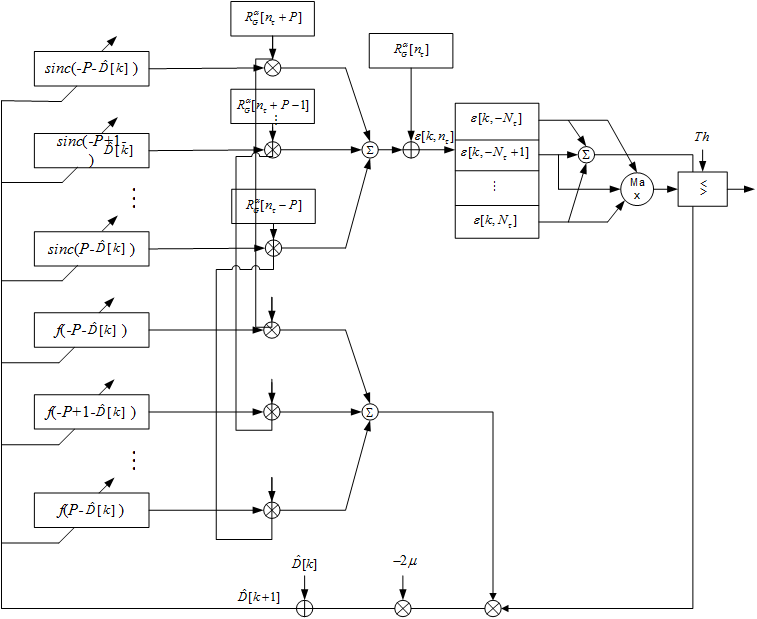
Figure 3: Iterative initial phase estimation block diagram

IV Doppler Shift Estimation Based on Cyclic-spectrum

For analysis simplicity, we first consider the GPS signal with Doppler shift, but no phase delay. From such an ideal signal, we estimate the Doppler using a cyclic-spectrum based method. In the next section, we will extend the method to acquire the practical GPS signal which is with both Doppler shift and phase delay.

Still, let $r(t)$ denote the GPS signal which is written as follows,

$$r(t)=g(t)e^{j2\pi f_{d}t}+\xi(t),$$ (32)

where $f_{d}$ is equal to the Doppler shift value.

IV-A Conventional Doppler Estimation Method

The conventional Doppler shift estimation is based on measuring the similarity between $r(t)$ signal $l(t)$ with respect to the second order statistics. With the consideration of the periodicity of PN code, the correlation function of GPS signal can be written as

$$R(t,\tau)=\frac{1}{T}\int_{t}^{t+T}\left[g(\zeta)e^{j2\pi f_{d}\zeta}+\xi{\zeta}\right]g(\zeta-\tau)e^{-j2\pi f_{d}(\zeta-\tau)}d\zeta,$$ (33)

where $T$ is $n$ times the PN code period, $T=n\times T_{0}$.

Since the GPS signal $g$ is uncorrelated with the noise $\xi$ and the mean of $\xi$ is zero,

$$R(t,\tau)=\frac{1}{T}\int_{t}^{t+T}g(\zeta)g(\zeta-\tau)e^{j2\pi(f_{d}-f_{dl})\zeta+j2\pi f_{dl}\tau}d\zeta,$$ (34)

Let $\Delta f$ denote the frequency difference between the Doppler shift $f_{d}$ and $f_{dl}$, $\Delta f=f_{d}-f_{dl}$. $R(t,\tau)$ is further derived as follows,

$$R(t,\tau)=\frac{1}{T}e^{j2\pi f_{dl}\tau}\int_{t}^{t+T}g(\zeta)g(\zeta-\tau)e^{j2\pi\Delta f\zeta}d\zeta$$ (35)

$$= \frac{1}{T}e^{j2\pi f_{dl}\tau}\int_{-\infty}^{\infty}\left(\begin{matrix}g(\zeta)g(\zeta-\tau)e^{j2\pi\Delta f\zeta}\\ \cdot(u(\zeta-t)-u(\zeta-t-T))\end{matrix}\right)d\zeta$$

$$\overset{(a)}{=} \frac{e^{j2\pi f_{dl}}\tau}{T}\int_{-\infty}^{\infty}\left(\begin{matrix}g(\zeta)g(\zeta-\tau)e^{j2\pi\Delta f\zeta}\\ \cdot(u(\zeta-t+\frac{T}{2})-u(\zeta-t-T-\frac{T}{2}))\end{matrix}\right)d\zeta$$

where $(a)$ follows the periodicity.

Furthermore, we straightforwardly find that

$$|R(t,\tau)|$$ (36)

$$= \frac{1}{T}\left|\int_{-\infty}^{\infty}\left(\begin{matrix}g(\zeta)g(\zeta-\tau)\\ \cdot(u(\zeta-t+\frac{T}{2})-u(\zeta-t-T-\frac{T}{2}))\end{matrix}\right)d\zeta\right|$$

$$= :|R(t,\tau)|_{max},$$

where the equality is achieved at $\Delta f=0$.

According to Parseval principle, we have

$$|R(t,\tau)|_{max}=\left|\int_{-\infty}^{\infty}G^{2}(f)sinc(fT)df\right|,$$ (37)

where $G(f)$ is the Fourier transform of $g(t)$.

In the sense of 3dB bandwidth ($B_{3dB}=\frac{0.6034}{T}$) for the sinc function, the equation above can be written as

$$|R(t,\tau)|_{max}\cong\frac{1}{2}\left|\int_{-B_{3dB}}^{B_{3dB}}G^{2}(f)df\right|,$$ (38)

In real cases, $\Delta f$ can not exactly be equal to zero, but very small value, $\Delta f\ll\frac{B_{3dB}}{100}$. Then, we have

$$|R(t,\tau)|_{max}= \frac{1}{2}\left|\int_{-\infty}^{\infty}G^{2}(f)\delta(f-\Delta f)sinc(fT)df\right|$$ (39)

$$\cong \left|\int_{-B_{3dB}}^{B_{3dB}}G^{2}(f-\Delta f)df\right|.$$

From (39), we can adjust the value of $f_{dl}$ to make it approach to $f_{d}$ such that $\Delta f$ becomes small. Since the small $\Delta$ induces the maximum absolute correlation value, the Doppler shift can be determined by searching the maximum value of $|R(t,\tau)|_{max}$.

IV-B Doppler Estimation Based on Cyclic-spectrum

In this subsection, we introduce a method of estimating Doppler based on the cyclostatistics of GPS signal. The cyclostatistic of the received signal at cyclic frequency $\alpha$ is calculated as follows,

$$R^{\alpha}_{R}(\tau)=\lim_{T\rightarrow\infty}\frac{1}{T}\int_{-\frac{T}{2}}^{\frac{T}{2}}r(\zeta+\frac{\tau}{2})r(\zeta-\frac{\tau}{2})e^{-j2\pi\alpha\zeta}d\zeta$$ (40)

$$=\lim_{T\rightarrow\infty}\frac{1}{T}\int_{-\frac{T}{2}}^{\frac{T}{2}}\begin{matrix}\left(\begin{matrix}\left(g(\zeta+\frac{\tau}{2})e^{-j2\pi f_{d}(\zeta+\frac{\tau}{2})}+\xi(\zeta+\frac{\tau}{2})\right)\\ \cdot\left(g(\zeta-\frac{\tau}{2})e^{-j2\pi f_{d}(\zeta-\frac{\tau}{2})}+\xi(\zeta-\frac{\tau}{2})\right)\end{matrix}\right)\\ \cdot e^{-j2\pi\alpha\zeta}d\zeta\end{matrix}$$

$$\overset{(a)}{=}\lim_{T\rightarrow\infty}\frac{1}{T}\int_{-\frac{T}{2}}^{\frac{T}{2}}g(\zeta+\frac{\tau}{2})g(\zeta-\frac{\tau}{2})e^{-j2\pi(\alpha-2f_{d})\zeta}d\zeta.$$

where $(a)$ follows that the cyclostatistics of the noise at high order cyclic frequency is equal to zero.

With the similar derivations, we calculate $R^{\alpha,G}_{R}(\tau)$ as follows,

$$R^{\alpha}_{R,G}(\tau)=\lim_{T\rightarrow\infty}\frac{1}{T}\int_{-\frac{T}{2}}^{\frac{T}{2}}\left(\begin{matrix}(g(\zeta+\frac{\tau}{2})g(\zeta-\frac{\tau}{2}))\\ \cdot e^{-j2\pi(\alpha-f_{d}-f_{dl})\zeta}\end{matrix}\right)d\zeta.$$ (41)

Afterwards, we calculate the correlation between the cyclostatistics $R^{\alpha}_{R,G}$ and $R^{\alpha}_{R}$ which is taken at the statistics used for Doppler estimation,

$$D_{ec}=\frac{1}{\Delta t}=\int_{\Delta t}R^{\alpha}_{R,G}(\tau){R^{\alpha}_{R}(\tau)}^{*}d\tau.$$ (42)

From (42), the absolute of $D_{ec}$ reaches the maximum at $f_{d}=f_{dl}$. Based on the results, we are able to calculate $D_{ec}$ at different $f_{dl}$’s and select the largest $|D_{ec}|$. The corresponding $f_{dl}$ is the estimation of $f_{d}$, that is,

$$\hat{f}_{d}=\arg\max_{f_{dl}}\{D_{ec}(f_{dl})\}.$$ (43)

V Joint Estimation of Initial PN Code Phase and Doppler Based on Cyclic-spectrum

In this section, the cyclic-spectrum of GPS signal is utilized to estimate the initial PN code phase and the Doppler shift in a joint way. Let $l(t)$ denote the locally generated GPS signal with a combination of configurable initial phase and Doppler shift. Let $R^{\alpha}_{R,L}(\tau)$ denote the cyclostatistics calculated from $r(t)$ and $l(t)$ at the cyclic frequency of $\alpha$. $R^{\alpha}_{R,L}(\tau)$ is calculated as follows,

$$R^{\alpha}_{R,L}(\tau)=\lim_{T\rightarrow\infty}\frac{1}{T}\int_{-\frac{T}{2}}^{\frac{T}{2}}r(\zeta+\frac{\tau}{2})l(\zeta-\frac{\tau}{2})e^{-j2\pi\alpha\zeta}d\zeta$$ (44)

$$=\lim_{T\rightarrow\infty}\frac{1}{T}\int_{-\frac{T}{2}}^{\frac{T}{2}}\left[g(\zeta+\frac{\tau}{2})+\xi(\zeta+\frac{\tau}{2})\right]l(\zeta-\frac{\tau}{2})e^{-j2\pi\alpha\zeta}d\zeta$$

$$\overset{(a)}{=}\lim_{T\rightarrow\infty}\frac{1}{T}\int_{-\frac{T}{2}}^{\frac{T}{2}}g(\zeta+\frac{\tau}{2})l(\zeta-\frac{\tau}{2})e^{-j2\pi\alpha\zeta}d\zeta$$

$$=\lim_{T\rightarrow\infty}\frac{1}{T}\int_{-\frac{T}{2}}^{\frac{T}{2}}\left(\begin{matrix}(g(\zeta+\frac{\tau}{2}-D)e^{j2\pi\alpha(\zeta+\frac{\tau}{2})})\\ \cdot(g(\zeta-\frac{\tau}{2}-\Theta)e^{j2\pi\alpha(\zeta-\frac{\tau}{2})})\end{matrix}\right)e^{-j2\pi\alpha\zeta}d\zeta$$

$$=\lim_{T\rightarrow\infty}\frac{1}{T}\int_{-\frac{T}{2}}^{\frac{T}{2}}\begin{matrix}\left(\begin{matrix}g(\zeta-\frac{D-\Theta}{2}+(\frac{\tau}{2}-\frac{D-\Theta}{2}))\\ \cdot g(\zeta-\frac{D-\Theta}{2}-(\frac{\tau}{2}-\frac{D-\Theta}{2}))\end{matrix}\right)\\ \cdot e^{j2\pi(f_{d}+f_{dl}-\alpha)\zeta}d(\zeta-\frac{D-\Theta}{2})\end{matrix}$$

$$=R_{G}^{f_{d}+f_{dl}-\alpha}(\tau-D-\Theta)e^{j2\pi(f_{d}+f_{dl}-\alpha)\frac{D-\Theta}{2}},$$

where $(a)$ follows that the cyclostatistics of the noise at high order cyclic frequency is equal to zero.

Similarly, the cyclostatistics $R_{R}^{\alpha}$ is calculated as follows,

$$R^{\alpha}_{R}(\tau)=\lim_{T\rightarrow\infty}\frac{1}{T}\int_{-\frac{T}{2}}^{\frac{T}{2}}r(\zeta+\frac{\tau}{2})r(\zeta-\frac{\tau}{2})e^{-j2\pi\alpha\zeta}d\zeta$$ (45)

$$=\lim_{T\rightarrow\infty}\frac{1}{T}\int_{-\frac{T}{2}}^{\frac{T}{2}}\left(\begin{matrix}(g(\zeta+\frac{\tau}{2}-D)e^{j2\pi\alpha(\zeta+\frac{\tau}{2})})\\ \cdot(g(\zeta-\frac{\tau}{2}-\Theta)e^{j2\pi\alpha(\zeta-\frac{\tau}{2})})\end{matrix}\right)e^{-j2\pi\alpha\zeta}d\zeta$$

$$=\lim_{T\rightarrow\infty}\frac{1}{T}\int_{-\frac{T}{2}}^{\frac{T}{2}}\begin{matrix}g(\zeta-D+\frac{\tau}{2})g(\zeta-D-\frac{\tau}{2})\\ \cdot e^{j2\pi(2f_{d}-\alpha)\zeta}d(\zeta-D)\end{matrix}$$

$$=R_{G}^{2f_{d}-\alpha}(\tau)e^{j2\pi(2f_{d}-\alpha)D}.$$

The corresponding cyclic-spectrum is calculated as follows,

$$S^{\alpha}_{R,L}(f)=\mathcal{F}\{R^{\alpha}_{R,L}(\tau)\}$$ (46)

$$=\mathcal{F}\{R^{f_{d}+f_{dl}-\alpha}_{G}(\tau-D-\Theta)e^{j2\pi(f_{d}+f_{dl}-\alpha)\frac{D-\Theta}{2}}\}$$

$$=S^{f_{d}+f_{dl}-\alpha}_{G}(f)e^{-j2\pi f(D-\Theta)}e^{j2\pi(f_{d}+f_{dl}-\alpha)\frac{D-\Theta}{2}},$$

and

$$S^{\alpha}_{R,L}(f)=\mathcal{F}\{R^{\alpha}_{R}(\tau)\}$$ (47)

$$=\mathcal{F}\{R^{f_{d}+f_{dl}-\alpha}_{G}(\tau)e^{j2\pi(2f_{d}-\alpha)D}\}$$

$$=S^{2f_{d}-\alpha}_{G}(f)e^{j2\pi(2f_{d}-\alpha)D}.$$

With the calculated cyclic-spectrum $S^{\alpha}_{R,L}$ and $S^{\alpha}_{R}$, we calculate the statistics used for joint estimation as follows,

$$\Lambda_{de}=\int_{-\infty}^{\infty}S^{\alpha}_{R,L}(f){S^{\alpha}_{R}}^{*}(f)df$$ (48)

$$=e^{j2\pi(f_{d}+f_{dl}-\alpha)\frac{D-\Theta}{2}}e^{j2\pi(2f_{d}-\alpha)D}$$

$$\cdot \int_{-\infty}^{\infty}S^{f_{d}+f_{dl}-\alpha}_{G}(f){S^{2f_{d}-\alpha}_{G}(f)}^{*}e^{-j2\pi f(D-\Theta)}df$$

The absolute value of $\Lambda_{dec}$,

$$|\Lambda_{de}|=\left|\int_{-\infty}^{\infty}S^{f_{d}+f_{dl}-\alpha}_{G}(f){S^{2f_{d}-\alpha}_{G}(f)}^{*}e^{-j2\pi f(D-\Theta)}df\right|,$$ (49)

is used for the peak searching.

From (49), we can achieve the GPS acquisition by peak searching the $|\Lambda_{de}|$ over the two dimensions of initial phase and Doppler. More concretely, we granularly change is value of $\Theta$ and $f_{dl}$ and calculate the corresponding $|\Lambda_{de}(\Theta,f_{dl})|$. At the maximum value, the initial phase delay and Doppler shift of the GPS signal are obtained,

$$(\hat{\Theta},\hat{f}_{dl})=\arg\max_{\Theta,f_{dl}}\{|\Lambda_{de}(\Theta,f_{dl})|\},$$ (50)

To test the cyclic-spectrum based GPS signal acquisition scheme, we first calculate the corresponding receiver operating characteristic curve (ROC) which is plotted in Fig. 4.

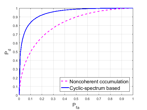
Figure 4: Receiver operating characteristic curve of the proposed cyclic-spectrum based GPS detection scheme

From Fig. 4, the cyclic-spectrum based GPS acquisition scheme has better ROC curve which is more convex than the one for correlation based detection scheme. The advantage is due to the fact that GPS signal is immune to noise at high order cyclic frequency.

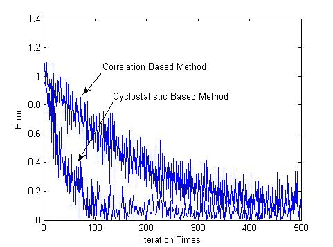
Figure 5: Error curve in iterative computations at 44dBHz

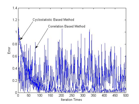
Figure 6: Error curve in iterative computations at 28dBHz

We also perform simulations to test the time delay estimation based on cyclic-spectrum of GPS signal which takes the form of iterative computation. Still, the correlation based data accumulation method is taken as the reference. In the experiment, the data length is equal to 20ms; iteration step is 0.03; sampling frequency is 5MHz. At the configuration, the corresponding value of $P$ is equals to 2500; the initial value of time delay $\hat{D}(0)$ is set to one.

Fig. 5 illustrates the error curve in the first 500 iteration times at the CNR of 44dBHz which corresponds to the LOS channel condition. From Fig. 5, both the conventional method and the cyclostatistics based one can achieve successful estimation in high SNR condition, while the cyclostatistic based method converges faster than the conventional one. Fig. 6 shows the results at CNR 26dBHz which corresponds to the channel condition with severe degradation. In Fig. 6, conventional method can not achieve the successful estimation on initial PN code phase while cyclostatistics based estimation method can.

Furthermore, to test the performance at more signal conditions, detection probabilities at different CNR are calculated and the results are plotted in Fig. 7. As a contrast, the noncoherent detection is also performed. In the experiments the threshold is set aiming at one false alarm among $10^{6}$ times experiments which guarantees the false alarm probability at $10^{-6}$.

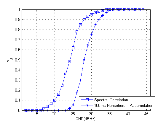
Figure 7: GPS signal detection performance comparison

From Fig. 7, the cyclic-spectrum based method outperforms the noncoherent accumulation based method. The detection probability of the cyclic-spectrum based method approaches 0.9 at 28dBHz CNR, while the conventional method based on the 100ms noncoherent accumulation approaches 0.9 at 32dB/Hz.

VI Conclusions

Since the mean of the GPS signal approaches zero and the correlation function is periodic, GPS signal is cyclostationary. We thus utilize the cyclostationary feature detect GPS signal acquisition at low CNR. Due to the non-cyclostationarity of Gaussian noise and the unconsistent cyclostationary feature of the jamming signal, the GPS signal can be distinguished from the background noise and the interference more easily.

The cyclostationary feature of the GPS signal is illustrated and the cyclic-spectrum of the GPS signal presented firstly;

We first introduce how to utilize the cyclic-spectrum to estimate initial phase of pseudorandom code and Doppler shift respectively. An iterative estimation scheme is also proposed. Afterwards, a joint estimation scheme is presented. The simulation results show that the cyclic-spectrum based method outperforms the conventional structure which is based on noncoherent accumulation.

References

• [1] J. B.-Y. Tsui, Acquisition of GPS C/A Code Signals.   John Wiley & Sons, Inc., 2001, pp. 133–164. [Online]. Available: http://dx.doi.org/10.1002/0471200549.ch7
• [2] M. L. Psiaki and A. P. Mechanical, “Block acquisition of weak gps signals in a software receiver,” in in Proc. of ION GPS, 2001.
• [3] H. Elders-Boll and U. Dettmar, “Efficient differentially coherent code/doppler acquisition of weak gps signals,” in Spread Spectrum Techniques and Applications, 2004 IEEE Eighth International Symposium on, Aug 2004, pp. 731–735.
• [4] W. Yu, B. Zheng, R. Watson, and G. Lachapelle, “Differential combining for acquiring weak gps signals,” Signal Process., vol. 87, no. 5, pp. 824–840, May 2007. [Online]. Available: http://dx.doi.org/10.1016/j.sigpro.2006.08.004
• [5] P.-D. Huang and Y.-m. PI, “Study on gps signal adaptive acquisition based on constant false alarm rate,” Acta Electronica Sinica, vol. 7, p. 042, 2011.
• [6] H. P. P. Yiming, “Study on constant false alarm rate gps signal detection based on differential accumulation [j],” Journal of Electronic Measurement and Instrument, vol. 1, p. 003, 2011.
• [7] R. Wang, M. Yao, Z. Cheng, and H. Zou, “Interference cancellation in {GPS} receiver using noise subspace tracking algorithm,” Signal Processing, vol. 91, no. 2, pp. 338 – 343, 2011. [Online]. Available: http://www.sciencedirect.com/science/article/pii/S0165168410003087
• [8] Y. Morton, M. Miller, J. Tsui, D. Lin, and Q. Zhou, “Gps civil signal self-interference mitigation during weak signal acquisition,” Signal Processing, IEEE Transactions on, vol. 55, no. 12, pp. 5859–5863, Dec 2007.
• [9] P. Huang and Y. Pi, “Urban environment solutions to gps signal near-far effect,” Aerospace and Electronic Systems Magazine, IEEE, vol. 26, no. 5, pp. 18–27, May 2011.
• [10] P. Huang, Y. Pi, and I. Progri, “Gps signal detection under multiplicative and additive noise,” Journal of Navigation, vol. 66, no. 04, pp. 479–500, 2013.
• [11] P. Huang, Y. Pi, and Z. Zhao, “Weak gps signal acquisition algorithm based on chaotic oscillator,” EURASIP Journal on Advances in Signal Processing, vol. 2009, no. 1, p. 862618, 2009. [Online]. Available: http://asp.eurasipjournals.com/content/2009/1/862618
• [12] L. Liu and M. G. Amin, “Tracking performance and average error analysis of {GPS} discriminators in multipath,” Signal Processing, vol. 89, no. 6, pp. 1224 – 1239, 2009. [Online]. Available: http://www.sciencedirect.com/science/article/pii/S0165168409000152
• [13] M. Sahmoudi and M. G. Amin, “Robust tracking of weak {GPS} signals in multipath and jamming environments,” Signal Processing, vol. 89, no. 7, pp. 1320 – 1333, 2009. [Online]. Available: http://www.sciencedirect.com/science/article/pii/S0165168409000036
• [14] P.-d. Huang and Y.-m. PI, “Research on gps signal acquisition based on cordic algorithm,” Gnss World of China, vol. 4, p. 006, 2009.
• [15] P. Huang and Y. Pi, “Saw based convolver for gps signal acquisition module,” Analog Integrated Circuits and Signal Processing, vol. 71, no. 1, pp. 111–117, 2012.
• [16] ——, “Research on novel structure of gps signal acquisition based on software receiver,” in Intelligent Signal Processing and Communication Systems (ISPACS), 2010 International Symposium on.   IEEE, 2010, pp. 1–4.
• [17] ——, “An improved location service scheme in urban environments with the combination of gps and mobile stations,” Wireless Communications and Mobile Computing, vol. 14, no. 13, pp. 1287–1301, 2014.
• [18] W. Gardner and L. Franks, “Characterization of cyclostationary random signal processes,” Information Theory, IEEE Transactions on, vol. 21, no. 1, pp. 4–14, Jan 1975.
• [19] W. Gardner, “The role of spectral correlation in design and performance analysis of synchronizers,” Communications, IEEE Transactions on, vol. 34, no. 11, pp. 1089–1095, Nov 1986.
• [20] ——, “Signal interception: a unifying theoretical framework for feature detection,” Communications, IEEE Transactions on, vol. 36, no. 8, pp. 897–906, Aug 1988.
• [21] W. Gardner and C.-K. Chen, “Interference-tolerant time-difference-of-arrival estimation for modulated signals,” Acoustics, Speech and Signal Processing, IEEE Transactions on, vol. 36, no. 9, pp. 1385–1395, Sep 1988.
• [22] W. Gardner, “Exploitation of spectral redundancy in cyclostationary signals,” Signal Processing Magazine, IEEE, vol. 8, no. 2, pp. 14–36, April 1991.
• [23] W. Gardner and C.-K. Chen, “Signal-selective time-difference-of-arrival estimation for passive location of man-made signal sources in highly corruptive environments. i. theory and method,” Signal Processing, IEEE Transactions on, vol. 40, no. 5, pp. 1168–1184, May 1992.
• [24] W. Gardner and T. Archer, “Exploitation of cyclostationarity for identifying the volterra kernels of nonlinear systems,” Information Theory, IEEE Transactions on, vol. 39, no. 2, pp. 535–542, Mar 1993.
• [25] H. C. So, P. C. Ching, and Y. T. Chan, “A new algorithm for explicit adaptation of time delay,” IEEE Transactions on Signal Processing, vol. 42, no. 7, pp. 1816–1820, Jul 1994.