Effects of the third-order dispersion on continuous waves in complex potentials

Abstract

A class of constant-amplitude (CA) solutions of the nonlinear Schrödinger equation with the third-order spatial dispersion (TOD) and complex potentials are considered. The system can be implemented in specially designed planar nonlinear optical waveguides carrying a distribution of local gain and loss elements, in a combination with a photonic-crystal structure. The complex potential is built as a solution of the inverse problem, which predicts the potential supporting a required phase-gradient structure of the CA state. It is shown that the diffraction of truncated CA states with a correct phase structure can be strongly suppressed. The main subject of the analysis is the modulational instability (MI) of the CA states. The results show that the TOD term tends to attenuate the MI. In particular, simulations demonstrate a phenomenon of weak stability, which occurs when the linear-stability analysis predicts small values of the MI growth rate. The stability of the zero state, which is a nontrivial issue in the framework of the present model, is studied too.

1 Introduction

In many systems governed by wave equations, complex (non-Hermitian) potentials give rise to effects that cannot be realized with real (Hermitian) potentials Rep.Prog.Phys70_947 , a well-known example being the parity-time ($\mathcal{PT}$) symmetry maintained by potentials with spatially even real and odd imaginary parts PRL80_5243 ; JMP43_2814 ; PRL89_270401 . In optics, $\mathcal{PT}$ symmetric potentials have been created in the experiments Guo ; NP6_192 ; Nat488_167 ; NatMater12_108 ; NP10_394 . They exhibit remarkable properties and potential applications, such as power oscillations NP6_192 , non-reciprocal light propagation PRL100_103904 , optical transparency PRL103_093902 , unidirectional invisibility induced by the balanced gain-loss profile PRA82_043803 ; PRL106_213901 ; PRL110_234101 , and $\mathcal{PT}$-symmetric devices PRL112_143903 ; Science346_972 ; Science346_975 . Optics provides an especially fertile ground for the investigation of $PT$-symmetric beam dynamics in nonlinear regimes, including the formation of bright and dark solitons, gap solitons, and vortices 18 ; 19 ; 20 ; 21 ; 22 ; 23 ; 24 ; 25 ; 26 ; 27 ; 28 ; 29 ; 30 ; 31 ; 32 ; RMP ; EPJD66_266(2012) ; EPJD68_322(2014) ; EPJD69_31(2015) ; EPJD70_14(2016) ; EPJD69_171(2015) ; rrp67_802 ; rjp61_577 ; rjp61_1028 . The concept of the $PT$-symmetry has also been applied to Bose-Einstein condensates PRA86_013612 ; PRA90_042123 ; PRA93_033617 , atomic cells OL38_4033 ; OL39_5387 and atomic Bose-Josephson junction EPJD70_157(2016) .

Recently, stability of optical solitons and nonlinear beam dynamics near phase-transition points in non-$\mathcal{PT}$ symmetric complex potentials (i.e., more general ones) was addressed too, cf. an earlier work on gap solitons in the complex Ginzburg-Landau equation SH . The results show that the solitons may be stable in a wide range of parameter values both below and above the phase transition RMP ; OL41_2747 ; PhysicaD331_48 ; arXiv:1605.02259 . Some applications, such as coherent perfect absorbers and time-reversal lasers PRL105_053901 ; Science331_889 ; PRL108_173901 ; NC5_4034 ; science346_328 have been elaborated in such settings.

The simplest solutions of wave equations are continuous waves (CWs), alias plane waves, which keep a constant amplitude propagating in the free space. In the framework of wave equations corresponding to Hermitian Hamiltonians with self-focusing nonlinearity, CWs are subject to the modulation instability (MI), which was first identified in fluid mechanics J.FluidMech27_417 and plasma physics PRL21_209 , and subsequently reported in many other fields EPJD19_223(2002) ; EPJD59_223(2010) ; EPJB74_151(2010) ; EPJD11_301(2000) , in particular, in nonlinear optics PRL56_135 ; Agrawal ; PRL92_163902 ; PRL96_014503 ; PhysicaD313_26 ; EPJB50_321(2006) ; EPJST203_217(2012) , including the MI of CW states in two-component systems Agrawal ; Rich . The latter topic was recently extended by the analysis of the MI in the spin-orbit-coupled system Ponz .

The MI of waves in the $\mathcal{PT}$-symmetric nonlinear Schrö-dinger (NLS) equation has been widely studied too arXiv:1605.02259 ; PRE83_036608 ; OL36_4323 ; J.Opt15_064010 ; oe22_19774 ; PRE91_023203 ; PRE92_022913 . As an extension of the studies in this direction, constant-amplitude (CA) waves have recently been addressed in models with more general complex potentials NatureCommunication6_7257 . In the present work, we aim to study the MI of CA solutions of the NLS equation with complex potentials and spatial third-order dispersion (TOD). Higher-order spatial dispersion (i.e., diffraction) may be engineered in photonic-crystal media, odd-order terms appearing in the case of an oblique propagation of optical beams phot-cryst . The latter term was recently added to nonlinear $\mathcal{PT}$-symmetric systems in Ref. ScientificReports6_23478 .

The paper is organized as follows. In the next section, the model and its reduction are introduced, and the corresponding CA solutions are presented. We consider three kinds of potentials, namely, localized $\mathcal{PT}$-symmetric, non-$\mathcal{PT}$-symmetric, and periodic $\mathcal{PT}$-symmetric ones. In fact, the complex potentials are built as solutions of the inverse problem, corresponding to the phase-gradient field of the required solution. In Sec. III, we focus on the MI of CA waves by making use of the plane-wave-expansion method, and present dependence of the MI growth rate on the wavenumber. Results for the stability of the zero state, which is a necessary part of the analysis too, are also reported in Sec. III. The paper is concluded by Sec. IV.

2 The model and constant-amplitude (CA) solutions

We begin the analysis by considering the NLS equation with the TOD and a complex potential, written in a scaled form, cf. Ref. ScientificReports6_23478 :

$$i\frac{\partial\Psi}{\partial z}+\frac{1}{2}\frac{\partial^{2}\Psi}{\partial x^{2}}+i\frac{\beta}{6}\frac{\partial^{3}\Psi}{\partial x^{3}}+V(x)\Psi+g\left|\Psi\right|^{2}\Psi=0.$$ (1)

In the application to light propagation in planar waveguides, $\Psi(x,z)$ is the slowly varying envelope of the electric field, $z$ and $x$ are the propagation distance and the transverse coordinate, $\beta$ is the TOD strength, and $V(x)\equiv V_{R}(x)+iV_{I}(x)$ represents the complex potential, which can be implemented in optics by combining the spatially modulated refractive index and spatially distributed loss and gain elements NP6_192 . The nonlinearity may be either self-focusing (with $g>0$) or defocusing, with $g<0$, the latter being possible in semiconductor materials semicond .

As mentioned above, the TOD term in the spatial domain may appear in the waveguide carrying a photonic-crystal structure, which can modify the simple paraxial form of the diffraction. Then, if the carrier beam is tilted with respect to the underlying structure, the effective diffraction operator in the propagation equation will acquire the TOD term, similar to its counterpart appearing in the temporal domain for narrow wave packets Agrawal .

We are looking for stationary solutions of Eq. (1) as

$$\Psi(x,z)=\Phi(x)\exp(i\mu z),$$ (2)

where $\mu$ is a real propagation constant, and complex field profile $\Phi(x)$ obeys the following nonlinear equation:

$$-\mu\Phi+\frac{1}{2}\Phi^{\prime\prime}+\frac{i\beta}{6}\Phi^{\prime\prime\prime}+V(x)\Phi+g\left|\Phi\right|^{2}\Phi=0,$$ (3)

with the prime standing for $d/dx$. Further, we define real amplitude and phase

$$\Phi(x)=H(x)\exp\left[i\Theta(x)\right],$$ (4)

for which complex equation (3) splits into real ones:

$$0 =-\mu H+\frac{1}{2}H^{\prime\prime}-\frac{1}{2}H\left(\Theta^{\prime}\right)^{2}+\frac{\beta}{6}H\left(\Theta^{\prime}\right)^{3}-\frac{\beta}{6}H\Theta^{\prime\prime\prime}$$

$$+V_{R}H+g\left|H\right|^{2}H-\frac{\beta}{2}H^{\prime\prime}\Theta^{\prime}-\frac{\beta}{2}H^{\prime}\Theta^{\prime\prime},$$ (5)

$$0 =H^{\prime}\Theta^{\prime}+\frac{1}{2}H\Theta^{\prime\prime}+\frac{\beta}{6}H^{\prime\prime\prime}-\frac{\beta}{2}H^{\prime}\left(\Theta^{\prime}\right)^{2}$$

$$-\frac{\beta}{2}H\Theta^{\prime}\Theta^{\prime\prime}+V_{I}H.$$ (6)

Assuming a CA solution, namely $H(x)=A=\mathrm{const}$, and choosing the propagation constant as $\mu=gA^{2}$, Eqs. (5) and (6) amount to the following expression for the complex potential, which actually produces a solution of the inverse problem in the present context (selection of potentials which support a required form of the solution, see, e.g., Ref. Stepa ):

$$V_{R}\left(x\right) =\frac{\beta}{6}\Theta^{\prime\prime\prime}+\frac{1}{2}\left(\Theta^{\prime}\right)^{2}-\frac{\beta}{6}\left(\Theta^{\prime}\right)^{3},$$ (7)

$$V_{I}\left(x\right) =\frac{\beta}{2}\Theta^{\prime}\Theta^{\prime\prime}-\frac{1}{2}\Theta^{\prime\prime}.$$ (8)

Accordingly, the CA solution with any relevant real-valued phase function $\Theta(x)$ is constructed as

$$\Psi(x,z)=A\exp\left[igA^{2}z+i\Theta(x)\right],$$ (9)

if the complex potential is chosen as per Eqs. (7) and (8). Further, setting $\Theta^{\prime}(x)\equiv W(x)$, the CA solution is written as

$$\Psi(x,z)=A\exp\left[igA^{2}z+i{\displaystyle\int}W\left(x\right)dx\right],$$ (10)

with the real and imaginary parts of the complex potential being

$$V_{R}\left(x\right) =\frac{\beta}{6}W^{\prime\prime}+\frac{1}{2}W^{2}-\frac{\beta}{6}W^{3},$$ (11)

$$V_{I}\left(x\right) =\frac{\beta}{2}WW^{\prime}-\frac{1}{2}W^{\prime},$$ (12)

where $W(x)$ is any real-valued function, and $A$ a real constant, which we define to be positive, without the loss of generality.

If $\beta=0$, CA solution (10) reduces to one for the usual NLS equation with the complex potential, $V(x)=W^{2}/2-iW_{x}/2$, which was considered in Ref. NatureCommunication6_7257 , and is often called the Wadati potential VVK ; VVK1 . Here we address a more general situation, including the TOD effect, which affects the complex potential given by Eqs. (11) and (12). Furthermore, it follows from Eqs. (11) and (12) that, if $W(x)$ is an even function of $x$, complex potential $V(x)$ is $\mathcal{PT}$-symmetric. However, the CA solution (10) is valid for any real-valued function $W(x)$, which implies that complex potential $V(x)$ does not need to be a $\mathcal{PT}$-symmetric one. It should be noted that the CA solution exists in the linear limit ($g=0$), as well as for an arbitrary strength of the nonlinearity ($g\neq 0$). It can also be shown that the real-valued function $W(x)$ determines the power flow from the gain to the loss regions, the respective Poynting vector, $S=(i/2)(\Psi\partial\Psi^{\ast}/\partial x-\Psi^{\ast}\partial\Psi/\partial x)$, taking a very simple form, $S=A^{2}W$

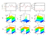
Figure 1: Real and imaginary parts of complex potential (11) and (12) are shown by the black solid and red dashed curves, respectively, for (a) $W(x)=\exp(-B_{1}x^{2})$, (b) $W(x)=x\exp(-B_{2}x^{2})$, and (c) $W(x)=V_{0}/2+V_{1}\cos(qx)$. (d-f): Evolution of truncated CA solutions which are not supported by the correct phase structure, in the presence of the potentials corresponding to (a-c). (g-i): The evolution of the truncated solutions with the correct phase structure in the same cases (a-c). Here we set $A=0.5$ and $\beta=1$, the other parameters being $B_{1}=1$ in (a); $B_{2}=0.5$ in (b); $V_{0}=4$, $V_{1}=0.2$ and $q=1$ in (c); $B_{1}=1$ and $g=-1$ in (d) and (g); $B_{2}=0.5$ and $g=-1$ in (e) and (h); and $V_{0}=4$, $V_{1}=0.2$, $q=1$ and $g=1$ in (f) and (i).

To exhibit properties of such CA solutions, we consider three complex potentials which are relevant for various physical realizations, viz., ones generated by $W(x)=\exp(-B_{1}x^{2})$, $W(x)=x\exp(-B_{2}x^{2})$, and

$$W(x)=\frac{1}{2}V_{0}+V_{1}\cos(qx).$$ (13)

The first and last potentials are $\mathcal{PT}$-symmetric, while the second one is not, as shown in Figs. 1(a)-1(c).

To illustrate the dynamics of CA states under the action of these potentials, we have simulated the evolution of such states in a spatially truncated form. When the initial state is not given the correct phase structure, determined by solution (10), but is simply taken in a real form, $\Psi(x,0)\equiv A$, the light diffracts fast to the gain region, as seen in Figs. 1(d)-1(f). On the other hand, for the truncated solution carrying the correct phase distribution, the diffraction is strongly suppressed, as shown in Figs. 1(g)-1(i). We also find that, naturally, the larger the truncation width is at $z=0$, the longer the diffraction-free propagation distance is (not shown here in detail). In the rest of the paper, we focus on CA states supported by the periodic complex potential (13), which is most relevant for the realization by means of photonic lattices in optical media.

3 Modulational instability of the constant-amplitude (CA) solutions

In this section, we address the stability of the CA solutions by employing the linear-stability analysis, based on the plane-wave-expansion method, and direct numerical simulations. We note that, although the familiar linear-stability analysis, previously elaborated for models with localized potentials $V(x)$ BOOK_YJK , can be readily applied to Eq. (1), it cannot be used to obtain the stability band structure in the presence of the periodic potential. Here, we apply the plane-wave-expansion method NatureCommunication6_7257 to study the stability of the CA solution (10) in the latter case. As an example of the periodic potential, we choose the $\mathcal{PT}$-symmetric one, which is displayed in Fig. 1(c) and generated by Eqs. (11) and (12) with $W(x)=V_{0}/2+V_{1}\cos(qx)$:

$$V_{R}\left(x\right) =-\frac{\beta V_{1}q^{2}}{6}\cos\left(qx\right)+\frac{1}{2}\left[\frac{V_{0}}{2}+V_{1}\cos\left(qx\right)\right]^{2}$$

$$-\frac{\beta}{6}\left[\frac{V_{0}}{2}+V_{1}\cos\left(qx\right)\right]^{3},$$ (14)

$$V_{I}\left(x\right) =\frac{qV_{1}}{2}\left[1-\beta\left(\frac{V_{0}}{2}+V_{1}\cos\left(qx\right)\right)\right]\sin\left(qx\right),$$ (15)

the corresponding CA solution (10) being

$$\Psi\left(x,z\right)=A\exp\left[i\Xi\left(x,z\right)\right],$$ (16)

where $\Xi\left(x,z\right)=gA^{2}z+V_{0}x/2+(V_{1}/q)\sin(qx)$.

The linear-stability analysis can be performed by adding small perturbations to the CA solution (16):

$$\Psi\left(x,z\right)=\left[A+\varepsilon F_{\lambda}\left(x\right)e^{i\lambda z}+\varepsilon G_{\lambda}^{\ast}\left(x\right)e^{-i\lambda^{\ast}z}\right]e^{i\Xi\left(x,z\right)},$$ (17)

where the asterisk stands for the complex conjugation and $\varepsilon$ is a real infinitesimal amplitude of the perturbation with complex eigenfunctions $F_{\lambda}\left(x\right)$ and $G_{\lambda}\left(x\right)$, that are associated to a complex eigenvalue, $\lambda$. As usual, the imaginary part of $\lambda$ measures the instability growth rate of the perturbation, and thus determines whether the CA solution is stable. The substitution of expression (17) in Eq. (1) and linearization leads to the eigenvalue problem in the matrix form

$$\left(\begin{array}[c]{cc}L_{1}&gA^{2}\\ -gA^{2}&L_{2}\end{array}\right)\left(\begin{array}[c]{c}F_{\lambda}\left(x\right)\\ G_{\lambda}\left(x\right)\end{array}\right)=\lambda\left(\begin{array}[c]{c}F_{\lambda}\left(x\right)\\ G_{\lambda}\left(x\right)\end{array}\right),$$ (18)

where the operators $L_{1}$ and $L_{2}$ are

$$L_{1} = gA^{2}+\frac{1}{2}\partial_{xx}+i\frac{\beta}{6}\partial_{xxx}+iW\partial_{x}$$ (19)

$$-\frac{\beta}{2}W_{x}\partial_{x}-\frac{\beta}{2}W\partial_{xx}-i\frac{\beta}{2}W^{2}\partial_{x},$$

$$L_{2} = -gA^{2}-\frac{1}{2}\partial_{xx}+i\frac{\beta}{6}\partial_{xxx}+iW\partial_{x}$$ (20)

$$+\frac{\beta}{2}W_{x}\partial_{x}+\frac{\beta}{2}W\partial_{xx}-i\frac{\beta}{2}W^{2}\partial_{x}.$$

As said above, we apply the plane-wave-expansion method NatureCommunication6_7257 to study the MI of the CA solution (16) in the periodic $\mathcal{PT}$-symmetric potential $V(x)$ given by Eqs. (14) and (15). In the framework of the method, when $W(x)$ is a periodic function with period $2\pi/q$, perturbation eigenmodes $F_{\lambda}\left(x\right)$ and $G_{\lambda}\left(x\right)$, along with $W(x)$ itself, can be expanded into Fourier series, according to the Floquet-Bloch theorem:

$$\left(\begin{array}[c]{c}F_{\lambda}\left(x\right)\\ G_{\lambda}\left(x\right)\end{array}\right) ={\displaystyle\sum_{n=-\infty}^{+\infty}}\left(\begin{array}[c]{c}u_{n}(k)\\ v_{n}(k)\end{array}\right)e^{i(qn+k)x},$$ (25)

$$W(x) ={\displaystyle\sum_{n=-\infty}^{+\infty}}W_{n}e^{iqnx},$$ (26)

where $k$ is the Bloch momentum, the presence of which makes the eigenmodes quasiperiodic. Substituting Eqs. (14), (15), (25) and (26) into the eigenvalue problem (18), one arrives at the following system of linear equations for perturbation amplitudes $u_{n}$, $v_{n}$ and eigenvalue $\lambda(k)$:

$$\lambda u_{n} =gA^{2}v_{n}+\alpha_{n}u_{n}+\beta_{n-1}u_{n-1}$$

$$+\gamma_{n+1}u_{n+1}+\theta_{n-2}u_{n-2}+\theta_{n+2}u_{n+2},$$ (27)

$$\lambda v_{n} =-gA^{2}u_{n}+\sigma_{n}v_{n}+\delta_{n-1}v_{n-1}$$

$$+\eta_{n+1}v_{n+1}+\theta_{n-2}v_{n-2}+\theta_{n+2}v_{n+2},$$ (28)

where we define

$$\alpha_{n} =gA^{2}-\frac{V_{0}}{8}\left(4-\beta V_{0}\right)\left(qn+k\right)$$

$$-\frac{1}{4}\left(2-\beta V_{0}\right)\left(qn+k\right)^{2}+\frac{\beta}{6}\left(qn+k\right)^{3},$$

$$\beta_{n} =-\frac{V_{1}}{4}\left(2-\beta q\right)\left(qn+k\right)+\frac{\beta V_{1}}{4}\left(qn+k\right)^{2},$$

$$\gamma_{n} =-\frac{V_{1}}{4}\left(2+\beta q\right)\left(qn+k\right)+\frac{\beta V_{1}}{4}\left(qn+k\right)^{2},$$

$$\theta_{n} =\frac{\beta V_{1}^{2}}{8}\left(qn+k\right),$$

$$\sigma_{n} =-gA^{2}-\frac{1}{8}V_{0}\left(4-\beta V_{0}\right)\left(qn+k\right)$$

$$+\frac{1}{4}\left(2-\beta V_{0}\right)\left(qn+k\right)^{2}+\frac{\beta}{6}\left(qn+k\right)^{3},$$

$$\delta_{n} =-\frac{V_{1}}{4}\left(2+\beta q\right)\left(qn+k\right)-\frac{\beta V_{1}}{4}\left(qn+k\right)^{2},$$

$$\eta_{n} =-\frac{V_{1}}{4}\left(2-\beta q\right)\left(qn+k\right)-\frac{\beta V_{1}}{4}\left(qn+k\right)^{2}.$$

In the absence of the TOD ($\beta=0$) the results for the MI, i.e., eigenvalues $\lambda(k)$, produced by the present analysis, are consistent with those reported in Ref. NatureCommunication6_7257 . In the following, the growth rate of the MI of the CA solution is defined as the largest imaginary part of $\lambda(k)$. As a typical example, Fig. 2 depicts the dependence of $\max[\operatorname{Im}\{\lambda\}]$ on $k$ (in the half of the first Brillouin zone) for the different TOD strengths (of either sign) in both the self-focusing and defocusing regimes.

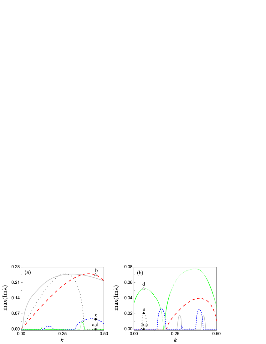
Figure 2: The dependence of the MI growth rate, i.e., the largest imaginary part of eigenvalues $\lambda(k)$, on the Bloch wavenumber $k$ (in the half of the first Brillouin zone) for different values of the TOD coefficient, in the system containing periodic potential (13). Panels (a) and (b) report the results, severally, for the self-focusing ($g=1$) and defocusing ($g=-1$) nonlinearity, with the black dotted, red dashed, gray solid, blue short-dashed, and green short-dotted curves corresponding, respectively, to $\beta=-3$, $-1$, $0$, $1$, and $3$ in (a), and $\beta=-3$, $-1$, $0$, $0.2$, and $0.45$ in (b); note the difference in the scales of vertical axes in panels (a) and (b). Here the amplitude of the unperturbed solution is $A=0.5$, and the other parameters are $V_{0}=4$, $V_{1}=0.2$, and $q=1$.

For the self-focusing nonlinearity [Fig. 2(a)], at $\beta=0$, as well as at a close value, $\beta=-1$, the MI eigenvalues with the largest imaginary part are complex at all $k$ [see the gray solid and red dashed curves in Fig. 2(a)], hence the CA waves are linearly unstable to all perturbations, as shown in Ref. NatureCommunication6_7257 for $\beta=0$. The situation changes in the presence of sufficiently strong TOD. As shown by the black dotted curve pertaining to $\beta=-3$ in Fig. 2(a), the CA solution is stable against perturbations corresponding to the Floquet-Bloch modes close to the edge of the Brillouin zone. The positive TOD, with $\beta>0$, strongly suppresses the instability [see the blue and green short-dashed lines in Fig. 2(a), corresponding to $\beta=+1$ and $+3$, respectively]. Thus, the TOD terms provides for partial stabilization of the CA waves, under the action of the self-focusing nonlinearity. This finding may be qualitative understood as a manifestation of the trend, imposed by the TOD, to replace the strong absolute instability by its weaker convective counterpart.

The situation is different for the defocusing nonlinearity [Fig. 2(b)]. At $\beta=0$, there are narrow MI bands NatureCommunication6_7257 , shown by the gray solid curve in Fig. 2(b). Indeed, it is natural that the self-defocusing gives rise to weaker MI, if any. The TOD with $\beta<0$ originally enhances the MI [see the red dashed curve in Fig. 2(b) corresponding to $\beta=-1$], which is followed by the suppression of the MI at larger values of $-\beta$, as shown by the black dotted curve corresponding to $\beta=-3$. The MI is completely absent at $\beta<-3$, as can be seen below in Fig. 6(b). On the other hand, the increase of $\beta>0$ leads to strong amplification of the MI; in particular, the green short-dotted curve in Fig. 2(b), corresponding to a relatively small positive TOD coefficient, $\beta=0.45$, demonstrates strong instability to the perturbation with all values of $k$.

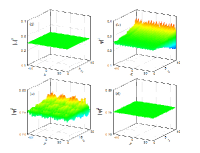
Figure 3: Numerically simulated evolution of an unstable CA wave under the action of the self-focusing nonlinearity ($g=1$) and periodic complex potential (13). (a) $\beta=-3;$ (b) $\beta=-1$; (c) $\beta=1$, and (d) $\beta=3$. Here, we fix the perturbation parameters as $\varepsilon=0.01$ and $k=0.45$, the other parameters being the same as in Fig. 2.

To explore the nonlinear development of the MI, we have performed systematic simulations of Eq. (1), taking inputs in the form of unstable CA solutions with the addition of small perturbations corresponding to specific Floquet-Bloch eigenmodes, as per Eq. (17). The results are summarized in Figs. 3 and 4, for the amplitude of the unperturbed solution $A=0.5$, and the perturbation amplitude $\varepsilon=0.01$.

Figure 3 shows the evolution of the CA solution perturbed by the eigenmodes at $k=0.45$ for different values of the TOD coefficient, $\beta$, in the self-focusing regime. The so built solution is stable for $\beta=-3$ and $+3$ [Figs. 3(a,d)], and unstable for $\beta=-1$ and $+1$ [Figs. 3(b,c)]. These findings are consistent with results of the linear-stability analysis, which predicts no instability for $k=0.45$ and $\beta=\mp 3$, as shown by the points “a” and “d” in Fig. 2(a) [although points “a” and “d” seem identical in Fig. 2(a), they correspond to the different values of the TOD coefficient], while for $\beta=-1$ and $+1$ the instability growth rates, i.e., $\max[\operatorname{Im}\{\lambda\}]$, are $0.24428$ and $0.04544$, respectively, see the points “b” and “c” in Fig. 2(a).

Figure 4(a) shows that, at negative $\beta$, the unstable CA wave is split by the MI into a chain of soliton, which is the same outcome as in the case of the usual self-focusing NLS equation with $\beta=0$, cf. Fig. 4(b). At $\beta>0$, the MI cannot form a chain of solitons because the initial perturbation eigenmode is not a simple periodic wave like sine or cosine, see Fig. 4(c).

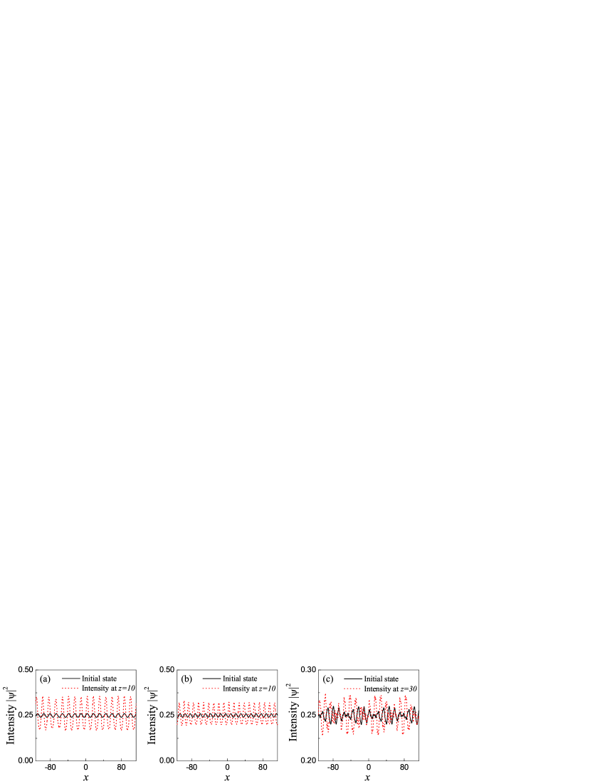
Figure 4: The distributions of the initial intensity and the intensity at the distance $z$, as produced by numerical simulations. (a) $\beta=-1$ and $z=10$; (b) $\beta=0$ and $z=10$, and (c) $\beta=1$ and $z=30$. Parameters are the same as in Fig. 3.

Figure 5 displays the simulated evolution in the system with the defocusing nonlinearity, where the perturbation eigenmodes with $k=0.06$ are initially added. This figure demonstrates, in agreement with the prediction of the linear-stability analysis summarized in Fig. 2(b), that the CA wave is stable to these perturbations at $\beta=-1$ and $+0.2$, see Figs. 5(b) and 5(c) and the corresponding points “b” and “c” in Fig. 2(b) [points “b” and “c”, which seem identical in Fig. 2(b), correspond to different values of the TOD coefficient]. On the other hand, the solution is unstable at $\beta=0.45$, see Fig. 5(d) and the corresponding point “d” in Fig. 2(b). A specific situation is observed at $\beta=-3$. While the linear-stability analysis predicts the MI in this case [see the point “a” in Fig. 2(b)], direct simulations reveal some fluctuations, but no exponentially growing instability, as shown in Fig. 5(a). This happens because the corresponding growth rate is very small, $\max[\operatorname{Im}\{\lambda\}]\approx$ $0.02049$. The result shows an example of weak stability observed at very small MI growth rates.

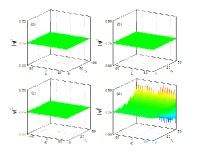
Figure 5: The same as in Fig. 3, but for the defocusing nonlinearity ($g=-1$), $\varepsilon=0.01$, and $k=0.06$. (a) $\beta=-3$; (b) $\beta=-1$; (c) $\beta=0.2$, and (d) $\beta=0.45$.

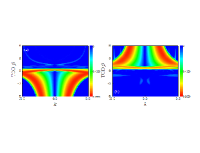
Figure 6: The dependence of the largest imaginary part of the MI eigenvalues on the TOD strength, $\beta$, in the first Brillouin zone of periodic potential (13) for (a) $g=1$ and (b) $g=-1$ (self-focusing and defocusing, respectively), while the other parameters are the same as in Fig. 2.

To display the effect of the TOD on the MI of the CA waves, Fig. 6 depicts the dependence of the largest imaginary part of the MI eigenvalues on the TOD coefficient, $\beta$, in the first Brillouin zone for the self-focusing and defocusing nonlinearities. For the self-focusing case, Fig. 6(a) shows that the MI takes place (with complex most unstable eigenvalues) for all $k$ when $\beta$ belongs to interval $-1.6<\beta<0.66$. However, at $\beta<-1.6$, a stability band emerges at the edge of the Brillouin zone, whose size grows with the increase of $|\beta|$, while as $\beta>0.66$, the stability band is quite broad, while the remaining instability is weak.

Figure 6(b) shows an opposite situation in the case of the defocusing nonlinearity. The difference is explained by the fact that, at $\beta=0$, a stability band does not exist for the self-focusing nonlinearity, but it is present in the defocusing case, as can be seen in Fig. 2(b). Despite the difference, a general conclusion is that the TOD effect eventually tends to attenuate the MI of the CA waves.

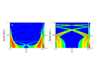
Figure 7: The dependence of the MI growth rate, on the amplitude, $A$, and wavenumber, $k$, of the CA solution, supported by the complex periodic potential (13). (a) $g=1$, $\beta=1$; (b) $g=-1$, $\beta=-1$, the other parameters being $V_{0}=4$, $V_{1}=0.2$, and $q=1$.

The above analysis was reported for the MI of the CA solution with $A=0.5$. Now, we aim to consider the effect of the variation of the amplitude on the MI. Figure 7 presents the dependence of the MI growth rate on $A$ in the first Brillouin zone for the self-focusing and defocusing nonlinearities, respectively. Fig. 7(a) demonstrates that, for the self-focusing nonlinearity, the instability bands are mainly concentrated at the edge of the first Brillouin zone for $\beta=1$, shrinking with the increase of $A$ until reaching $A\approx 2$, where the MI virtually disappears. For the defocusing nonlinearity, Fig. 7(b) demonstrates that the stability band is mainly focused at the center of the first Brillouin zone. Its size grows with the increase of $A$ up to $A\approx 1.1$, at $\beta=-1$. With the further increasing of $A$, the instability bands start to converge and cross until vanishing at $A\approx 2.3$.

Lastly, it is relevant to address the stability of the zero state in the model based on Eq. (1), which corresponds to amplitude $A=0$ of the unperturbed CA state. Usually, the stability of the zero background is an important issue in the analysis of $\mathcal{PT}$-symmetric systems Rep.Prog.Phys70_947 ; PRL80_5243 ; JMP43_2814 ; PRL89_270401 . From Fig. 8, one can conclude that the stability bands of the zero state are mainly concentrated at the center of the first Brillouin zone for both the self-focusing and defocusing nonlinearity, as shown in Fig. 8(a), in which, at $g=1$, the stability band of the zero solution is $|k|\leq 0.06$ for $\beta=1$, while at $g=-1$ it is $|k|\leq 0.18$ for $\beta=-1$. In this case, the dependence of the instability growth rate of the zero solution on the TOD strength $\beta$ and wavenumber $k$ is shown in Fig. 8(b). From here, one can see that the zero state is stable for all $k$ when $\beta$ belongs to intervals $\beta\leq-3.3$, or $-0.8<\beta<0.6$, or $\beta>2$. At $-1.5<\beta<-3.3$, the instability band is mainly concentrated near the center of the first Brillouin zone, while, at $-1.5<\beta<-0.8$, the instability is concentrated at the edge of the first Brillouin zone. For $0.6<\beta<2$, instability bandgaps form at some values of $k$.

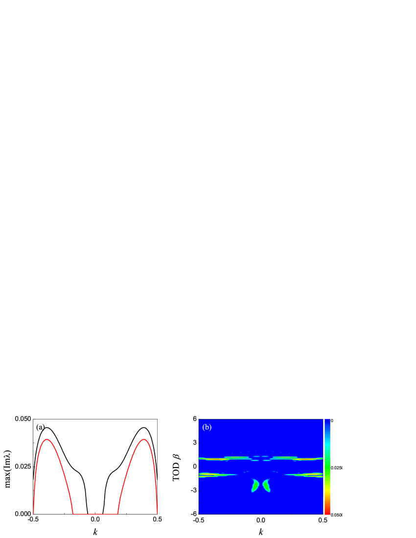
Figure 8: (a) The dependence of the largest imaginary part of eigenvalues on the Bloch wavenumber $k$ for the zero state, which corresponds to the zero amplitude of the underlying CA solution, $A=0$. Here, the black solid and red solid curves represent $g=1$, $\beta=1$ and $g=-1$, $\beta=-1$, respectively. (b) The dependence of the MI growth rate on the TOD strength $\beta$ and wavenumber $k$ for the self-focusing nonlinearity ($g=1$). The other parameters are the same as in Fig. 7.

4 Conclusion

We have considered the CA (constant-amplitude) waves governed by the NLS equation which includes the spatial TOD (third-order dispersion) and complex potentials (thus corresponding to a non-Hermitian Hamiltonian). The model was built as a solution of the inverse problem, which predicts the complex potential needed to support a CA state with a required phase-gradient structure. The setting can be realized in optical nonlinear waveguides, with an appropriate distribution of the local gain and loss. The results show, first, that the diffraction of the truncated CA solution is strongly suppressed, if the state carries the correct phase structure. The main part of the analysis was focused on the MI (modulation instability) of the CA waves, by means of the linear-stability analysis based on the plane-wave expansion method, and with the help of direct numerical simulations. The results have shown that the TOD tends to attenuate the MI. This may be understood as a manifestation of the trend, imposed by the TOD, to transform strong absolute instability into a weaker convective form. Direct simulations of the perturbed evolution of the CA waves have revealed a phenomenon of the weak stability, which occurs at sufficiently small values of the MI instability growth rate, when formally unstable CAs turn out to be effectively stable, in terms of the simulated evolution. The approach elaborated in the present work can be used to analyze the stability band structure of periodic solutions in periodic complex potentials for other wave systems.

References

- (1) C. M. Bender, Rep. Prog. Phys. 70, 947 (2007).
- (2) C. M. Bender and S. Boettcher, Phys. Rev. Lett. 80, 5243 (1998).
- (3) A. Mostafazadeh, J. Math. Phys. 43, 205 (2002).
- (4) C. M. Bender, D. C. Brody, and H. F. Jones, Phys. Rev. Lett. 89, 270401 (2002).
- (5) A. Guo, G. J. Salamo, D. Duchesne, R. Morandotti, M. Volatier-Ravat, V. Aimez, G. A. Siviloglou, and D. N. Christodoulides, Phys. Rev. Lett. 103, 093902 (2009).
- (6) C. E. Rüter, K. G. Makris, R. El-Ganainy, D. N. Christodoulides, M. Segev, and D. Kip, Nat. Phys. 6, 192 (2010); T. Kottos, ibid. 6, 166 (2010).
- (7) A. Regensburger, C. Bersch, M. -A. Miri, G. Onishchukov, D. N. Christodoulides, and U. Peschel, Nature (London)488, 167 (2012).
- (8) L. Feng, Y. -L. Xu, W. S. Fegadolli, M. -H. Lu, J. E. B. Oliveira, V. R. Almeida, Y. -F. Chen, and A. Scherer, Nat. Mater. 12, 108 (2013).
- (9) B. Peng, S. Kayaözdemir, F. Lei, F. Monifi, M. Gianfreda, G. L. Long, S. Fan, F. Nori, C. M. Bender, and L. Yang, Nat. Phys. 10, 394 (2014).
- (10) K. G. Makris, R. El-Ganainy, D. N. Christodoulides, and Z. H. Musslimani, Phys. Rev. Lett. 100, 103904 (2008).
- (11) A. Guo, G. J. Salamo, D. Duchesne, R. Morandotti, M. Volatier-Ravat, V. Aimez, G. A. Siviloglou, and D. N. Christodoulides, Phys. Rev. Lett. 103, 093902 (2009).
- (12) H. Ramezani, T. Kottos, R. El-Ganainy, and D. N. Christodoulides, Phys. Rev. A 82, 043803 (2010).
- (13) Z. Lin, H. Ramezani, T. Eichelkraut, T. Kottos, H. Cao, and D. N. Christodoulides, Phys. Rev. Lett. 106, 213901 (2011).
- (14) N. Bender, S. Factor, J. D. Bodyfelt, H. Ramezani, D. N. Christodoulides, F. M. Ellis, and T. Kottos, Phys. Rev. Lett. 110, 234101 (2013).
- (15) Y. Sun, W. Tan, H. Q. Li, J. Li, and H. Chen, Phys. Rev. Lett. 112, 143903 (2014).
- (16) L. Feng, Z. J. Wong, R. -M. Ma, Y. Wang, and X. Zhang, Science 346, 972 (2014).
- (17) H. Hodaei, M. -A. Miri, M. Heinrich, D. N. Christodoulides, and M. Khajavikhan, Science 346, 975 (2014).
- (18) Z. H. Musslimani, K. G. Makris, R. El-Ganainy, and D. N. Christodoulides, Phys. Rev. Lett. 100, 030402 (2008).
- (19) F. Kh. Abdullaev, Y. V. Kartashov, V. V. Konotop, and D. A. Zezyulin, Phys. Rev. A 83, 041805(R) (2011).
- (20) X. Zhu, H. Wang, L. X. Zheng, H. G. Li, and Y. J. He, Opt. Lett. 36, 2680 (2011).
- (21) H. G. Li, Z. W. Shi, X. J. Jiang, and X. Zhu, Opt. Lett.36, 3290 (2011).
- (22) S. Hu, X. Ma, D. Lu, Z. Yang, Y. Zheng, and W. Hu, Phys. Rev. A 84, 043818 (2011).
- (23) S. Nixon, L. Ge, and J. Yang, Phys. Rev. A 85, 023822 (2012).
- (24) D. A. Zezyulin and V. V. Konotop, Phys. Rev. A 85, 043840 (2012).
- (25) V. Achilleos, P. G. Kevrekidis, D. J. Frantzeskakis, and R. Carretero-González, Phys. Rev. A 86, 013808 (2012).
- (26) M. -A. Miri, A. B. Aceves, T. Kottos, V. Kovanis, and D. N. Christodoulides, Phys. Rev. A 86, 033801 (2012).
- (27) B. Midya and R. Roychoudhury, Phys. Rev. A 87, 045803 (2013).
- (28) C. P. Jisha, L. Devassy, A. Alberucci, and V. C. Kuriakose, Phys. Rev. A 90, 043855 (2014).
- (29) N. Lazarides and G. P. Tsironis, Phys. Rev. Lett.110, 053901 (2013).
- (30) G. Castaldi, S. Savoia, V. Galdi, A. Alù, and N. Engheta, Phys. Rev. Lett. 110, 173901 (2013).
- (31) A. Lupu, H. Benisty, and A. Degiron, Opt. Express 21, 21651 (2013).
- (32) L. Feng, M. Ayache, J. Huang, Y. -L. Xu, M. -H. Lu, Y. -F. Chen, Y. Fainman, and A. Scherer, Science 333, 729 (2011).
- (33) V. V. Konotop, J. Yang, and D. A. Zezyulin, Rev. Mod. Phys. 88, 035002 (2016).
- (34) S. M. Hu and W. Hu, Eur. Phys. J. D 66, 266 (2012).
- (35) H. Wang, S. Shi, W. He, X. Zhu, and Y. He, Eur. Phys. J. D 68, 322 (2014).
- (36) H. Wang, D. Ling, G. Chen, X. Zhu, and Y. He, Eur. Phys. J. D 69, 31 (2015).
- (37) X. Zhu, and H. Li, Eur. Phys. J. D 70, 14 (2016).
- (38) K. A. Muhsina, and P. A. Subha, Eur. Phys. J. D 69, 171 (2015).
- (39) B. Liu, L. Li, and D. Mihalache, Rom. Rep. Phys. 67, 802 (2015).
- (40) P. F. Li, B. Li, L. Li, and D. Mihalache, Rom. J. Phys. 61, 577 (2016).
- (41) P. F. Li, D. Mihalache, and L. Li, Rom. J. Phys. 61, 1028 (2016).
- (42) H. Cartarius and G. Wunner, Phys. Rev. A 86, 013612 (2012).
- (43) F. Single, H. Cartarius, G. Wunner, and J. Main, Phys. Rev. A 90, 042123 (2014).
- (44) D. Dast, D Haag, H. Cartarius, and G. Wunner, Phys. Rev. A 93, 033617 (2016).
- (45) C. Hang, D. A. Zezyulin, V. V. Konotop, and G. Huang, Opt. Lett. 38, 4033 (2013).
- (46) C. Hang, D. A. Zezyulin, G. Huang, V. V. Konotop, and B. A. Malomed, Opt. Lett. 39, 5387 (2014).
- (47) H. Zhong, B. Zhu, X. Qin, J. Huang, Y. Ke, Zh. Zhou, and C. Lee, Eur. Phys. J. D 70, 157 (2016).
- (48) H. Sakaguchi and B. A. Malomed, Phys. Rev. E 77, 056606 (2008).
- (49) S. Nixon and J. Yang, Opt. Lett. 41, 2747 (2016).
- (50) S. Nixon and J. Yang, Physica D 331, 48 (2016).
- (51) J. Yang and S. Nixon, Phys. Lett. A 380, 3803 (2016) .
- (52) Y. D. Chong, L. Ge, H. Cao, and A. D. Stone, Phys. Rev. Lett. 105, 053901 (2010).
- (53) W. Wan, Y. Chong, L. Ge, H. Noh, A. D. Stone, and H. Cao, Science 331, 889 (2011).
- (54) M. Liertzer, L. Ge, A. Cerjan, A. D. Stone, H. E. Türeci, and S. Rotter, Phys. Rev. Lett. 108, 173901 (2012).
- (55) M. Brandstetter, M. Liertzer, C. Deutsch, P. Klang, J. Schöberl, H. E. Türeci, G. Strasser, K. Unterrainer, and S. Rotter, Nat. Commun 5, 4034 (2014).
- (56) B. Peng, S. K. Özdemir, S. Rotter, H. Yilmaz, M. Liertzer, F. Monifi, C. M. Bender, F. Nori, L. Yang, Science 346, 328 (2014).
- (57) T. B. Benjamin and J. E. Feir, J. Fluid Mech. 27, 417 (1967).
- (58) T. Taniuti and H. Washimi, Phys. Rev. Lett. 21, 209 (1968).
- (59) S. Ghosha and M. P. Rishi, Eur. Phys. J. D 19, 223 (2002).
- (60) N. Nimje, S. Dubey, and S. K. Ghosh, Eur. Phys. J. D 59, 223 (2010).
- (61) C. B. Tabi, A. Mohamadou, and T. C. Kofane, Eur. Phys. J. B 74, 151 (2010).
- (62) G. Sharma and S. Ghosh, Eur. Phys. J. D 11, 301 (2000).
- (63) K. Tai, A. Hasegawa, and A. Tomita, Phys. Rev. Lett. 56, 135 (1986).
- (64) G. P. Agrawal, Nonlinear Fiber Optics (Academic Press, San Diego: 1995).
- (65) J. Meier, G. I. Stegeman, D. N. Christodoulides, Y. Silberberg, R. Morandotti, H. Yang, G. Salamo, M. Sorel, and J. S. Aitchison, Phys. Rev. Lett. 92, 163902 (2004).
- (66) M. Onorato, A. R. Osborne, and M. Serio, Phys. Rev. Lett. 96, 014503 (2006).
- (67) J. T. Cole and Z. H. Musslimani, Physica D 313, 26 (2015).
- (68) I. Kourakis and P. K. Shukla, Eur. Phys. J. B 50, 321 (2006).
- (69) M. M. de. Castro, D. Gomila, and R. Zambrini, Eur. Phys. J. Special Topics 203, 217 (2012).
- (70) R. S. Tasgal and B. A. Malomed, Phys. Scripta 60, 418 (1999).
- (71) I. A. Bhat, T. Mithun, B. A. Malomed, and K. Porsezian, Phys. Rev. A 92, 063606 (2015).
- (72) K. Li and P. G. Kevrekidis, Phys. Rev. E 83, 066608 (2011).
- (73) R. Driben and B. A. Malomed, Opt. Lett. 36, 4323 (2011).
- (74) Y. V. Bludov, R. Driben, V. V. Konotop, and B. A. Malomed, J. Opt. 15, 064010 (2013).
- (75) X. Ren, H. Wang, H. Wang, and Y. He, Opt. Express 22, 19774 (2014).
- (76) L. Ge, M. Shen, T. Zang, C. Ma, and L. Dai, Phys. Rev. E 91, 023203 (2015).
- (77) Z. Yan, Z. Wen, and C. Hang, Phys. Rev. E 92, 022913 (2015).
- (78) K. G. Makris, Z. H. Musslimani, D. N. Christodoulides, and S. Rotter, Nat. Commun. 6, 7257 (2015).
- (79) M. Notomi, Rep. Prog. Phys. 73, 096501 (2010).
- (80) Y. Chen and Z. Y. Yan, Scientific Reports 6, 23478 (2016).
- (81) J. R. Marciante and G. P. Agrawal, IEEE J. Quant. Electr. 32, 590 (1996).
- (82) L. D. Carr, C. W. Clark, and W. P. Reinhardt, Phys. Rev. A 62, 063610 (2000); J. C. Bronski, L. D. Carr, B. Deconinck, J. N. Kutz, and K. Promislow, Phys. Rev. E 63, 036612 (2001); J. C. Bronski, L. D. Carr, R. Carretero-González, B. Deconinck, J. N. Kutz, and K. Promislow, Phys. Rev. E 64, 056615 (2001); J. Belmonte-Beitia, V. V. Konotop, V. M. Pérez-García, and V. E. Vekslerchik, Chaos, Solitons Fractals 41, 1158 (2009); B. A. Malomed and Yu. A. Stepanyants, Chaos 20, 013130 (2010).
- (83) I. V. Barashenkov, D. A. Zezyulin and V. V. Konotop, Non-Hermitial Hamiltonians in Quantum Physics, Springer International Publishing, Switzerland, 2016, pp.143-155.
- (84) D. A. Zezyulin, I. V. Barashenkov, and V. V. Konotop, Phys. Rev. A 94, 063649 (2016).
- (85) J. Yang, Nonlinear Waves in Integrable and Nonintegrable Systems (SIAM, Philadelphia, 2010).