H₂CO distribution and formation in the TW Hya disk

Abstract

H₂CO is one of the most readily detected organic molecules in protoplanetary disks. Yet its distribution and dominant formation pathway(s) remain largely unconstrained. To address these issues, we present ALMA observations of two H₂CO lines ($3_{12}-2_{11}$ and $5_{15}-4_{14}$) at 0$\farcs$5 ($\sim$30 au) spatial resolution toward the disk around the nearby T Tauri star TW Hya. Emission from both lines is spatially resolved, showing a central depression, a peak at $0\farcs 4$ radius, and a radial decline at larger radii with a bump at $\sim 1^{\prime\prime}$, near the millimeter continuum edge. We adopt a physical model for the disk and use toy models to explore the radial and vertical H₂CO abundance structure. We find that the observed emission implies the presence of at least two distinct H₂CO gas reservoirs: (1) a warm and unresolved inner component ($<10$ au), and (2) an outer component that extends from $\sim 15$ au to beyond the millimeter continuum edge. The outer component is further constrained by the line ratio to arise in a more elevated disk layer at larger radii. The inferred H₂CO abundance structure agrees well with disk chemistry models, which predict efficient H₂CO gas-phase formation close to the star, and cold H₂CO grain surface formation, through H additions to condensed CO, followed by non-thermal desorption in the outer disk. The implied presence of active grain surface chemistry in the TW Hya disk is consistent with the recent detection of CH₃OH emission, and suggests that more complex organic molecules are formed in disks, as well.

1. Introduction

Planets are assembled and obtain their initial organic compositions from solids and gas in protoplanetary disks. Terrestrial, rocky planets are expected to form close to their stars and directly sample the inner disk refractory organics, though some volatile organics could be added through direct accretion of disk gas. More volatile organic material from the outer disk can become incorporated into the planet by later planetesimal bombardment (Morbidelli et al., 2012; Raymond et al., 2014). The abundance of volatile organics on nascent planets are of particular interest, since they can drive a complex prebiotic chemistry leading to formation of the different building blocks of RNA and proteins (Powner et al., 2009).

Based on cometary studies, volatile organics were common in the Solar Nebula; comets frequently contain anywhere between a few and 10% of volatile organics with respect to water ice (Mumma & Charnley, 2011; Le Roy et al., 2015). The most abundant ones are CH₃OH, CH₄, C₂H₂, H₂CO, C₂H₆ and HCN. Of these, CH₃OH, C₂H₂, H₂CO and HCN have also been detected in gas form in protoplanetary disks, suggesting that, similar to the Solar System planets, exoplanets form in environments rich in volatile organic species (e.g. Dutrey et al., 1997; Aikawa et al., 2003; Carr & Najita, 2008; Walsh et al., 2016).

Of these molecules, H₂CO and CH₃OH are of special prebiotic interest. Both can form through grain surface hydrogenation of condensed CO and become incorporated into icy bodies. Based on laboratory experiments, such organic-rich ices become sources of a range of complex organic molecules when exposed to any kind of high-energy radiation or electrons (e.g. Gerakines et al., 1996; Hudson & Moore, 2000; Bennett et al., 2007; Öberg et al., 2009; Öberg, 2016; Boyer et al., 2016; Sullivan et al., 2016). CH₃OH only forms through ice chemistry, and if it was readily observable it would be the best tracer of organic ice chemistry in disks. CH₃OH is challenging to detect, however, due to its low volatility and large partition function. To date it has only been observed in a single disk at low SNR, resulting in very limited constraints on its radial or vertical distribution (Walsh et al., 2016).

H₂CO is easier to observe (Aikawa et al., 2003; Öberg et al., 2010, 2011; van der Marel et al., 2014), but connecting these observations to disk ice chemistry is complicated by its viable gas-phase formation pathways. High spatial resolution observations are needed to decide between gas and grain surface formation pathways. H₂CO grain surface formation would only be expected where it is cold enough for CO to accrete onto grains and remain there for a sufficient time to allow chemical reactions with H (Watanabe & Kouchi, 2002; Fuchs et al., 2009; Cuppen et al., 2009). In a disk with a radially decreasing temperature profile, H₂CO formed through such grain surface chemistry should only appear at a distance from the central star corresponding to midplane temperatures below 20–30 K (Fayolle et al., 2016). Though possible everywhere in the disk, gas-phase H₂CO formation is expected to occur most efficiently in the warm and dense inner disk, producing a centrally peaked H₂CO abundance and emission profile.

H₂CO has been observed at high spatial resolution with ALMA in one disk, around DM Tau; where Loomis et al. (2015) found that H₂CO is distributed throughout the disk, i.e a hybrid of what is expected from pure gas-phase or grain-surface chemistry. This result was used to conclude that H₂CO forms through both gas and grain surface chemistry in this disk, since neither pathway can explain all the observed emission.

In this study, we revisit the distribution and chemistry of H₂CO in disks by characterizing its abundance pattern in an older example, the disk around TW Hya. Because TW Hya is nearby (d=59 pc (Gaia Collaboration et al., 2016)), analogous observations provide access to smaller physical scales compared to DM Tau, potentially providing a clearer separation between H₂CO disk components originating through gas and grain surface chemistry. TW Hya is also a good target to interpret observed H₂CO abundance patterns, since it is a well characterized protoplanetary disk both in terms of physical structure (e.g. Bergin et al., 2015; Andrews et al., 2016; Schwarz et al., 2016) and chemistry (e.g. Kastner et al., 1997; Thi et al., 2004; Walsh et al., 2016), including constraints on the CO snowline location (Qi et al., 2013b).

We present 0$\farcs$5 resolution ALMA Cycle 2 observations of two H₂CO lines toward the TW Hya protoplanetary disk: H₂CO $3_{12}-2_{11}$ and $5_{15}-4_{14}$. §2 describes the observations and presents the observed H₂CO emission. In §3 we present a series of toy models of different H₂CO distributions, and compare the model output with observations to constrain the H₂CO abundance profile. In §4 we discuss the distribution of H₂CO in the TW Hya disk, its connections to known physical and chemical structures, and implications for the formation chemistry of H₂CO (and other organics) during planet formation. §5 presents some concluding remarks.

2. Observations

2.1. Observational Details

This paper makes use of ALMA Cycle 2 observations of two different H₂CO lines toward the young star TW Hya. H₂CO $3_{12}-2_{11}$ was observed on 2014 July 19 as a part of ADS/JAO.ALMA#2013.1.00114.S (PI: K. Öberg) with 31 antennas and baselines ranging from 30 to 650 m. H₂CO $5_{15}-4_{14}$ was observed on December 31, 2014 and June 15, 2015 with 34 antennas ($15-349$ meter baselines) and 36 antennas ($21-784$ meter baselines), respectively as a part of ADS/JAO.ALMA#2013.1.00198.S (PI: E. Bergin).

For the 2014 July observations, the quasar J1037-2934 was used for both bandpass and phase calibration, and Pallas for flux calibration. The H₂CO $3_{12}-2_{11}$ transition (Table 1) was observed with a channel width of 122kHz ($\sim$0.16 km/s). The total on-source integration time was 41 minutes. Prior to imaging, the pipeline-calibrated data from JAO were phase and amplitude self calibrated on the continuum in the H₂CO spectral window using CASA version 4.5 and timescales of 10–30 seconds. This increased the SNR of the emission by a factor of $\approx 3$. The line data were continuum subtracted and imaged. We CLEANed (Högbom, 1974) the images with a 0.25 km/s resolution down to a level of $3\times$rms. During the CLEANing process we employed a mask, constructed by manually identifying areas with emission in each channel, and Briggs parameter of 0.5. We used a separate line-free spectral window with a frequency width of 469 MHz to generate a continuum image. The total continuum flux is 560$\pm$84 mJy, assuming a 15% absolute flux calibration uncertainty. This is consistent with the previously measured flux of 540 mJy with the Submillimeter Array for a similar frequency range (Qi et al., 2006).

For the 2015 June and 2014 December H₂CO $5_{15}-4_{14}$ observations, the quasars J1256-057 and J1037-2934 were used for bandpass and gain calibration, respectively. Titan was used for the flux calibration. The H₂CO $5_{15}-4_{14}$ transition was observed using a channel width of 244kHz (0.21 km/s). The total on-source integration time for was 43 minutes. There was a pointing misalignment that may in part be due to TW Hya’s high proper motion, and so we aligned phase-centers of the compact and extended data sets based on the continuum peak location (Bergin et al., 2016). The data were then self-calibrated, CLEANed, and imaged similarly to the H₂CO $3_{12}-2_{11}$ data.

The resulting H₂CO line peak and disk integrated fluxes are reported in Table 1 with rms uncertainties. An additional 15% uncertainty should be applied to account for the absolute flux calibration uncertainty.

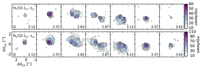
Figure 1.— Channel maps of of H₂CO $3_{12}-2_{11}$ (top), H₂CO $5_{15}-4_{14}$ (bottom) with 0.25 km/s channels. The flux per beam is indicated by the color scales. The line contours are [3,5,7,10,15,20]$\sigma$.

Table 1Observational data

Line	Rest freq.	Log$\rm{}_{10}(A_{ij})$	Eu	beam (PA)	Peak integrated flux	Peak flux
	GHz		K	$\arcsec\times\arcsec$ (∘)	mJy km/s beam-1	mJy beam-1
H2CO $3_{12}-2_{11}$	225.69778	-3.56	33.4	$0\farcs 45\times 0\farcs 45$ ($-75^{\circ}$)	26.7$\pm$2.5	52.8$\pm$2.9
H2CO $5_{15}-4_{14}$	351.76864	-2.43	62.5	$0\farcs 47\times 0\farcs 41$ ($51^{\circ}$)	57.0$\pm$3.9	96.3$\pm$3.8

2.2. H₂CO Spectral Image Cubes

Figure 1 presents channel maps of H₂CO $3_{12}-2_{11}$ and H₂CO $5_{15}-4_{14}$ toward the TW Hya protoplanetary disk. The data was resampled to place the central channel at 2.87 km/s – close to the previously observed systemic velocity of TW Hya (Hughes et al., 2011). Both lines display clear rotation patterns, consistent with a Keplerian disk. The $5_{15}-4_{14}$ emission is more extended than the $3_{12}-2_{11}$ emission, which may be partially a sensitivity issue – the rms noise in the $5_{15}-4_{14}$ data is $\sim$50% higher than in the $3_{12}-2_{11}$ data, but the $5_{15}-4_{14}$ transition is intrinsically an order of magnitude stronger.

Figure 2 shows three different, more condensed visualizations of the H₂CO $3_{12}-2_{11}$ and H₂CO $5_{15}-4_{14}$ data. The top row shows integrated emission or moment-zero maps of the H₂CO emission together with the 1.3 mm continuum. The images were generated in CASA using the immoments task without clipping, and include all channels with any emission above 3$\sigma$ ( 2.12-3.62 km/s for the $3_{12}-2_{11}$ line and 1.87-3.87 for the $5_{15}-4_{14}$ line). Notably, both H₂CO lines display central depressions, but the $3_{12}-2_{11}$ line depression is substantially deeper and appears consistent with a lack of emission at the source center. By contrast, the dust emission is centrally peaked at this spatial resolution.

To decide whether the central emission depressions in H₂CO trace a lack of H₂CO toward the source center we have to exclude three other potential sources: continuum over-subtraction, line opacity, and dust opacity. To address the possibility of continuum over-subtraction, we applied the same continuum subtraction procedure to line free channels and imaged these channels identically to the H₂CO containing channels. We saw no significant emission hole in the resulting image. Second, we estimated the line opacity of both H₂CO lines using the toy models introduced below and find that they are optically thin throughout the disk for all considered abundance profiles. Finally, while we cannot exclude that dust opacity contribute some to the central H₂CO emission depression, it is unlikely to be major contributor. First, observations of other molecules, including CO isotopologues, at similar spatial resolution do not display an emission depression (Schwarz et al., 2016). Second the depression is smaller for the higher frequency transition, where the dust opacity should be higher. We thus conclude that the central depressions in H₂CO emission reflect a real depletion in H₂CO abundance.

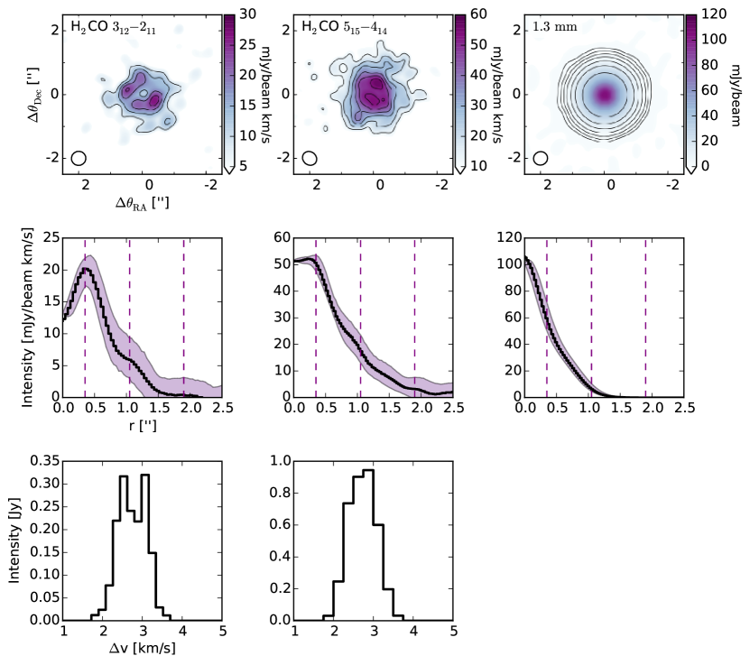
Figure 2.— Overview of observational results. Top row: Integrated emission maps of H₂CO $3_{12}-2_{11}$ (left), H₂CO $5_{15}-4_{14}$ (middle) and 1.3mm dust emission (right). The flux per beam is indicated by the color scales. The line contours are [3,5,7,9,11]$\sigma$ in the H₂CO images, and [4,8,16,32,64,128,256]$\sigma$ in the continuum image. Middle row: Radial profiles of the same H₂CO lines and dust continuum. The shaded region mark the 1$\sigma$ scatter in the intensity values. The three dashed lines mark the observed sub-structure in the H₂CO emission profiles. Bottom row: Extracted spectra using CLEAN masks.

The different emission structures of H₂CO $3_{12}-2_{11}$, H₂CO $5_{15}-4_{14}$, and dust are further visualized in the middle row of Fig. 2, which displays azimuthally averaged radial profiles assuming an inclination of 7 degrees. In addition to the central hole, the $3_{12}-2_{11}$ data show a ‘bump’ around $1\farcs 05$ (62 au), and tentatively a second bump at $1\farcs 9$ (110 au), similar to the location of structure in scattered light observations (van Boekel et al., 2016), indicative of a ringed H₂CO structure in the TW Hya disk. Based on recent ALMA observations, TW Hya hosts a series of dust rings between $0\farcs 02$ and $\sim 1\arcsec$ (1 and 59 au) (Andrews et al., 2016). The observed H₂CO rings and sub-structure do not seem to correspond to any of the most pronounced dust gaps or peaks. The $1\farcs 05$ bump appears to coincide with the edge of the millimeter dust disk, however. This is not the first time that chemical substructure has been observed at the edges of dust disks (Öberg et al., 2015; Huang et al., 2016), hinting at a real chemical change at the edges of large dust/pebble disks. Indeed, in the TW Hya disk, Schwarz et al. (2016) found that there are CO isotopologue bumps at the same $1\farcs 05$ disk location. This chemical change could be driven either by increased UV penetration (Öberg et al., 2015) or a temperature inversion (Cleeves, 2016). The $5_{15}-4_{14}$ emission show similar, but less pronounced, radial structures compared to the H₂CO $3_{12}-2_{11}$ emission, and appears remarkably similar to the $5_{15}-4_{14}$ emission profile previously observed toward the DM Tau disk (Loomis et al., 2015).

The third row of Fig 2 shows the extracted spectra. For the spectra, the native spectral resolution was used rather than 0.25 km/s, which explains some of the different shapes of the two lines. The spectra were extracted from the spectral image cube using the CLEAN mask, and then summing up the emission in each channel. The resulting spectra provide a good measure of the total flux, but do not have any well-defined noise properties, and the total line fluxes and uncertainties listed in Table 1 are instead extracted from integrated flux maps without any clipping applied.

3. H₂CO Toy Models

There are multiple approaches in the literature for extracting information on molecular abundance profiles, including abundance retrieval using grids of parametric models (Qi et al., 2011; Öberg et al., 2012; Qi et al., 2013a; Öberg et al., 2015, e.g.) and Monte Carlo methods (Teague et al., 2015; Guzmán et al., 2017), comparison between observed emission and astrochemistry disk model predictions (Dutrey et al., 2007; Teague et al., 2015; Cleeves et al., 2015), and toy models (Andrews et al., 2012; Rosenfeld et al., 2013). Since we are in an exploratory phase for organic ice chemistry in disks, we adopt the latter approach in this study. Grid and MCMC methods by necessity rely on the assumption that the model being tested has the correct form, locking down the kind of model considered. In light of the wealth of substructure seen in both the present H₂CO data and many other disks and molecules, it is not clear that we know what that form should be for individual disks and molecules. With that in mind, we present a series of toy models of increasing complexity to explore what families of H₂CO abundance structures are qualitatively consistent with the radial profiles and relative intensities of the observed H₂CO lines. We then compare these structures with previously published outputs of detailed astrochemistry codes in the next section.

In our model framework, H₂CO abundances are defined with respect to a pre-existing disk density and temperature model, developed to fit the TW Hya SED and the disk continuum emission (Qi et al., 2013a). Briefly, the adopted TW Hya disk model is a steady viscous accretion disk, heated by irradiation from the central star and by accretion (D’Alessio et al., 1999, 2001, 2006). The disk model is axisymmetric, in vertical hydrostatic equilibrium, and the viscosity follows the $\alpha$ prescription (Shakura & Sunyaev, 1976). Energy is distributed through the disk by radiation, convection, and a turbulent energy flux. The penetration of the stellar and shock generated radiation is calculated, and takes into account scattering and absorption by dust grains. Qi et al. (2013a) added a tapered exponential edge to the standard realization of this model framework to simulate viscous spreading (Hartmann et al., 1998; Hughes et al., 2008; Qi et al., 2011). Following Qi et al. (2011), Qi et al. (2013a) also modified the vertical temperature and density structure by changing the vertical distribution of large grains (D’Alessio et al., 2006). Qi et al. (2013a) explored several different vertical dust grain distributions, of which we selected the intermediate case shown in the upper panels of Fig. 3. It is important to note that despite decades of modeling, disk vertical temperature structures remain highly uncertain. We emphasize that until this uncertainty has been addressed, it is difficult to constrain the vertical emission layer of molecules in absolute terms, or derive accurate H₂CO abundances. As shown below, we can, however, constrain important properties of the emitting layer without knowing the exact layer height. We also note that our model does not take into account the possible presence of a break in the thermal structure at the edge of the pebble disk (Cleeves, 2016), which could results in an underestimate of the temperature in the outer disk by 10%–30%. It is also worth noting that the model was constructed before the recent publication of a revised distance estimate to TW Hya (Gaia Collaboration et al., 2016), which somewhat affects the inferred disk physical parameters, but has a negligible impact on the conclusions of this study.

The physical disk model is populated with H₂CO using one of the parametric prescriptions described below. The level populations of observed lines are computed using RADMC-3D version 0.39 (Dullemond, 2012), assuming the gas is at local thermal equilibrium (LTE). The critical densities of the $3_{12}-2_{11}$ and $5_{15}-4_{14}$ lines are $7\times 10^{5}$ and $2.6\times 10^{6}$ cm^-3, respectively, at 20 K (Shirley, 2015). Apart from the disk atmosphere, typical disk densities are above $1\times 10^{6}$ cm^-3, justifying our assumption of LTE. We used the vis_sample package to compute the Fourier Transform of the synthetic model and sample visibilities at the u – v points of the observations. We finally integrate the emission and calculate the radial profiles using the same procedure as for observations.

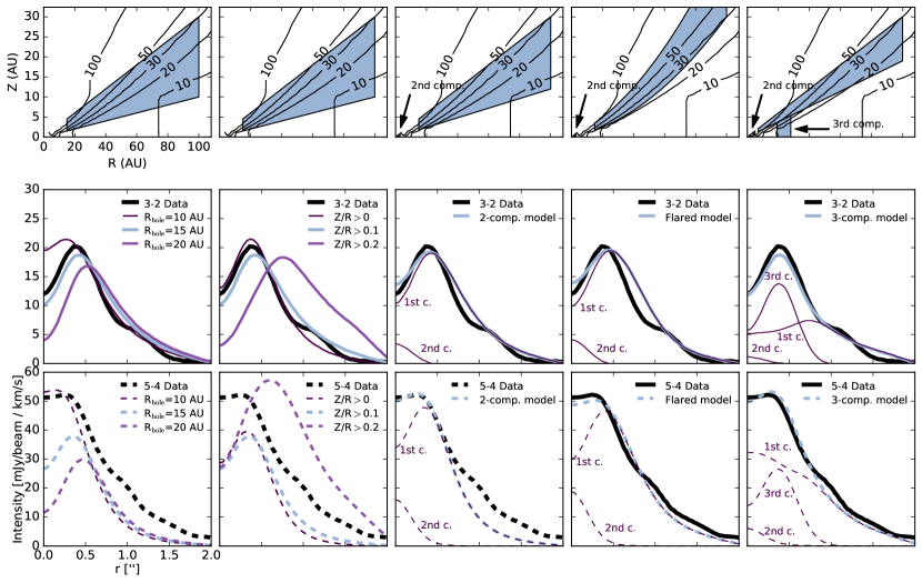
Figure 3.— Parametric toy model H₂CO distributions (top row) and the corresponding calculated $3_{12}-2_{11}$ and $5_{15}-4_{14}$ emission radial profiles (middle and bottom rows), shown together with observed profiles. In the toy model panel, the locations of H₂CO is marked by pale blue. Within each region the H₂CO abundance is either constant or set by a power law. The first two columns show the S1 model and the following three models the 2-component, flared and 3-component models. S2-S5 are not not shown explicitly in the top row. In the bottom two rows, the first column compares model outcomes with different inner holes (model S1-S3), the second column the effects of different vertical profiles (model S1, S4, S5), and the third and fourth columns the improvements obtained by switching from a single component model to a two or three component model. Note the change in x-axis units from AU to arc seconds between the top row and the bottom two rows. All model parameters are listed in Table 2,

Table 2H₂CO toy model parameters

Parameter	Description	S1	S2	S3	S4	S5	2-comp.	Flared	3-comp.
Component 1:
$x_{\rm 1AU}$	abund. at 1 AU [10-9 $n_{\rm H}$]	$8$	$7$	10	0.3	500	120	0.2	430
$\gamma$	power law index	-1.5	-1.5	-1.5	-1.5	-1.5	-2.0	0.0	-1.7
$r_{\rm in}$	inner boundary [AU]	15	10	20	15	15	15	15	7
$r_{\rm out}$	outer boundary [AU]	100	100	100	100	100	100	100	100
$(z/r)_{\rm low}$	midplane boundary at $r_{\rm in}$	0.1	0.1	0.1	0.0	0.2	0.12	0.11	0.19
$(z/r)_{\rm up}$	surface boundary at $r_{\rm in}$	0.3	0.3	0.3	0.3	0.3	0.3	0.23	0.3
Component 2:
$x_{\rm c2}$	inner disk abundance [10-9 $n_{\rm H}$]	–	–	–	–	–	16	20	0.3
Component 1 in flaring 2-comp.model:
$(z/r)_{\rm low}$	midplane boundary at $r_{\rm out}$	–	–	–	–	–	–	0.3	–
$(z/r)_{\rm up}$	surface boundary at $r_{\rm out}$	–	–	–	–	–	–	0.5	–
Component 3:
$x_{\rm c3}$	abundance [10-9 $n_{\rm H}$]	–	–	–	–	–	–	–	0.01
$r_{\rm c3,in}$	inner boundary [AU]	–	–	–	–	–	–	–	19
$r_{\rm c3,out}$	outer boundary [AU]	–	–	–	–	–	–	–	28
$(z/r)_{\rm c3,low}$	lower boundary [AU]	–	–	–	–	–	–	–	0.0
$(z/r)_{\rm c3,up}$	upper boundary [AU]	–	–	–	–	–	–	–	0.19

3.1. Single component models

We begin by considering one of the simplest possible distributions for H₂CO: a single abundance power law $x(r)=x_{\rm 1AU}\times r^{\gamma}$, confined by an inner and outer cut-off radius and a lower and upper boundary. The abundance $x$ is with respect to the total number of hydrogen nuclei per cm^-3, $r$ is the distance from the star in AU, and $\gamma$ a power law index. The lower and upper boundaries are defined by a constant $z/r$, where $z$ is the disk height above the midplane in AU. We fix the upper $(z/r)_{\rm up}$ and outer ($r_{\rm out}$) boundaries to 0.3 and 100 AU, respectively. We initially explored higher upper boundaries, and found that H₂CO emission from more elevated disk regions was negligible as long as the lower boundary in term of $z/r$ is 0.2 or lower. The outer 100 AU boundary corresponds to the estimated outer edge of H₂CO emission in TW Hya. We then vary the inner and lower boundaries, as well as the power law parameters, to explore whether such a simple model can reproduce the observed H₂CO emission profiles, including the observed central depressions. As shown in Fig. 3 (left two columns), a model with an inner radius of 15 AU and a lower layer boundary of 0–0.1 $z/r$ fits the shape of the observed $3_{12}-2_{11}$ radial profile quite well when adopting $\gamma=-1.5$. However, this model cannot reproduce the H₂CO $5_{15}-4_{14}$ radial profile flux level or shape. The predicted $5_{15}-4_{14}$ flux is too low at all radii, and the shape of the radial profile is wrong: compared to the observed $5_{15}-4_{14}$ emission the model depression toward the center is too deep, and in the outer disk the model profile falls off too steeply with radius.

To test whether other versions of the single-component power-law model could reproduce both the $3_{12}-2_{11}$ and $5_{15}-4_{14}$ emission, we set up a small grid of toy models varying the inner hole radius, the lower boundary of the emitting layer, and the power law index. For each model we select a inner radius and a lower layer boundary, and then adjust the power law coefficient and $x_{\rm 1AU}$ to obtain a reasonable ‘by-eye’ fit to the H₂CO $3_{12}-2_{11}$ emission. The two left-hand columns of Fig. 3 show a sub-set of these models, focusing on the inner radius (first column), and the emitting layer location (second column). The model parameters are listed in Table 2 as S1-5 (where S stands for ‘single component model’). It is not possible to simultaneously reproduce the $3_{12}-2_{11}$ central hole, and the almost flat central profile of the $5_{15}-4_{14}$ emission with a single inner radius. The $5_{15}-4_{14}$ emission is also always under-predicted in the outer disk for the models that can reproduce the $3_{12}-2_{11}$ emission; that discrepancy increases with radius. This cannot be fixed by a uniform increase in the lower boundary since the required increase in $(z/r)_{\rm low}$ produces a H₂CO depression that extends farther out than is observed. It also cannot be explained by a radially dependent ortho-to-para ratio, since both lines are ortho lines. A single-component parametric model appears to be ruled out by the data.

3.2. Two- and three-component models

First, consider the mismatch at small radii. Since the $3_{12}-2_{11}$ emission requires a considerable H₂CO abundance deficit and the $5_{15}-4_{14}$ emission profile requires some H₂CO on scales of 10 AU or less, it appears that the only way to reconcile the two is to add a hot unresolved H₂CO component that primarily contributes to the $5_{15}-4_{14}$ emission. We achieve this by adding a second H₂CO component between 1 and 3 AU, and between $z/r$ of 0.1 and 0.3 (Fig. 3, third column). For simplicity, we set the H₂CO abundance to be constant in this layer. By adjusting the abundances in the hot component and the outer disk component, this model can reproduce the radial shapes and relative intensity levels of the $3_{12}-2_{11}$ and $5_{15}-4_{14}$ emission out to $\sim$0$\farcs$6 (Table 2, 2-comp. model). Beyond this radius, the $5_{15}-4_{14}$ emission is always underproduced.

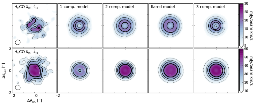
Figure 4.— Observed (first column) and simulated (column 2–5) H₂CO emission. The second column shows a single component power law model (S1 in Table 2), the third column a 2-comp. model with a central hot component, the fourth column a flaring 2-comp. model and the fifth column a 3-comp. model, where the 3rd component constitutes a ring of emission between 19 and 28 AU. All model parameters are listed in Table 2,

Second, consider the mismatch at large radii. There is a radially increasing mismatch between predicted and observed $5_{15}-4_{14}$ emission for the models considered so far. This suggests that H₂CO is present in a warmer emitting region in the outer disk than what is achieved by constant $z/r$ boundaries. In the context of the adopted temperature profile, this implies that H₂CO is present in a more elevated layer (in units of $z/r$) in the outer disk compared to the emission peak at $\sim$0$\farcs$4. We consider two different parameterizations that could address this: a flaring H₂CO power law model (Fig. 3, fourth column) and a three-component model (Fig. 3, right-hand column). In the flaring H₂CO model, the lower and upper boundaries in units of $z/r$ increase linearly with radius between 15 and 100 AU. In the three component model, a midplane ring at 19–28 AU (3rd component) is combined with a power law abundance model at elevated, and therefore warm, disk layers ($z/r=0.19-0.3$) to produce excess $5_{15}-4_{14}$ emission in the outer disk. Both kinds of parameterizations can be set up to reproduce the overall radial shapes and relative emission levels of the $3_{12}-2_{11}$ and $5_{15}-4_{14}$ lines (Fig. 3). The model parameters that best reproduce observations (by eye) are listed in Table 2.

3.3. Model comparison

The failure of the single power law models, and the simple 2-component model to reproduce the shape of the $5_{15}-4_{14}$ emission is also clearly seen in Fig. 4, which shows integrated emission maps. As expected from the radial profile comparisons: the ‘optimized’ flared H₂CO abundance model and the 3-comp. model reproduce the main features of the emission from both lines very well. It is important to note, however, that despite the close resemblance of observed and model emission, none of the toy models provide a good quantitative fit when comparing channel maps; there are significant residuals ($>5\sigma$). This is unsurprising, considering that these are toy models, but it emphasizes that the presented models should not be viewed as the final word on how H₂CO is distributed in the TW Hya disk. Rather, this exercise provides initial constraints on what families of models are consistent with the observations.

In summary, the toy models demonstrate that the $3_{12}-2_{11}$ emission requires a depleted H₂CO abundance in the inner disk, while the $5_{15}-4_{14}$ emission requires some H₂CO to still be present there. This can be resolved if a H₂CO depletion is combined with a hot H₂CO component close to the star. The relative intensities of the two lines imply that H₂CO is vertically located close to the midplane (i.e. a lower boundary of 0-0.1 $z/r$) at intermediate disk radii, beginning around 15 AU, and at more elevated disk layers at larger radii, beyond 60 au. In the context of the adopted temperature structure, this can be parameterized with either a flaring H$2$CO layer or with a 3-component model with constant $z/r$ vertical boundaries for each component. None of these models reproduce the observed emission bump at 1$\farcs$05, which would require a fourth model component.

4. Discussion

4.1. H₂CO abundance structure

The H₂CO $3_{12}-2_{11}$ and $5_{15}-4_{14}$ line emission profiles in TW Hya belong to an increasingly large class of molecular lines that appear as emission rings in disks. Previous molecular emission rings have either been connected to dust deficiencies (e.g. Zhang et al., 2014; Öberg et al., 2015), temperature or photon regulated gas-phase chemistry (e.g. Aikawa et al., 2003; Qi et al., 2008; Bergin et al., 2016), or snowlines (Qi et al., 2013a, b).

In the case of H₂CO in TW Hya, we have demonstrated that the observed H₂CO emission profiles require an underlying abundance structure that fulfills the following conditions: 1) a distinct inner disk H₂CO component that is warm, 2) a second mid-to-outer disk component of H₂CO, where 3) the emitting layer resides at higher $z/r$ in the outer disk ($r>60$ AU) compared the to intermediate disk radii ($15<r<30$ AU). The last condition is a result of the presence of a high H₂CO $5_{15}-4_{14}$/$3_{12}-2_{11}$ intensity ratio in the outer disk. This implies a relatively warm H₂CO emitting layer in the outer disk, which in the adopted disk temperature model occurs at $z/r>0.2$.

It is not clear, however, that the adopted temperature structure provides a good description of the TW Hya disk temperatures beyond the millimeter dust disk. Cleeves (2016) found that the loss of millimeter grains in the outer disk will cause a temperature inversion, substantially increasing the temperature in the outer disk. There is observational evidence that this takes place in other disks (Huang et al., 2016), and it may well affect the TW Hya outer disk temperature profile. If a temperature inversion is present at the millimeter disk edge in TW Hya, two effects on the H₂CO emission may be expected: a change in the slope of all H₂CO intensity profiles around the dust edge where the temperature inversion occurs, and excess $5_{15}-4_{14}$ emission everywhere in the outer disk, since the overall temperature will be elevated compared to standard disk modeling assumptions where the temperature monotonically decreases with radius. Both features are observed in the TW Hya disk, which is highly suggestive. Furthermore, Schwarz et al. (2016) suggests that a bump in the CO emission at this radius may trace a second snowline, as would be expected if a temperature inversion is present. Better constraints on the outer disk temperature profile are needed before we can present a conclusive interpretation of the H₂CO outer disk emitting layer. In the meantime, we cannot tell whether the observed excess $5_{15}-4_{14}$ emission is due to an elevated emitting layer in the outer disk or excess temperatures in the outer disk compared to our adopted temperature structure.

In the inner disk, it is interesting to compare the location of the H₂CO inner radius and the CO snowline, since one of the proposed H₂CO formation pathways in disks is through CO ice hydrogenation. The CO snowline location is inferred from N₂H⁺ observations to be at 30 AU (Qi et al., 2013b). This is considerably outside of the 15–20 AU boundary where H₂CO first appears in the TW Hya disk (ignoring the inner hot component). However, this difference does not automatically exclude an icy origin of the outer disk H₂CO because the onset and completion of CO condensation can occur at different temperatures and therefore different disk locations. H₂CO ice formation is expected to become efficient at the onset of CO freeze-out, which is likely regulated by the temperature at which CO binds to H₂O ice. N₂H⁺ gas-phase production becomes efficient when most CO has been depleted from the gas-phase, which is likely regulated by the lower CO:CO ice binding energy (Collings et al., 2003; Fayolle et al., 2016), since there should be sufficient CO in disks to form multi-layered CO ices in the outer disk. Furthermore, H₂CO formation on grains can begin at even higher grain temperatures than expected for CO freeze-out on water ice, since it only requires that some of the CO spends some of their time on grains. Based on these two considerations alone we would expect a substantial difference between the H₂CO inner radius and the CO snowline location, defined as the location where CO freeze-out nears completion. In addition, a recent study shows that the inner radius of N₂H⁺ rings only provides an upper limit to the CO snowline (van ’t Hoff et al., 2016). It is therefore possible that the CO snowline location in Qi et al. (2013b) is overestimated by several AU. In light of these laboratory and theoretical results a large difference between the H₂CO and the N₂H⁺ inner edges is compatible with the proposed icy origin of H₂CO in the outer disk.

4.2. H₂CO formation in the TW Hya disk

H₂CO formation through gas and grain surface chemistry has been explored theoretically in a number of models (e.g. Aikawa et al., 2003; Aikawa & Nomura, 2006; Willacy, 2007; Willacy & Woods, 2009; Walsh et al., 2014). Most recently, Loomis et al. (2015) modeled the H₂CO abundance in a T Tauri disk with gas and grain surface formation, and with either gas or grain surface formation turned off. We focus our comparison on the three models that show the predicted H₂CO abundance structure in detail: Willacy & Woods (2009), Walsh et al. (2014), and Loomis et al. (2015).

These three H₂CO model predictions share a number of important features. All contain a central H₂CO component, which is attributed to gas-phase formation of H₂CO. The extent of the inner component depends on the details of adopted disk model, but is generally concentrated within 10 AU. All models also predict an outer disk H₂CO component at intermediate disk heights $0.2<z/r<0.4$. In Loomis et al. (2015), the inner and outer disk component connect, while in Willacy & Woods (2009) and Walsh et al. (2014) the inner and outer disk components are distinct. This second component is explained by grain-surface formation of H₂CO. The component consists of a disk layer that is cold enough for CO to have a substantial residence time on grains, enabling hydrogenation to form H₂CO, and low-density enough for non-thermal desorption to maintain some of the formed H₂CO in the gas, either through release of chemical energy or photodesorption.

In addition to these two components, Willacy & Woods (2009) and Walsh et al. (2014) predict a third, radially confined component close to the midplane at $\sim$20 AU. This component also appears to be due to grain surface formation followed by non-thermal desorption, and represents the midplane location where CO begins to reside for substantial amounts of time on grain surfaces. The lack of this component in Loomis et al. (2015) may reflect different assumptions of radiation fields and desorption efficiencies in that model.

The observationally constrained H₂CO abundance structure in the TW Hya disk qualitatively agrees these model predictions. It is important to note, however, that non-thermal ice desorption efficiences are highly uncertain. As a result, the model predictions in the outer disk that rely on these pathways are order of magnitude estimates, at best. Gas-phase chemistry will also continue to contribute to the overall H₂CO abundances throughout the disk through e.g. the very efficient CH₃+O reaction (Atkinson et al., 2006). The relative importance of grain and gas-phase chemistry in the outer disk of TW Hya is therefore difficult to quantify with certainty based on extracted column densities. The radial H₂CO abundance profiles provide stronger constraints, and the observed H₂CO emission profile in TW Hya is only expected if the grain-surface formation and desorption pathway produces the majority of the observed H₂CO exterior to 15 AU. Beyond that, it is not possible with the present data to distinguish between different model predictions, since the data are consistent both with a single flaring component in the outer disk (similar to Loomis et al. (2015), and a 3-component model, where the third component traces the midplane onset of H₂CO ice formation (similar to Willacy & Woods (2009) and Walsh et al. (2014) ). Higher resolution data and a better constrained disk temperature profile used both for retrieval and chemistry model predictions are needed to resolve whether this third component is present in the TW Hya disk.

In either case, considering the good agreement between observational constraints on the H₂CO distribution in the TW Hya disk and astrochemical disk model predictions we can put some qualitative constraints on the H₂CO chemistry in the TW Hya disk. H₂CO forms close to the star due to warm gas-phase chemistry. If pebble drift is efficient, additional H₂CO gas may be delivered to the inner disk gas as the pebbles cross the H₂CO snowline (e.g. Öberg & Bergin, 2016). These processes enrich the gas in the terrestrial planet forming zone in gas-phase H₂CO. There is then a H₂CO chemistry desert until grain-surface chemistry kicks in around 15-20 AU through hydrogenation of CO ice, with some possible minor contribution from gas-phase chemistry. Further out in the disk, H₂CO ice continues to form at all disk heights where the temperature is sufficiently low, but H₂CO is only released efficiently into the gas-phase at intermediate to high disk layers, where non-thermal desorption is most efficient.

In this scenario, we expect that CH₃OH would follow the H₂CO distribution, except it should lack the central component tracing gas-phase H₂CO formation chemistry. So far, only low-SNR observations of CH₃OH exist (Walsh et al., 2016). The data favor a central cavity in the CH₃OH abundance distribution, but the size of the cavity or the location of the emitting layer was not constrained. Higher SNR data are needed to provide a direct test of this prediction.

5. Conclusions

Using a series of toy models we demonstrated that to simultaneously reproduce the observed H₂CO $3_{12}-2_{11}$ and $5_{15}-4_{14}$ emission requires a distinct hot H₂CO gas reservoir in the inner disk, and an extended H₂CO gas reservoir in the outer disk. The resulting two-component H₂CO model only reproduces the outer disk emission of both H₂CO lines if the H₂CO emitting layer increases in height (in terms of $z/r$) with radius, or if there is a hitherto undetected temperature inversion in the disk at the millimeter dust edge. The model approach thus informed us on what families of models that are consistent with the data. It is important to note that if only one of the two lines had been observed, the data would have been consistent with a single power law distribution, resulting in very different conclusions on the radial and vertical distribution of H₂CO in this disk.

The inferred H₂CO structure is qualitatively consistent to what is predicted by astrochemical disk codes that includes both warm gas-phase chemistry and cold hydrogenation of CO on grains. This implies that similar to the much younger DM Tau system, the old TW Hya disk hosts an active gas-phase and grain-surface organic chemistry. This active disk chemistry should result in a time dependent organic composition in disks. It is thus likely that planetesimals assembling at different times during the lifetime of the disk will acquire different chemical compositions, and in particular different abundances of simple and complex organic molecules.

References

- Aikawa et al. (2003) Aikawa, Y., Momose, M., Thi, W., et al. 2003, PASJ, 55, 11
- Aikawa & Nomura (2006) Aikawa, Y., & Nomura, H. 2006, ApJ, 642, 1152
- Andrews et al. (2012) Andrews, S. M., Wilner, D. J., Hughes, A. M., et al. 2012, ApJ, 744, 162
- Andrews et al. (2016) Andrews, S. M., Wilner, D. J., Zhu, Z., et al. 2016, ApJ, 820, L40
- Atkinson et al. (2006) Atkinson, R., Baulch, D. L., Cox, R. A., et al. 2006, Atmos. Chem. Phys., 6, 3625
- Bennett et al. (2007) Bennett, C. J., Chen, S.-H., Sun, B.-J., Chang, A. H. H., & Kaiser, R. I. 2007, ApJ, 660, 1588
- Bergin et al. (2015) Bergin, E. A., Blake, G. A., Ciesla, F., Hirschmann, M. M., & Li, J. 2015, Proceedings of the National Academy of Science, 112, 8965
- Bergin et al. (2016) Bergin, E. A., Du, F., Cleeves, L. I., et al. 2016, ArXiv e-prints, arXiv:1609.06337
- Boyer et al. (2016) Boyer, M. C., Rivas, N., Tran, A. A., Verish, C. A., & Arumainayagam, C. R. 2016, Surface Science, 652, 26
- Carr & Najita (2008) Carr, J. S., & Najita, J. R. 2008, Science, 319, 1504
- Cleeves (2016) Cleeves, L. I. 2016, ApJ, 816, L21
- Cleeves et al. (2015) Cleeves, L. I., Bergin, E. A., Qi, C., Adams, F. C., & Öberg, K. I. 2015, ApJ, 799, 204
- Collings et al. (2003) Collings, M. P., Dever, J. W., Fraser, H. J., & McCoustra, M. R. S. 2003, Ap&SS, 285, 633
- Cuppen et al. (2009) Cuppen, H. M., van Dishoeck, E. F., Herbst, E., & Tielens, A. G. G. M. 2009, A&A, 508, 275
- D’Alessio et al. (2001) D’Alessio, P., Calvet, N., & Hartmann, L. 2001, ApJ, 553, 321
- D’Alessio et al. (2006) D’Alessio, P., Calvet, N., Hartmann, L., Franco-Hernández, R., & Servín, H. 2006, ApJ, 638, 314
- D’Alessio et al. (1999) D’Alessio, P., Calvet, N., Hartmann, L., Lizano, S., & Cantó, J. 1999, ApJ, 527, 893
- Dullemond (2012) Dullemond, C. P. 2012, RADMC-3D: A multi-purpose radiative transfer tool, Astrophysics Source Code Library, , , ascl:1202.015
- Dutrey et al. (1997) Dutrey, A., Guilloteau, S., & Guelin, M. 1997, A&A, 317, L55
- Dutrey et al. (2007) Dutrey, A., Henning, T., Guilloteau, S., et al. 2007, A&A, 464, 615
- Fayolle et al. (2016) Fayolle, E. C., Balfe, J., Loomis, R., et al. 2016, ApJ, 816, L28
- Fuchs et al. (2009) Fuchs, G. W., Cuppen, H. M., Ioppolo, S., et al. 2009, A&A, 505, 629
- Gaia Collaboration et al. (2016) Gaia Collaboration, Brown, A. G. A., Vallenari, A., et al. 2016, ArXiv e-prints, arXiv:1609.04172
- Gerakines et al. (1996) Gerakines, P. A., Schutte, W. A., & Ehrenfreund, P. 1996, A&A, 312, 289
- Guzmán et al. (2017) Guzmán, V. V., Öberg, K. I., Huang, J., Loomis, R., & Qi, C. 2017, ApJ, 836, 30
- Hartmann et al. (1998) Hartmann, L., Calvet, N., Gullbring, E., & D’Alessio, P. 1998, ApJ, 495, 385
- Högbom (1974) Högbom, J. A. 1974, A&AS, 15, 417
- Huang et al. (2016) Huang, J., Öberg, K. I., & Andrews, S. M. 2016, ApJ, 823, L18
- Hudson & Moore (2000) Hudson, R. L., & Moore, M. H. 2000, Icarus, 145, 661
- Hughes et al. (2011) Hughes, A. M., Wilner, D. J., Andrews, S. M., Qi, C., & Hogerheijde, M. R. 2011, ApJ, 727, 85
- Hughes et al. (2008) Hughes, A. M., Wilner, D. J., Qi, C., & Hogerheijde, M. R. 2008, ApJ, 678, 1119
- Kastner et al. (1997) Kastner, J. H., Zuckerman, B., Weintraub, D. A., & Forveille, T. 1997, Science, 277, 67
- Le Roy et al. (2015) Le Roy, L., Altwegg, K., Balsiger, H., et al. 2015, A&A, 583, A1
- Loomis et al. (2015) Loomis, R. A., Cleeves, L. I., Öberg, K. I., Guzman, V. V., & Andrews, S. M. 2015, ApJ, 809, L25
- Morbidelli et al. (2012) Morbidelli, A., Lunine, J. I., O’Brien, D. P., Raymond, S. N., & Walsh, K. J. 2012, Annual Review of Earth and Planetary Sciences, 40, 251
- Mumma & Charnley (2011) Mumma, M. J., & Charnley, S. B. 2011, ARA&A, 49, 471
- Öberg (2016) Öberg, K. I. 2016, Chemical Reviews, 116, 9631
- Öberg & Bergin (2016) Öberg, K. I., & Bergin, E. A. 2016, ApJ, 831, L19
- Öberg et al. (2015) Öberg, K. I., Furuya, K., Loomis, R., et al. 2015, ApJ, 810, 112
- Öberg et al. (2009) Öberg, K. I., Garrod, R. T., van Dishoeck, E. F., & Linnartz, H. 2009, A&A, 504, 891
- Öberg et al. (2012) Öberg, K. I., Qi, C., Wilner, D. J., & Hogerheijde, M. R. 2012, ApJ, 749, 162
- Öberg et al. (2010) Öberg, K. I., Qi, C., Fogel, J. K. J., et al. 2010, ApJ, 720, 480
- Öberg et al. (2011) —. 2011, ApJ, 734, 98
- Powner et al. (2009) Powner, M. W., Gerland, B., & Sutherland, J. D. 2009, Nature, 459, 239
- Qi et al. (2011) Qi, C., D’Alessio, P., Öberg, K. I., et al. 2011, ApJ, 740, 84
- Qi et al. (2013a) Qi, C., Öberg, K. I., Wilner, D. J., & Rosenfeld, K. A. 2013a, ApJ, 765, L14
- Qi et al. (2008) Qi, C., Wilner, D. J., Aikawa, Y., Blake, G. A., & Hogerheijde, M. R. 2008, ApJ, 681, 1396
- Qi et al. (2006) Qi, C., Wilner, D. J., Calvet, N., et al. 2006, ApJ, 636, L157
- Qi et al. (2013b) Qi, C., Öberg, K. I., Wilner, D. J., et al. 2013b, Science, 341, 630
- Raymond et al. (2014) Raymond, S. N., Kokubo, E., Morbidelli, A., Morishima, R., & Walsh, K. J. 2014, Protostars and Planets VI, 595
- Rosenfeld et al. (2013) Rosenfeld, K. A., Andrews, S. M., Wilner, D. J., Kastner, J. H., & McClure, M. K. 2013, ApJ, 775, 136
- Schwarz et al. (2016) Schwarz, K. R., Bergin, E. A., Cleeves, L. I., et al. 2016, ApJ, 823, 91
- Shakura & Sunyaev (1976) Shakura, N. I., & Sunyaev, R. A. 1976, MNRAS, 175, 613
- Shirley (2015) Shirley, Y. L. 2015, PASP, 127, 299
- Sullivan et al. (2016) Sullivan, K. K., Boamah, M. D., Shulenberger, K. E., et al. 2016, MNRAS, 460, 664
- Teague et al. (2015) Teague, R., Semenov, D., Guilloteau, S., et al. 2015, A&A, 574, A137
- Thi et al. (2004) Thi, W., van Zadelhoff, G., & van Dishoeck, E. F. 2004, A&A, 425, 955
- van Boekel et al. (2016) van Boekel, R., Henning, T., Menu, J., et al. 2016, ArXiv e-prints, arXiv:1610.08939
- van der Marel et al. (2014) van der Marel, N., van Dishoeck, E. F., Bruderer, S., & van Kempen, T. A. 2014, A&A, 563, A113
- van ’t Hoff et al. (2016) van ’t Hoff, M. L. R., Walsh, C., Kama, M., Facchini, S., & van Dishoeck, E. F. 2016, ArXiv e-prints, arXiv:1610.06788
- Walsh et al. (2014) Walsh, C., Millar, T. J., Nomura, H., et al. 2014, A&A, 563, A33
- Walsh et al. (2016) Walsh, C., Loomis, R. A., Öberg, K. I., et al. 2016, ApJ, 823, L10
- Watanabe & Kouchi (2002) Watanabe, N., & Kouchi, A. 2002, ApJ, 567, 651
- Willacy (2007) Willacy, K. 2007, ApJ, 660, 441
- Willacy & Woods (2009) Willacy, K., & Woods, P. M. 2009, ApJ, 703, 479
- Zhang et al. (2014) Zhang, K., Isella, A., Carpenter, J. M., & Blake, G. A. 2014, ApJ, 791, 42