Statistics, distillation, and ordering emergence in a two-dimensional stochastic model of particles in counterflowing streams

Abstract

In this paper, we proposed a stochastic model which describes two species of particles moving in counterflow. The model generalizes the theoretical framework describing the transport in random systems since particles can work as mobile obstacles, whereas particles of one species move in opposite direction to the particles of the other species, or they can work as fixed obstacles remaining in their places during the time evolution. We conducted a detailed study about the statistics concerning the crossing time of particles, as well as the effects of the lateral transitions on the time required to the system reaches a state of complete geographic separation of species. The spatial effects of jamming were also studied by looking into the deformation of the concentration of particles in the two-dimensional corridor. Finally, we observed in our study the formation of patterns of lanes which reach the steady state regardless the initial conditions used for the evolution. A similar result is also observed in real experiments involving charged colloids motion and simulations of pedestrian dynamics based on Langevin equations, when periodic boundary conditions are considered (particles counterflow in a ring symmetry). The results obtained through Monte Carlo numerical simulations and numerical integrations are in good agreement with each other. However, differently from previous studies, the dynamics considered in this work is not Newton-based, and therefore, even artificial situations of self-propelled objects should be studied in this first-principle modeling.

1 Introduction

In condensed matter physics, the study of the transport of particles in random environments under quenched or annealed scenarios has a huge number of applications such as the capture/decapture of electrons in the micro/nano/meso devices [1, 2, 3], the random motion of molecular motors in the cellular transport (see, for example, Ref. [4]), the erratic motion of molecules in cromatographic columns [5] and many others. Among these problems, one in particular called our attention: the counterflowing streams of particles, which can appear in many contexts due to its importance, for instance, in the separation of chemical products [6], pedestrian dynamics [11, 12, 13, 14, 15, 18, 7], and band formation in mixtures of oppositely charged colloids [16, 17].

Recently, more precisely in the context of pedestrian dynamics, some authors have studied the problem by considering the equation of motion for each particle as a Langevin-like equation [7] which uses the known and successful approach of social force developed by Helbing and Molnár in 1995 [12]. Basically, such approach defines that the dynamics depends on deterministic and stochastic forces. They considered a stokesian drag force that imposes velocities on the particles, an interaction force (repulsion) among particles, an interaction force of particles with the system boundaries, and a Gaussian noise term (based on the existence of an arbitrary motion in a crowd). The authors [7] have shown that asymmetrically shaped walls in a corridor with pedestrian counterflow can surprisingly organize the flow of pedestrians in two only opposite directions (“keep-left” behavior). In pedestrian dynamics, it is important to observe that lane formation phenomenon in pedestrian counterflow were observed via numerical results in other situations. For instance, in Ref. [[8]], the simulations based on optimal path-choice strategy showed that segregation is associated with the minimization of the travel time to reach the ordering state. Similarly, an extended lattice-gas model under periodic boundary conditions is also able to lead to such lane patterns [9]. Such results are experimentally corroborated by real situations as shown by Kretz et al. [10] by using pedestrian counterflow experiment in a corridor of width 2 m and 67 participants.

In addition, based on the concept of clannish random walks, Montroll and West [19] have given an alternative approach for the study of these problems of counterflowing streams of particles in a special kind of mean-field regime. By making the necessary changes and adaptations, we proposed in Ref. [[18]] a one-dimensional stochastic dynamics based on an embryonic idea of those authors by substituting the effects of social forces and other contributions by the following assumptions: (a) from a microscopic point of view, more than one particle can occupy the same cell and (b) each particle of one species jumps to a neighbor cell with probability which depends on the local concentration of particles of the other species.

By following the experimental results of Vissers et al. [16, 17] about patterns produced by oppositely charged particles under action of electric fields, we are wondering about the minimal ingredients necessary to produce lane patterns in a stochastic dynamics based on occupation of cells. So, in this paper we propose a two-dimensional model in order to describe the motion of two species of particles ($A$ and $B$) moving in opposite directions. In our model, the evacuation probabilities of a given species located on a cell change according to the concentration of the other species on this same cell at that time. This is a general and simple way to model the possible interactions between these particles. Additionally, our model was motivated by the pedestrian dynamics and the stationary cases are compared with alternative models as, for example, that one presented in Ref. [[7]].

The generality of our stochastic modeling offers many alternatives of scenarios as suggested in Fig. 1, and depending on the choice of the parameters, we can apply the model for different situations:

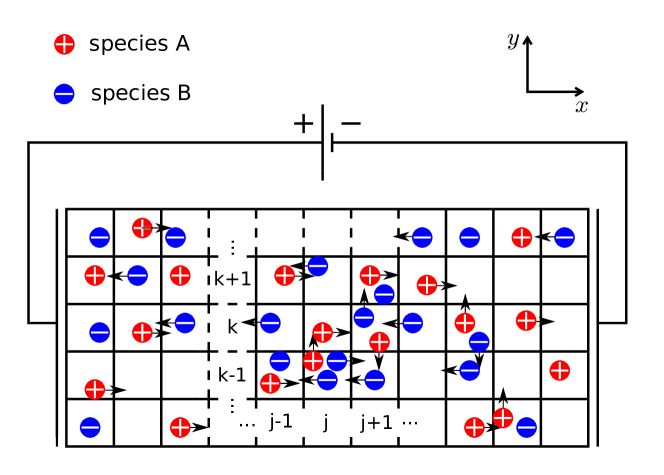
Figure 1: Scheme of the stochastic model of two species of particles in a two-dimensional lattice where the particles can transit to the neighbor cells. In this modeling, the particles $B$ are able to move or can remain in fixed cells considering the flux of the target particles $A$. In a first case (annealed scenario) we are considering conterflowing streams of particles of species $A$ against the species $B$. On the other hand, whe can consider the particles of species $B$ working as fixed obstacles (quenched scenario). In this last case, the motion of particles $A$ is an interesting example of ordered transport of particles with fixed impurities spatially distributed in the environment. The analogy with a charged system and an electric field applied along the longitudinal direction is explored in this figure.

1. Annealed scenario: The species move against each other, for example, $A$ to the right and $B$ to the left composing two counterflowing streams of particles. The two streams interact affecting each other. In a cell, the concentration of particles of a given species changes as time evolves and therefore the transition probabilities of the another species to that cell also change according to this concentration. We can imagine oppositely charged particles under action of electric fields in the context of granular materials [16, 17] etc. So, we can observe jamming effects that emerge due to the resistance of the oppositely charged particles moving in opposite direction, since the motion depends on their concentration per cell. Another interesting example is the motion of the two counterflowing streams of pedestrians in a corridor. In that case, the self-propulsion of the pedestrians into a preferential direction plays the role of the electric field [18, 7];

2. Quenched scenario: The particles $B$ remain in fixed positions chosen at random at the beginning of the time evolution. In this case, the particles of the species $B$ work as obstacles for the particles of species $A$. One can imagine the particles $B$ as fixed impurities in a material and the model can be thought as a traditional random (but directed) walk of particles in a general transport phenomena, exactly as happens in the electrons transport in the interfaces of a semiconductor, chromatograph process of molecules, motion in dopped materials and many others (see for example [3, 5]).

In this paper, we describe the statistical fluctuations and the relaxation process considering different initial conditions in both scenarios considering a rectangular lattice that may or may not have periodic boundary conditions depending on the studied problem. We also show an approach that considers both Monte Carlo (MC) simulations and Numerical Integration (NI) of recurrence equations of the flows of particles along the lattice. The partial differential equations that govern the dynamics at continuum limit are also deduced.

In the annealed scenario we can separate our contribution in three main parts:

1. Statistical characterization of spatial distribution of particles which considers one strip of each species located initially at the opposite extremities of the corridor;

2. By considering the two species randomly mixed in the lattice at the beginning of the evolution, we analyze the fluctuations in the times needed to the complete separation of the two species (distillation);

3. We consider the emergence of ordering by longitudinal bands considering periodic boundary conditions (or simply that the two species can rotate in a ring). We defined an interesting order parameter to quantify the appearance of bands considering the interaction of the counterflowing streams of the two different species.

On the other hand, in the quenched scenario, we concentrate our analysis in measuring the fluctuations on the crossing times of the target particles considering different densities of the fixed particles (obstacles). We observe an interesting crossover for these crossing times that are normally distributed (a limit case of a negative binomial distribution) at low concentration of obstacles and become distributed according to a power law in a transient situation corresponding to an intermediate concentration of obstacles. Finally, exponential tails appear after a high concentration of particles which makes the system very stagnant.

In the next section we explain the details of the modeling and definitions of the order parameters which describe the cellular segregation of the particles in the different studies. In section 3 we present the results related to the situation where one of the species is not able to moove, i.e., the particles of that species is fixed in the cells and work as obstacles for the oriented transport of the target particles (the particles of the other species). In section 4, we present our main results when the two species are oriented in opposite directions forming counterflowing streams of particles. We finally present some summaries and our conclusions in section 6.

2 Methods and modeling

In this model, we consider a corridor with linear dimensions $L_{x}$ and $L_{y}$, the width and length dimensions, respectively, so that we have a total of $L_{x}L_{y}$ cells in this lattice. We take into account particles of species $A$ ($+$) that move preferably to the left and particles of species $B$ ($-$) moving preferably to the right according to, for example, an application of a uniform field (which is supposed to be constant). We denote $\rho_{A}(j,k)=\frac{c_{A}(j,k)}{c_{A}(j,k)+c_{B}(j,k)}$ and $\rho_{B}(j,k)=\frac{c_{B}(j,k)}{c_{A}(j,k)+c_{B}(j,k)}$ as the concentration of particles $A$ and $B$, respectively, in the cell $(j,k)$ with $j=1,\cdots,L_{x}$ and $k=1,\cdots,L_{y}$. Here, $c_{A}$ and $c_{B}$ are, respectively, the total number of particles of the species $A$ and $B$ in the cell.

In the more general context (annealed system), we denote $p$ as the probability that directs the particles of both species, which depends on the applied field. So, the interaction occurs when the counterflowing particles visit the same cells. For the species $A$ this interaction is defined by (the same analysis present below is applied to the species $B$):

$$\begin{array}[]{l}\Pr^{(A)}(j\rightarrow j+1,k\rightarrow k)=p-\alpha\rho_{B}(j,k)\\ \\ \Pr^{(A)}(j\rightarrow j+1,k\rightarrow k\pm 1)=\beta_{\perp}\rho_{B}(j,k)\\ \\ \Pr^{(A)}(j\rightarrow j-1,k\rightarrow k)=\beta_{\parallel}\rho_{B}(j,k)\\ \\ \Pr^{(A)}(j\rightarrow j,k\rightarrow k)=1-p+(\alpha-\beta)\rho_{B}(j,k)\end{array}$$ (1)

where $\beta=\beta_{\perp}+\beta_{\parallel}$. Here $\alpha$ is related to the frontal resistance that particles offer to the reference particles as considered in Ref. [[18]]. The particles can move to the right or to the left with the same probability $\beta_{\perp}\rho_{A}(j,k)$. We introduce an elastic effect that promotes the return of the particle to the previous cell with probability $\beta_{\parallel}\rho_{A}(j,k)$.

By denoting $n_{j,k,l}$ the number of target particles in the cell ($j,k$) at the instant $l$, the first approach leads to the recurrence equation

$$\begin{array}[]{l}n_{j,k,l+1}=n_{j,k,l}-p(n_{j,k,l}-n_{j-1,k,l})\\ \\ +\alpha\left[\left(1-\frac{n_{j,k,l}}{N_{j,k,l}}\right)n_{j,k,l}-\left(1-\frac{n_{j-1,k,l}}{N_{j-1,k,l}}\right)n_{j-1,k,l}\right]\\ \\ +\beta_{\parallel}\left[\left(1-\frac{n_{j+1,k,l}}{N_{j+1,k,l}}\right)n_{j+1,k,l}-\left(1-\frac{n_{j,k,l}}{N_{j,k,l}}\right)n_{j,k,l}\right]\\ \\ +\beta_{\perp}\left[\left(1-\frac{n_{j,k+1,l}}{N_{j,k+1,l}}\right)n_{j,k+1,l}+\left(1-\frac{n_{j,k-1,l}}{N_{j,k-1,l}}\right)n_{j,k-1,l}\right.\\ \\ -\left.2\left(1-\frac{n_{j,k,l}}{N_{j,k,l}}\right)n_{j,k,l}\right].\end{array}$$ (2)

where $N_{j,k,l}=n_{j,k,l}+m_{j,k,l}$ is the total of particles in the cell ($j,k$) at the instant $t=l\Delta$ and $m_{j,k,l}$ is the number of opposite particles in the same cell and instant.

This corresponds to the discretizations of the EDP:

$$\frac{\partial c_{A}}{\partial t}=-k_{1}\frac{\partial c_{A}}{\partial x}+k_{2}\frac{\partial}{\partial x}\left(\frac{c_{A}c_{B}}{c_{A}+c_{B}}\right)+k_{3}\frac{\partial^{2}}{\partial y^{2}}\left(\frac{c_{A}c_{B}}{c_{A}+c_{B}}\right),$$ (3)

where $k_{2}=\lim_{a,b,\tau\rightarrow 0}\frac{a}{\Delta}(\alpha+\beta_{\parallel})$ and $k_{3}=\lim_{a,b,\tau\rightarrow 0}\frac{b^{2}}{\Delta}\beta_{\perp}$. The parameters $a$ and $b$ are respectively the dimensions of the cell, and $\tau$ is the time interval between the transitions. Although numerical properties of Eq. (3) deserves attention, in order to compare with MC simulations, we can simply make $a=b=\Delta=1$ since each time unit corresponds to one MC step and our intention is simply to integrate the recurrence equations.

The quenched scenario is obtained simply by making $\Pr^{(B)}(\cdot\rightarrow\cdot)$ identically equal to zero in Eq. (1) and $\Pr^{(A)}(\cdot\rightarrow\cdot)$ calculated exactly as in the annealed scenario, i.e., by following Ref. [1].

2.1 The order parameters: cellular, transversal, and longitudinal segregation

In this work, it is interesting to use order parameters that quantitatively measure the patterns of separation of the particles in the lattice. For example, in models of charged colloids [16] as well as pedestrian models [7] we can observe interesting band formation patterns. Such bands must be formed taking into account the direction of the applied field that interact with the particles in the lattice, as well as the boundary conditions of the problem. In a general way, we can define the cellular segregation in a two-dimensional system independently of the direction at the time $t=l\tau$:

$$\begin{array}[]{lll}\Phi_{cell}^{l}&=&\frac{\sum_{j=1,k=1}^{Lx,Ly}|n_{j,k,l}-m_{j,k,l}|}{\sum_{j=1,k=1}^{Lx,Ly}(n_{j,k,l}+m_{j,k,l})}\\ &&\\ &=&\frac{1}{N}\sum_{j=1,k=1}^{Lx,Ly}|n_{j,k,l}-m_{j,k,l}|\text{,}\end{array}$$ (4)

where $N\equiv N_{A}+N_{B}$ is the total number of particles in the lattice. This order parameter measures how the species are segregated by each other per cell, or simply how much the species are separated per cells. On the other hand, if we are looking for band formation (transversal or longitudinal) which are particular cases of segregation, we must define two particular segregation order parameters:

1) The transversal segregation order parameter

$$\begin{array}[]{lll}\Phi^{l}_{\perp}&=&\frac{\sum_{j=1}^{Lx}|\sum_{k=1}^{Ly}(n_{j,k,l}-m_{j,k,l})|}{\sum_{j=1,k=1}^{Lx,Ly}(n_{j,k,l}+m_{j,k,l})}\\ &&\\ &=&\frac{1}{N}\sum_{j=1}^{Lx}|n_{j,l}-m_{j,l}|,\end{array}$$ (5)

2) The longitudinal segregation order parameter

$$\begin{array}[]{ccc}\Phi^{l}_{\parallel}&=&\frac{\sum_{k=1}^{Ly}|\sum_{j=1}^{Lx}(n_{j,k,l}-m_{j,k,l})|}{\sum_{j=1,k=1}^{Lx,Ly}(n_{j,k,l}+m_{j,k,l})}\\ &&\\ &=&\frac{1}{N}\sum_{k=1}^{Ly}|n_{k,l}-m_{k,l}|\text{.}\end{array}$$ (6)

Such proposed parameters are used to describe the dynamics relaxation of our model in two different contexts: (1) distillation of particles and (2) band formations when the particles are looping in a ring or simply by considering that the particles have periodic boundary conditions in the longitudinal direction.

3 Results I: species B as fixed obstacles – Quenched scenario

First of all, we start our study observing the statistical analysis of the spatial and temporal properties of the particles. So, we consider the particles of the species $A$ initially disposed as a transversal strip, on the far left of the two dimensional lattice, which means

$$n_{A}(j,k;t=0)=\left\{\begin{array}[]{lll}\frac{N_{A}}{L_{y}}&\text{if}&\begin{array}[]{l}j=1\text{,}\\ k=1,\cdots,L_{y}\end{array}\\ &&\\ 0&\text{if}&\begin{array}[]{l}2<j<L_{x}\text{,\ }\\ k=1,\cdots,L_{y}\end{array}\end{array}\right.$$

while the particles of the species $B$, at rest, are uniformly distributed in the corridor, i.e., $n_{B}(j,k;t=0)\approx\frac{N_{B}}{L_{x}L_{y}}$ . This assumption corresponds to the second scenario described in the introduction (the particles of the species $B$ are fixed obstacles to the particles $A$). So, we measured the crossing time $\tau$ (the necessary time for the particles of the species $A$ cross the corridor) in order to explore the effects of some parameters such as $N_{A}$, $N_{B}$, $\alpha$, $\beta_{\parallel}$, and $\beta_{\perp}$.

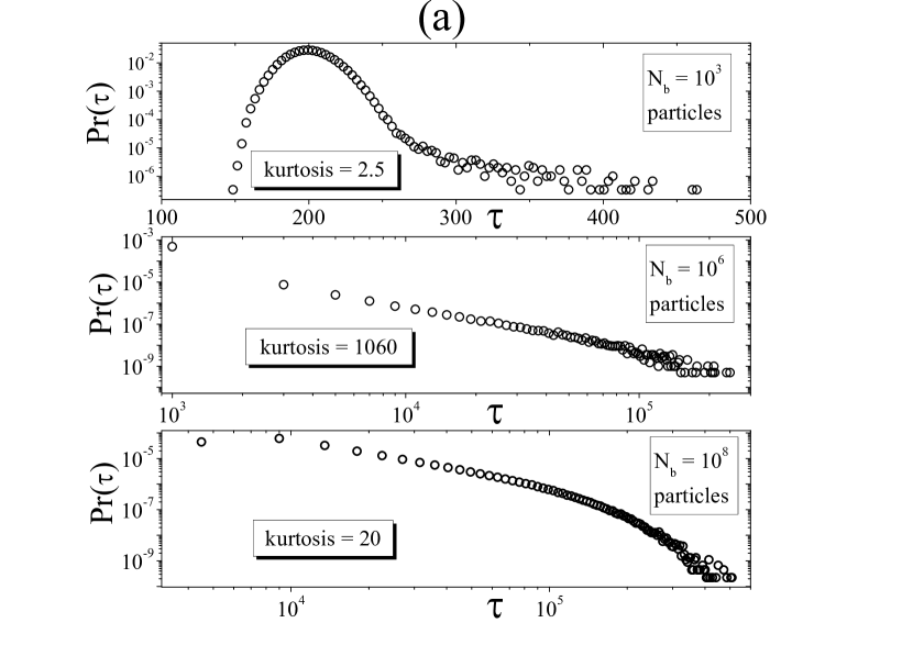
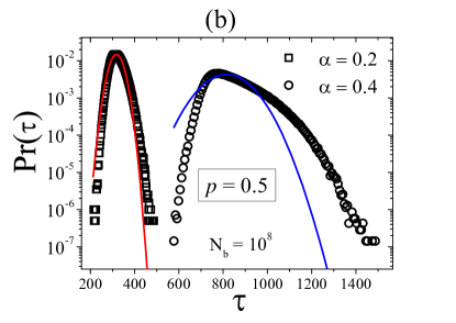
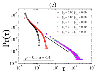
Figure 2: MC simulations for the crossing time distribution. In all tested situations, we used $p=0.5$ and $N_{A}=10^{6}$ particles. Plot (a) shows the effects of the concentration of particles of the species $B$. From the top to the bottom, we have used $N_{B}=10^{3}$, $10^{6}$, and $10^{8}$, respectively. In these three situations, we kept $\alpha=0.4$, $\beta_{\parallel}=0.1$, and $\beta_{\perp}=0$. Plot (b) shows the effects of different values of $\alpha$. Here we also kept $N_{B}=10^{8}$ and $\beta_{\parallel}=\beta_{\perp}=0$. Plot (c) shows two effects obtained by considering different values of $\beta_{\parallel}$ for the same $\beta_{\perp}$ and different values of $\beta_{\perp}$ for the same $\beta_{\parallel}$.

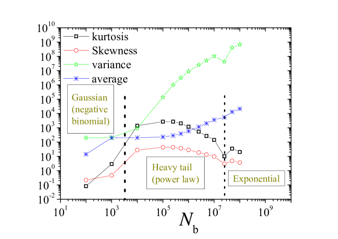
Figure 3: Average, variance, skewness, and kurtosis of the crossing time distribution as function of $N_{B}$. By looking at kurtosis (weight tail) of distribution, we can observe a crossover: Gaussian behavior $\rightarrow$ power law behavior $\rightarrow$ exponential behavior.

Some stylized facts can be observed in Fig. 2, which shows results from MC simulations for the crossing time distribution. In all situations, we used $p=0.5$ and $N_{A}=10^{6}$ particles. Figure 2 (a) shows the effects of different concentrations of particles of the species $B$. From the top to the bottom, we present the plots with $N_{B}=10^{3}$, $10^{6}$, and $10^{8}$, respectively. In these three situations, we used $\alpha=0.4$, $\beta_{\parallel}=0.1$ and $\beta_{\perp}=0$. We measured the kurtosis of distribution for each case, calculated as $\left\langle\left(\frac{\tau-\left\langle\tau\right\rangle}{\delta}\right)^{4}\right\rangle$which measures the weight of tail of crossing time distribution. Here $\left\langle\tau^{k}\right\rangle=\sum_{\tau}\tau^{k}f(\tau)/$ $\sum f(\tau)$, where $f(\tau)$ is the frequency count of crossing times. Here $\delta=$ $\sqrt{\left\langle\tau^{2}\right\rangle-\left\langle\tau\right\rangle^{2}}$ is the standard deviation of crossing time distribution.

Figure 2 (b) shows the effects when different values of $\alpha$ are considered. Here, we kept $N_{B}=10^{8}$ and $\beta_{\parallel}=\beta_{\perp}=0$. We can observe that for $\alpha=0.4$ the deviation of a Gaussian fit (continuous curve) is easily observed. Finally, our the plot (c) in Fig. 2 shows two different effects: different values of $\beta_{\parallel}$ for the same $\beta_{\perp}$ and different values of $\beta_{\perp}$ for the same $\beta_{\parallel}$. It is important to observe that for fixed obstacles, we cannot observe a strong influence of $\beta_{\perp}$ on the crossing times, i.e., the lateral motion is not important since the particles that move laterally (changing lanes) end up encountering other obstacles whereas they are uniformely distributed in the lattice. Different results are obtained when one takes into account an lattice without obstacles, i.e., when both species of particles are able to move in opposite directions.

Let us return to Fig. 2 (a) in order to look into some important details. There is an interesting crossover for the crossing time distribution as function of $N_{B}$. We have a small kurtosis for the top plot ($\sim 2.5$), a large kurtosis for the middle plot ($\sim 1060$), and an intermediate kurtosis for the bottom plot ($\sim 20$). Although it is very interesting, this transition has a simple explanation: for low values of $N_{B}$, one have, in first approximation, a negative binomial distribution (a Gaussian distribution at the limit) with a scattering in the tail since there is no influence of obstacles and the particles have to perform $L_{x}$ movements with $L_{x}/p$ trials until complete the path. When one have an intermediate value of $N_{B}$, an interesting phenomena arises: although there is a more probable crossing time, torn particles are blocked by obstacles since our model is based on relative density and therefore, clusters composed by particles of the same species have a better confront against the particles of the other species. These torn particles correspond to Levy flights since they have huge crossing times when compared with the other ones. Finally, when $N_{B}$ is very large, all particles have a hard task to cross the corridor and, differently from intermediate situation, there is no very different crossing times leading to an exponential behavior.

These crossovers among Gaussian, power law, and exponential behaviors are shown in Fig. 3 through the analysis of the average, variance, kurtosis, and skewness as function of $N_{B}$. As it can be seen, while the average and variance have a monotonic behavior, the kurtosis and skewness have at first an increase and then they decrease corroborating the crossover.

4 Results II: species B in motion - Annealed scenario

Now, we consider that the particles of the species $B$ are also able to move. Firstly, we analyze the fluctuations of spatial particle distribution by considering two opposite streams of particles starting as two stripes at the ends of the corridor (next subsection). Right after, in the second subsection we consider the two different species randomly distributed and mixed in the corridor and we analyze the fluctuations on the distillation time, i.e., the needed time to separate the two species.

4.1 Properties of the spatial particle distribution

As we have already explored the effects of crossing times of particles of the species $A$ when particles of the species $B$ work as fixed obstacles, now we would like to study some effects when the particles of the species $B$ are able to move in the lattice. For this purpose, we analyze the properties of a scenario where two streams of different species of particles interact with each other when moving in opposite direction. So, we consider the condition previously set up to the particles of the species $A$ as valid for both species. The condition for the species $B$ is then given by:

$$n_{B}(j,k;t=0)=\left\{\begin{array}[]{lll}\frac{N_{B}}{L_{y}}&\text{if}&\begin{array}[]{l}j=L_{x},\\ k=1,\cdots,L_{y}\end{array}\\ &&\\ 0&\text{if}&\begin{array}[]{l}1<j<L_{x}-1,\\ k=1,\cdots,L_{y}\end{array}\end{array}\right.$$

Here, we are interested in the study of the scenario when the two species meet each other and interact by following the dynamics previously defined in this work. After starting the evolution of the two stripes, we follow the time evolution of the shape of the density of particles for several times as can be seen in Fig. 4 (a) as well as of the time evolution of the parameters which describe such density, i.e., its fluctuations (plot (b), in the same figure).

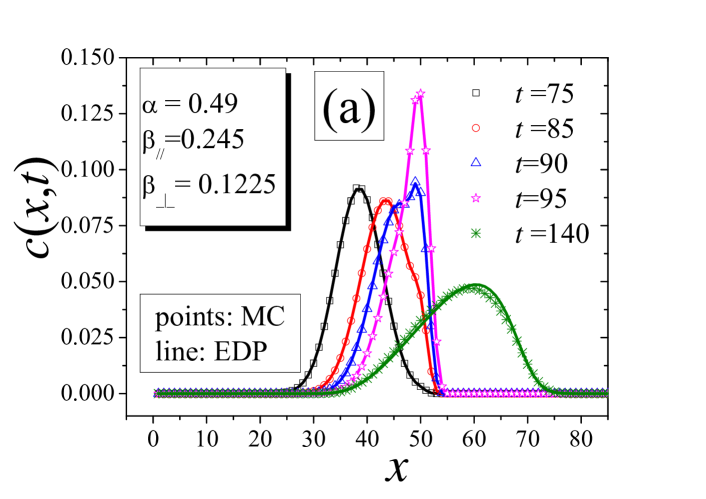
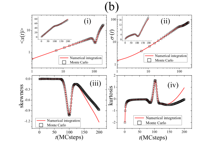
Figure 4: Plot (a): Density of particles $A$ ($B$ is symmetric since the initial conditions are similar) in different times of evolution. Plot (b): Time evolution of fluctuations of the density of particles: average, standard deviation, skewness and kurtosis.

We can observe in Fig. 4 (a) that the density of particles $c(x,t)$ (at cell $j=x/a$ and time $t=l\Delta$) is deformed during the interaction of the species from $t=85$. Here it is important to notice that a marginalization over $y$ dimension was conveniently performed according to our objectives. Figure 4 (b) shows that this deformation is captured by valleys in the skewness (iii):$\ \left[\sum_{x}\left(\frac{x-\left\langle x(t)\right\rangle}{\sigma(t)}\right)^{3}c(x,t)\right]/\sum_{x}c(x,t)$ and peaks in the kurtosis (iv): $\left[\sum_{x}\left(\frac{x-\left\langle x(t)\right\rangle}{\sigma(t)}\right)^{4}c(x,t)\right]/\sum_{x}c(x,t)$, with $\left\langle x(t)\right\rangle=\left[\sum_{x}xc(x,t)\right]/\sum_{x}c(x,t)$ and $\sigma(t)=\left[\left\langle x^{2}(t)\right\rangle-\left\langle x(t)\right\rangle^{2}\right]^{1/2}$, that increase in absolute value during the evolution, leaving the Gaussian behavior (represented by the distribution for $t=75$ as showed in plot (a)) to become a heavy tail distribution. We also can observe that such anomalous behavior is also captured by the average position $\left\langle x(t)\right\rangle$, in the plot (i) as well as by the standard deviation of the position $\sigma(t)$ of the particles according to plot (ii). In both plots we use $\alpha=0.49$, $\beta_{\parallel}=0.245$ and $\beta_{\perp}=0.1225$. In Fig. 4 (a) and (b) we also present the comparison between the results obtained through MC simulations and EDP solutions. As shown, they are in good agreement to each other.

4.2 Distillation time

As the two species of particles follow opposite directions, an interesting situation can be observed when we mix them in the corridor at the initial stage of the evolution and analyze the needed time to a complete separation of the two species (distillation). In Fig. 5 we show a typical situation in which the species are completed distillate.

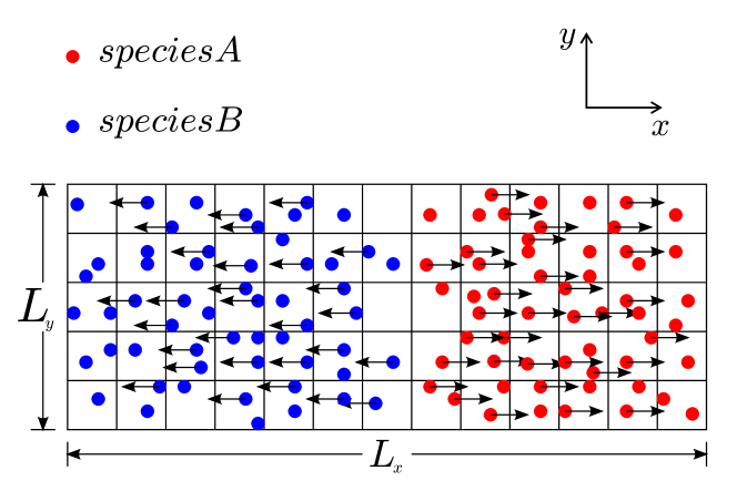
Figure 5: Illustration of a complete distillation between the species $A$ and $B$. This means that there is a vertical line separating the two species in the corridor.

The needed time for the system to achieve the complete separation of the species is computed through numerical MC simulations for all possible pairs $\left(\beta_{\parallel},\beta_{\perp}\right)$ for two different values of $\alpha$, one low: 0.1, and another high: 0.4. This procedure was repeated considering three different number of particles $N=N_{A}=N_{B}=100$, 500, and 1000. Here, the main idea is to check if $\beta_{\perp}$ can affect the distillation time. Figure 6 shows that for $\alpha=0.1$ the effects of $\beta_{\perp}$ on the distillation time are not perceptible, however $\alpha=0.4$ leads to a reduction of the distillation time.

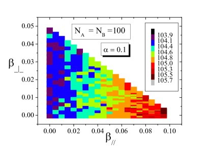
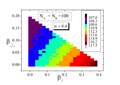
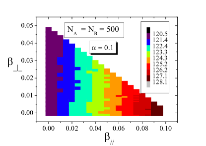
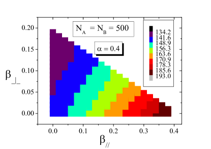
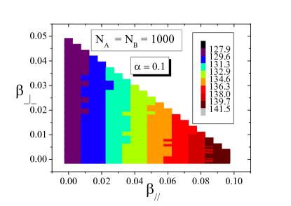
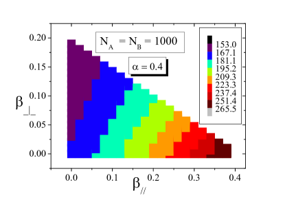
Figure 6: Color map of the distillation time for different values of $\beta_{\parallel}$ and $\beta_{\perp}$ considering different concentrations of particles for two different values of $\alpha$.

This reduction is more relevant when $\beta_{\parallel}$ is higher, i.e., the movements to the sides are important when the combination of the resistance factor ($\alpha$) and the frontal collision effects ($\beta_{\parallel}$) leads to a real stagnation in the movement ability. Here, it is interesting to monitor the order parameters $\Phi_{cell}(t)$ and $\Phi_{\perp}(t)$ as function of time during the distillation previously described in Fig. 6. We hope that when $t\rightarrow\infty$, both $\Phi_{cell}$ and $\Phi_{\perp}\rightarrow 1$ since the system is completely distillate.

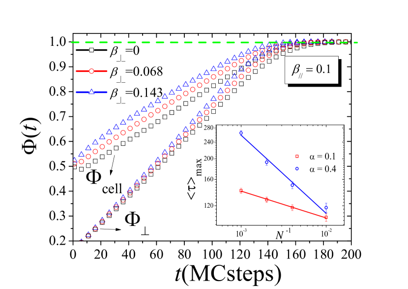
Figure 7: Time evolution of the order parameters $\Phi_{cell}$ and $\Phi_{\perp}$ for $\beta_{\parallel}$ fixed and for different values of $\beta_{\perp}$. We can observe that both parameters converge to 1 (indicating that the system is completely distillate), and the segregation is greater as $\beta_{\perp}$ increases. The inset plot shows as the distillation times scales with the number of particles.

In Fig. 7 we show that both parameters converge to 1 (indicating that the system is completely distillate), and the segregation is greater as $\beta_{\perp}$ increases. A simple analysis of the finite size scaling effects of the average time of the distillation time is shown in the inset of this figure. This plot is obtained for the worst case ($\beta_{\perp}=0$ and the maximal allowed $\beta_{\parallel}$, i.e., $\beta_{\parallel}=\alpha$) as function of the inverse number of particles in the system: $N^{-1}=N_{A}^{-1}=N_{B}^{-1}$, and is presented in log-log scale for the two studied values of $\alpha$.

Whereas we have already explored the properties of the distillation time and the dependence of the different factors that change this quantity, we study, in the following section, the band formation which appears when the particles move in a ring which is obtained by considering periodic boundary conditions in the longitudinal direction.

5 Results III: Periodic boundary conditions - motion in a ring

Now, we consider the two species of particles moving in a ring, in the opposite direction to each other, i.e., one species of particles is moving in the counterclockwise and the another one is moving in the clockwise. Alternatively, this situation can be thought as if particles could enter in the corridor according to some rate if they are of the same species that those which are reaching the end of corridor (ring topology). The idea is represented in Fig. 8.

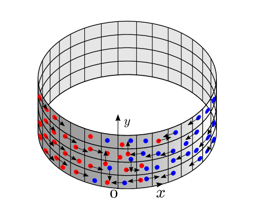
Figure 8: Particle counterflow of different species moving in a ring.

First of all, we perform MC simulations considering that the species have the same number of particles ($N_{A}=N_{B}=10^{5}$) and are uniformily distributed in the corridor. Thus, we monitor the concentrations of particles in the corridor as the time evolves, for a typical set of parameters $\alpha=0.45$ and $\beta_{\parallel}=\beta_{\perp}=0.15$ in order to observe the process of relaxation toward the formation of bands. We analyze the frames for three different MC steps: $t=1$, $1100$, and $64000$. Band formations can be observed after a long time corroborating the ordering of the species which move in the same direction in the stationary stage of the evolution.

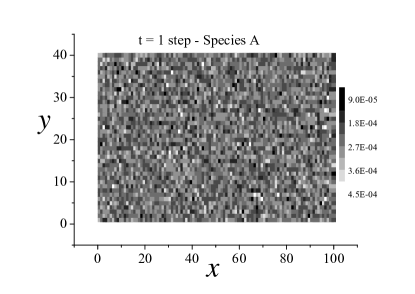
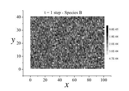
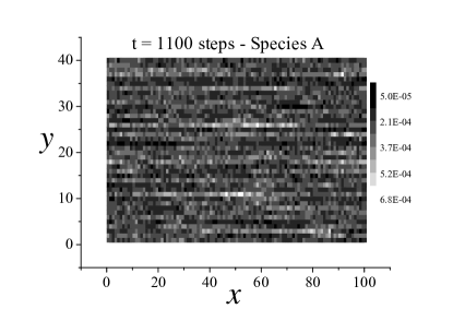
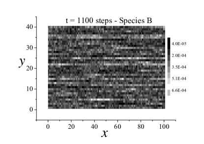
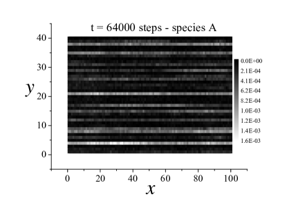
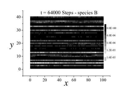
Figure 9: Frames of the density of particles of the species $A$ (left side) and $B$ (right side) for different instants of time when the species move in opposite direction. The particles are uniformily distributed at the beginning of the evolution and follow the ring topology. Band formations can be observed in the final of evolution.

Such patterns can be better understood if we analyze the order parameters $\Phi_{\parallel}(t)$, $\Phi_{cell}(t)$, and $\Phi_{\perp}(t)$ as function of the time. We can observe in Fig. 10 that $\Phi_{\parallel}(t)$ goes asymptotically to 1, which corroborates the longitudinal bands observed in Fig. 9. Likewise, we can see that $\Phi_{cell}(t)$ converges to 1 since a segregation by bands (longitudinal or vertical) implies in a segregation by cells. However, $\Phi_{\perp}(t)$ possesses lower values showing that the segregation by vertical bands (perpendicular to the orientation field of particles) is not expected.

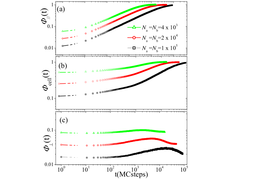
Figure 10: Relaxation of the order parameters. We can see that $\Phi_{\parallel}$ and $\Phi_{cell}$ go to 1 when $t\rightarrow\infty$ corroborating the ordering of the species in longitudinal bands. However the segregation by bands in the perpendicular direction to the field is not observed.

Here, it is interesting to make an analogy with some real physical systems. Vissers et al. [16] observed an interesting lane formation in driven mixtures of oppositely charged colloids when considering periodic boundary conditions and their results corroborate our theoretical findings in a purely stochastic model (see Fig. 1 in Ref. [16]). In other publication, Vissers et al. [17] showed that vertical bands appear when one apply an ac field. In a upcoming paper, we will explore the effects due to an ac field in a stochastic model in order to reproduce such experimental results.

In a recent work, Oliveira et al. [7] proposed a model of pedestrian behavior and obtained two-lane ordered state emerging with asymmetrically shaped walls. So, they were are able to organize the flow of pedestrians moving in opposite directions by solving Langevin-like equations with Stokesian drag force. Inspired in this work, we propose an interesting computational experiment by using our model. However, differently from that study, we focus our attention to initial conditions of the particles. So, we start with the particles of the species $A$ initially concentrated in a vertical stripe asymmetrically distributed along $y$:

$$n_{A}(j,k;t=0)=\left\{\begin{array}[]{lll}\frac{2N_{A}}{L_{y}}(L_{y}-k)&\text{if}&j=1,k=1,\cdots,L_{y}\\ &&\\ 0&\text{if}&\begin{array}[]{l}2\leq j\leq L_{x},\\ k=1,\cdots,L_{y}\end{array}\end{array}\right.$$ (7)

and the particles of the species $B$ are uniformly distributed on the corridor: $n_{B}(j,k;t=0)=N_{B}/(L_{x}L_{y})$, with $j=1,\cdots,L_{x}$ and $k=1,\cdots,L_{y}$. The highlight here is the possibility of obtaining a stationary state with two-lane ordered state if initial condition defined above is capable to induce such similar stationary state in $B$. We solve the problem using MC simulations and numerical integration of Eq. (2) to compare the stages of evolution. In Fig. 11, we show the frames for six different instants of time. The blue (red) color means higher (lower) concentrations of a given species.

where these figures blue means more concentrated while red less concentrated

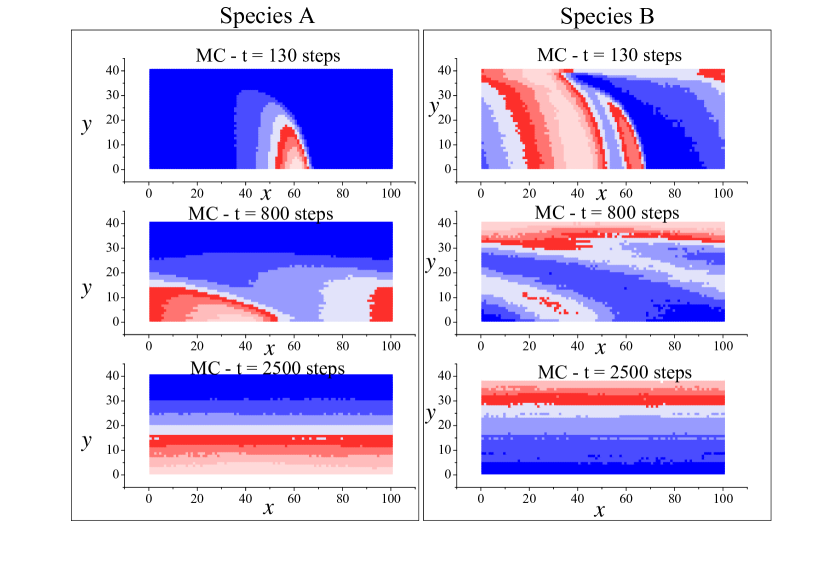
Figure 11: Frames of some instants of time using MC simulations. We can observe stationary states with two well distinct emergent ordered lanes . The blue (red) color means higher concentrations of the species $A$ ($B$) in the plots of the left (right). An assimetry is initially considered for species $A$ according to Eq. (7) while the species $B$ is uniformly distributed.

We can observe that even with an asymmetric initial condition, the system has the tendency to reach a stationary order formed by two ordered lanes differently of what happens when one considers initial conditions where the particles of both species are uniformly distributed. Figure 12 shows the frames for the same instants of time when one takes into consideration the numerical integration of Eq. (2). Both methods lead to stationary states with two emergent ordered lanes. It is important to observe that numerical integration of equations corresponds to the mean field regime of MC simulations and, although we have similar evolution and the same stationary state, the relaxations are not synchronized. This is exactly what should occur in Statistical Mechanics when, for example, we solve the Ising model by performing MC simulations and via Mean-field approach. In these cases, the critical exponents associated to possible phase transitions are different. However, we expect that $\Phi_{\parallel}\rightarrow 1$ in both cases even though with different speeds since Figs. 11 and 12 present different time scales of relaxation dynamics.

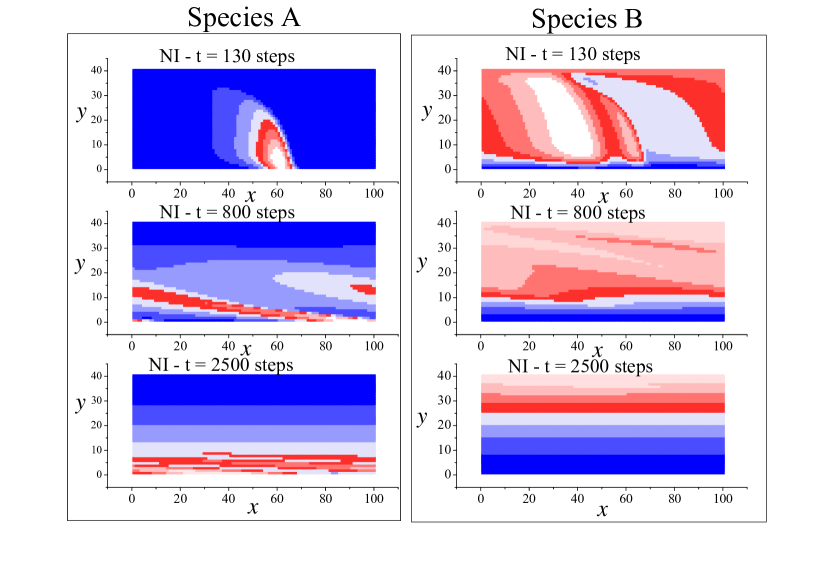
Figure 12: Frames obtained via numerical integration of recurrence relations for six different instants of time (as in Fig. 11). The blue (red) color means higher concentrations of the species $A$ ($B$) in the plots of the left (right). An assimetry is initially considered for species $A$ according to Eq. (7) while the species $B$ is uniformly distributed.

Figure 13 shows the time evolution of the three order parameters of the model. These evolutions are obtained when carrying out the study corresponding to the Fig. 11 (MC simulations) and Fig. 12 (NI).

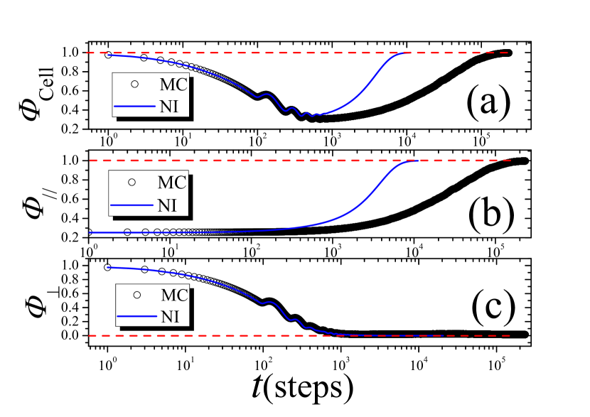
Figure 13: Time evolution of the order parameters considering that the species $A$ is asymmetrically distributed in an inital vertical stripe according to Eq. (7) and the species $B$ is uniformily distributed in the lattice. Both methods (MC simulations and NI) lead to stationary states as previously shown in Figs. 11 and 12 composed by two emergent ordered bands which are quantitatively corroborated by the order parameters $\Phi_{cell}\rightarrow 1$ (a) and $\Phi_{\parallel}\rightarrow 1$ (b), when $t\rightarrow\infty$. We also show the behavior of $\Phi_{\perp}$ as function of time. In this case $\Phi_{\perp}\rightarrow 0$ since the particles do not present order by bands perpendicular to the field.

We can observe in Fig. 13 that $\Phi_{cell}\rightarrow 1$ and $\Phi_{\parallel}\rightarrow 1$ (using MC simulations and also NI) show the stationary case formed by two main bands corresponding to the two species. The observed difference in the plots are acceptable since we do not expect the same speed in the two solutions but instead we expect the reproduction of the same steady states. However it is important to observe that the initial part is exactly the same for all order parameters and only the conduction to the steady state is slower for the MC simulations. Such problem shows a interesting situation where an initial order of species $A$ is broken after a transient regime reaches an ordered dynamics.

6 Summary and conclusions

We have considered a two-dimensional system composed by particles of two species, $A$ and $B$, which are able to move or not. If one of the species remains still, it acts as fixed obstacles to the other species which is moving. In this case, we used MC simulations and concentrated our analysis in the statistics about crossing times (which means the needed time for one particle cross the lattice) for different concentrations of obstacles. However, if both species are moving, then they move in opposite diretions. In this case, we looked into the properties of distillation times of the particles arranged randomly in the lattice at the beginning of the evolution, as well as the formation of ordering patterns considering periodic boundary conditions of particles. Both studies were performed by using MC simulations and numerical integration of recurrence relations. In the first study, we showed that an interesting transition between the Gaussian, power law, and exponential behavior is observed for the crossing times of the particles, which is supported by high kurtosis values. We also showed that the correlation times are not affected by lateral transitions. In the second study, when both species can move, we observed that the enlarge of lateral transitions decreases the distillation times and the particles are more easily separated.

Finally, we observed characteristic ordering patterns, which appear also in charged colloids motions and pedestrian dynamics, when our two-dimensional model took into consideration periodic boundary conditions. It is important to notice that Dickman [20] has observed that similar spontaneous spatial ordering, which appears in systems of self-propelled agents, can also appear in driven lattice-gas. In this case, it was found an interesting phenomena where the drive can provoke jamming, and thereby, a sharp reduction in the current, quite contrary to the usual relation between bias and current. As future works, we will explore exclusion effects, for example by introducing in our model, cells with limited maximum number of particles and analyse these effects into ordering formation.

Acknowledgments – This research work was in part supported financially by CNPq (National Council for Scientific and Technological Development).

References

- [1] S. Machlup, J. Appl. Phys, 35, 341(1954).
- [2] M.J. Kirton, M.J. Uren Adv. Phys., 38, 367(1989)
- [3] R. da Silva, L. C. Lamb, G. I. Wirth, Philos. T. Roy. Soc. A, 369, 307-321(2011), R. da Silva, L. Brusamarello, G. Wirth, Physica. A 389, 2687-2699 (2010), R. da Silva, G. I. Wirth, J. Stat. Mech., P04025 (2010), R. da Silva, G. I. Wirth, L. Brusamarello, Int. J. Mod. Phys. B, 24, 5885 (2010), R. da Silva, G. I. Wirth, L. Brusamarello, J. Stat. Mech., P10015 (2008).
- [4] S.P. Gross, Phys. Biol. 1, R1–R11 (2004), L. W. Rossi, P. K. Radtke, C. Goldman, Physica. A, 401, 319-329 (2014), C. Goldman, J. Stat. Phys. 140, 1167–1181(2010)
- [5] J.C. Giddings, H. Eyring, J. Phys. Chem., 59, 416 (1955), R. da Silva, L. C. Lamb, E. C. Lima, J. Dupont, Physica. A, 391, 1-7(2012).
- [6] Y. Li, X. Li, Y. Wang, Y.Yin Chen, J. Ji, Y. Yu, and Z. Xu, Ind. Eng. Chem. Res., 53 4821 (2014)
- [7] C. L. N. Oliveira, A. P. Vieira, D. Helbing, J. S. Andrade Jr., H. J. Herrmann, Phys. Rev. X, 6 011003 (2016)
- [8] Xiong T, Zhang P, Wong S C, Shu C W, Zhang M P, Chin. Phys. Lett., 28 108901 (2011)
- [9] L. Xiang, D. Xiao-Yin, D. Li-Yun, Chin. Phys. Lett., 21 108901 (2012)
- [10] T. Kretz, A. GrÃnebohm, M. Kaufman, F. Mazur, M. Schreckenberg, J.Stat.Mech. (2006) P10001
- [11] D. Helbing, I. J. Farkas, T. Vicsek, Nature 407, 487 (2000)
- [12] D. Helbing, P. Molnár, Phys. Rev. E 51 4282 (1995)
- [13] P. Gawronski, K. Kułakowski, Comp. Phys. Comm. 182, 1924–1927 (2011)
- [14] Yu-Cih Peng, Chung-I Chou, Comp. Phys. Comm. 182 205–208 (2011)
- [15] A. Nakayama, K. Hasebe , Y. Sugiyama, 177, 162–163 (2007)
- [16] T. Vussers, A. Wysocki, M. Rex, H. Lowen, C. P. Royall, A. Imhof, A. van Blaaderen, Soft Matter, 7, 2352 (2011)
- [17] T. Vissers, A. van Blaaderen, A. Imnhof, Phys. Rev. Lett. 106, 228303 (2011)
- [18] R. da Silva, A. Hentz; A. Alves, Physica A, 437 139 (2015)
- [19] E. W. Montroll, B. West, On Enriched Collection of Stochastic Process: in Fluctuation Phenomena, Eds. E. W. Montroll and J. Lebowitz (1979)
- [20] R. Dickman, Phys. Rev. E, 64, 016124 (2001)