Performance Impact of Base Station
Antenna Heights in Dense Cellular Networks

Abstract

In this paper, we present a new and significant theoretical discovery. If the absolute height difference between base station (BS) antenna and user equipment (UE) antenna is larger than zero, then the network performance in terms of both the coverage probability and the area spectral efficiency (ASE) will continuously decrease toward zero as the BS density increases in ultra-dense networks (UDNs). Such findings are completely different from the conclusions in existing works, both quantitatively and qualitatively. In particular, this performance behavior has a tremendous impact on the deployment of the 5th-generation (5G) UDNs. Network operators may invest large amounts of money in deploying more network infrastructure to only obtain an even less network capacity. Our study results reveal that one way to address this issue is to lower the BS antenna height to the UE antenna height. However, this requires a revolutionized approach of BS architecture and deployment, which is explored in this paper too.

I Introduction

From 1950 to 2000, the wireless network capacity has increased around 1 million fold, in which an astounding 2700× gain was achieved through network densification using smaller cells [1]. In the first decade of 2000, network densification continued to fuel the 3rd Generation Partnership Project (3GPP) 4th-generation (4G) Long Term Evolution (LTE) networks, and is expected to remain as one of the main forces to drive the 5th-generation (5G) networks onward [2]. Indeed, the orthogonal deployment of ultra-dense (UD) small cell networks (SCNs) within the existing macrocell network, i.e., small cells and macrocells operating on different frequency spectrum (3GPP Small Cell Scenario #2a [3]), is envisaged as the workhorse for capacity enhancement in 5G due to its large spectrum reuse and its easy management; the latter one arising from its low interaction with the macrocell tier, e.g., no inter-tier interference [2]. In this paper, the focus is on the analysis of these UD SCNs with an orthogonal deployment with the macrocells.

Before 2015, the common understanding on ultra-dense networks (UDNs) was that the density of base stations (BSs) would not affect the per-BS coverage probability performance in interference-limited and fully-loaded wireless networks, and thus the area spectral efficiency (ASE) performance in $\textrm{bps/Hz/km}^{2}$ would scale linearly with the network densification [4]. The implication of such conclusion is huge: The BS density does NOT matter, since the increase in the interference power caused by a denser network would be exactly compensated by the increase in the signal power due to the reduced distance between transmitters and receivers. Hence, we do not need to worry about the quantity of the interferers in UDNs because the signal power can always maintain a superior quality over the aggregate interference power with the network densification. Fig. 1 shows the theoretical ASE performance predicted in [4] across the typical BS density regions for various generations of telecommunication systems.

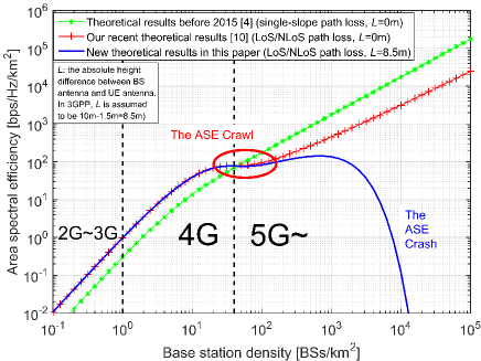
Fig. 1: Theoretical comparison of the ASE performance in $\textrm{bps/Hz/km}^{2}$. Note that all the results are obtained using practical 3GPP channel models [5, 6], which will be introduced later.

However, it is important to note that this conclusion in [4] was obtained with considerable simplifications on the propagation environment, which should be placed under scrutiny when evaluating UDNs, since they are fundamentally different from sparse ones in various aspects [2].

In the past year, a few noteworthy studies have been carried out to revisit the network performance analysis for UDNs under more practical propagation assumptions. In [7], the authors considered a multi-slope piece-wise path loss function, while in [8], the authors investigated line-of-sight (LoS) and non-line-of-sight (NLoS) transmission as a probabilistic event for a millimeter wave communication scenario. The most important finding in these two works was that the per-BS coverage probability performance starts to decrease when the BS density is sufficiently large. Fortunately, such decrease of coverage probability will not change the monotonic increase of the ASE as the BS density increases [7, 8].

In our very recent work [9, 10], we took a step further and generalized the works in [7, 8] by considering both piece-wise path loss functions and probabilistic LoS/NLoS transmissions. We found that the ASE will suffer from a slow growth or even a small decrease on the journey from 4G to 5G when the BS density is larger than a threshold. Fig. 1 shows such theoretical results on the ASE performance, where such threshold is around 20 $\textrm{BSs/km}^{2}$ and the slow/negative ASE growth is highlighted by a circled area. This circled area is referred to as the ASE Crawl hereafter. The intuition of the ASE Crawl is that the aggregate interference power increases faster than the signal power due to the transition of a large number of interference paths from NLoS to LoS with the network densification. The implication is profound: The BS density DOES matter, since it affects the signal to interference relationship in terms of the power ratio. Hence, in UDNs we need to pay special attention to the quality of the interferers, because many of them may transit from NLoS to LoS, thus overwhelming the useful signal. As a result, network operators should be careful when deploying dense SCNs in order to avoid investing huge amounts of money and end up obtaining no performance gain due to the ASE Crawl. Fortunately, our results in [9, 10] also pointed out that the ASE will again grow almost linearly as the network further evolves to a UDN, e.g., $>10^{3}\thinspace\textrm{BSs/km}^{2}$ in Fig. 1. According to our results and considering a 300 MHz bandwidth, if the BS density can go as high as $10^{4}\thinspace\textrm{BSs/km}^{2}$, the problem of the ASE Crawl caused by the NLoS to LoS transition of interfering paths can be overcome, and an area throughput of $10^{3}\thinspace\textrm{Gbps/km}^{2}$ can be achieved, thus opening up an efficient way forward to 5G.

Unfortunately, the NLoS to LoS transition of interference paths is not the only obstacle to efficient UDNs in 5G, and there are more challenges to overcome to get there. In this paper, we present a serious problem posed by the absolute antenna height difference between BSs and user equipments (UEs), and evaluate its impact on UDNs by means of a three-dimensional (3D) stochastic geometry analysis (SGA). We made a new and significant theoretical discovery: If the absolute antenna height difference between BSs and UEs, denoted by $L$, is larger than zero, then the ASE performance will continuously decrease toward zero as the network goes ultra-dense. Fig. 1 illustrates the significance of such theoretical finding with $L=8.5$ m: After the ASE Crawl, the ASE performance only increases marginally (~1.4x) from 109.1 $\textrm{bps/Hz/km}^{2}$ to 149.6 $\textrm{bps/Hz/km}^{2}$ as the BS density goes from $200\thinspace\textrm{BSs/km}^{2}$ to $10^{3}\thinspace\textrm{BSs/km}^{2}$, which is then followed by a continuous and quick fall to zero starting from around $10^{3}\thinspace\textrm{BSs/km}^{2}$. The implication of this result is even more profound than that of the ASE Crawl, since following a traditional deployment with BSs deployed at lamp posts or similar heights will dramatically reduce the network performance in 5G. Such decline of ASE in UDNs will be referred to as the ASE Crash hereafter, and its fundamental reasons will be explained in detail later in this paper.

In order to address the problem of the ASE Crash, we propose to change the traditional BS deployment, and lower the BS antenna height, not just by a few meters, but straight to the UE antenna height [12], so that the ASE behavior of UDNs can roll back to our previous results in [10], thus avoiding the ASE Crash. However, this brings revolutionized BS deployments and new hardware issues, which will be discussed later.

The rest of this paper is structured as follows. Section II provides a brief review on the related work. Section III describes the system model for the 3D SGA. Section IV presents our theoretical results on the coverage probability and the ASE performance. The numerical results are discussed in Section V, with remarks shedding new light on the ASE Crash phenomenon. Finally, the conclusions are drawn in Section VI.

II Related Work

In stochastic geometry, BS positions are typically modeled as a Homogeneous Poisson Point Process (HPPP) on the plane, and closed-form expressions of coverage probability can be found for some scenarios in single-tier cellular networks [4] and multi-tier cellular networks [13]. The major conclusion in [4, 13] is that neither the number of cells nor the number of cell tiers changes the coverage probability in interference-limited fully-loaded wireless networks. Recently, a few noteworthy studies have been carried out to revisit the network performance analysis for dense and UDNs under more practical propagation assumptions. As have discussed in Section I, the authors of [7] and [8] found that the per-BS coverage probability performance will start to decrease when the BS density is sufficiently large. In our very recent work [9, 10], we presented a new finding that the ASE will suffer from a slow growth or even a small decrease on the journey from 4G to 5G when the BS density is larger than a threshold, i.e., the ASE Crawl. However, none of the above works considered the antenna heights of BSs and UEs in the theoretical analysis, which will be the focus of this work. It is very important to note that the authors of [14, 15] recently proposed a new approach of network performance analysis based on HPPP intensity matching. Such new approach may also be used to investigate the BS antenna height issue, and it is interesting to conduct a comparison study on the intensity matching approach and our analysis in terms of the accuracy loss due to approximation and the computational complexity, etc. In this work, we will focus on revealing the ASE Crash phenomenon using the traditional framework developed in [7, 8, 9, 10].

Another research area relating to the antenna height issue is that of unmanned aerial vehicles (UAVs), which has attracted significant attention as key enablers for rapid network deployment, where the antenna heights of drone BSs and ground UEs are usually considered [16, 17, 18, 19]. Generally speaking, the works on drone BSs put a lot of emphasis on the 3D mobility of UAVs and try to numerically find the optimal position/height for the drone deployment in a small area involving just one or a few flying BSs. In contrast, our work considers a large-scale, randomly-deployed and stationary cellular network, paying special attention to the capacity scaling law of the whole network.

III System Model

We consider a downlink (DL) cellular network with BSs deployed on a plane according to a homogeneous Poisson point process (HPPP) $\Phi$ with a density of $\lambda$ $\textrm{BSs/km}^{2}$. Note that the value of $\lambda$ is in the order of 10~100 for the current 4G networks [5]. UEs are Poisson distributed in the considered network with a density of $\rho$ $\textrm{UEs/km}^{2}$. Note that $\rho$ is assumed to be sufficiently larger than $\lambda$ so that each BS has at least one associated UE in its coverage [7, 8, 9, 10]. The two-dimensional (2D) distance between a BS and a UE is denoted by $r$. Moreover, the absolute antenna height difference between a BS and a UE is denoted by $L$. Note that the value of $L$ is in the order of several meters. As discussed in Section I, for the current 4G networks, $L$ is around 8.5 m because the BS antenna height and the UE antenna height are assumed to be 10 m and 1.5 m, respectively [11]. Hence, the 3D distance between a BS and a UE can be expressed as

$$w=\sqrt{r^{2}+L^{2}}.$$ (1)

Note that an alternative method is to present the 3D distance in polar coordinates as in [20].

Following [9, 10], we adopt a very general path loss model, in which the path loss $\zeta\left(w\right)$ associated with distance $w$ is segmented into $N$ pieces written as

$$\zeta\left(w\right)=\begin{cases}\zeta_{1}\left(w\right),&\textrm{when }L\leq w\leq d_{1}\\ \zeta_{2}\left(w\right),&\textrm{when }d_{1}<w\leq d_{2}\\ \vdots&\vdots\\ \zeta_{N}\left(w\right),&\textrm{when }w>d_{N-1}\end{cases},$$ (2)

where each piece $\zeta_{n}\left(w\right),n\in\left\{1,2,\ldots,N\right\}$ is modeled as

$$\zeta_{n}\left(w\right)=\begin{cases}\begin{array}[]{l}\zeta_{n}^{\textrm{L}}\left(w\right)=A_{n}^{{\rm{L}}}w^{-\alpha_{n}^{{\rm{L}}}},\\ \zeta_{n}^{\textrm{NL}}\left(w\right)=A_{n}^{{\rm{NL}}}w^{-\alpha_{n}^{{\rm{NL}}}},\end{array}&\begin{array}[]{l}\textrm{LoS:}\leavevmode\nobreak\ \textrm{Pr}_{n}^{\textrm{L}}\left(w\right)\\ \textrm{NLoS:}\leavevmode\nobreak\ 1-\textrm{Pr}_{n}^{\textrm{L}}\left(w\right)\end{array},\end{cases}$$ (3)

where $\zeta_{n}^{\textrm{L}}\left(w\right)$ and $\zeta_{n}^{\textrm{NL}}\left(w\right),n\in\left\{1,2,\ldots,N\right\}$ are the $n$-th piece path loss functions for the LoS transmission and the NLoS transmission, respectively, $A_{n}^{{\rm{L}}}$ and $A_{n}^{{\rm{NL}}}$ are the path losses at a reference distance $w=1$ for the LoS and the NLoS cases, respectively, and $\alpha_{n}^{{\rm{L}}}$ and $\alpha_{n}^{{\rm{NL}}}$ are the path loss exponents for the LoS and the NLoS cases, respectively. In practice, $A_{n}^{{\rm{L}}}$, $A_{n}^{{\rm{NL}}}$, $\alpha_{n}^{{\rm{L}}}$ and $\alpha_{n}^{{\rm{NL}}}$ are constants obtainable from field tests [5, 6]. It is very important to note that the values of the above parameters should be chosen to ensure the continuity and the monotonically decreasing property of the path loss function $\zeta\left(w\right)$, as the 3GPP has practiced in [5, 6]. Moreover, $\textrm{Pr}_{n}^{\textrm{L}}\left(w\right)$ is the $n$-th piece LoS probability function that a transmitter and a receiver separated by a distance $w$ has a LoS path, which is assumed to be a monotonically decreasing function with regard to $w$ in this paper.

For convenience, $\left\{\zeta_{n}^{\textrm{L}}\left(w\right)\right\}$ and $\left\{\zeta_{n}^{\textrm{NL}}\left(w\right)\right\}$ are further formulated as piece-wise functions:

$$\zeta^{Path}\left(w\right)=\begin{cases}\zeta_{1}^{Path}\left(w\right),&\textrm{when }L\leq w\leq d_{1}\\ \zeta_{2}^{Path}\left(w\right),&\textrm{when }d_{1}<w\leq d_{2}\\ \vdots&\vdots\\ \zeta_{N}^{Path}\left(w\right),&\textrm{when }w>d_{N-1}\end{cases},$$ (4)

where the string variable $Path$ takes the value of “L” and “NL” for the LoS and the NLoS cases, respectively. Besides, $\left\{\textrm{Pr}_{n}^{\textrm{L}}\left(w\right)\right\}$ is also formulated as a piece-wise function:

$$\textrm{Pr}^{\textrm{L}}\left(w\right)=\begin{cases}\textrm{Pr}_{1}^{\textrm{L}}\left(w\right),&\textrm{when }L\leq w\leq d_{1}\\ \textrm{Pr}_{2}^{\textrm{L}}\left(w\right),&\textrm{when }d_{1}<w\leq d_{2}\\ \vdots&\vdots\\ \textrm{Pr}_{N}^{\textrm{L}}\left(w\right),&\textrm{when }w>d_{N-1}\end{cases}.$$ (5)

The generality and the practicality of the adopted path loss model (2) have been well established in [10]. In particular, note that (2) can be easily degenerated to a simplistic single-slope path loss model as [4]

$$\zeta\left(w\right)=Aw^{-\alpha},$$ (6)

which can be obtained from (3) with $N=1$, $A_{1}^{{\rm{L}}}=A_{1}^{{\rm{NL}}}=A$, $\alpha_{1}^{{\rm{L}}}=\alpha_{1}^{{\rm{NL}}}=\alpha$, and $\textrm{Pr}^{\textrm{L}}\left(w\right)=1$. Consequently, our analytical results to be presented in later sections can be easily applied to such simplistic single-slope path loss model (6) with the above parameter substitution. It should be noted that the adopted path loss model (2) is fundamentally different from the simplistic single-slope path loss model (6). In more detail, for (2), we assume a practical user association strategy (UAS), in which each UE is connected to the BS with the smallest path loss (i.e., with the largest $\zeta\left(w\right)$) [8, 10]. Such assumption reflects the fact that in reality a UE might connect to a BS that is not the nearest one but with a strong LoS path, rather than to the nearest BS with a weak NLoS path. However, for (6), each UE is always associated with the BS at the closest proximity [4].

Moreover, we assume that each BS/UE is equipped with an isotropic antenna, and that the multi-path fading between a BS and a UE is modeled as independently identical distributed (i.i.d.) Rayleigh fading [7, 8, 9, 10]. In order to investigate more realistic channel environments, we further perform the following studies:

• A practical antenna pattern and downtilt will be considered in Subsection V-D with performance evaluated by simulations. Note that in practice each BS antenna has a 3D beam pattern and such beam will be electrically tilted downward to improve the signal power as well as reduce the inter-cell interference [21, 22, 23]. Intuitively speaking, the downtilt angle should increase with the network densification since each BS’s effective coverage area shrinks. For example, the downtilt angle is around 10 degrees for macrocell BSs in [11] and it is significantly larger for small cell BSs [2].

• A practical Rician fading will be analyzed in Subsection IV-D and evaluated in Subsection V-E to show its minor impact on our conclusions.

• Two practical 3GPP path loss models will be introduced as special examples of (2) in Subsection IV-E. These two path loss models as well as the single-slope path loss model (6) will be evaluated in Section V to show the generality of our results.

IV Main Results

Using a 3D SGA based on the HPPP theory, we study the performance of the SCN by considering the performance of a typical UE located at the origin $o$.

IV-A The Coverage Probability

We first investigate the coverage probability $p^{{\rm{cov}}}\left(\lambda,\gamma\right)$ that the typical UE’s signal-to-interference-plus-noise ratio (SINR) is above a per-designated threshold $\gamma$:

$$p^{{\rm{cov}}}\left(\lambda,\gamma\right)=\textrm{Pr}\left[\mathrm{SINR}>\gamma\right],$$ (7)

where the SINR is calculated as

$$\mathrm{SINR}=\frac{P\zeta\left(w\right)h}{I_{{\rm{agg}}}+P_{{\rm{N}}}},$$ (8)

where $h$ is the channel gain, modeled as an exponential random variable (RV) with the mean of one (due to our consideration of Rayleigh fading in this paper), $P$ is the transmission power of each BS, $P_{{\rm{N}}}$ is the additive white Gaussian noise (AWGN) power at each UE, and $I_{{\rm{agg}}}$ is the aggregate interference given by

$$I_{{\rm{agg}}}=\sum_{i:\,b_{i}\in\Phi\setminus b_{o}}P\beta_{i}g_{i},$$ (9)

where $b_{o}$ is the BS serving the typical UE at distance $w$ from it, $b_{i}$ is the $i$-th interfering BS, and $\beta_{i}$ and $g_{i}$ are the path loss and the multi-path fading channel gain of $b_{i}$, respectively.

Based on the proposed path loss model in (2) and the presented UAS, we present our main result on the coverage probability $p^{{\rm{cov}}}\left(\lambda,\gamma\right)$ in Theorem 1.

Theorem 1.

Considering the proposed path loss model in (2) and the proposed UAS, the coverage probability $p^{{\rm{cov}}}\left(\lambda,\gamma\right)$ can be derived as

$$p^{{\rm{cov}}}\left(\lambda,\gamma\right)=\sum_{n=1}^{N}\left(T_{n}^{{\rm{L}}}+T_{n}^{{\rm{NL}}}\right),$$ (10)

where $T_{n}^{{\rm{L}}}=\int_{\sqrt{d_{n-1}^{2}-L^{2}}}^{\sqrt{d_{n}^{2}-L^{2}}}{\rm{Pr}}\left[\frac{P\zeta_{n}^{{\rm{L}}}\left(\sqrt{r^{2}+L^{2}}\right)h}{I_{{\rm{agg}}}+P_{{\rm{N}}}}>\gamma\right]f_{R,n}^{{\rm{L}}}\left(r\right)dr$, $T_{n}^{{\rm{NL}}}=\int_{\sqrt{d_{n-1}^{2}-L^{2}}}^{\sqrt{d_{n}^{2}-L^{2}}}{\rm{Pr}}\left[\frac{P\zeta_{n}^{{\rm{NL}}}\left(\sqrt{r^{2}+L^{2}}\right)h}{I_{{\rm{agg}}}+P_{{\rm{N}}}}>\gamma\right]f_{R,n}^{{\rm{NL}}}\left(r\right)dr$, and $d_{0}$ and $d_{N}$ are defined as $L$ and $+\infty$, respectively. Moreover, $f_{R,n}^{{\rm{L}}}\left(r\right)$ and $f_{R,n}^{{\rm{NL}}}\left(r\right)$ $\left(\sqrt{d_{n-1}^{2}-L^{2}}<r\leq\sqrt{d_{n}^{2}-L^{2}}\right)$ are given by

$$f_{R,n}^{{\rm{L}}}\left(r\right) = \exp\left(-\int_{0}^{r_{1}}\left(1-{\rm{Pr}}^{{\rm{L}}}\left(\sqrt{u^{2}+L^{2}}\right)\right)2\pi u\lambda du\right)$$ (11)

$$\times\exp\left(-\int_{0}^{r}{\rm{Pr}}^{{\rm{L}}}\left(\sqrt{u^{2}+L^{2}}\right)2\pi u\lambda du\right){\rm{Pr}}_{n}^{{\rm{L}}}\left(\sqrt{r^{2}+L^{2}}\right)2\pi r\lambda,$$

and

$$f_{R,n}^{{\rm{NL}}}\left(r\right) = \exp\left(-\int_{0}^{r_{2}}{\rm{Pr}}^{{\rm{L}}}\left(\sqrt{u^{2}+L^{2}}\right)2\pi u\lambda du\right)$$ (12)

$$\times\exp\left(-\int_{0}^{r}\left(1-{\rm{Pr}}^{{\rm{L}}}\left(\sqrt{u^{2}+L^{2}}\right)\right)2\pi u\lambda du\right)\left(1-{\rm{Pr}}_{n}^{{\rm{L}}}\left(\sqrt{r^{2}+L^{2}}\right)\right)2\pi r\lambda,$$

where $r_{1}$ and $r_{2}$ are computed implicitly by the following equations,

$$r_{1}=\underset{r_{1}}{\arg}\left\{\zeta^{{\rm{NL}}}\left(\sqrt{r_{1}^{2}+L^{2}}\right)=\zeta_{n}^{{\rm{L}}}\left(\sqrt{r^{2}+L^{2}}\right)\right\},$$ (13)

and

$$r_{2}=\underset{r_{2}}{\arg}\left\{\zeta^{{\rm{L}}}\left(\sqrt{r_{2}^{2}+L^{2}}\right)=\zeta_{n}^{{\rm{NL}}}\left(\sqrt{r^{2}+L^{2}}\right)\right\}.$$ (14)

Proof:

See Appendix A. ∎

 

Lemma 2.

In Theorem 1, ${\rm{Pr}}\left[\frac{P\zeta_{n}^{{\rm{L}}}\left(\sqrt{r^{2}+L^{2}}\right)h}{I_{{\rm{agg}}}+P_{{\rm{N}}}}>\gamma\right]$ is given by $${\rm{Pr}}\left[\frac{P\zeta_{n}^{{\rm{L}}}\left(\sqrt{r^{2}+L^{2}}\right)h}{I_{{\rm{agg}}}+P_{{\rm{N}}}}>\gamma\right]=\exp\left(-\frac{\gamma P_{{\rm{N}}}}{P\zeta_{n}^{{\rm{L}}}\left(\sqrt{r^{2}+L^{2}}\right)}\right)\mathscr{L}_{I_{{\rm{agg}}}}^{{\rm{L}}}\left(s\right),$$ (15) where $s=\frac{\gamma}{P\zeta_{n}^{{\rm{L}}}\left(\sqrt{r^{2}+L^{2}}\right)}$ and $$\mathscr{L}_{I_{{\rm{agg}}}}^{{\rm{L}}}\left(s\right)=\exp\left(-2\pi\lambda\int_{r}^{+\infty}\frac{{\rm{Pr}}^{{\rm{L}}}\left(\sqrt{u^{2}+L^{2}}\right)u}{1+\left(sP\zeta^{{\rm{L}}}\left(\sqrt{u^{2}+L^{2}}\right)\right)^{-1}}du\right)\exp\left(-2\pi\lambda\int_{r_{1}}^{+\infty}\frac{\left[1-{\rm{Pr}}^{{\rm{L}}}\left(\sqrt{u^{2}+L^{2}}\right)\right]u}{1+\left(sP\zeta^{{\rm{NL}}}\left(\sqrt{u^{2}+L^{2}}\right)\right)^{-1}}du\right).$$ (16)

Moreover, in Theorem 1, ${\rm{Pr}}\left[\frac{P\zeta_{n}^{{\rm{NL}}}\left(\sqrt{r^{2}+L^{2}}\right)h}{I_{{\rm{agg}}}+P_{{\rm{N}}}}>\gamma\right]$ is given by

$${\rm{Pr}}\left[\frac{P\zeta_{n}^{{\rm{NL}}}\left(\sqrt{r^{2}+L^{2}}\right)h}{I_{{\rm{agg}}}+P_{{\rm{N}}}}>\gamma\right]=\exp\left(-\frac{\gamma P_{{\rm{N}}}}{P\zeta_{n}^{{\rm{NL}}}\left(\sqrt{r^{2}+L^{2}}\right)}\right)\mathscr{L}_{I_{{\rm{agg}}}}^{{\rm{NL}}}\left(s\right),$$ (17)

where $s=\frac{\gamma}{P\zeta_{n}^{{\rm{NL}}}\left(\sqrt{r^{2}+L^{2}}\right)}$ and

$$\mathscr{L}_{I_{{\rm{agg}}}}^{{\rm{NL}}}\left(s\right)=\exp\left(-2\pi\lambda\int_{r_{2}}^{+\infty}\frac{{\rm{Pr}}^{{\rm{L}}}\left(\sqrt{u^{2}+L^{2}}\right)u}{1+\left(sP\zeta^{{\rm{L}}}\left(\sqrt{u^{2}+L^{2}}\right)\right)^{-1}}du\right)\exp\left(-2\pi\lambda\int_{r}^{+\infty}\frac{\left[1-{\rm{Pr}}^{{\rm{L}}}\left(\sqrt{u^{2}+L^{2}}\right)\right]u}{1+\left(sP\zeta^{{\rm{NL}}}\left(\sqrt{u^{2}+L^{2}}\right)\right)^{-1}}du\right).$$ (18)

Proof:

See Appendix B. ∎

For clarity, ${\rm{Pr}}\left[\frac{P\zeta_{n}^{{\rm{L}}}\left(\sqrt{r^{2}+L^{2}}\right)h}{I_{{\rm{agg}}}+P_{{\rm{N}}}}>\gamma\right]$ and ${\rm{Pr}}\left[\frac{P\zeta_{n}^{{\rm{NL}}}\left(\sqrt{r^{2}+L^{2}}\right)h}{I_{{\rm{agg}}}+P_{{\rm{N}}}}>\gamma\right]$ in Theorem 1 are presented in Lemma 2. In Theorem 1, $\mathscr{L}_{I_{{\rm{agg}}}}^{{\rm{L}}}\left(s\right)$ in (15) and $\mathscr{L}_{I_{{\rm{agg}}}}^{{\rm{NL}}}\left(s\right)$ in (17) are the Laplace transform of $I_{{\rm{agg}}}$ evaluated at $s$ for LoS signal transmission and that for NLoS transmission, respectively. Regarding the computational process to obtain $p^{{\rm{cov}}}\left(\lambda,\gamma\right)$ presented in Theorem 1, three folds of integrals are respectively required for the calculation of $\left\{f_{R,n}^{Path}\left(r\right)\right\}$, $\left\{\mathscr{L}_{I_{{\rm{agg}}}}^{Path}\left(\frac{\gamma}{P\zeta_{n}^{Path}\left(\sqrt{r^{2}+L^{2}}\right)}\right)\right\}$, and $\left\{T_{n}^{Path}\right\}$, where the string variable $Path$ takes the value of “L” and “NL” for the LoS case and the NLoS case, respectively.

IV-B The Area Spectral Efficiency

According to [9, 10], we also investigate the ASE in $\textrm{bps/Hz/km}^{2}$ for a given $\lambda$, which can be computed as

$$A^{{\rm{ASE}}}\left(\lambda,\gamma_{0}\right)=\lambda\int_{\gamma_{0}}^{+\infty}\log_{2}\left(1+\gamma\right)f_{\mathit{\Gamma}}\left(\lambda,\gamma\right)d\gamma,$$ (19)

where $\gamma_{0}$ is the minimum working SINR for the considered SCN, and $f_{\mathit{\Gamma}}\left(\lambda,\gamma\right)$ is the probability density function (PDF) of the SINR at the typical UE for a particular value of $\lambda$. The ASE defined in this paper is different from that in [7], where a constant rate based on $\gamma_{0}$ is assumed for the typical UE, no matter what the actual SINR value is. The definition of the ASE in (19) can better capture the dependence of the transmission rate on SINR and maintains the monotonically decreasing feature of $A^{{\rm{ASE}}}\left(\lambda,\gamma_{0}\right)$ as $\gamma_{0}$ increases, but it is less tractable to analyze, as it requires one more fold of numerical integral compared with [7].

Based on the definition of $p^{{\rm{cov}}}\left(\lambda,\gamma\right)$ in (7), which is the complementary cumulative distribution function (CCDF) of SINR, $f_{\mathit{\Gamma}}\left(\lambda,\gamma\right)$ can be expressed by

$$f_{\mathit{\Gamma}}\left(\lambda,\gamma\right)=\frac{\partial\left(1-p^{{\rm{cov}}}\left(\lambda,\gamma\right)\right)}{\partial\gamma},$$ (20)

where $p^{{\rm{cov}}}\left(\lambda,\gamma\right)$ is obtained from Theorem 1.

IV-C The ASE Crash Theorem

Considering the results of $p^{{\rm{cov}}}\left(\lambda,\gamma\right)$ and $A^{{\rm{ASE}}}\left(\lambda,\gamma_{0}\right)$ respectively shown in (10) and (19), we propose Theorem 3 to theoretically explain the fundamental reasons of the ASE Crash discussed in Section I.

Theorem 3.

The ASE Crash Theorem: If $L>0$ and $\gamma,\gamma_{0}<+\infty$, then $\underset{\lambda\rightarrow+\infty}{\lim}p^{{\rm{cov}}}\left(\lambda,\gamma\right)=0$ and $\underset{\lambda\rightarrow+\infty}{\lim}A^{{\rm{ASE}}}\left(\lambda,\gamma_{0}\right)=0$.

Proof:

See Appendix C. ∎

In essence, Theorem 3 states that when $\lambda$ is extremely large, e.g., in UDNs, both $p^{{\rm{cov}}}\left(\lambda,\gamma\right)$ and $A^{{\rm{ASE}}}\left(\lambda,\gamma_{0}\right)$ will decrease towards zero with the network densification, and UEs will experience service outage, thus creating the ASE Crash. The fundamental reason for this phenomena is revealed by the key point of the proof, i.e., the signal-to-interference ratio (SIR) of the signal power and any interference power at close proximity reaches one when $\lambda\rightarrow+\infty$. In more detail, suppose that the 2D distance between the serving BS and the UE and that between an arbitrary interfering BS and the UE are denoted by $r$ and $\tau r,\left(1<\tau<+\infty\right)$, respectively. In UDNs, we have $r\rightarrow 0$ when $\lambda\rightarrow+\infty$. Considering that $r\rightarrow 0$ and $L$ is smaller than $d_{1}$ in practical SCNs [6, 5], we can assume that both the signal link and the interference link should be dominantly characterized by the first-piece LoS path loss function in (3), i.e., $\zeta_{1}^{{\rm{L}}}\left(w\right)=A_{1}^{{\rm{L}}}\left(\sqrt{r^{2}+L^{2}}\right)^{-\alpha_{1}^{{\rm{L}}}}$. Thus, based on the 3D distances, we can obtain the SIR $\bar{\gamma}$ as

$$\bar{\gamma}=\frac{A_{1}^{{\rm{L}}}\left(\sqrt{r^{2}+L^{2}}\right)^{-\alpha_{1}^{{\rm{L}}}}}{A_{1}^{{\rm{L}}}\left(\sqrt{\tau^{2}r^{2}+L^{2}}\right)^{-\alpha_{1}^{{\rm{L}}}}}=\left(\sqrt{\frac{1}{1+\frac{\tau^{2}-1}{1+\frac{L^{2}}{r^{2}}}}}\right)^{-\alpha_{1}^{{\rm{L}}}}.$$ (21)

It is easy to show that $\bar{\gamma}\rightarrow 1$ when $r\rightarrow 0$ in UDNs. The intuition of such conclusion and why it leads to the ASE Crash are explained as follows,

• Due to realistic BS deployments, a UE cannot be arbitrarily close to it serving BS antenna. Thus, there exists a cap for both the signal power and the interference power. In our case, a UE cannot be closer than $L$ to any BS due to a non-zero antenna height difference. Such cap can be seen in the numerator and the denominator of $\bar{\gamma}$.

• In the limit of ultra-dense networks where $\lambda\rightarrow+\infty$, both the serving BS and the interfering BS at close proximity to the typical UE will both be directly overhead and equidistant, i.e., $L$, above the UE. As a result, the interfering link and the signal link would almost have the same path loss, which leads to $\bar{\gamma}\rightarrow 1$.

• Consequently, the aggregate interference power will overwhelm the signal power in UDNs due to the sheer number of strong interferers growing from every direction around the typical UE.

• It is very important to note that the above intuition of Theorem 3 is rooted in the geometry of BS deployments and is valid regardless of the path loss parameters and the multi-path fading model, e.g., Rician fading to be studied in the next subsection.

To sum up, in a UDN with conventional deployment (i.e., $L>0$), both $p^{{\rm{cov}}}\left(\lambda,\gamma\right)$ and $A^{{\rm{ASE}}}\left(\lambda,\gamma_{0}\right)$ will plunge toward zero as $\lambda\rightarrow+\infty$, causing the ASE Crash. Its fundamental reason is the cap on the signal power because of the minimum signal-link distance tied to $L$, which cannot be overcome with the densification. One way to avoid the ASE Crash is to remove the signal power cap by setting $L$ to zero, which means lowering the BS antenna height, not just by a few meters, but straight to the UE antenna height.

IV-D The Analytical Results with Rician Fading

Note that Theorem 1 is agnostic of the assumption on multi-path fading and Lemma 2 is derived for Rayleigh fading only, and thus it would be desirable to extend Lemma 2 to the case of Rician fading. Here, we consider a widely accepted model of i.i.d. Rician fading [24], where the ratio between the power in the direct path and the power in the other scattered paths is denoted by $K$. Note that we assume Rician fading and Rayleigh fading for LoS and NLoS transmissions, respectively.

Based on such practical assumption, we derive Lemma 4 to replace Lemma 2 in the case of Rician fading and Rayleigh fading for LoS and NLoS transmissions, respectively.

Lemma 4.

Considering Rician fading and Rayleigh fading respectively for LoS transmissions and NLoS transmissions, in Theorem 1, ${\rm{Pr}}\left[\frac{P\zeta_{n}^{{\rm{L}}}\left(\sqrt{r^{2}+L^{2}}\right)h}{I_{{\rm{agg}}}+P_{{\rm{N}}}}>\gamma\right]$ can be computed by

$${\rm{Pr}}\left[\frac{P\zeta_{n}^{{\rm{L}}}\left(\sqrt{r^{2}+L^{2}}\right)h}{I_{{\rm{agg}}}+P_{{\rm{N}}}}>\gamma\right] = \int_{-\infty}^{+\infty}\left(\frac{1-\exp\left(\frac{\textrm{j}\omega}{\gamma}\right)}{2\pi\textrm{j}\omega}\right)\mathcal{F}_{\frac{1}{SINR^{\textrm{L}}}}(\omega)d\omega,$$ (22)

where $\mathcal{F}_{\frac{1}{SINR^{\textrm{L}}}}(\omega)$ is written as

$$\mathcal{F}_{\frac{1}{SINR^{\textrm{L}}}}(\omega) = \int_{0}^{+\infty}ISR_{{\rm{aggL}}}^{{\rm{L}}}ISR_{{\rm{aggNL}}}^{{\rm{L}}}\exp\left(\textrm{j}\omega\frac{P_{{\rm{N}}}}{P\zeta_{n}^{{\rm{L}}}\left(\sqrt{r^{2}+L^{2}}\right)h}\right)f_{{\rm{fad}}}^{{\rm{L}}}\left(h\right)dh,$$ (23)

where

$$ISR_{{\rm{aggL}}}^{{\rm{L}}} = \exp\left(-2\pi\lambda\int_{r}^{+\infty}\textrm{{\rm{Pr}}}^{{\rm{L}}}\left(\sqrt{u^{2}+L^{2}}\right)\left(1-\int_{0}^{+\infty}\exp\left(\textrm{j}\omega\frac{\zeta^{{\rm{L}}}\left(\sqrt{u^{2}+L^{2}}\right)x}{\zeta_{n}^{{\rm{L}}}\left(\sqrt{r^{2}+L^{2}}\right)h}\right)f_{{\rm{fad}}}^{{\rm{L}}}\left(x\right)dx\right)udu\right),$$ (24)

$$ISR_{{\rm{aggNL}}}^{{\rm{L}}} = \exp\left(-2\pi\lambda\int_{r_{1}}^{+\infty}\left[1-\textrm{{\rm{Pr}}}^{{\rm{L}}}\left(\sqrt{u^{2}+L^{2}}\right)\right]\left(1-\int_{0}^{+\infty}\exp\left(\textrm{j}\omega\frac{\zeta^{{\rm{NL}}}\left(\sqrt{u^{2}+L^{2}}\right)x}{\zeta_{n}^{{\rm{L}}}\left(\sqrt{r^{2}+L^{2}}\right)h}\right)f_{{\rm{fad}}}^{{\rm{NL}}}\left(x\right)dx\right)udu\right),$$ (25)

$$f_{{\rm{fad}}}^{{\rm{NL}}}\left(x\right) = \exp\left(-x\right),$$ (26)

$$f_{{\rm{fad}}}^{{\rm{L}}}\left(x\right) = \left(K+1\right)\exp\left(-K-\left(K+1\right)x\right)I_{0}\left(2\sqrt{K\left(K+1\right)x}\right),$$ (27)

where $I_{0}\left(\cdot\right)$ is the 0-th order modified Bessel function of the first kind [25].

   Furthermore, ${\rm{Pr}}\left[\frac{P\zeta_{n}^{{\rm{NL}}}\left(\sqrt{r^{2}+L^{2}}\right)h}{I_{{\rm{agg}}}+P_{{\rm{N}}}}>\gamma\right]$ can be computed by

$${\rm{Pr}}\left[\frac{P\zeta_{n}^{{\rm{NL}}}\left(\sqrt{r^{2}+L^{2}}\right)h}{I_{{\rm{agg}}}+P_{{\rm{N}}}}>\gamma\right] = \int_{-\infty}^{+\infty}\left(\frac{1-\exp\left(\frac{\textrm{j}\omega}{\gamma}\right)}{2\pi\textrm{j}\omega}\right)\mathcal{F}_{\frac{1}{SINR^{\textrm{NL}}}}(\omega)d\omega,$$ (28)

where $\mathcal{F}_{\frac{1}{SINR^{\textrm{NL}}}}(\omega)$ is written as

$$\mathcal{F}_{\frac{1}{SINR^{\textrm{NL}}}}(\omega) = \int_{0}^{+\infty}ISR_{{\rm{aggL}}}^{{\rm{NL}}}ISR_{{\rm{aggNL}}}^{{\rm{NL}}}\exp\left(\textrm{j}\omega\frac{P_{{\rm{N}}}}{P\zeta_{n}^{{\rm{NL}}}\left(\sqrt{r^{2}+L^{2}}\right)h}\right)f_{{\rm{fad}}}^{{\rm{NL}}}\left(h\right)dh,$$ (29)

where

$$ISR_{{\rm{aggL}}}^{{\rm{NL}}} = \exp\left(-2\pi\lambda\int_{{}_{r_{2}}}^{+\infty}\textrm{{\rm{Pr}}}^{{\rm{L}}}\left(\sqrt{u^{2}+L^{2}}\right)\left(1-\int_{0}^{+\infty}\exp\left(\textrm{j}\omega\frac{\zeta^{{\rm{L}}}\left(\sqrt{u^{2}+L^{2}}\right)x}{\zeta_{n}^{{\rm{NL}}}\left(\sqrt{r^{2}+L^{2}}\right)h}\right)f_{{\rm{fad}}}^{{\rm{L}}}\left(x\right)dx\right)udu\right),$$ (30)

$$ISR_{{\rm{aggNL}}}^{{\rm{NL}}} = \exp\left(-2\pi\lambda\int_{r}^{+\infty}\left[1-\textrm{{\rm{Pr}}}^{{\rm{L}}}\left(\sqrt{u^{2}+L^{2}}\right)\right]\left(1-\int_{0}^{+\infty}\exp\left(\textrm{j}\omega\frac{\zeta^{{\rm{NL}}}\left(\sqrt{u^{2}+L^{2}}\right)x}{\zeta_{n}^{{\rm{NL}}}\left(\sqrt{r^{2}+L^{2}}\right)h}\right)f_{{\rm{fad}}}^{{\rm{NL}}}\left(x\right)dx\right)udu\right),$$ (31)

Proof:

See Appendix D. ∎

Note that Lemma 4 is derived following a similar logic as that in our previous work [24]. Moreover, Lemma 4 can be easily extended to other multi-path fading for LoS transmissions by using alternative PDF functions of $f_{{\rm{fad}}}^{{\rm{L}}}\left(h\right)$. It should also be noted that a more practical model of Rician fading can be found in [6], where the $K$ factor in dB scale is modeled as $K^{\textrm{[dB]}}=13-0.03w$, where $w$ is the 3D distance in meter. The corresponding theoretical analysis would be more challenging than Lemma 4 because such distance-dependent Rician fading is not i.i.d. for all links. Thus, it is left as our future work.

IV-E The 3GPP Special Cases

Regarding realistic path loss models, we consider a two-piece path loss and a linear LoS probability functions defined by the 3GPP [5, 6]. Specifically, we use the path loss function $\zeta\left(w\right)$, defined in the 3GPP as [5]

$$\zeta\left(w\right)=\begin{cases}\begin{array}[]{l}A^{{\rm{L}}}w^{-\alpha^{{\rm{L}}}},\\ A^{{\rm{NL}}}w^{-\alpha^{{\rm{NL}}}},\end{array}&\begin{array}[]{l}\textrm{{LoS:}\leavevmode\nobreak\ }\textrm{Pr}^{\textrm{L}}\left(w\right)\\ \textrm{{NLoS:}\leavevmode\nobreak\ }1-\textrm{Pr}^{\textrm{L}}\left(w\right)\end{array}\end{cases},$$ (32)

together with a linear LoS probability function of $\textrm{Pr}^{\textrm{L}}\left(r\right)$, defined in the 3GPP as [6]

$$\textrm{Pr}^{\textrm{L}}\left(w\right)=\begin{cases}\begin{array}[]{l}1-\frac{w}{d_{1}},\\ 0,\end{array}&\begin{array}[]{l}L<w\leq d_{1}\\ w>d_{1}\end{array}\end{cases},$$ (33)

where $d_{1}$ is a constant [6].

Considering the general path loss model presented in (2), the combined path loss model presented in (32) and (33) can be deemed as a special case of (2) with the following substitution: $N=2$, $\zeta_{1}^{\textrm{L}}\left(w\right)=\zeta_{2}^{\textrm{L}}\left(w\right)=A^{{\rm{L}}}w^{-\alpha^{{\rm{L}}}}$, $\zeta_{1}^{\textrm{NL}}\left(w\right)=\zeta_{2}^{\textrm{NL}}\left(w\right)=A^{{\rm{NL}}}w^{-\alpha^{{\rm{NL}}}}$, $\textrm{Pr}_{1}^{\textrm{L}}\left(w\right)=1-\frac{w}{d_{1}}$, and $\textrm{Pr}_{2}^{\textrm{L}}\left(w\right)=0$. For clarity, this 3GPP special case is referred to as 3GPP Case 1 in the sequel.

To demonstrate that our conclusions have general significance, we consider another widely used LoS probability function, which is an exponential function defined in the 3GPP as [5]

$$\textrm{Pr}^{\textrm{L}}\left(r\right)=\begin{cases}\begin{array}[]{l}1-5\exp\left(-R_{1}/r\right),\\ 5\exp\left(-r/R_{2}\right),\end{array}&\begin{array}[]{l}L<r\leq d_{1}\\ r>d_{1}\end{array}\end{cases},$$ (34)

where $R_{1}$ and $R_{2}$ are constants, and $d_{1}=\frac{R_{1}}{\ln 10}$. The combination of the path loss function in (32) and the LoS probability function in (34) can then be deemed as a special case of the proposed path loss model in (2) with the following substitution: $N=2$, $\zeta_{1}^{\textrm{L}}\left(r\right)=\zeta_{2}^{\textrm{L}}\left(r\right)=A^{{\rm{L}}}r^{-\alpha^{{\rm{L}}}}$, $\zeta_{1}^{\textrm{NL}}\left(r\right)=\zeta_{2}^{\textrm{NL}}\left(r\right)=A^{{\rm{NL}}}r^{-\alpha^{{\rm{NL}}}}$, $\textrm{Pr}_{1}^{\textrm{L}}\left(r\right)=1-5\exp\left(-R_{1}/r\right)$, and $\textrm{Pr}_{2}^{\textrm{L}}\left(r\right)=5\exp\left(-r/R_{2}\right)$. For clarity, this combined case with both the path loss function and the LoS probability function coming from [5] is referred to as 3GPP Case 2 hereafter.

As justified in [10], we mainly use 3GPP Case 1 to generate the numerical results in Section V, because it provides tractable results for $\left\{f_{R,n}^{Path}\left(r\right)\right\}$ and $\left\{\mathscr{L}_{I_{{\rm{agg}}}}^{Path}\left(s\right)\right\}$ in Theorem 1. To further improve the tractability of the results for 3GPP Case 1, we further propose an approximation technique in Appendix E. Nevertheless, we will numerically investigate 3GPP Case 2 using Theorem 1 in Section V, and we will show that similar conclusions like those for 3GPP Case 1 can also be drawn for 3GPP Case 2.

Also note that eventually we may need to conduct hardware experiments in real-world fields to verify the existence of the ASE Crash. However, since there has been no UDN deployed in the world yet, it is difficult to do so at the current stage. Therefore, we use the propagation models that have been widely accepted by most industrial companies in the 3GPP [5, 6] to obtain simulation results to verify our theoretical findings. Due to the limitation in using 3GPP Cases 1 and 2 to represent the real-world environment, the quantitative results in our study might deviate from those measured in practice, and thus we should focus more on the qualitative conclusions of our theoretical discoveries.

V Simulation and Discussion

In this section, we investigate the network performance and use numerical results to establish the accuracy of our analysis. According to Tables A.1-3, A.1-4 and A.1-7 of [5] and [6], we adopt the following parameters for 3GPP Case 1: $d_{1}=300$ m, $\alpha^{{\rm{L}}}=2.09$, $\alpha^{{\rm{NL}}}=3.75$, $A^{{\rm{L}}}=10^{-10.38}$, $A^{{\rm{NL}}}=10^{-14.54}$, $P=24$ dBm, $P_{{\rm{N}}}=-95$ dBm (including a noise figure of 9 dB at the UE). We have also investigated the results for a single-slope path loss model shown in (6) [4], where only one path loss exponent $\alpha$ is defined, the value of which is assumed to be $\alpha=3.75$.

V-A Validation of Theorem 1 on the Coverage Probability

In Fig. 2, we show the results of $p^{{\rm{cov}}}\left(\lambda,\gamma\right)$ with $\gamma=0\,\textrm{dB}$. Regarding the non-zero value of $L$, as explained in Section I, the BS antenna and the UE antenna heights are set to 10 m and 1.5 m, respectively [11], thus $L=\left|10-1.5\right|=8.5$ m.

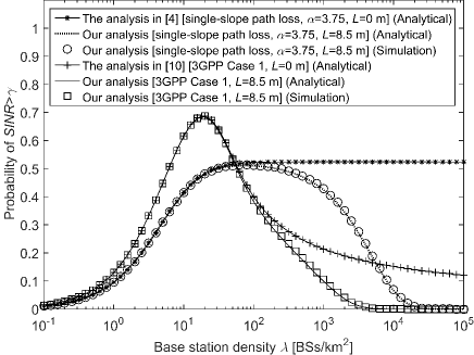
Fig. 2: $p^{{\rm{cov}}}\left(\lambda,\gamma\right)$ vs. $\lambda$ with $\gamma=0\,\textrm{dB}$ (Rayleigh fading only).

As can be observed from Fig. 2, our analytical results given by Theorem 1 and Lemma 2 match the simulation results very well, which validates the accuracy of our analysis. From Fig. 2, we can draw the following observations, which confirm our discussion in Section I:

• For the single-slope path loss model with $L=0$ m, the BS density does NOT matter, since the coverage probability approaches a constant for UDNs [4], e.g., $\lambda>10^{2}\,\textrm{BSs/km}^{2}$.

• For the 3GPP Case 1 path loss model with $L=0$ m, the BS density DOES matter, since that coverage probability will decrease as $\lambda$ increases when the network is dense enough, e.g., $\lambda>20\,\textrm{BSs/km}^{2}$, due to the transition of a large number of interference paths from NLoS to LoS [10].

• For both the 3GPP Case 1 and the single-slope path loss model shown in (6), when $L=8.5$ m, the coverage probability shows a determined trajectory toward zero in the UDN regime as explained in Theorem 3.

V-B Validation of Theorem 3 on the ASE Crash

In Fig. 3, we show the results of $A^{{\rm{ASE}}}\left(\lambda,\gamma_{0}\right)$ with $\gamma_{0}=0\,\textrm{dB}$.

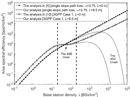
Fig. 3: $A^{{\rm{ASE}}}\left(\lambda,\gamma_{0}\right)$ vs. $\lambda$ with $\gamma_{0}=0\,\textrm{dB}$ (Rayleigh fading only).

Due to the significant accuracy of our analysis on $p^{{\rm{cov}}}\left(\lambda,\gamma\right)$ demonstrated in Fig. 2, we only show analytical results of $A^{{\rm{ASE}}}\left(\lambda,\gamma_{0}\right)$ in Fig. 3, because $A^{{\rm{ASE}}}\left(\lambda,\gamma_{0}\right)$ is computed from $p^{{\rm{cov}}}\left(\lambda,\gamma\right)$ as discussed in Subsection IV-B.

Fig. 3 is essentially the same as Fig. 1 with the same marker styles, except that the results for the simplistic single-slope path loss model with $L=8.5$ m are also plotted. From Fig. 3, we can confirm the key observations presented in Section I:

• For the single-slope path loss model with $L=0$ m, the ASE performance scales linearly with $\lambda$ [4]. The result is promising, but it might not be the truth in reality.

• For the 3GPP Case 1 path loss model with $L=0$ m, the ASE suffers from a slow growth or even a small decrease when $\lambda\in\left[20,200\right]\,\textrm{BSs/km}^{2}$, i.e., the ASE Crawl [10]. After the ASE Crawl, the ASE grows almost linearly again as the network further evolves to a UDN, e.g., $\lambda>10^{3}\thinspace\textrm{BSs/km}^{2}$ [10].

• For both path loss models with $L=8.5$ m, the ASE suffers from severe performance loss in UDNs due to the ASE Crash, as explained in Theorem 3.

• Here, we have established a baseline ASE Crash performance with the assumptions of “3GPP Case 1, $L=8.5$ m, Rayleigh fading only”. In the following subsections, all of the numerical results will be compared against such baseline ASE Crash performance to show the performance impacts of various factors.

V-C The Performance Impact of $L$ on the ASE Crash

In Fig. 4, we show the results of $A^{{\rm{ASE}}}\left(\lambda,\gamma_{0}\right)$ with $\gamma_{0}=0\,\textrm{dB}$ and various values of $L$. We assume that the UE antenna height is still 1.5 m, but the BS antenna height changes to 5 m, 10 m and 20 m, respectively.

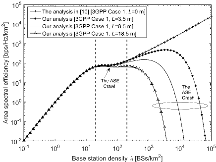
Fig. 4: $A^{{\rm{ASE}}}\left(\lambda,\gamma_{0}\right)$ vs. $\lambda$ with $\gamma_{0}=0\,\textrm{dB}$ and various $L$ (Rayleigh fading only).

Accordingly, $L$ takes the values of 3.5 m, 8.5 m and 18.5 m, respectively. Our key conclusions are summarized in the following:

• The larger the $L$, the severer the ASE Crash. This is because a larger $L$ implies a tighter cap on the signal power and the interference power, which leads to an earlier arrival of $\bar{\gamma}=1$ in (21) and thus the ASE Crash.

• Compared with the baseline ASE Crash performance, the reduction of $L$ from $8.5$ m to $3.5$ m can delay the ASE Crash from around $\lambda=10^{4}\thinspace\textrm{BSs/km}^{2}$ to around $\lambda=4\times 10^{4}\thinspace\textrm{BSs/km}^{2}$ when the ASE hits 1 $\textrm{bps/Hz/km}^{2}$. However, it is important to note that the ASE with $L=3.5$ m peaks at around $\lambda^{*}=3000\thinspace\textrm{BSs/km}^{2}$, but it still suffers from a 60 % loss compared with that with $L=0$ m at $\lambda^{*}$.

V-D The Performance Impact of Antenna Pattern and Downtilt on the ASE Crash

As discussed in Section III, via downtilt in the vertical domain, a practical antenna can target its antenna beam towards a given direction, which may affect the ASE Crash behavior. Here, we adopt the antenna pattern and downtilt model proposed in [21]. More specifically, in our analysis, the path loss function $\zeta\left(w\right)$ in (2) should be replaced by $\zeta\left(w\right)10^{\frac{1}{10}G\left(\varphi,\theta,\theta_{\textrm{tilt}}\right)}$, where $G\left(\varphi,\theta,\theta_{\textrm{tilt}}\right)$ is the antenna gain in the dB unit and it can be expressed by

$$G\left(\varphi,\theta,\theta_{\textrm{tilt}}\right)=G_{\textrm{M}}+G_{\textrm{H}}\left(\varphi\right)+G_{\textrm{V}}\left(\theta,\theta_{\textrm{tilt}}\right),$$ (35)

where $\varphi$ and $\theta$ are the angles of arrival in the horizontal and vertical planes, respectively, $\theta_{\textrm{tilt}}$ is the electrical downtilt angle of the vertical antenna beam, $G_{\textrm{M}}$ is the maximum antenna gain in dB, $G_{\textrm{H}}\left(\varphi\right)$ is the horizontal attenuation offset in dB, and $G_{\textrm{V}}\left(\theta,\theta_{\textrm{tilt}}\right)$ is the vertical attenuation offset in dB.

Considering a 4-element half-wave dipole antenna, we have $G_{\textrm{M}}=8.15\,\textrm{dB}$ [21]. For the horizontal pattern, as discussed in Section III, we consider a omni-directional antenna, i.e., $G_{\textrm{H}}\left(\varphi\right)=0\,\textrm{dB}$. For the vertical pattern, $G_{\textrm{V}}\left(\theta,\theta_{\textrm{tilt}}\right)$ is formulated according to [21] as

$$G_{\textrm{V}}\left(\theta,\theta_{\textrm{tilt}}\right)=\max\left\{10\log_{10}\left|\cos^{n}\left(\theta-\theta_{\textrm{tilt}}\right)\right|,F_{\textrm{V}}\right\},$$ (36)

where $n$ equals to 47.64 for a 4-element half-wave dipole antenna with a vertical half-power band-width (HPBW) of $B_{\textrm{V}}=19.5$ degrees, and $F_{\textrm{V}}$ is the vertical side-lobe level (SLL), which is set to -12 dB in [21]. As discussed in Section III, it is important to note that in practice $\theta_{\textrm{tilt}}$ becomes larger as the BS density $\lambda$ increases. According to [22], $\theta_{\textrm{tilt}}$ can be empirically modeled as

$$\theta_{\textrm{tilt}}=\arctan\left(\frac{L}{r^{\textrm{cov}}}\right)+zB_{\textrm{V}},$$ (37)

where $r^{\textrm{cov}}$ is the average distance from a cell-edge UE to its serving BS given by $r^{\textrm{cov}}=\sqrt{\frac{1}{\lambda\pi}}$ in our analysis, and $z$ is an empirical parameter achieving a good trade-off between the received signal power and the resulting inter-cell interference. In [22], $z$ is set to 0.7.

Plugging (37) into (36), we can obtain the antenna gain $G\left(\varphi,\theta,\theta_{\textrm{tilt}}\right)$ considering practical antenna pattern and downtilt. Such results are illustrated in Fig. 5.

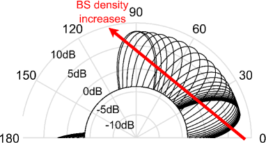
Fig. 5: $G\left(\varphi,\theta,\theta_{\textrm{tilt}}\right)$ vs. $\theta$ for a 4-element half-wave dipole antenna [21, 22].

From this figure, we can observe that the downtilt angle of the vertical antenna beam gradually increases from around 10 degrees to 90 degrees as the network densifies, and the maximum antenna gain is $G_{\textrm{M}}=8.15\,\textrm{dB}$ at the direction of such downtilt angle.

Based on the results of $G\left(\varphi,\theta,\theta_{\textrm{tilt}}\right)$ displayed in Fig. 5, we investigate the performance of $A^{{\rm{ASE}}}\left(\lambda,\gamma_{0}\right)$ with practical antenna pattern and downtilt in Fig. 6.

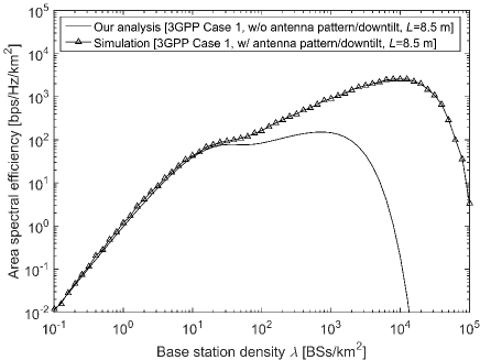
Fig. 6: $A^{{\rm{ASE}}}\left(\lambda,\gamma_{0}\right)$ vs. $\lambda$ with $\gamma_{0}=0\,\textrm{dB}$ and the practical antenna pattern and downtilt shown in Fig. 5 (Rayleigh fading only).

Our key conclusions from Fig. 6 are drawn as follows:

• The practical antenna pattern and downtilt shown in Fig. 5 help to alleviate the ASE Crash because they constrain the BS energy emission within certain geometrical areas. However, the ASE Crash still emerges in UDNs because the cap on the signal power persists, even if the BS antenna faces downward with a downtilt angle of 90 degrees.

• Compared with the baseline ASE Crash performance, the practical antenna pattern and downtilt can delay the ASE Crash from around $\lambda=10^{4}\thinspace\textrm{BSs/km}^{2}$ to more than $\lambda=10^{5}\thinspace\textrm{BSs/km}^{2}$ when the ASE declines to 1 $\textrm{bps/Hz/km}^{2}$.

V-E The Performance Impact of Rician Fading on the ASE Crash

In Fig. 7, we investigate the performance of $A^{{\rm{ASE}}}\left(\lambda,\gamma_{0}\right)$ under the assumptions of Rayleigh fading for NLoS transmissions and Rician fading ($K=10$) for LoS transmissions.

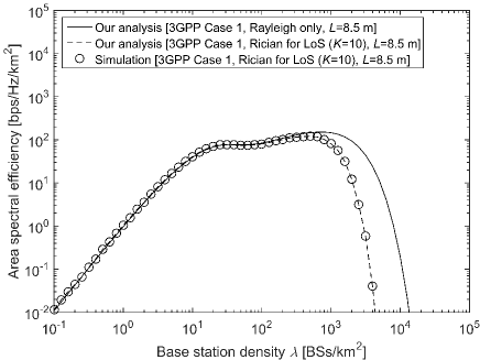
Fig. 7: $A^{{\rm{ASE}}}\left(\lambda,\gamma_{0}\right)$ vs. $\lambda$ with $\gamma_{0}=0\,\textrm{dB}$ (Rayleigh fading for NLoS transmissions and Rician fading ($K=10$) for LoS transmissions).

The analytical results are obtained from Theorem 1 and Lemma 4 presented in Subsection IV-D. Fig. 7 shows that our analytical results match the simulation results very well, which validates the accuracy of our analysis. Our key conclusions from Fig. 7 are summarized as follows:

• We can see that Rician fading makes the ASE Crash worse, which takes effect earlier than the case with Rayleigh fading. The intuition is that the randomness in channel fluctuation associated with Rician fading is much weaker than that associated with Rayleigh fading due to the large $K$ factor in UDNs [6]. With Rayleigh fading, some UE in outage might be opportunistically saved by favorable channel fluctuation of the signal power, while with Rician fading, such outage case becomes more deterministic due to lack of channel variation, thus leading to a severer ASE Crash.

• Compared with the baseline ASE Crash performance, the investigated Rician fading will bring forward the ASE Crash from around $\lambda=10^{4}\thinspace\textrm{BSs/km}^{2}$ to $\lambda=3\times 10^{3}\thinspace\textrm{BSs/km}^{2}$ when the ASE is merely 1 $\textrm{bps/Hz/km}^{2}$.

V-F The Performance Impact of 3GPP Case 2 on the ASE Crash

In this subsection, we investigate the ASE performance for 3GPP Case 2, which has been discussed in Subsection IV-E. The parameters in the LoS probability function $\textrm{Pr}^{\textrm{L}}\left(w\right)$ of 3GPP Case 2 are set to $R_{1}=156$ m and $R_{2}=30$ m [5]. First, we directly apply the numerical integration in Theorem 1 to evaluate the ASE result for 3GPP Case 2. Second, in order to show the versatility of the studied 3GPP Case 1 with the linear LoS probability function shown in (33), as in [10], we adopt the technique of approximating the LoS probability function of 3GPP Case 2 shown in (34) by a 3-piece linear function as

$$\textrm{Pr}^{\textrm{L}}\left(w\right)=\begin{cases}\begin{array}[]{l}1,\\ 1-\frac{w-d_{1}}{d_{2}-d_{1}},\\ 0,\end{array}&\begin{array}[]{l}L<w\leq d_{1}\\ d_{1}<w\leq d_{2}\\ w>d_{2}\end{array}\end{cases},$$ (38)

where $d_{1}$ and $d_{2}$ are set to 18.4 m and 117.1 m, respectively. Note that $d_{1}$ is chosen as 18.4 m because $\textrm{Pr}^{\textrm{L}}\left(d_{1}\right)=0.999\approx 1$ in (34). Besides, the value of $d_{2}$ is obtained from the requirement that $\textrm{Pr}^{\textrm{L}}\left(r\right)$ in (38) should go through the point $\left(\frac{R_{1}}{\ln 10},0.5\right)$, which is the crucial point connecting the two segments in $\textrm{Pr}^{\textrm{L}}\left(r\right)$ of 3GPP Case 2 given by (34). Note that the approximation of (38) can be easily improved by fitting the LoS probability function with more than three pieces in (38). For clarity, the combined case with the path loss function of (32) and the 3-piece LoS probability function of (38) is referred to as the Approximated 3GPP Case 2. Based on Theorem 1, we can readily extend the results in Appendix E to analyze the Approximated 3GPP Case 2 in a tractable manner. The details are very similar to those in [10] and thus omitted here for brevity.

In Fig. 8, we show the results of $A^{\textrm{ASE}}\left(\lambda,\gamma_{0}\right)$ for 3GPP Case 2.

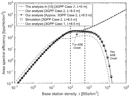
Fig. 8: $A^{{\rm{ASE}}}\left(\lambda,\gamma_{0}\right)$ vs. $\lambda$ with $\gamma_{0}=0\,\textrm{dB}$ for 3GPP Case 2 (Rayleigh fading only).

As can be seen from Fig. 8, the results of the Approximated 3GPP Case 2 based on (38) match those of 3GPP Case 2 well, thus showing the extensibility of our analysis with the linear LoS probability function. More importantly, all the observations in Subsection V-B are qualitatively valid for Fig. 8 except for some quantitative deviation. In more detail,

• The BS density range of the ASE Crawl for 3GPP Case 2 is around $\lambda\in\left[200,600\right]\,\textrm{BSs/km}^{2}$. And the ASE also suffers from severe performance loss in UDNs, e.g., $\lambda>10^{3}\,\textrm{BSs/km}^{2}$.

• Compared with the baseline ASE Crash performance, the alternative path loss model 3GPP Case 2 can delay the ASE Crash from around $\lambda=10^{4}\thinspace\textrm{BSs/km}^{2}$ to a bit more than $\lambda=10^{4}\thinspace\textrm{BSs/km}^{2}$ when the ASE crashes to 1 $\textrm{bps/Hz/km}^{2}$.

V-G Key Takeaways

The key takeaways of our study are summarized as follows,

• As explained in Subsection IV-C, the fundamental reason of the ASE crash is rooted in the geometry of BS deployments. Consequently, as shown in previous subsections, both the path loss models and the multi-path fading models do not change the conclusion of the ASE crash. It should be noted that even if $L=0$, we may still end up with $\bar{\gamma}\rightarrow 1$ in (21), which leads to the ASE Crash. One example is that if the BSs are deployed on a circle or on the surface of a cylinder, then we would have two base stations that are equally distant from the UE located at the center. Another example is that in a very densely populated pedestrian street where BSs cannot be placed anywhere on the street itself, but only on walls abutting the street, we would also observe two base stations having an equal distance from the UE standing in the middle of the street [26]. Compared with the above two interesting examples, our paper analyzes a more likely to happen scenario with random BS deployment, and establishes the significant problem that these networks will face if the antenna height issue is not considered in practice.

• Regarding the solutions to avoid the ASE crash, a straightforward one is to lower the BS antenna height in 5G UDNs, so that the ASE behavior of such networks would roll back to our previous results in [9, 10]. Such proposed new BS deployment will allow to realize the potential gains of UDNs, but needs a revolution on BS architectures and network deployment in the future. Some new research challenges are as follows:

  • New measurement campaigns for the UE-height channels.

  • Futuristic BS architectures/hardware that are anti-vandalism/anti-theft/anti-hacking at low-height positions.

  • New research avenues due to the emergence of fast time-variant shadow fading due to random movement of UE-height objects, e.g., cars. Interesting topics include new UE association strategies, agile power control, fast link adaptation, etc.

  • Terrain-dependent network performance analysis considering hills, elevated roads, etc.

  • New inter-BS communication means based on ground waves.

• Another solution to mitigate the ASE crash is interference coordination. In order to mitigate inter-cell interference, LTE Release 8 incorporates the inter-cell interference coordination (ICIC) features [27], which provide mechanisms to coordinate RB usage among neighboring BSs, e.g. high interference indicator (HII) and overload indicator (OI) for the uplink and relative narrow-band transmit power (RNTP) for the downlink. These features may be used in current macrocell base stations, but not widely, due to overhead and delay issues in the backhaul interface as well as the complexity of finding a good solution using local measures. In practice, such features have not been used in small cells, the topic of the paper. Moreover, it is worth noting that LTE Release 13 incorporates a new small cell feature to enable dynamic muting of small cell BSs [27] by the use of discovery reference signals. Using such mechanism to mitigate the overwhelming interference causing the ASE Crash is a topic for further study.

• Another solution to mitigate the ASE crash is beam steering/shaping using multi-antenna technologies. However, it should be noted that sub-6GHz small cell products are of small form factor and targeted at a low price. Thus, the number of antennas that can be placed in the small cell BS is quite limited, which in turn limits such beam steering/shaping capabilities. Such techniques are more beneficial for millimeter wave solutions with a larger number of antennas, but they are out of the scope of this paper, because this technology requires a completely different modeling, as the 3GPP has done in the standardization of the 5G networks [28]. In more detail, we need to consider new millimeter wave communication features, such as short-range coverage, the blockage effect, very low inter-cell interference, molecule absorption and re-radiation, high Doppler shift, etc. Moreover, note that bringing beam steering and beam shaping into the paper would mandate the study on the channel correlation among different UEs. As a results, millimeter wave transmissions with multiple antennas to mitigate the ASE Crash are for further study.

VI Conclusion

We presented a new and significant theoretical discovery, i.e., the serious problem of the ASE Crash. If the absolute height difference between BS antenna and UE antenna is larger than zero, then the ASE performance will continuously decrease toward zero with the network densification for UDNs. One way to overcome the ASE Crash is to lower the BS antenna height to the UE antenna height, which will revolutionize the approach of BS architecture and network deployment in the future. Other ways to counter-measure the ASE Crash could be pro-active muting of BSs, dynamic beam tracking, cooperation of neighbouring BSs, and so on, which are worth further studying in the context of UDNs.

Appendix A: Proof of Theorem 1

In (10), $T_{n}^{{\rm{L}}}$ and $T_{n}^{{\rm{NL}}}$ are the components of the coverage probability for the case when the signal comes from the $n$-th piece LoS path and for the case when the signal comes from the $n$-th piece NLoS path, respectively. The calculation of $T_{n}^{{\rm{L}}}$ is based on (11) and Lemma 2. In (11), $f_{R,n}^{{\rm{L}}}\left(r\right)$ characterizes the geometrical density function of the typical UE with no other LoS BS and no NLoS BS providing a better link to the typical UE than its serving BS (a BS with the $n$-th piece LoS path). The calculation of $T_{n}^{{\rm{NL}}}$ is based on (12) and Lemma 2. The interpretation of (12) is similar to that for the calculation of $T_{n}^{{\rm{L}}}$.

Appendix B: Proof of Lemma 2

In Lemma 2, ${\rm{Pr}}\left[\frac{P\zeta_{n}^{{\rm{L}}}\left(\sqrt{r^{2}+L^{2}}\right)h}{I_{{\rm{agg}}}+P_{{\rm{N}}}}>\gamma\right]$ can be calculated as

${\rm{Pr}}\left[\frac{P\zeta_{n}^{{\rm{L}}}\left(\sqrt{r^{2}+L^{2}}\right)h}{I_{{\rm{agg}}}+P_{{\rm{N}}}}>\gamma\right]$

$$= \mathbb{E}_{\left[I_{{\rm{agg}}}\right]}\left\{\textrm{Pr}\left[h>\frac{\gamma\left(I_{{\rm{agg}}}+P_{{\rm{N}}}\right)}{P\zeta_{n}^{{\rm{L}}}\left(\sqrt{r^{2}+L^{2}}\right)}\right]\right\}$$ (39)

$$= \mathbb{E}_{\left[I_{{\rm{agg}}}\right]}\left\{\bar{F}_{H}\left(\frac{\gamma\left(I_{{\rm{agg}}}+P_{{\rm{N}}}\right)}{P\zeta_{n}^{{\rm{L}}}\left(\sqrt{r^{2}+L^{2}}\right)}\right)\right\},$$

where $\mathbb{E}_{\left[X\right]}\left\{\cdot\right\}$ denotes the expectation operation taking the expectation over the variable $X$ and $\bar{F}_{H}\left(h\right)$ denotes the CCDF of RV $h$. Since we assume $h$ to be an exponential RV, we have $\bar{F}_{H}\left(h\right)=\exp\left(-h\right)$ and thus (39) can be further derived as

${\rm{Pr}}\left[\frac{P\zeta_{n}^{{\rm{L}}}\left(\sqrt{r^{2}+L^{2}}\right)h}{I_{{\rm{agg}}}+P_{{\rm{N}}}}>\gamma\right]$

$$= \mathbb{E}_{\left[I_{{\rm{agg}}}\right]}\left\{\bar{F}_{H}\left(\frac{\gamma\left(I_{{\rm{agg}}}+P_{{\rm{N}}}\right)}{P\zeta_{n}^{{\rm{L}}}\left(\sqrt{r^{2}+L^{2}}\right)}\right)\right\}$$ (40)

$$= \exp\left(-\frac{\gamma P_{{\rm{N}}}}{P\zeta_{n}^{{\rm{L}}}\left(\sqrt{r^{2}+L^{2}}\right)}\right)$$

$$\times\mathbb{E}_{\left[I_{{\rm{agg}}}\right]}\left\{\exp\left(-\frac{\gamma I_{{\rm{agg}}}}{P\zeta_{n}^{{\rm{L}}}\left(\sqrt{r^{2}+L^{2}}\right)}\right)\right\}$$

$$= \exp\left(-\frac{\gamma P_{{\rm{N}}}}{P\zeta_{n}^{{\rm{L}}}\left(\sqrt{r^{2}+L^{2}}\right)}\right)$$

$$= \times\mathscr{L}_{I_{{\rm{agg}}}}^{{\rm{L}}}\left(\frac{\gamma}{P\zeta_{n}^{{\rm{L}}}\left(\sqrt{r^{2}+L^{2}}\right)}\right),$$

where $\mathscr{L}_{I_{{\rm{agg}}}}^{{\rm{L}}}\left(s\right)$ is the Laplace transform of RV $I_{{\rm{agg}}}$ evaluated at $s$ on the condition of the event that the typical UE is associated with a BS with a LoS path. Note that $\exp\left(-\frac{\gamma P_{{\rm{N}}}}{P\zeta_{n}^{{\rm{L}}}\left(\sqrt{r^{2}+L^{2}}\right)}\right)$ measures the probability that the signal power exceeds the noise power by a factor of at least $\gamma$, and $\mathscr{L}_{I_{{\rm{agg}}}}^{{\rm{L}}}\left(\frac{\gamma}{P\zeta_{n}^{{\rm{L}}}\left(\sqrt{r^{2}+L^{2}}\right)}\right)$ measures the probability that the signal power exceeds the aggregate interference power by a factor of at least $\gamma$. Since $h$ follows an exponential distribution, the product of the above probabilities yields the probability that the signal power exceeds the sum power of the noise and the aggregate interference by a factor of at least $\gamma$. Based on the presented UAS, we can derive $\mathscr{L}_{I_{{\rm{agg}}}}^{{\rm{L}}}\left(s\right)$ as

$\mathscr{L}_{I_{{\rm{agg}}}}^{{\rm{L}}}\left(s\right)$

$$= \mathbb{E}_{\left[I_{{\rm{agg}}}\right]}\left\{\left.\exp\left(-sI_{{\rm{agg}}}\right)\right|B^{{\rm{L}}}\right\}$$ (41)

$$= \mathbb{E}_{\left[\Phi,\left\{\beta_{i}\right\},\left\{g_{i}\right\}\right]}\left\{\left.\exp\left(-s\sum_{i\in\Phi/b_{o}}P\beta_{i}\left(w\right)g_{i}\right)\right|B^{{\rm{L}}}\right\}.$$

According to [4], $\mathbb{E}_{\left[g\right]}\left\{\left.\exp\left(-sP\beta\left(w\right)g\right)\right|B^{{\rm{L}}}\right\}$ in (41) should consider interference from both LoS and NLoS paths. Thus, $\mathscr{L}_{I_{{\rm{agg}}}}^{{\rm{L}}}\left(s\right)$ can be further derived as

$\mathscr{L}_{I_{{\rm{agg}}}}^{{\rm{L}}}\left(s\right)$

$$= \exp\left(-2\pi\lambda\int_{r}^{+\infty}\textrm{{\rm{Pr}}}^{{\rm{L}}}\left(\sqrt{u^{2}+L^{2}}\right)\right.$$

$$\times\left[1-\mathbb{E}_{\left[g\right]}\left\{\exp\left(-sP\zeta^{{\rm{L}}}\left(\sqrt{u^{2}+L^{2}}\right)g\right)\right\}\right]udu$$

$$-2\pi\lambda\int_{r_{1}}^{+\infty}\left[1-\textrm{{\rm{Pr}}}^{{\rm{L}}}\left(\sqrt{u^{2}+L^{2}}\right)\right]$$

$$\left.\times\left[1-\mathbb{E}_{\left[g\right]}\left\{\exp\left(-sP\zeta^{{\rm{NL}}}\left(\sqrt{u^{2}+L^{2}}\right)g\right)\right\}\right]udu\right)$$

$$= \exp\left(-2\pi\lambda\int_{r}^{+\infty}\frac{\textrm{{\rm{Pr}}}^{{\rm{L}}}\left(\sqrt{u^{2}+L^{2}}\right)u}{1+\left(sP\zeta^{{\rm{L}}}\left(\sqrt{u^{2}+L^{2}}\right)\right)^{-1}}du\right)$$

$$\times\exp\left(-2\pi\lambda\int_{r_{1}}^{+\infty}\frac{\left[1-\textrm{{\rm{Pr}}}^{{\rm{L}}}\left(\sqrt{u^{2}+L^{2}}\right)\right]u}{1+\left(sP\zeta^{{\rm{NL}}}\left(\sqrt{u^{2}+L^{2}}\right)\right)^{-1}}du\right).$$

Plugging $s=\frac{\gamma}{P\zeta_{n}^{{\rm{L}}}\left(\sqrt{r^{2}+L^{2}}\right)}$ into (LABEL:eq:laplace_term_LoS_UAS1_general_seg_part2) and further plugging (LABEL:eq:laplace_term_LoS_UAS1_general_seg_part2) into (40), we can obtain the general expression of ${\rm{Pr}}\left[\frac{P\zeta_{n}^{{\rm{L}}}\left(\sqrt{r^{2}+L^{2}}\right)h}{I_{{\rm{agg}}}+P_{{\rm{N}}}}>\gamma\right]$ shown in (15).

In a similar way, we can obtain the general expression of ${\rm{Pr}}\left[\frac{P\zeta_{n}^{{\rm{NL}}}\left(\sqrt{r^{2}+L^{2}}\right)h}{I_{{\rm{agg}}}+P_{{\rm{N}}}}>\gamma\right]$ shown in (17), which concludes our proof.

Appendix C: Proof of Theorem 3

By applying the theory of limits on $p^{{\rm{cov}}}\left(\lambda,\gamma\right)$ derived in Theorem 1, we can obtain that $\underset{\lambda\rightarrow+\infty}{\lim}p^{{\rm{cov}}}\left(\lambda,\gamma\right)=\underset{\lambda\rightarrow+\infty}{\lim}T_{1}^{{\rm{L}}}+\underset{\lambda\rightarrow+\infty}{\lim}T_{1}^{{\rm{NL}}}$. This is because

• When $\lambda\rightarrow+\infty$, the typical 2D distance $r$ from the UE to its serving BS $b_{o}$ approaches zero, i.e., $r\rightarrow 0$, which should be dominantly characterized by either the first-piece LoS path loss function or the first-piece NLoS path loss function due to the short-distance link and $L$ is smaller than $d_{1}$ in practical SCNs [6, 5]; and

• According to Appendix A, $T_{1}^{{\rm{L}}}$ and $T_{1}^{{\rm{NL}}}$ measure nothing but the components of the coverage probability for the cases that the signal comes from the first-piece LoS path and that the signal comes from the first-piece NLoS path, respectively.

Moreover, when $\lambda\rightarrow+\infty$, we have $\underset{\lambda\rightarrow+\infty}{\lim}T_{1}^{{\rm{NL}}}=0$ due to $\underset{\lambda\rightarrow+\infty}{\lim}f_{R,1}^{{\rm{NL}}}\left(r\right)=0$. In more detail, $f_{R,1}^{{\rm{NL}}}\left(r\right)$ approaches zero when $\lambda\rightarrow+\infty$, i.e., $r\rightarrow 0$, because

• According to (14), $\underset{r\rightarrow 0}{\lim}r_{2}=\underset{r_{2}}{\arg}\left\{\zeta^{{\rm{L}}}\left(\sqrt{r_{2}^{2}+L^{2}}\right)=\zeta_{1}^{{\rm{NL}}}\left(L\right)\right\}\stackrel{{\scriptstyle\bigtriangleup}}{{=}}r_{2}^{\textrm{min}}$, which is a non-zero value due to the non-zero value of $L$.

• Thus, the term $\exp\left(-\int_{0}^{r_{2}}{\rm{Pr}}^{{\rm{L}}}\left(\sqrt{u^{2}+L^{2}}\right)2\pi u\lambda du\right)$ in (12) can be upper-bounded by $\exp\left(-{\rm{Pr}}^{{\rm{L}}}\left(\sqrt{\left(r_{2}^{\textrm{min}}\right)^{2}+L^{2}}\right)\pi\lambda\left(r_{2}^{\textrm{min}}\right)^{2}\right)$, which approaches zero when $\lambda\rightarrow+\infty$. Note that we assume ${\rm{Pr}}^{{\rm{L}}}\left(w\right)$ to be a monotonically decreasing function with respect to $w$ as explained in Section III.

• Hence, we can obtain $\underset{\lambda\rightarrow+\infty}{\lim}f_{R,1}^{{\rm{NL}}}\left(r\right)=0$ considering the definition of $f_{R,1}^{{\rm{NL}}}\left(r\right)$ in (12).

Therefore, we can claim that $\underset{\lambda\rightarrow+\infty}{\lim}p^{{\rm{cov}}}\left(\lambda,\gamma\right)=\underset{\lambda\rightarrow+\infty}{\lim}T_{1}^{{\rm{L}}}$, which is in line with the intuitive fact that when $\lambda\rightarrow+\infty$, the coverage probability should be mainly contributed by the case that the signal comes from the first-piece LoS path.

Next, we show that $\underset{\lambda\rightarrow+\infty}{\lim}{\rm{Pr}}\left[\frac{P\zeta_{1}^{{\rm{L}}}\left(\sqrt{r^{2}+L^{2}}\right)h}{I_{{\rm{agg}}}+N_{0}}>\gamma\right]=0$, so that we can get $\underset{\lambda\rightarrow+\infty}{\lim}T_{1}^{{\rm{L}}}=0$. From (15) and (16), we have

${\rm{Pr}}\left[\frac{P\zeta_{1}^{{\rm{L}}}\left(\sqrt{r^{2}+L^{2}}\right)h}{I_{{\rm{agg}}}+N_{0}}>\gamma\right]$

$$< \exp\left(-2\pi\lambda\int_{r}^{+\infty}\frac{{\rm{Pr}}^{{\rm{L}}}\left(\sqrt{u^{2}+L^{2}}\right)u}{1+\left(\frac{\gamma P\zeta^{{\rm{L}}}\left(\sqrt{u^{2}+L^{2}}\right)}{P\zeta_{1}^{{\rm{L}}}\left(\sqrt{r^{2}+L^{2}}\right)}\right)^{-1}}du\right)$$ (43)

$$< \exp\left(-2\pi\lambda\int_{r}^{\tau r}\frac{{\rm{Pr}}^{{\rm{L}}}\left(\sqrt{u^{2}+L^{2}}\right)u}{1+\frac{1}{\gamma}\left(\frac{\sqrt{r^{2}+L^{2}}}{\sqrt{u^{2}+L^{2}}}\right)^{-\alpha_{1}^{{\rm{L}}}}}du\right)$$ (44)

$$< \exp\left(-2\pi\lambda\frac{{\rm{Pr}}^{{\rm{L}}}\left(\sqrt{\tau^{2}r^{2}+L^{2}}\right)\int_{r}^{\tau r}udu}{1+\frac{1}{\gamma}\left(\frac{\sqrt{r^{2}+L^{2}}}{\sqrt{\tau^{2}r^{2}+L^{2}}}\right)^{-\alpha_{1}^{{\rm{L}}}}}\right)$$ (45)

$$\overset{r\rightarrow 0}{<} \exp\left(-\frac{{\rm{Pr}}^{{\rm{L}}}\left(L\right)\left(\tau^{2}-1\right)}{1+\frac{1}{\gamma}}\right)\overset{\Delta}{=}\kappa,$$ (46)

where $\kappa$ is derived because

• As explained in Appendix A, (43) only considers the probability that the signal power beats the aggregate interference power from all LoS BSs by a factor of at least $\gamma$, which over-estimates the coverage probability. Besides, $s=\frac{\gamma}{P\zeta_{1}^{{\rm{L}}}\left(\sqrt{r^{2}+L^{2}}\right)}$ is plugged into (43).

• In (44), we further concentrate on the LoS interference that is relatively close to the UE, i.e., $u\in\left(r,\tau r\right],\left(1<\tau<+\infty\right)$. Besides, the first-piece LoS path loss function has also been used for such LoS interference, because when $r\rightarrow 0$ we have $\tau r\rightarrow 0$, which falls into the region that is dominantly characterized by the first-piece LoS path loss function.

• We arrive at (45) because (i) $\left(\frac{\sqrt{r^{2}+L^{2}}}{\sqrt{u^{2}+L^{2}}}\right)^{-\alpha_{1}^{{\rm{L}}}}<\left(\frac{\sqrt{r^{2}+L^{2}}}{\sqrt{\tau^{2}r^{2}+L^{2}}}\right)^{-\alpha_{1}^{{\rm{L}}}},u\in\left(r,\tau r\right]$; and (ii) ${\rm{Pr}}^{{\rm{L}}}\left(\sqrt{u^{2}+L^{2}}\right)>{\rm{Pr}}^{{\rm{L}}}\left(\sqrt{\tau^{2}r^{2}+L^{2}}\right),u\in\left(r,\tau r\right]$, since ${\rm{Pr}}^{{\rm{L}}}\left(w\right)$ is a monotonically decreasing function with respect to $w$ as explained in Section III.

• Finally, we plug $\underset{\lambda\rightarrow+\infty}{\lim}{\rm{Pr}}^{{\rm{L}}}\left(\sqrt{\tau^{2}r^{2}+L^{2}}\right)={\rm{Pr}}^{{\rm{L}}}\left(L\right)$, $\underset{\lambda\rightarrow+\infty}{\lim}\frac{\sqrt{r^{2}+L^{2}}}{\sqrt{\tau^{2}r^{2}+L^{2}}}=1$, $\int_{r}^{\tau r}udu=\frac{1}{2}\left(\tau^{2}-1\right)r^{2}$ and $\underset{\lambda\rightarrow+\infty}{\lim}\pi r^{2}\lambda=1$ into (45) to obtain (46). Note that we have $\underset{\lambda\rightarrow+\infty}{\lim}\pi r^{2}\lambda=1$ because the typical coverage radius, denoted by $\hat{r}$, permits $\underset{\lambda\rightarrow+\infty}{\lim}\pi\hat{r}^{2}\lambda=1$, i.e., the typical coverage area $\pi\hat{r}^{2}$ is in the order of $\frac{1}{\lambda}$. Hence, $\underset{\lambda\rightarrow+\infty}{\lim}\pi r^{2}\lambda=1$ holds because $r\rightarrow\hat{r}$ when $\lambda\rightarrow+\infty$.

Since $\tau$ takes an arbitrary and finite value, we have $\underset{\lambda\rightarrow+\infty}{\lim}{\rm{Pr}}\left[\frac{P\zeta_{1}^{{\rm{L}}}\left(\sqrt{r^{2}+L^{2}}\right)h}{I_{{\rm{agg}}}+N_{0}}>\gamma\right]=0$ because $\kappa$ can be reduced to any arbitrarily small value when $\tau$ is sufficiently large. For example, when ${\rm{Pr}}^{{\rm{L}}}\left(L\right)=0.8$, $\gamma=1$, and $\tau$ equals to a moderate value of 8, then $\kappa$ is smaller than $1\times 10^{-11}$. Therefore, according to the definition of $T_{1}^{{\rm{L}}}$ in (10), we can get $\underset{\lambda\rightarrow+\infty}{\lim}T_{1}^{{\rm{L}}}=\underset{\lambda\rightarrow+\infty}{\lim}p^{{\rm{cov}}}\left(\lambda,\gamma\right)=0$.

Furthermore, since $\gamma$ is arbitrary for $p^{{\rm{cov}}}\left(\lambda,\gamma\right)$, we can set $\gamma>\gamma_{0}$ and put the UE into a complete outage in UDNs, i.e., $\underset{\lambda\rightarrow+\infty}{\lim}\textrm{Pr}\left[\mathrm{SINR}>\gamma_{0}\right]\equiv 0$. Since the UDNs are now operating below the minimum working SINR $\gamma_{0}$, according to the definition of ASE in (19), we have $\underset{\lambda\rightarrow+\infty}{\lim}A^{\textrm{ASE}}\left(\lambda,\gamma_{0}\right)=0$, which completes our proof.

Appendix D: Proof of Lemma 4

Let $SINR^{\textrm{L}}=\frac{P\zeta_{n}^{{\rm{L}}}\left(\sqrt{r^{2}+L^{2}}\right)h}{I_{{\rm{agg}}}+P_{{\rm{N}}}}$, then ${\rm{Pr}}\left[\frac{P\zeta_{n}^{{\rm{L}}}\left(\sqrt{r^{2}+L^{2}}\right)h}{I_{{\rm{agg}}}+P_{{\rm{N}}}}>\gamma\right]$ can be reformulated as

${\rm{Pr}}\left[SINR^{\textrm{L}}>\gamma\right]$

$$= {\rm{Pr}}\left[\frac{1}{SINR^{\textrm{L}}}<\frac{1}{\gamma}\right]$$ (47)

$$= \int_{0}^{\frac{1}{\gamma}}f_{\frac{1}{SINR^{\textrm{L}}}}\left(x\right)dx$$

$$\overset{(a)}{=} \int_{0}^{\frac{1}{\gamma}}\frac{1}{2\pi}\mathcal{\int_{\mathrm{-}\infty}^{\infty}}\mathcal{F}_{\frac{1}{SINR^{\textrm{L}}}}(\omega)\exp\left(-\textrm{j}\omega x\right)d\omega dx$$

$$\overset{(b)}{=} \int_{-\infty}^{+\infty}\left(\frac{1-\exp\left(\frac{\textrm{j}\omega}{\gamma}\right)}{2\pi\textrm{j}\omega}\right)\mathcal{F}_{\frac{1}{SINR^{\textrm{L}}}}(\omega)d\omega,$$

where in ($a$) $\mathcal{F}_{\frac{1}{SINR^{\textrm{L}}}}(\omega)$ denotes the characteristic function of $\frac{1}{SINR^{\textrm{L}}}$ and in ($b$) the integral with respect to $x$ has been computed to simplify the expression. Furthermore, $\mathcal{F}_{\frac{1}{SINR^{\textrm{L}}}}(\omega)$ can be written as

$\mathcal{F}_{\frac{1}{SINR^{\textrm{L}}}}(\omega)$

$$\overset{(a)}{=} \mathbb{E}_{\left[\frac{1}{SINR^{\textrm{L}}}\right]}\left\{\exp\left(\textrm{j}\omega\frac{1}{SINR^{\textrm{L}}}\right)\right\}$$ (48)

$$\overset{(b)}{=} \mathbb{E}_{\left[S^{{\rm{L}}},I_{{\rm{agg}}}^{{\rm{L}}},I_{{\rm{agg}}}^{{\rm{NL}}}\right]}\left\{\exp\left(\textrm{j}\omega\frac{I_{{\rm{agg}}}^{{\rm{L}}}+I_{{\rm{agg}}}^{{\rm{NL}}}+P_{{\rm{N}}}}{S^{{\rm{L}}}}\right)\right\}$$

$$= \mathbb{E}_{\left[S^{{\rm{L}}}\right]}\left\{\mathbb{E}_{\left[I_{{\rm{agg}}}^{{\rm{L}}}\right]}\left\{\exp\left(\textrm{j}\omega\frac{I_{{\rm{agg}}}^{{\rm{L}}}}{S^{{\rm{L}}}}\right)\right\}\right.$$

$$= \left.\times\mathbb{E}_{\left[I_{{\rm{agg}}}^{{\rm{NL}}}\right]}\left\{\exp\left(\textrm{j}\omega\frac{I_{{\rm{agg}}}^{{\rm{NL}}}}{S^{{\rm{L}}}}\right)\right\}\exp\left(\textrm{j}\omega\frac{P_{{\rm{N}}}}{S^{{\rm{L}}}}\right)\right\}$$

$$\overset{(c)}{=} \mathbb{E}_{\left[h\right]}\left\{\exp\left(\textrm{j}\omega\frac{P_{{\rm{N}}}}{P\zeta_{n}^{{\rm{L}}}\left(\sqrt{r^{2}+L^{2}}\right)h}\right)\right.$$

$$\times\mathbb{E}_{\left[\Phi^{{\rm{L}}},\left\{\beta_{i}^{{\rm{L}}}\right\},\left\{g_{i}^{{\rm{L}}}\right\}\right]}\left\{\exp\left(\textrm{j}\omega\frac{\sum_{i\in\Phi^{{\rm{L}}}}P\beta_{i}^{{\rm{L}}}g_{i}^{{\rm{L}}}}{P\zeta_{n}^{{\rm{L}}}\left(\sqrt{r^{2}+L^{2}}\right)h}\right)\right\}$$

$$\left.\times\mathbb{E}_{\left[\Phi^{{\rm{NL}}},\left\{\beta_{i}^{{\rm{NL}}}\right\},\left\{g_{i}^{{\rm{NL}}}\right\}\right]}\left\{\exp\left(\textrm{j}\omega\frac{\sum_{i\in\Phi^{{\rm{NL}}}}P\beta_{i}^{{\rm{NL}}}g_{i}^{{\rm{NL}}}}{P\zeta_{n}^{{\rm{L}}}\left(\sqrt{r^{2}+L^{2}}\right)h}\right)\right\}\right\},$$

where

• ($a$) comes from the definition of $\mathcal{F}_{\frac{1}{SINR^{\textrm{L}}}}(\omega)$ [25],

• ($b$) breaks down the expression of $SINR^{\textrm{L}}$, where $S^{\textrm{L}}=P\zeta_{n}^{{\rm{L}}}\left(\sqrt{r^{2}+L^{2}}\right)h$ and $h$ follows a non-central chi-squared distribution due to our assumption of Rician fading for LoS transmissions [25], $I_{{\rm{agg}}}^{{\rm{L}}}$ denotes the aggregated interference from LoS interfering BSs to the typical UE, and $I_{{\rm{agg}}}^{{\rm{NL}}}$ denotes the aggregated interference from NLoS interfering BSs to the typical UE,

• ($c$) further breaks down the expression of $I_{{\rm{agg}}}^{{\rm{L}}}$ and $I_{{\rm{agg}}}^{{\rm{NL}}}$. To take $I_{{\rm{agg}}}^{{\rm{L}}}$ as an example, we have $I_{{\rm{agg}}}^{{\rm{L}}}=\sum_{i\in\Phi^{{\rm{L}}}}P\beta_{i}^{{\rm{L}}}g_{i}^{{\rm{L}}}$, where $\Phi^{{\rm{L}}}$, $\beta_{i}^{{\rm{L}}}$ and $g_{i}^{{\rm{L}}}$ denote the set of LoS interfering BSs, the path loss of the $i$-th LoS interfering BS and the Rician fading power of the $i$-th LoS interfering BS.

We define $ISR_{{\rm{aggL}}}^{{\rm{L}}}=\mathbb{E}_{\left[\Phi^{{\rm{L}}},\left\{\beta_{i}^{{\rm{L}}}\right\},\left\{g_{i}^{{\rm{L}}}\right\}\right]}\left\{\exp\left(\textrm{j}\omega\frac{\sum_{i\in\Phi^{{\rm{L}}}}P\beta_{i}^{{\rm{L}}}g_{i}^{{\rm{L}}}}{P\zeta_{n}^{{\rm{L}}}\left(\sqrt{r^{2}+L^{2}}\right)h}\right)\right\}$, which is the LoS interference to LoS signal ratio and can be derived as

$ISR_{{\rm{aggL}}}^{{\rm{L}}}$

$$\overset{(a)}{=} \exp\left(-2\pi\lambda\int_{r}^{+\infty}\textrm{{\rm{Pr}}}^{{\rm{L}}}\left(\sqrt{u^{2}+L^{2}}\right)\right.$$ (49)

$$\left.\times\left(1-\mathbb{E}_{\left[g^{{\rm{L}}}\right]}\left\{\exp\left(\textrm{j}\omega\frac{\zeta^{{\rm{L}}}\left(\sqrt{u^{2}+L^{2}}\right)g^{{\rm{L}}}}{\zeta_{n}^{{\rm{L}}}\left(\sqrt{r^{2}+L^{2}}\right)h}\right)\right\}\right)udu\right),$$

where ($a$) is derived according to Campbell’s theorem [29] and the fact that any LoS interfering BS should stay away from the typical UE by at least $r$ (see Theorem 1). Since we assume that Rician fading is associated with LoS transmissions, $\mathbb{E}_{\left[g^{{\rm{L}}}\right]}\left\{\exp\left(\textrm{j}\omega\frac{\zeta^{{\rm{L}}}\left(\sqrt{u^{2}+L^{2}}\right)g^{{\rm{L}}}}{\zeta_{n}^{{\rm{L}}}\left(\sqrt{r^{2}+L^{2}}\right)h}\right)\right\}$ in (49) can be further written as

$\mathbb{E}_{\left[g^{{\rm{L}}}\right]}\left\{\exp\left(\textrm{j}\omega\frac{\zeta^{{\rm{L}}}\left(\sqrt{u^{2}+L^{2}}\right)g^{{\rm{L}}}}{\zeta_{n}^{{\rm{L}}}\left(\sqrt{r^{2}+L^{2}}\right)h}\right)\right\}$

$$= \int_{0}^{+\infty}\exp\left(\textrm{j}\omega\frac{\zeta^{{\rm{L}}}\left(\sqrt{u^{2}+L^{2}}\right)x}{\zeta_{n}^{{\rm{L}}}\left(\sqrt{r^{2}+L^{2}}\right)h}\right)f_{{\rm{fad}}}^{{\rm{L}}}\left(x\right)dx,$$ (50)

where $f_{{\rm{fad}}}^{{\rm{L}}}\left(x\right)$ denotes the PDF of the multi-path fading power for LoS transmissions. For the assumed Rician fading in Lemma 4, $f_{{\rm{fad}}}^{{\rm{L}}}\left(x\right)$ follows a non-central chi-squared distribution given by (27) [25]. Plugging (50) and (27) into (49), yields (24).

In a similar way, we define $ISR_{{\rm{aggNL}}}^{{\rm{L}}}=\mathbb{E}_{\left[\Phi^{{\rm{NL}}},\left\{\beta_{i}^{{\rm{NL}}}\right\},\left\{g_{i}^{{\rm{NL}}}\right\}\right]}\left\{\exp\left(\textrm{j}\omega\frac{\sum_{i\in\Phi^{{\rm{NL}}}}P\beta_{i}^{{\rm{NL}}}g_{i}^{{\rm{NL}}}}{P\zeta_{n}^{{\rm{L}}}\left(\sqrt{r^{2}+L^{2}}\right)h}\right)\right\}$, which is the NLoS interference to LoS signal ratio and can be derived as (25). Then, we can plug (24) and (25) into (48), which concludes our proof for the computation of ${\rm{Pr}}\left[\frac{P\zeta_{n}^{{\rm{L}}}\left(\sqrt{r^{2}+L^{2}}\right)h}{I_{{\rm{agg}}}+P_{{\rm{N}}}}>\gamma\right]$.

The derivation of ${\rm{Pr}}\left[\frac{P\zeta_{n}^{{\rm{NL}}}\left(\sqrt{r^{2}+L^{2}}\right)h}{I_{{\rm{agg}}}+P_{{\rm{N}}}}>\gamma\right]$ is very similar to that of ${\rm{Pr}}\left[\frac{P\zeta_{n}^{{\rm{L}}}\left(\sqrt{r^{2}+L^{2}}\right)h}{I_{{\rm{agg}}}+P_{{\rm{N}}}}>\gamma\right]$, which is omitted for brevity.

Appendix E: An Approximation Technique for Evaluating Theorem 1 for 3GPP Case 1

For 3GPP Case 1, according to Theorem 1, $p^{{\rm{cov}}}\left(\lambda,\gamma\right)$ can be computed by plugging (32) and (33) into (11)-(18). In order to increase the tractability of the results, we propose the following approximation for $w=\sqrt{r^{2}+L^{2}}$ in (11)-(18),

$$w\approx\tilde{w}=\begin{cases}\begin{array}[]{l}L,\\ \frac{r+L}{\sqrt{2}},\\ r,\end{array}&\begin{array}[]{l}0\leq r\leq v_{1}\\ v_{1}\leq r\leq v_{2}\\ r>v_{2}\end{array},\end{cases}$$ (51)

where $v_{1}=\left(\sqrt{2}-1\right)L$ and $v_{2}=\left(\sqrt{2}+1\right)L$. Such approximation is based on the following three lower bounds of $w$:

• $w=\sqrt{r^{2}+L^{2}}\geq L$, which is tight when $r$ is very small, i.e., $0\leq r\leq v_{1}$.

• $w=\sqrt{r^{2}+L^{2}}\geq\frac{r+L}{\sqrt{2}}$, which is tight when $r$ is relatively small, i.e., $v_{1}\leq r\leq v_{2}$.

• $w=\sqrt{r^{2}+L^{2}}\geq r$, which is tight when $r$ is relatively large, i.e., $r>v_{2}$.

The above three lower bounds meet at $v_{1}$ and $v_{2}$, which are defined as the switch points in (51). For example, when $L=8.5$ m, it is easy to verify that the maximum absolute error of the approximation is merely around 1.5 m. In the following, we show the computation of $T_{1}^{\textrm{L}}$ as an example on how to obtain $\left\{T_{n}^{Path}\right\}$ in $p^{{\rm{cov}}}\left(\lambda,\gamma\right)$ using the proposed approximation of $w\approx\tilde{w}$ in (51).

From Theorem 1, for the range of $0<r\leq\sqrt{d_{1}^{2}-L^{2}}$, $T_{1}^{\textrm{L}}$ can be calculated by

$$T_{1}^{\textrm{L}} = \int_{0}^{\sqrt{d_{1}^{2}-L^{2}}}\exp\left(-\frac{\gamma\left(\sqrt{r^{2}+L^{2}}\right)^{\alpha^{{\rm{L}}}}P_{{\rm{N}}}}{PA^{{\rm{L}}}}\right)$$ (52)

$$\times\mathscr{L}_{I_{{\rm{agg}}}}^{{\rm{L}}}\left(\frac{\gamma\left(\sqrt{r^{2}+L^{2}}\right)^{\alpha^{{\rm{L}}}}}{PA^{{\rm{L}}}}\right)f_{R,1}^{{\rm{L}}}\left(r\right)dr,$$

where $\zeta_{1}^{\textrm{L}}\left(w\right)=A^{{\rm{L}}}w^{-\alpha^{{\rm{L}}}}$ from (32) has been plugged into (52) and $\mathscr{L}_{I_{{\rm{agg}}}}^{{\rm{L}}}\left(s\right)$ is the Laplace transform of $I_{{\rm{agg}}}$ for the LoS signal transmission evaluated at $s$.

In (52), according to Theorem 1 and (33), $f_{R,1}^{\textrm{L}}\left(r\right)$ can be derived as

$f_{R,1}^{\textrm{L}}\left(r\right)$

$$= \exp\left(-\int_{0}^{r_{1}}\lambda\frac{\sqrt{u^{2}+L^{2}}}{d_{1}}2\pi udu\right)$$ (53)

$$\times\exp\left(-\int_{0}^{r}\lambda\left(1-\frac{\sqrt{u^{2}+L^{2}}}{d_{1}}\right)2\pi udu\right)$$

$$\times\left(1-\frac{\sqrt{r^{2}+L^{2}}}{d_{1}}\right)2\pi r\lambda$$

$$= \exp\left(-\frac{2\pi\lambda}{3d_{1}}\left(\left(r_{1}^{2}+L^{2}\right)^{\nicefrac{{3}}{{2}}}-L^{3}\right)\right)$$

$$\times\exp\left(-\pi\lambda r^{2}+\frac{2\pi\lambda}{3d_{1}}\left(\left(r^{2}+L^{2}\right)^{\nicefrac{{3}}{{2}}}-L^{3}\right)\right)$$

$$\times\left(1-\frac{\sqrt{r^{2}+L^{2}}}{d_{1}}\right)2\pi r\lambda,\left(0<r\leq\sqrt{d_{1}^{2}-L^{2}}\right),$$

where $r_{1}=\sqrt{\left(\frac{A^{{\rm{NL}}}}{A^{{\rm{L}}}}\right)^{\frac{2}{\alpha^{{\rm{NL}}}}}\left(r^{2}+L^{2}\right)^{\frac{\alpha^{{\rm{L}}}}{\alpha^{{\rm{NL}}}}}-L^{2}}$ according to (13).

Besides, according to Theorem 1, $\mathscr{L}_{I_{{\rm{agg}}}}^{{\rm{L}}}\left(s\right)$ in (52) for the range of $0<r\leq\sqrt{d_{1}^{2}-L^{2}}$ should be computed by plugging (32) and (33) into (16). Similar to [10], we need to break the integration interval into several segments according to (51) and repeatedly calculate the following two definite integrals: $Q_{1}=\int_{a}^{b}\frac{u}{1+\left(sPA^{Path}\right)^{-1}\left(\sqrt{u^{2}+L^{2}}\right)^{\alpha^{Path}}}du,$ and $Q_{2}=\int_{a}^{b}\frac{\sqrt{u^{2}+L^{2}}u}{1+\left(sPA^{Path}\right)^{-1}\left(\sqrt{u^{2}+L^{2}}\right)^{\alpha^{Path}}}du,$ where the string variable $Path$ takes the value of “L” and “NL” for the LoS and the NLoS cases, respectively.

References

• [1] W. Webb, Wireless Communications: The Future.   John Wiley & Sons Ltd., 2007.
• [2] D. L pez-P rez, M. Ding, H. Claussen, and A. Jafari, “Towards 1 Gbps/UE in cellular systems: Understanding ultra-dense small cell deployments,” IEEE Communications Surveys Tutorials, vol. 17, no. 4, pp. 2078–2101, Jun. 2015.
• [3] 3GPP, “TR 36.872: Small cell enhancements for E-UTRA and E-UTRAN - Physical layer aspects,” Dec. 2013.
• [4] J. Andrews, F. Baccelli, and R. Ganti, “A tractable approach to coverage and rate in cellular networks,” IEEE Transactions on Communications, vol. 59, no. 11, pp. 3122–3134, Nov. 2011.
• [5] 3GPP, “TR 36.828: Further enhancements to LTE Time Division Duplex for Downlink-Uplink interference management and traffic adaptation,” Jun. 2012.
• [6] Spatial Channel Model AHG, “Subsection 3.5.3, Spatial Channel Model Text Description V6.0,” Apr. 2003.
• [7] X. Zhang and J. Andrews, “Downlink cellular network analysis with multi-slope path loss models,” IEEE Transactions on Communications, vol. 63, no. 5, pp. 1881–1894, May 2015.
• [8] T. Bai and R. Heath, “Coverage and rate analysis for millimeter-wave cellular networks,” IEEE Transactions on Wireless Communications, vol. 14, no. 2, pp. 1100–1114, Feb. 2015.
• [9] M. Ding, D. L pez-P rez, G. Mao, P. Wang, and Z. Lin, “Will the area spectral efficiency monotonically grow as small cells go dense?” IEEE GLOBECOM 2015, pp. 1–7, Dec. 2015.
• [10] M. Ding, P. Wang, D. L pez-P rez, G. Mao, and Z. Lin, “Performance impact of LoS and NLoS transmissions in dense cellular networks,” IEEE Transactions on Wireless Communications, vol. 15, no. 3, pp. 2365–2380, Mar. 2016.
• [11] 3GPP, “TR 36.814: Further advancements for E-UTRA physical layer aspects,” Mar. 2010.
• [12] M. Ding and D. L pez-P rez, “Please lower small cell antenna heights in 5G,” IEEE Globecom 2016, pp. 1–6, Dec. 2016.
• [13] H. S. Dhillon, R. K. Ganti, F. Baccelli, and J. G. Andrews, “Modeling and analysis of K-tier downlink heterogeneous cellular networks,” IEEE Journal on Selected Areas in Communications, vol. 30, no. 3, pp. 550–560, Apr. 2012.
• [14] M. D. Renzo, “Stochastic geometry modeling and analysis of multi-tier millimeter wave cellular networks,” IEEE Transactions on Wireless Communications, vol. 14, no. 9, pp. 5038–5057, Sep. 2015.
• [15] M. D. Renzo, W. Lu, and P. Guan, “The intensity matching approach: A tractable stochastic geometry approximation to system-level analysis of cellular networks,” IEEE Transactions on Wireless Communications, vol. 15, no. 9, pp. 5963–5983, Sep. 2016.
• [16] I. Bekmezci, O. K. Sahingoz, and S. Temel, “Flying Ad-Hoc networks (FANETs): A survey,” Ad Hoc Networks, vol. 11, no. 3, pp. 1254–1270, Jan. 2013.
• [17] F. Jiang and A. L. Swindlehurst, “Optimization of UAV heading for the ground-to-air uplink,” IEEE Journal on Selected Areas in Communications, vol. 30, no. 5, pp. 993–1005, June 2012.
• [18] A. Fotouhi, M. Ding, and M. Hassan, “Dynamic base station repositioning to improve performance of drone small cells,” 2016 IEEE Globecom Workshops, pp. 1–6, Dec. 2016.
• [19] M. Mozaffari, W. Saad, M. Bennis, and M. Debbah, “Drone small cells in the clouds: Design, deployment and performance analysis,” arXiv:1509.01655 [cs.IT], Sep. 2015. [Online]. Available: http://arxiv.org/abs/1509.01655
• [20] P. Madhusudhanan, J. G. Restrepo, Y. Liu, T. X. Brown, and K. R. Baker, “Downlink performance analysis for a generalized shotgun cellular system,” IEEE Transactions on Wireless Communications, vol. 13, no. 12, pp. 6684–6696, Dec. 2014.
• [21] X. Li, R. W. Heath, Jr., K. Linehan, and R. Butler, “Impact of metro cell antenna pattern and downtilt in heterogeneous networks,” arXiv:1502.05782 [cs.IT], Feb. 2015. [Online]. Available: http://arxiv.org/abs/1502.05782
• [22] G. Fischer, F. Pivit, and W. Wiesbeck, “Microwave conference, 2002. 32nd european,” pp. 1–4, Sep. 2002.
• [23] T. K. Sarkar, Z. Ji, K. Kim, A. Medouri, and M. Salazar-Palma, “A survey of various propagation models for mobile communication,” IEEE Antennas and Propagation Magazine, vol. 45, no. 3, pp. 51–82, Jun. 2003.
• [24] B. Yang, G. Mao, M. Ding, X. Ge, and X. Tao, “Performance analysis of dense scns with generalized shadowing/fading and NLOS/LOS transmissions,” arXiv:1701.01544 [cs.NI], Jan. 2017. [Online]. Available: http://arxiv.org/abs/1701.01544
• [25] I. Gradshteyn and I. Ryzhik, Table of Integrals, Series, and Products (7th Ed.).   Academic Press, 2007.
• [26] M. Gruber, “Scalability study of ultra-dense networks with access point placement restrictions,” 2016 IEEE International Conference on Communications Workshops (ICC), pp. 650–655, May 2016.
• [27] M. Ding and H. Luo, Multi-point Cooperative Communication Systems: Theory and Applications.   Springer, 2013.
• [28] 3GPP, “TR 38.802: Study on New Radio Access Technology: Physical Layer Aspects,” Mar. 2017.
• [29] M. Haenggi, Stochastic Geometry for Wireless Networks.   Cambridge University Press, 2012.