Resolution-Exact Planner for Thick Non-Crossing 2-Link Robots

Abstract

We consider the path planning problem for a 2-link robot amidst polygonal obstacles. Our robot is parametrizable by the lengths $\ell_{1},\ell_{2}>0$ of its two links, the thickness $\tau\geq 0$ of the links, and an angle $\kappa$ that constrains the angle between the 2 links to be strictly greater than $\kappa$. The case $\tau>0$ and $\kappa\geq 0$ corresponds to “thick non-crossing” robots. This results in a novel 4DOF configuration space ${\mathbb{R}}^{2}\times({\mathbb{T}}^{2}\setminus\Delta(\kappa))$ where ${\mathbb{T}}^{2}$ is the torus and $\Delta(\kappa)$ the diagonal band of width $\kappa$.

We design a resolution-exact planner for this robot using the framework of Soft Subdivision Search (SSS). First, we provide an analysis of the space of forbidden angles, leading to a soft predicate for classifying configuration boxes. We further exploit the T/R splitting technique which was previously introduced for self-crossing thin 2-link robots.

Our open-source implementation in Core Library achieves real-time performance for a suite of combinatorially non-trivial obstacle sets. Experimentally, our algorithm is significantly better than any of the state-of-art sampling algorithms we looked at, in timing and in success rate.

1 Introduction

Motion planning is one of the key topics of robotics [9, 3]. The dominant approach to motion planning for the last two decades has been based on sampling, as represented by PRM [7] or RRT [8] and their many variants. An alternative (older) approach is based on subdivision [2, 20, 1]. Recently, we introduced the notion of resolution-exactness which might be regarded as the well-known idea of “resolution completeness” but with a suitable converse [16, 18]. Briefly, a planner is resolution-exact if in addition to the usual inputs of path planning, there is an input parameter $\varepsilon>0$, and there exists a $K>1$ such that the planner will output a path if there exists one with clearance $K\varepsilon$; it will output NO-PATH if there does not exist one with clearance $K/\varepsilon$. Note that its output is indeterminate if the optimal clearance lies between $K/\varepsilon$ and $K\varepsilon$. This provides the theoretical basis for exploiting the concept of soft predicates, which is roughly speaking the numerical approximation of exact predicates. Such predicates avoid the hard problem of deciding zero, leading to much more practical algorithms than exact algorithms. To support such algorithms, we introduce an algorithmic framework [18, 19] based on subdivision called Soft Subdivision Search (SSS). The present paper studies an SSS algorithm for a 2-link robot. Figure 1 shows a path found by this robot in a nontrivial environment.

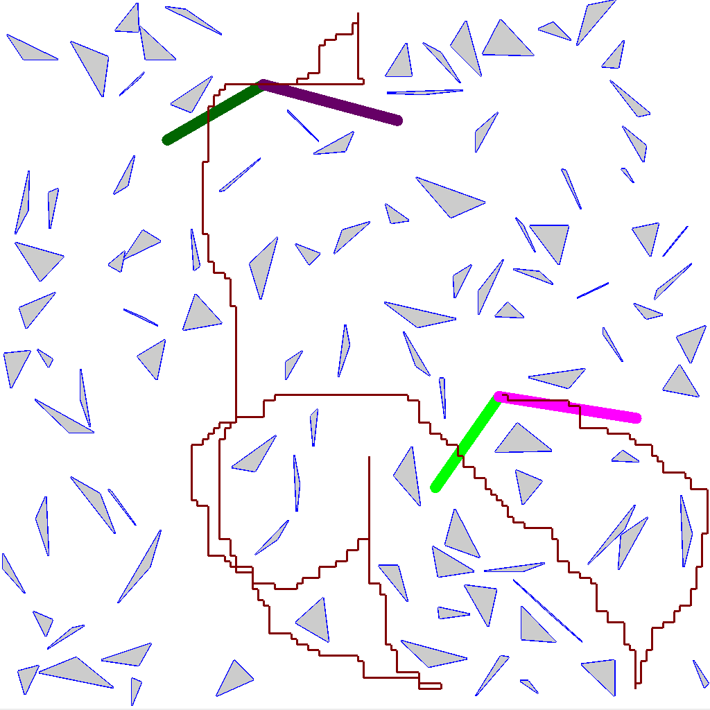
(a) Trace of robot origin

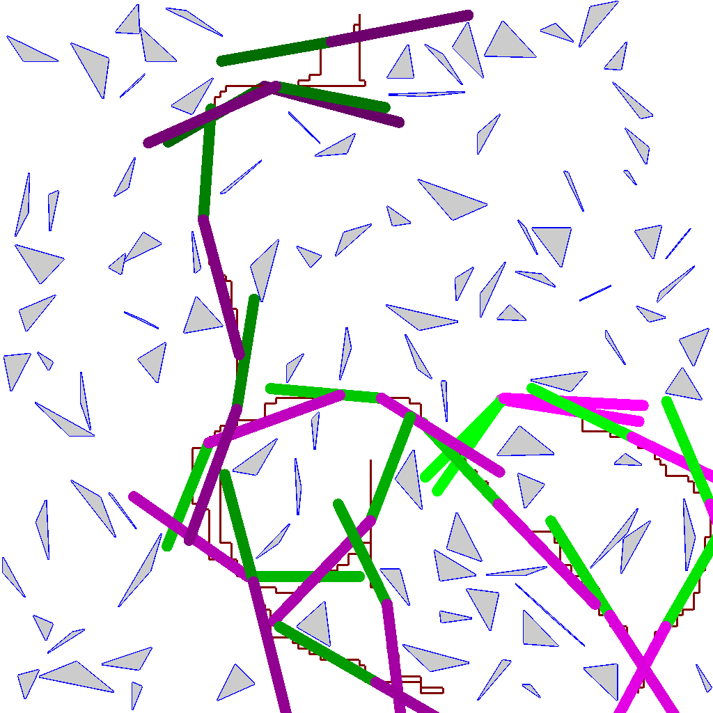
(b) Sub-sampled path

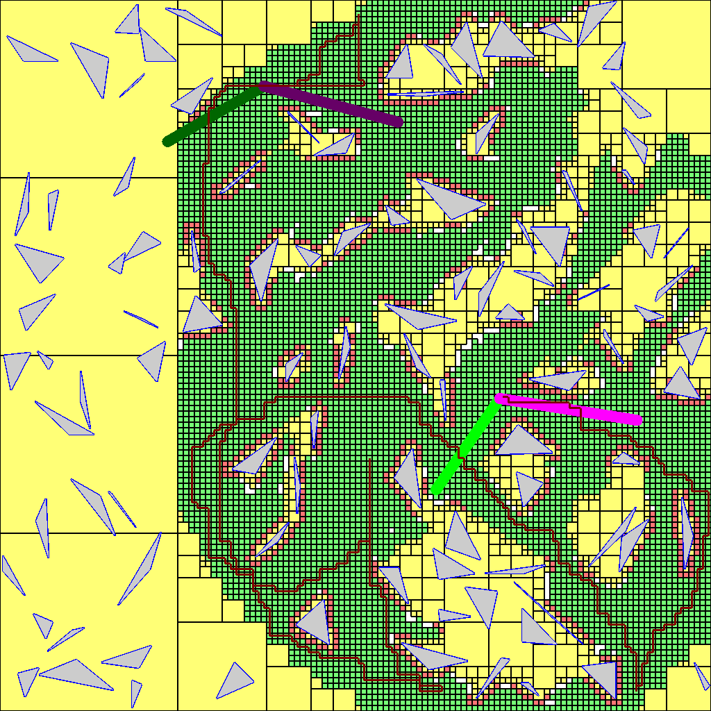
(c) Subdivision boxes

Figure 1: 100 Random Triangles Environment: non-crossing path found $(\kappa=115^{\circ})$

Link robots offer a compelling class of non-trivial robots for exploring path planning (see [6, chap. 7]). In the plane, the simplest example of a non-rigid robot is the 2-link robot, $R_{2}=R_{2}(\ell_{1},\ell_{2})$, with links of lengths $\ell_{1},\ell_{2}>0$. The two links are connected through a rotational joint $A_{0}$ called the robot origin. The 2-link robot is in the intersection of two well-known families of link robots, chain robots and spider robots (see [11]). One limitation of link robots is that links are unrealistically modeled by line segments. On the other hand, a model of mechanical links involving complex details may require algorithms that currently do not exist or have high computational complexity. As a compromise, we introduce thick links by forming the Minkowski sum of each link with a ball of radius $\tau>0$ (thin links correspond to $\tau=0$). To our knowledge, no exact algorithm for thick $R_{2}$ is known; for a single link $R_{1}$, an exact algorithm based on retraction follows from [14]. In this paper, we further parametrize $R_{2}$ by a “bandwidth” $\kappa$ which constrains the angle between the 2 links to be greater than or equal to $\kappa$ (“self-crossing” links is recovered by setting $\kappa<0$). Thus, our full robot model

$$R_{2}(\ell_{1},\ell_{2},\tau,\kappa)$$

has four parameters; our algorithms are uniform in these parameters.

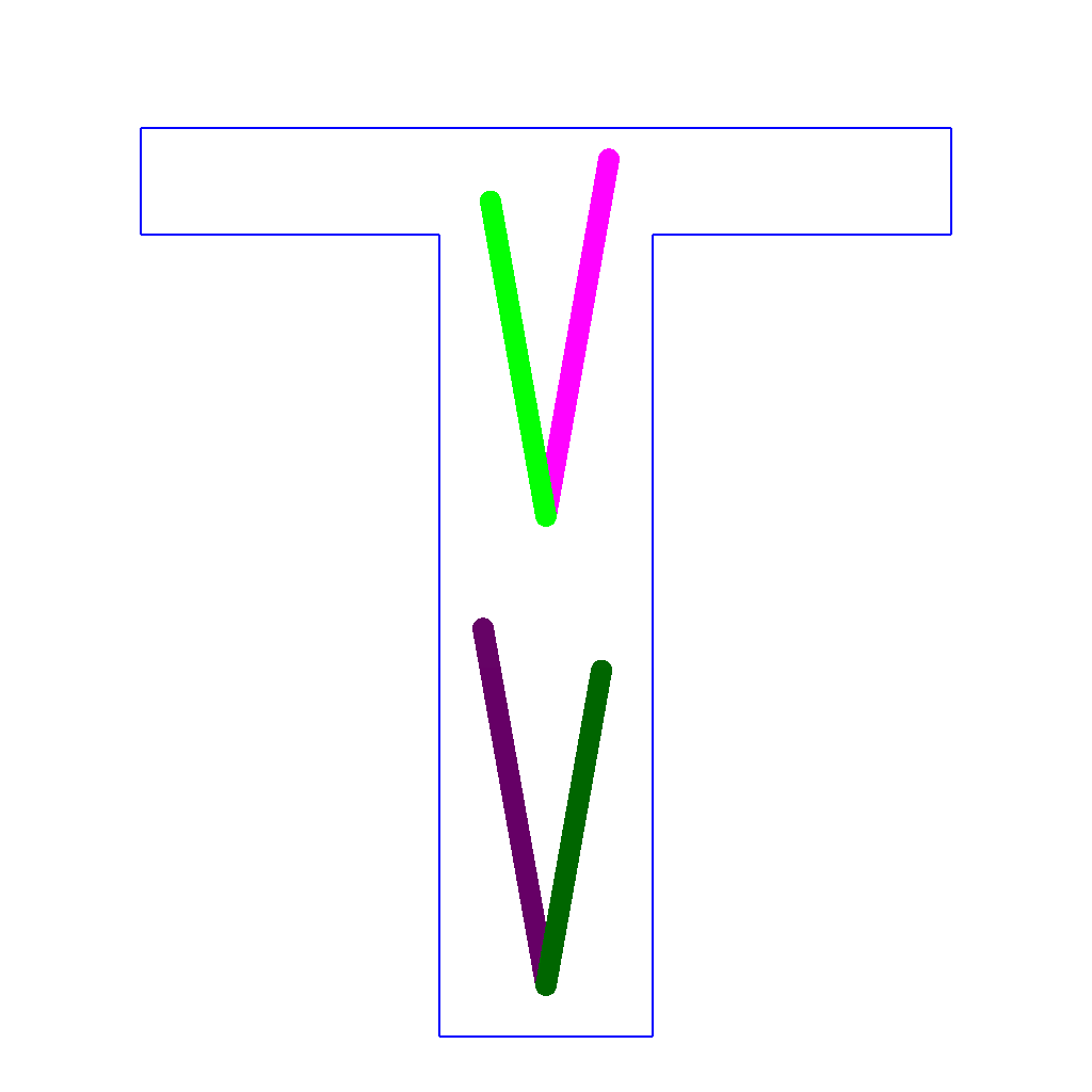
(a) $\alpha$ (above), $\beta$ (below)

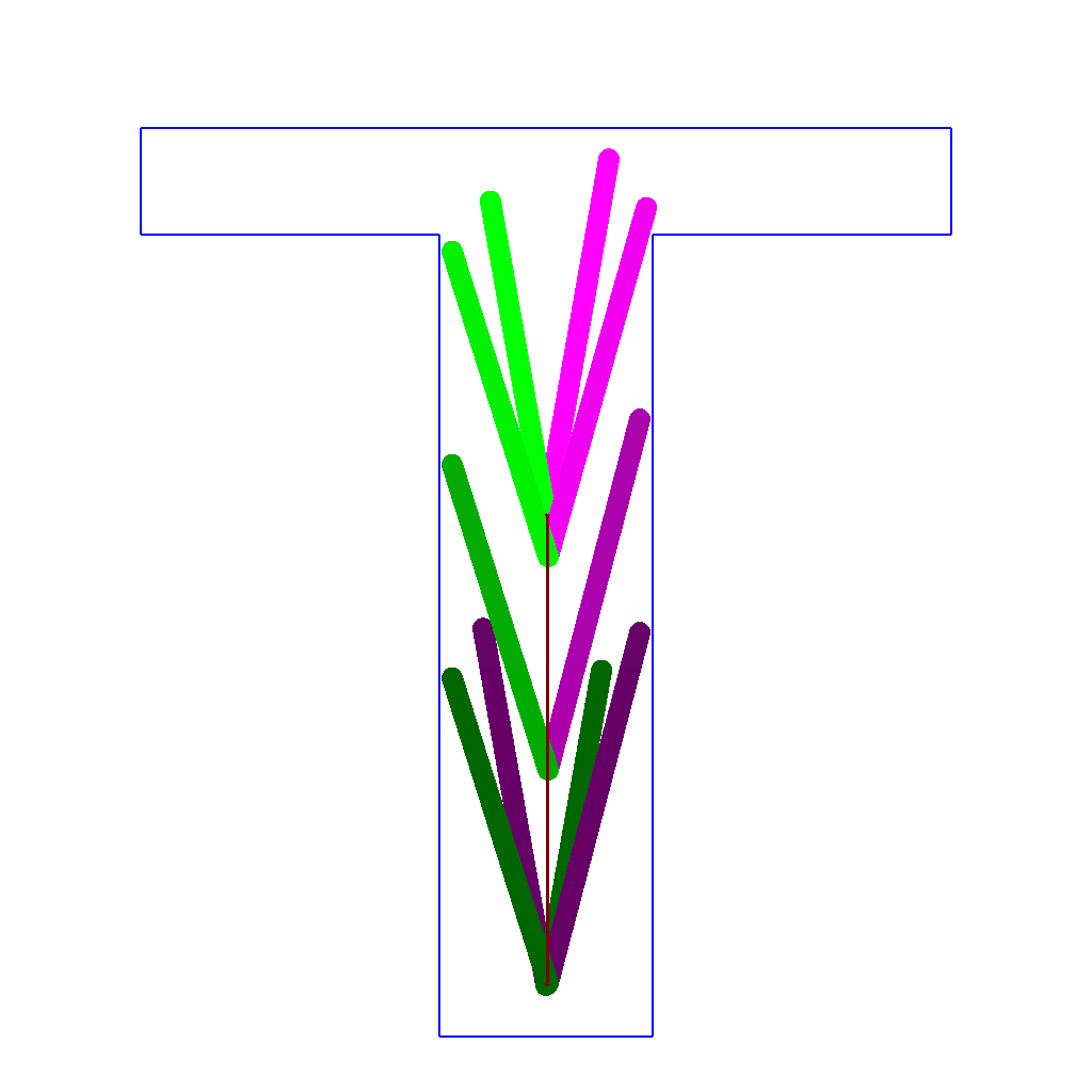
(b) Self-crossing path

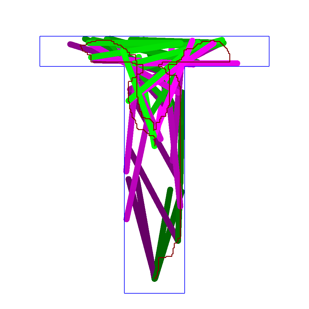
(c) Non-crossing path

Figure 2: Path from configurations $\alpha$ to $\beta$ in T-Room Environment

To illustrate the non-crossing constraint, we use the simple “T-room” environment in Figure 2. Suppose the robot has to move from the start configuration $\alpha$ to the goal configuration $\beta$ as indicated in Figure 2(a). There is an obvious path from $\alpha$ to $\beta$ as illustrated in Figure 2(b): the robot origin moves directly from its start to goal positions, while the link angles simultaneously adjust to their goal angles. However, such paths require the two links to cross each other. To achieve a “non-crossing” solution from $\alpha$ to $\beta$, we need a less obvious path such as found by our algorithm in Figure 2(c): the robot origin must first move away from the goal, towards the T-junction, in order to maneuver the 2 links into an appropriate relative order before moving toward the goal configuration.

We had chosen $\varepsilon=2$ in Figure 2(b,c); also, $\kappa$ is $7$ for the non-crossing instance. But if we increase either $\varepsilon$ to $3$ or $\kappa$ to $8$, then the non-crossing instance would report NO-PATH. It is important to know that the NO-PATH output from resolution-exact algorithms is not never due to exhaustion (“time-out”). It is a principled answer, guaranteeing the non-existence of paths with clearance $>K\cdot\varepsilon$ (for some $K>1$ depending on the algorithm). In our view, the narrow passage problem is, in the limit, just the halting problem for path planning: algorithms with narrow passage problems will also have non-halting issues when there is no path. Our experiments suggests that the “narrow passage problem” is barely an issue for our particular 4DOF robot, but it could be a severe issue for sampling approaches. But no amount of experimental data can truly express the conceptual gap between the various sampling heuristics and the a priori guaranteed methods such as ours.

Literature Review. Our theory of resolution-exactness and SSS algorithms apply to any robot system but we focus on algorithmic techniques to achieve the best algorithms for a 2-link robot. The main competition is from sampling approaches – see [3] for a survey. In our experiments, we compare against the well-known PRM [7] as well as variants such as Toggle PRM [4] and lazy version [5]. Another important family of sampling methods is the RRT with variants such as RRT-connect [8] and retraction-RRT [12]. The latter is comparable to Toggle PRM’s exploitation of non-free configurations, except that retraction-RRT focuses on contact configurations. Salzman et al [13] introduce a “tiling technique” for handling non-crossing links in sampling algorithms that is quite different from our subdivision solution [11].

Overview of Paper. Section 2 describes our parametrization of the configuration space of $R_{2}$, and implicitly, its free space. Section 3 analyzes the forbidden angles of thick links. Section 4 shows our subdivision representation of the non-crossing configuration space. Section 5 describes our experimental results. Section 6 concludes the paper. Omitted proofs and additional experimental data are available as appendices in the full paper [17].

2 Configuration Space of Non-Crossing 2-Link Robot

The configuration space of $R_{2}$ is $C_{space}\mathrel{:=}{\mathbb{R}}^{2}\times{\mathbb{T}}^{2}$ where ${\mathbb{T}}^{2}=S^{1}\times S^{1}$ is the torus and $S^{1}=SO(2)$ is the unit circle. We represent $S^{1}$ by the interval $[0,2\pi]$ with the identification $0=2\pi$. Closed angular intervals of $S^{1}$ are denoted by $[s,t]$ where $s,t\in[0,2\pi]$ using the convention

$$[s,t]\mathrel{:=}\left\{\begin{array}[]{lllllllllllllllllllllllll}\ \left\{\theta:s\leq\theta\leq t\right\}&\mbox{\rm\ if }\ s\leq t,\\ \ [s,2\pi]\cup[0,t]&\mbox{\rm\ if }\ s>t.\end{array}\right.$$

In particular, $[0,2\pi]=S^{1}$ and $[2\pi,0]=[0,0]$. The standard Riemannian metric $d:S^{1}\times S^{1}\to{\mathbb{R}}_{\geq 0}$ on $S^{1}$ is given by $d(\theta,\theta^{\prime})=\min\left\{|\theta-\theta^{\prime}|,2\pi-|\theta-\theta^{\prime}|\right\}$. Thus $0\leq d(\theta,\theta^{\prime})\leq\pi$.

To represent the non-crossing configuration space, we must be more specific about interpreting the parameters in a configuration $(x,y,\theta_{1},\theta_{2})\in C_{space}$: there are two distinct interpretations, depending on whether $R_{2}$ is viewed as a chain robot or a spider robot. We choose the latter view: then $(x,y)$ is the footprint of the joint $A_{0}$ at the center of the spider and $\theta_{1},\theta_{2}$ are the independent angles of the two links. This has some clear advantage over viewing $R_{2}$ as a chain robot, but we can conceive of other advantages for the chain robot view. That will be future research. In the terminology of [11], the robot $R_{2}$ has three named points $A_{0},A_{1},A_{2}$ whose footprints at configuration $\gamma=(x,y,\theta_{1},\theta_{2})$ are given by

$$A_{0}[\gamma]\mathrel{:=}(x,y),\quad A_{1}[\gamma]\mathrel{:=}(x,y)+\ell_{1}(\cos\theta_{1},\sin\theta_{1}),\quad A_{2}[\gamma]\mathrel{:=}(x,y)+\ell_{2}(\cos\theta_{2},\sin\theta_{2}).$$

The thin footprint of $R_{2}$ at $\gamma$, denoted $R_{2}[\gamma]$, is defined as the union of the line segments $[A_{0}[\gamma],A_{1}[\gamma]]$ and $[A_{0}[\gamma],A_{2}[\gamma]]$. The thick footprint of $R_{2}$ is given by $Fprint_{\tau}(\gamma)\mathrel{:=}D(\mbox{\bf 0},\tau)\oplus R_{2}[\gamma]$, the Minkowski sum $\oplus$ of the thin footprint with disc $D(\mbox{\bf 0},\tau)$ of radius $\tau$ centered at 0.

The non-crossing configuration space of bandwidth $\kappa$ is defined to be

$$C_{space}(\kappa)\mathrel{:=}{\mathbb{R}}^{2}\times({\mathbb{T}}^{2}\setminus\Delta(\kappa))$$

where $\Delta(\kappa)$ is the diagonal band $\Delta(\kappa)\mathrel{:=}\left\{(\theta,\theta^{\prime})\in{\mathbb{T}}^{2}:d(\theta,\theta^{\prime})\leq\kappa\right\}\subseteq{\mathbb{T}}^{2}.$ Note three special cases:

• If $\kappa<0$ then $\Delta(\kappa)$ is the empty set.

• If $\kappa=0$ then $\Delta(\kappa)$ is a closed curve in ${\mathbb{T}}^{2}$.

• If $\kappa\geq\pi$ then $\Delta(\kappa)=S^{1}$.

Configurations in ${\mathbb{R}}^{2}\times\Delta(0)$ are said to be self-crossing; all other configurations are non-crossing. Here we focus on the case $\kappa\geq 0$. For our subdivision below, we will split ${\mathbb{T}}^{2}\setminus\Delta(0)$ into two connected sets: ${\mathbb{T}}^{2}_{<}\mathrel{:=}\left\{(\theta,\theta^{\prime})\in{\mathbb{T}}^{2}:0\leq\theta<\theta^{\prime}<2\pi\right\}$ and ${\mathbb{T}}^{2}_{>}\mathrel{:=}\left\{(\theta,\theta^{\prime})\in{\mathbb{T}}^{2}:0\leq\theta^{\prime}<\theta<2\pi\right\}$. For $\kappa\geq 0$, the diagonal band $\Delta(\kappa)$ retracts to the closed curve $\Delta(0)$. In ${\mathbb{R}}^{2}$, if we omit such a set, we will get two connected components. In contrast, that ${\mathbb{T}}^{2}\setminus\Delta(\kappa)$ remains connected. CLAIM: ${\mathbb{T}}^{2}\setminus\Delta(\kappa)$ is topologically a cylinder with two boundary components. Thus, the non-crossing constraint has changed the topology of the configuration space. To see claim, consider the standard model of ${\mathbb{T}}^{2}$ represented by a square with opposite sides identified as in Figure 3(a) (we show the case $\kappa=0$). By rearranging the two triangles ${\mathbb{T}}^{2}_{<}$ and ${\mathbb{T}}^{2}_{>}$ as in Figure 3(b), our claim is now visually obvious.

Figure 3: Paths in ${\mathbb{T}}^{2}\setminus\Delta(0)$ from $\alpha\in{\mathbb{T}}^{2}_{>}$ to $\beta\in{\mathbb{T}}^{2}_{<}$

3 Forbidden Angle Analysis of Thick Links

Towards the development of a soft-predicate for thick links, we must first extend our analysis in [11] which introduced the concept of forbidden angles for thin links. Let $L(\ell,\tau)$ be a single link robot of length $\ell>0$ and thickness $\tau\geq 0$. Its configuration space is $SE(2)={\mathbb{R}}^{2}\times S^{1}$. Given a configuration $(b,\theta)\in SE(2)$, the footprint of $L(\ell,\tau)$ at $(b,\theta)$ is

$$Fprint_{\ell,\tau}(b,\theta)\mathrel{:=}L\oplus D(\mbox{\bf 0},\tau)$$

where $\oplus$ denotes Minkowski sum, $L$ is the line segment $[b,b+\ell(\cos\theta,\sin\theta)]$ and $D(\mbox{\bf 0},\tau)$ is the disk as above. When $\ell,\tau$ is understood, we simply write “$Fprint(b,\theta)$” instead of $Fprint_{\ell,\tau}(b,\theta)$.

Let $S,T\subseteq{\mathbb{R}}^{2}$ be closed sets. An angle $\theta$ is forbidden for $(S,T)$ if there exists $s\in S$ such that $Fprint(s,\theta)\cap T$ is non-empty. If $t\in Fprint(s,\theta)\cap T$, then the pair $(s,t)\in S\times T$ is a witness for the forbidden-ness of $\theta$ for $(S,T)$. The set of forbidden angles of $(S,T)$ is called the forbidden zone of $S,T$ and denoted $\mathrm{Forb}_{\ell,\tau}(S,T)$. Clearly, $\theta\in\mathrm{Forb}_{\ell,\tau}(S,T)$ iff there exists a witness pair $(s,t)\in S\times T$. Moreover, we call $(s,t)$ a minimum witness of $\theta$ if the Euclidean norm $\|s-t\|$ is minimum among all witnesses of $\theta$. If $(s,t)$ is a minimum witness, then clearly $s\in\partial S$ and $t\in\partial T$.

Lemma 1

For any sets $S,T\subseteq{\mathbb{R}}^{2}$, we have

$$\mathrm{Forb}_{\ell,\tau}(S,T)=\pi+\mathrm{Forb}_{\ell,\tau}(T,S).$$

Proof. For any pair $(s,t)$ and any angle $\alpha$, we see that

$$t\in Fprint(s,\alpha)\mbox{\rm\ iff }\ s\in Fprint(t,\pi+\alpha).$$

Thus, there is a witness $(s,t)$ for $\alpha$ in $\mathrm{Forb}_{\ell,\tau}(S,T)$ iff there is a witness $(t,s)$ for $\pi+\alpha$ in $\mathrm{Forb}_{\ell,\tau}(T,S)$. The lemma follows.   Q.E.D.

¶1. The Forbidden Zone of two points Consider the forbidden zone $\mathrm{Forb}_{\ell,\tau}(V,C)$ defined by two points $V,C\in{\mathbb{R}}^{2}$ with $d=\|V-C\|$. (The notation $V$ suggests a vertex of a translational box $B^{t}$ and $C$ suggests a corner of the obstacle set.) In our previous paper [11] on thin links (i.e., $\tau=0$), this case is not discussed for reasons of triviality. When $\tau>0$, the set $\mathrm{Forb}_{\ell,\tau}(V,C)$ is more interesting. Clearly, $\mathrm{Forb}_{\ell,\tau}(V,C)$ is empty iff $d>\ell+\tau$ (and a singleton if $d=\ell+\tau$). Also $\mathrm{Forb}_{\ell,\tau}(V,C)=S^{1}$ iff $d\leq\tau$. Henceforth, we may assume

$$\tau<d<\ell+\tau.$$ (1)

The forbidden zone of $V,C$ can be written in the form

$$\mathrm{Forb}_{\ell,\tau}(V,C)\mathrel{:=}[\nu-\delta,\nu+\delta]$$

for some $\nu,\delta$. Call $\nu$ the nominal angle and $\delta$ the correction angle. By the symmetry of the footprint, $\nu$ is equal to $\theta(V,C)$ (see Figure 4).

Figure 4: $\mathrm{Forb}_{\ell,\tau}(V,C)$

It remains to determine $\delta$. Consider the configuration $(V,\theta)\in SE(2)$ of our link $L(\ell,\tau)$ where link origin is at $V$ and the link makes an angle $\theta$ with the positive $x$-axis. The angle $\delta$ is determined when the point $C$ lies on the boundary of $Fprint(V,\theta)$. The two cases are illustrated in Figure 4 where $\theta=\nu+\delta$ and other endpoint of the link is $U$; thus $\|VU\|=\ell$ and $\|VC\|=d$, and $\delta=\angle(CVU)$. Under the constraint (1), there are two ranges for $d$:

1. $d$ is short: $d^{2}\leq\tau^{2}+\ell^{2}$. In this case, the point $C$ lies on the straight portion of the boundary of the footprint, as in Figure 4(a). From the right-angle triangle $CU^{\prime}V$, we see that $\delta=\arcsin(\tau/d)$.

2. $d$ is long: $d^{2}>\tau^{2}+\ell^{2}$. In this case, the point $C$ lies on the circular portion of the boundary of the footprint, as in Figure 4(b). Consider the triangle $CUV$ with side lengths of $d,\ell,\tau$. By the cosine law, $\tau^{2}=d^{2}+\ell^{2}-2d\ell\cos\delta$ and thus

   $$\delta=\arccos\left({\frac{\ell^{2}+d^{2}-\tau^{2}}{2d\ell}}\right).$$

This proves:

Lemma 2

Assume $\|VC\|=d$ satisfies (1). Then

$$\mathrm{Forb}_{\ell,\tau}(V,C)=[\nu-\delta,\nu+\delta]$$

where $\nu=\theta(V,C)$ and

$$\delta=\delta(V,C)=\left\{\begin{array}[]{lllllllllllllllllllllllll}\arcsin(\tau/d)&\mbox{\rm\ if }\ d^{2}\leq\tau^{2}+\ell^{2},\\ \arccos\left({\frac{\ell^{2}+d^{2}-\tau^{2}}{2d\ell}}\right)&\mbox{\rm\ if }\ d^{2}>\tau^{2}+\ell^{2}.\end{array}\right.$$ (2)

¶2. The Forbidden Zone of a Vertex and a Wall Recall that the boundary of a box $B^{t}$ is divided into four sides, and two adjacent sides share a common endpoint which we call a vertex. We now determine $\mathrm{Forb}_{\ell,\tau}(V,W)$ where $V$ is a vertex and $W$ a wall feature. Choose the coordinate axes such that $W$ lies on the $x$-axis, and $V=(0,-\sigma)$ lies on the negative $y$-axis, for some $\sigma>0$. Let the two corners of $W$ be $C,C^{\prime}$ with $C^{\prime}$ lying to the left of $C$. See Figure 5.

Figure 5: Stop Analysis for $\mathrm{Forb}_{\ell,\tau}(V,W)$ (assuming $\sigma>\tau$)

We first show that the interesting case is when

$$\tau<\sigma<\ell+\tau.$$ (3)

If $\sigma\geq\ell+\tau$ then $\mathrm{Forb}_{\ell,\tau}(V,W)$ is either a singleton ($\sigma=\ell+\tau$) or else is empty ($\sigma>\ell+\tau$). Likewise, the following lemma shows that when $\sigma\leq\tau$, we are to point-point case of Lemma 2:

Lemma 3

Assume $\sigma\leq\tau$. We have

$$\mathrm{Forb}_{\ell,\tau}(V,W)=\left\{\begin{array}[]{lllllllllllllllllllllllll}S^{1}&\mbox{\rm\ if }\ D(V,\tau)\cap W\neq\emptyset,\\ \mathrm{Forb}_{\ell,\tau}(V,c)&\mbox{\rm\ else}\end{array}\right.$$

where $c=C$ or $C^{\prime}$.

Proof. Recall that we have chosen the coordinate system so that $W$ lies on the $x$-axes and $V=(0,-\sigma)$. It is easy to see that $\mathrm{Forb}_{\ell,\tau}(V,W)=S^{1}$ iff the disc $D(V,\tau)$ intersects $W$. So assume otherwise. In that case, the closest point in $W$ to $V$ is $c$, one of the two corners of $W$. The lemma is proved if we show that

$$\mathrm{Forb}_{\ell,\tau}(V,W)=\mathrm{Forb}_{\ell,\tau}(V,c).$$

It suffices to show $\mathrm{Forb}_{\ell,\tau}(V,W)\subseteq\mathrm{Forb}_{\ell,\tau}(V,c)$. Suppose $\theta\in\mathrm{Forb}_{\ell,\tau}(V,W)$. So it has a witness $(V,c^{\prime})$ for some $c^{\prime}\in W$. However, we see that the minimal witness for this case is $(V,c)$. This proves that $\theta\in\mathrm{Forb}_{\ell,\tau}(V,c)$.   Q.E.D.

In addition to (3), we may also assume the wall lies within the annulus of radii $(\tau,\tau+\ell)$ centered at $V$:

$$\|VC\|,\|VC^{\prime}\|\in(\tau,\ell+\tau)$$ (4)

Using the fact that $V=(0,-\sigma)$ and $W$ lies in the $x$-axis, we have:

Lemma 4

Assume (3) and (4).
Then $\mathrm{Forb}_{\ell,\tau}(V,W)$ is a non-empty connected interval of $S^{1}$,

$$\mathrm{Forb}_{\ell,\tau}(V,W)=[\alpha,\beta]\subseteq(0,\pi).$$

Our next goal is to determine the angles $\alpha,\beta$ in this lemma. Consider the footprints of the link at the extreme configurations $(V,\alpha),(V,\beta)\in SE(2)$. Clearly, $W$ intersects the boundary (but not interior) of these footprints, $Fprint(V,\alpha)$ and $Fprint(V,\beta)$. Except for some special configurations, these intersections are singleton sets. Regardless, pick any $A\in W\cap Fprint(V,\alpha)$ and $B\in W\cap Fprint(V,\beta)$. Since $\alpha$ is an endpoint of $\mathrm{Forb}_{\ell,\tau}(V,W)$, we see that $A\in(\partial W)\cap\partial(Fprint(V,\alpha))$. We call $A$ a left stop for the pair $(V,W)$ because for any $\delta^{\prime}>0$ small enough, $A\in Fprint(V,\alpha+\delta^{\prime})$ while $W\cap(V,\alpha-\delta^{\prime})=\emptyset$. Similarly the point $B$ is called a right stop for the pair $(V,W)$. Clearly, we can write

$$\alpha=\theta(V,A)-\delta(V,A),\qquad\beta=\theta(V,B)+\delta(V,B)$$

where $\delta(V,\cdot)$ is given by Lemma 2. We have thus reduced the determination of angles $\alpha$ and $\beta$ to the computation of the left $A$ and right $B$ stops.

We might initially guess that the left stop of $(V,W)$ is $C$, and right stop of $(V,W)$ is $C^{\prime}$. But the truth is a bit more subtle. Define the following points $X_{*},X_{\max}$ on the positive $x$-axis using the equation:

$$\|OX_{*}\| = \sqrt{(\ell+\tau)^{2}-\sigma^{2}},$$

$$\|OX_{\max}\| = \sqrt{\ell^{2}-(\sigma-\tau)^{2}}.$$

These two points are illustrated in Figure 5. Also, let $\overline{X}_{*}$ and $\overline{X}_{\max}$ be mirror reflections of $X_{*}$ and $X_{\max}$ across the $y$-axis. The points $X_{*},\overline{X}_{*}$ are the two points at distance $\ell+\tau$ from $V$. The points $X_{\max},\overline{X}_{\max}$ are the left and right stops in we replace $W$ by the infinite line through $W$ (i.e., the $x$-axis).

With the natural ordering of points on the $x$-axis, we can show that

$$\overline{X}_{*}<\overline{X}_{\max}<O<X_{\max}<X_{*}$$

where $O$ is the origin. Since $\|VC\|$ and $\|VC^{\prime}\|$ lie in $(\tau,\tau+\ell)$, it follows that

$$\overline{X}_{*}<C^{\prime}<C<X_{*}.$$

Two situations are shown in Figure 5. The next lemma is essentially routine, once the points $X_{\max},\overline{X}_{\max}$ have defined:

Lemma 5

Assume (3) and (4).
The left stop of $(V,W)$ is

$$\left\{\begin{array}[]{lllllllllllllllllllllllll}C^{\prime}&\mbox{\rm\ if }\ X_{\max}\leq C^{\prime}&\qquad(L1)\\ X_{\max}&\mbox{\rm\ if }\ C^{\prime}<X_{\max}<C&\qquad(L2)\\ C&\mbox{\rm\ if }\ C\leq X_{\max}&\qquad(L3)\end{array}\right.$$

The right stop of $(V,W)$ is

$$\left\{\begin{array}[]{lllllllllllllllllllllllll}C&\mbox{\rm\ if }\ C\leq\overline{X}_{\max}&\qquad(R1)\\ \overline{X}_{\max}&\mbox{\rm\ if }\ C^{\prime}<\overline{X}_{\max}<C&\qquad(R2)\\ C^{\prime}&\mbox{\rm\ if }\ \overline{X}_{\max}\leq C^{\prime}&\qquad(R3)\end{array}\right.$$

The cases (L1-3) and (R1-3) in this lemma suggests 9 combinations, but 3 are logically impossible: (L1-R1), (L1-R2), (L2-R1). The remaining 6 possibilities for left and right stops are summarized in the following table:

	(R1)	(R2)	(R3)
(L1)	*	*	$~{}(C^{\prime},C^{\prime})~{}$
(L2)	*	$~{}(X_{\max},\overline{X}_{\max})~{}$	$~{}(X_{\max},C^{\prime})~{}$
(L3)	$~{}(C,C)~{}$	$~{}(C,\overline{X}_{\max})~{}$	$~{}(C,C^{\prime})~{}$

Observe the extreme situations (L1-R3) or (L3-R1) where the the left and right stops are equal to the same corner, and we are reduced to the point-point analysis. Once we know the left and right stops for $(V,W)$, then we can use Lemma 2 to calculate the angles $\alpha$ and $\beta$.

¶3. The Forbidden Zone of a Side and a Corner We now consider the forbidden zone $\mathrm{Forb}_{\ell,\tau}(S,C)$ where $S$ is a side and $C$ a corner feature. Note that is complementary to the previous case of $\mathrm{Forb}_{\ell,\tau}(V,W)$ since $C$ and $V$ are points and $S$ and $W$ are line segments. We can exploit the principle of reflection symmetry of Lemma 1:

$$\mathrm{Forb}_{\ell,\tau}(S,C)=\pi+\mathrm{Forb}_{\ell,\tau}(C,S)$$

where $\mathrm{Forb}_{\ell,\tau}(C,S)$ is provided by previous Lemma (with $C,S$ instead of $V,W$).

¶4. Cone Decomposition We have now provided formulas for computing sets of the form $\mathrm{Forb}_{\ell,\tau}(V,W)$ or $\mathrm{Forb}_{\ell,\tau}(S,C)$; such sets are called cones. We now address the problem of computing $\mathrm{Forb}_{\ell,\tau}(B^{t},W)$ where $B^{t}\subseteq{\mathbb{R}}^{2}$ is a (translational) box. We show that this set of forbidden angles can be written as the union of at most 3 cones, generalizes a similar result in [11]. Towards such a cone decomposition, we first classify the disposition of a wall $W$ relative to a box $B^{t}$. There is a preliminary case: if $W$ intersects $B^{t}\oplus D(0,\tau)$, then we have

$$\mathrm{Forb}_{\ell}(B^{t},W)=S^{1}.$$

Call this Case (0). Assuming $W$ does not intersect $B^{t}\oplus D(0,\tau)$, there are three other possibilities, Cases (I-III) illustrated Figure 6.

Figure 6: Cases (I-III) of $\mathrm{Forb}_{\ell,\tau}(B^{t},W)$

We first need a notation: if $S\subseteq\partial(B^{t})$ is a side of the box $B^{t}$, let $H(S)$ denote the open half-space which is disjoint from $B^{t}$ and is bounded by the line through $S$. Then we have these three cases:

1. $W\subseteq H(S)$ for some side $s$ of box $B^{t}$.

2. $W\subseteq H(S)\cap H(S^{\prime})$ for two adjacent sides $S,S^{\prime}$ of box $B^{t}$.

3. None of the above. This implies that $W\subseteq H(S)\cup H(S^{\prime})$ for two adjacent sides $S,S^{\prime}$ of box $B^{t}$.

Theorem 3.1

$\mathrm{Forb}_{\ell,\tau}(B^{t},W)$ is the union of at most three thick cones.

Sketch proof: we try to reduce the argument to the case $\tau=0$ which is given in [11]. In that case, we could write

$$\mathrm{Forb}_{\ell}(B^{t},W)=C_{1}\cup C_{2}\cup C_{3}$$

where each $C_{i}$ is a thin cone or an empty set. In the non-empty case, the cone $C_{i}$ has the form $\mathrm{Forb}_{\ell}(S_{i},T_{i})$ where $S_{i}\subseteq\partial B^{t},T_{i}\subseteq W$. The basic idea is that we now “transpose” $\mathrm{Forb}_{\ell}(S_{i},T_{i})$ to the thick version $C^{\prime}_{i}\mathrel{:=}\mathrm{Forb}_{\ell,\tau}(S_{i},T_{i})$. In case $C_{i}$ is empty, $C^{\prime}_{i}$ remains empty. Thus we would like to claim that

$$\mathrm{Forb}_{\ell}(B^{t},W)=C^{\prime}_{1}\cup C^{\prime}_{2}\cup C^{\prime}_{3}.$$

This is almost correct, except for one issue. It is possible that some $C_{i}$ is empty, and yet its transpose $C^{\prime}_{i}$ is non empty. See proof in the full paper [17]. In case of thin cones, the $C_{i}$’s are non-overlapping (i.e., they may only share endpoints). But for thick cone decomposition, the cones will in general overlap.

4 Subdivision for Thick Non-Crossing 2-Link Robot

A resolution-exact planner for a thin self-crossing 2-link robot was described in [11]. We now extend that planner to the thick non-crossing case.

We will briefly review the ideas of the algorithm for the thin self-crossing 2-link robot. We begin with a box $B_{0}\subseteq{\mathbb{R}}^{2}$ and it is in the subspace $B_{0}\times{\mathbb{T}}^{2}\subseteq C_{space}$ where our planning problem takes place. We are also given a polygonal obstacle set $\Omega\subseteq{\mathbb{R}}^{2}$; we may decompose its boundary $\partial\Omega$ into a disjoint union of corners (=points) and edges (=open line segments) which are called (boundary) features. Let $B\subseteq C_{space}$ be a box; there is an exact classification of $B$ as $C(B)\in\left\{\mathtt{FREE},\mathtt{STUCK},\mathtt{MIXED}\right\}$ relative to $\Omega$. But we want a soft classification $\widetilde{C}(B)$ which is correct whenever $\widetilde{C}(B)\neq\mathtt{MIXED}$, and which is equal to $C(B)$ when the width of $B$ is small enough. Our method of computing $\widetilde{C}(B)$ is based on computing a set $\phi(B)$ of features that are relevant to $B$. A box $B\subseteq C_{space}$ may be written as a Cartesian product $B=B^{t}\times B^{r}$ of its translational subbox $B^{t}\subseteq{\mathbb{R}}^{2}$ and rotational subbox $B^{r}\subseteq{\mathbb{T}}^{2}$. In the T/R splitting method (simple version), we split $B^{t}$ until the width of $B^{t}$ is $\leq\varepsilon$. Then we do a single split of the rotational subbox $B^{r}$ into all the subboxes obtained by removing all the forbidden angles determined by the walls and corners in $\widetilde{\phi}(B^{t})$. This “rotational split” of $B^{r}$ is determined by obstacles, unlike the “translational splits” of $B^{t}$.

¶5. Boxes for Non-Crossing Robot. Our basic idea for representing boxes in the non-crossing configuration space $C_{space}(\kappa)$ is to write it as a pair $(B,{\tt XT})$ where ${\tt XT}\in\left\{{\tt LT},{\tt GT}\right\}$, and $B\subseteq C_{space}$. The pair $(B,{\tt XT})$ represents the set $B\cap({\mathbb{R}}^{2}\times{\mathbb{T}}^{2}_{\tt XT})$ (with the identification ${\mathbb{T}}^{2}_{\tt LT}={\mathbb{T}}^{2}_{<}$ and ${\mathbb{T}}^{2}_{\tt GT}={\mathbb{T}}^{2}_{>}$). It is convenient to call $(B,{\tt XT})$ an $X$-box since they are no longer “boxes” in the usual sense.

An angular interval $\Theta\subseteq S^{1}$ that contains a open neighborhood of $0=2\pi$ is said to be wrapping. Also, call $B^{r}=\Theta_{1}\times\Theta_{2}$ wrapping if either $\Theta_{1}$ or $\Theta_{2}$ is wrapping. Given any $B^{r}$, we can decompose the set $B^{r}\cap({\mathbb{T}}^{2}\setminus\Delta(\kappa))$ into the union of two subsets $B^{r}_{\tt LT}$ and $B^{r}_{\tt GT}$, where $B^{r}_{\tt XT}$ denote the set $B^{r}\cap{\mathbb{T}}^{2}_{\tt XT}$. In case $B^{r}$ is non-wrapping, this decomposition has the nice property that each subset $B^{r}_{\tt XT}$ is connected. For this reason, we prefer to work with non-wrapping boxes. Initially, the box $B^{r}={\mathbb{T}}^{2}$ is wrapping. The initial split of ${\mathbb{T}}^{2}$ should be done in such a way that the children are all non-wrapping: the “natural” (quadtree-like) way to split ${\mathbb{T}}^{2}$ into four congruent children has this property. Thereafter, subsequent splitting of these non-wrapping boxes will remain non-wrapping.

Of course, $B^{r}_{\tt XT}$ might be empty, and this is easily checked: say $\Theta_{i}=[s_{i},t_{i}]$ ($i=1,2$). Then $B^{r}_{<}$ is empty iff $t_{2}\leq s_{1}$. and $B^{r}_{>}$ is empty iff $s_{2}\geq t_{1}$. Moreover, these two conditions are mutually exclusive.

We now modify the algorithm of [11] as follows: as long as we are just splitting boxes in the translational dimensions, there is no difference. When we decide to split the rotational dimensions, we use the T/R splitting method of [11], but each child is further split into two $X$-boxes annotated by ${\tt LT}$ or ${\tt GT}$ (they are filtered out if empty). We build the connectivity graph $G$ (see Appendix A) with these $X$-boxes as nodes. This ensures that we only find non-crossing paths. Our algorithm inherits resolution-exactness from the original self-crossing algorithm.

The predicate ${\tt isBoxEmpty}(B^{r},\kappa,{\tt XT})$ which returns true iff $(B^{r}_{\tt XT})\cap({\mathbb{T}}^{2}\setminus\Delta(\kappa))$ is empty is useful in implementation. It has a simple expression when restricted to non-wrapping translational box $B^{r}$:

Lemma 6

Let $B^{r}=[a,b]\times[a^{\prime},b^{\prime}]$ be a non-wrapping box.
(a) ${\tt isBoxEmpty}(B^{r},\kappa,{\tt LT})=\mbox{\tt true}$ iff $\kappa\geq b^{\prime}-a$ or $2\pi-\kappa\leq a^{\prime}-b$.
(b) ${\tt isBoxEmpty}(B^{r},\kappa,{\tt GT})=\mbox{\tt true}$ iff $\kappa\geq b-a^{\prime}$ or $2\pi-\kappa\leq a-b^{\prime}$.

5 Implementation and Experiments

We implemented our thick non-crossing 2-link planner in C++ and OpenGL on the Qt platform. A preliminary heuristic version appeared [11, 10]. Our code, data and experiments are distributed with our open source Core Library. To evaluate our planner, we compare it with several sampling algorithms in the open source OMPL [15]. Besides, based on a referee’s suggestion, we also implemented the 2-link (crossing and non-crossing) versions of Toggle PRM and Lazy Toggle PRM (in lieu of publicly available code). We benefited greatly from the advice of Prof. Denny in our best effort implementation. The machine we use is a MacBook Pro with 2.5 GHz Intel Core i7 and 16GB DDR3-1600 MHz RAM.

Tables 1 and 2 summarize the results of two groups of experiments, which we call Narrow Passages and Easy Passages. Each row in the tables represents an experiment, each column represents a planner. There are 8 planners: 3 versions of SSS, 3 versions of PRM and 2 versions of RRT. Only Table 1 is listed in the paper; Table 2 (as well as other experimental results) are relegated to an appendix. We extract two bar charts from Table 1 in Figure 7 for visualization to show the average times and success rates of the planners in Narrow Passages. Timing is in milliseconds on a Log10 scale. E.g., the bar chart Figure 7(a) for Narrow Passages shows that the average time for the SSS(I) planner in the T-Room experiment is about $2.9$. This represents $10^{2.9}\simeq 800$ milliseconds; indeed the actual value is $815.9$ as seen in Table 1. On this bar chart, each unit represents a power of 10. E.g., if one bar is at least $k$ units shorter than another bar, we say the former is “$k$ orders of magnitude” faster (i.e., at least $10^{k}$ times faster). Conclusion: (1) SSS is at least an order of magnitude faster than each sampling method, and (2) success rates of RRT-connect and Toggle PRM are usually (but not always) best among sampling methods, but both are inferior to SSS.

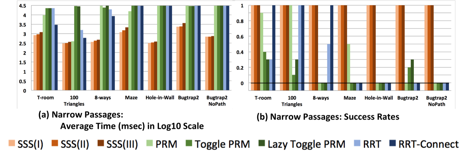
Figure 7: Bar Charts of Average Times and Success Rates

Two general remarks are in order. First, as in our previous work, we implemented several search strategies in SSS. But for simplicity, we only use the Greedy Best First (GBF) strategy in all the SSS experiments; GBF is typically our best strategy. Next, OMPL does not natively support articulated robots such as $R_{2}$. So in the experiments of Tables 1 and 2, we artificially set $\ell_{2}=0$ for all the sampling algorithms (so that they are effectively one-link thick robots). This is a suboptimal experimental scenario, but it only reinforces any exhibited superiority of our SSS methods. In the SSS versions, we set $\ell_{2}=0$ for SSS(I) but SSS(II) and SSS(III) represent (resp.) crossing and non-crossing 2-link robots where $\ell_{2}$ has the values shown in the column 4 header of Table 1.

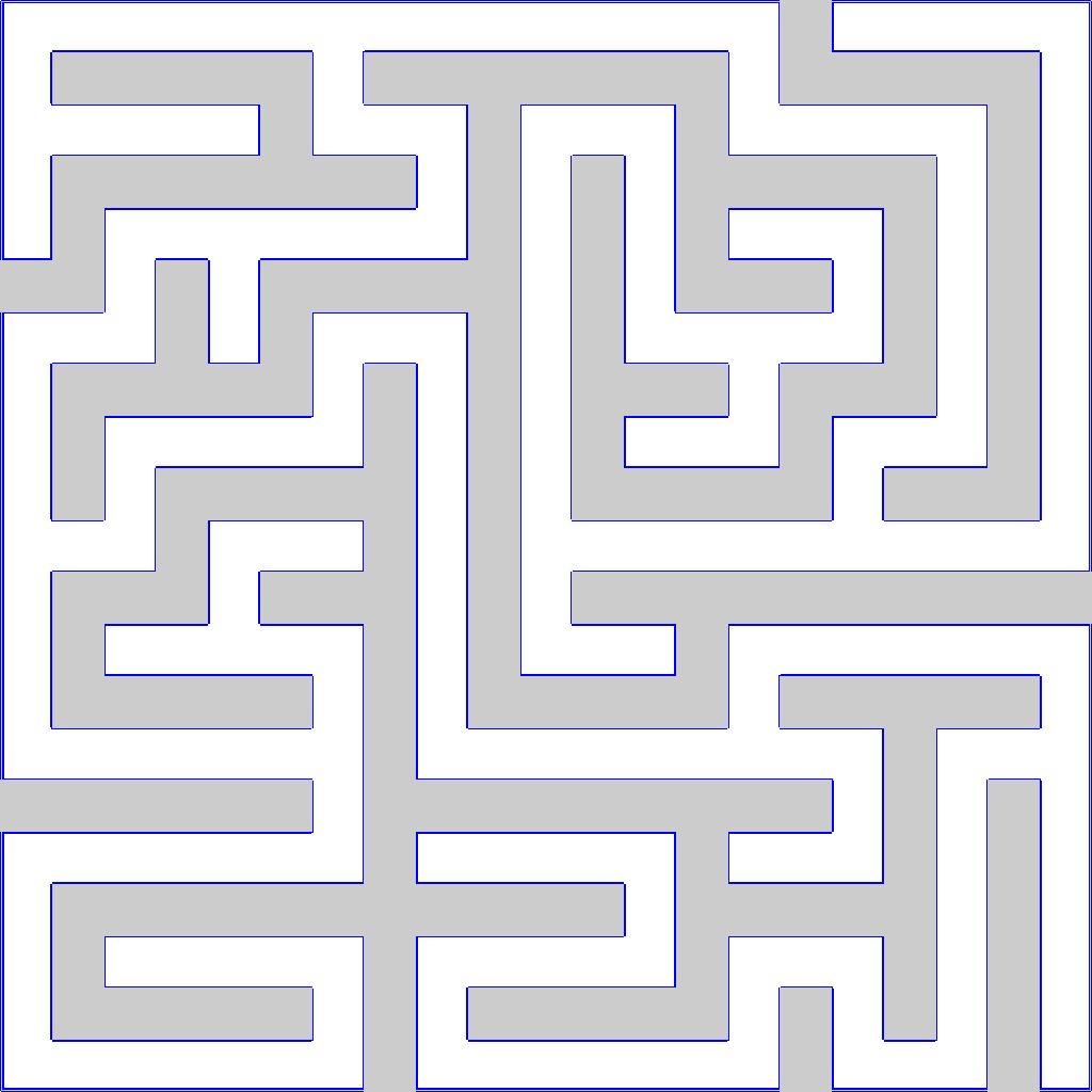
(a) Maze

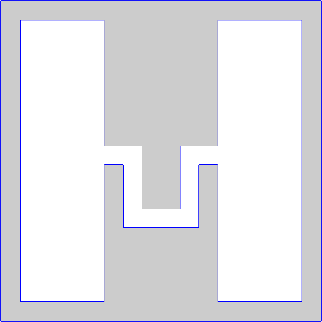
(b) Hole-in-Wall

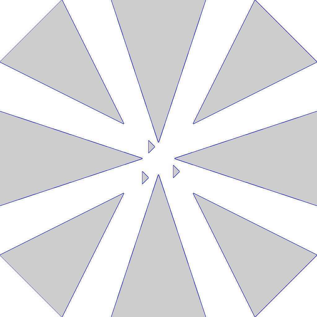
(c) 8-Way Corridor

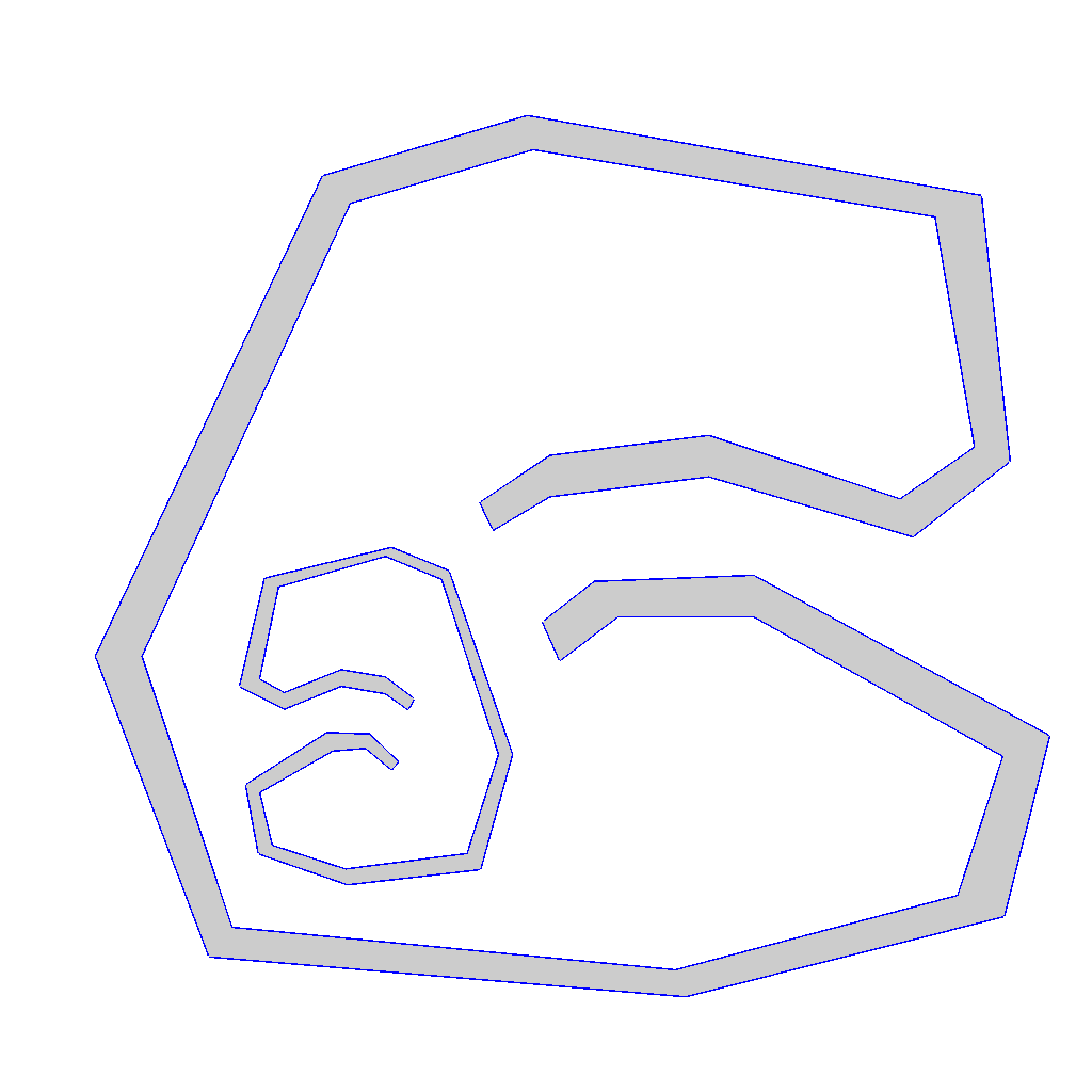
(d) Bugtrap2

Figure 8: More environments in our experiments

Reading the Tables: Each experiment (i.e., row) corresponds to a fixed environment, robot parameters, initial and goal configurations. Figure 8 depicts these environments (save for the T-Room and 100 triangles from the introduction). We name the experiments after the environment. E.g., column 1 for the Maze experiment, tells us that $\ell_{1}=16,\tau=10$. The last two experiments use the “double bugtrap” environment, but the robot parameters for one of them ensures NO-PATH. For each experiment, we perform $40$ runs of the following planners: SSS(I-III), PRM, RRT, RRT-connect (all from OMPL), Toggle PRM and Lazy Toggle PRM (our implementation). Each planner produces 4 statistics:

Average Time / Best Time / Standard Deviation / Success Rate,

abbreviated as Avg/Best/STD/Success, respectively. Success Rate is the fraction of the $40$ runs for which the planner finds a path (assuming there is one) out of $40$ runs. But if there is no path, our SSS planner will always discover this, so its Success is $1$; simultaneously, the sampling methods will time out and hence their Success is 0. All timing is in milliseconds (msec). Column $2$ contains the Record Statistics, i.e., the row optimum for these 4 statistics. E.g., the Record Statistics for the T-Room experiment is 815.9/743.6/21.9/1. This tells us the row optimum for Avg is $815.9$ ms, for Best is $743.6$ ms, for STD is $21.9$ ms, and for Success is $1$. “Optimum” for the first three (resp., last) statistics means minimum (resp., maximum) value. The four optimal values may be achieved by different planners. In the rest part of the Table, we have one column for each Planner, showing the ratio of the planner’s statistics relative to the Record Statistics. The best performance is always indicated by the ratio of 1. E.g., for T-Room experiment, the row maximum for Success is 1, and it is achieved by all SSS planners and RRT-Connect. The row minimum for Avg, Best and STD are achieved by SSS(I), RRT-Connect and SSS(II), resp. We regard the achievement of row optimum for Success and Avg (in that order) to be the main indicator of superiority. Table 1 (and Table 2) show that our planner is consistently superior to sampling planners. E.g., Table 1 shows that in the T-Room experiment, the record average time of $815.9$ milliseconds is achieved by SSS(I). But SSS(III) is only 1.5 times slower, and the best sampling method is RRT-Connect which is 3.6 times slower. For the Maze experiment, again SSS(I) achieves the record average time of 1193.2 milliseconds, SSS(III) is 1.8 times slower, but none of the sampling methods succeeded in 40 trials.

Table 1: Narrow Passages

In the Appendix, we have Table 2 which is basically the same as Table 1 except that we decrease the thickness $\tau$ in order to improve the success rates of the sampling methods. Our planner needs an $\varepsilon$ parameter, which is set to $1$ in Table 1 and $2$ in Table 2 (this is reasonable in view of narrow passage demands). Sampling methods have many more tuning parameters; but we choose the defaults in OMPL because we saw no systematic improvements in our partial attempts to enhance their performance. In Toggle PRM, we use small $k$ for $k$-nearest neighbors in the obstacle graph and the similar default $k$ as in OMPL in the free graph. We set the time-out to be 30 seconds; with this cutoff, it takes $18$ hours to produce the data of Table 1. In the appendix, we mention some experiments to allow the sampling algorithm up to 0.5 hour.

6 Conclusion and Limitations

We have introduced a novel and efficient planner for thick non-crossing 2-link robots. Our work contributes to the development of practical and theoretically sound subdivision planners [16, 18]. It is reasonable to expect a tradeoff between the stronger guarantees of our resolution-exact approach versus a faster running time for sampling approaches. But our experiments suggest no such tradeoffs at all: SSS is consistently superior to sampling. We ought to say that although we have been unable to improve the sampling planners by tuning their parameters, it is possible that sampling experts might do a better job than us. But to actually exceed our performance, their improvement would have to be dramatic. SSS has no tuning, except in the choice of a search strategy (Greedy Best First), and a value for $\varepsilon$. But we do not view $\varepsilon$ as a tuning parameter, but a value determined by the needs of the application.

Conventional wisdom maintains that subdivision will not scale to higher DOF’s, and our current experience have been limited to at most 4DOF. We interpret this wisdom as telling us that new subdivision techniques (such as the T/R splitting idea) are needed to make higher DOF’s robots perform in real-time. This is a worthy challenge for SSS which we plan to take up.

APPENDIX A: Elements of Soft Subdivision Search

We review the the notion of soft predicates and how it is used in the SSS Framework. See [16, 18, 11] for more details.

¶6. Soft Predicates. The concept of a “soft predicate” is relative to some exact predicate. Define the exact predicate $C:C_{space}\to\left\{0,+1,-1\right\}$ where $C(x)=0/+1/-1$ (resp.) if configuration $x$ is semi-free/free/stuck. The semi-free configurations are those on the boundary of $C_{free}$. Call $+1$ and $-1$ the definite values, and $0$ the indefinite value. Extend the definition to any set $B\subseteq C_{space}$: for a definite value $v$, define $C(B)=v$ iff $C(x)=v$ for all $x$. Otherwise, $C(B)=0$. Let ${\framebox(4.0,7.0)[]{}\,}(C_{space})$ denote the set of $d$-dimensional boxes in $C_{space}$. A predicate $\widetilde{C}:{\framebox(4.0,7.0)[]{}\,}(C_{space})\to\left\{0,+1,-1\right\}$ is a soft version of $C$ if it is conservative and convergent. Conservative means that if $\widetilde{C}(B)$ is a definite value, then $\widetilde{C}(B)=C(B)$. Convergent means that if for any sequence $(B_{1},B_{2},\ldots)$ of boxes, if $B_{i}\to p\in C_{space}$ as $i\to\infty$, then $\widetilde{C}(B_{i})=C(p)$ for $i$ large enough. To achieve resolution-exact algorithms, we must ensure $\widetilde{C}$ converges quickly in this sense: say $\widetilde{C}$ is effective if there is a constant $\sigma>1$ such if $C(B)$ is definite, then $\widetilde{C}(B/\sigma)$ is definite.

¶7. The Soft Subdivision Search Framework. An SSS algorithm maintains a subdivision tree ${\cal T}={\cal T}(B_{0})$ rooted at a given box $B_{0}$. Each tree node is a subbox of $B_{0}$. We assume a procedure $\mathtt{S}plit(B)$ that subdivides a given leaf box $B$ into a bounded number of subboxes which becomes the children of $B$ in ${\cal T}$. Thus $B$ is “expanded” and no longer a leaf. For example, $\mathtt{S}plit(B)$ might create $2^{d}$ congruent subboxes as children. Initially ${\cal T}$ has just the root $B_{0}$; we grow ${\cal T}$ by repeatedly expanding its leaves. The set of leaves of ${\cal T}$ at any moment constitute a subdivision of $B_{0}$. Each node $B\in{\cal T}$ is classified using a soft predicate $\widetilde{C}$ as $\widetilde{C}(B)\in\left\{\mathtt{MIXED},\mathtt{FREE},\mathtt{STUCK}/\right\}=\left\{0,+1,-1\right\}$. Only $\mathtt{MIXED}$ leaves with radius $\geq\varepsilon$ are candidates for expansion. We need to maintain three auxiliary data structures:

• A priority queue $Q$ which contains all candidate boxes. Let $Q.{\tt GetNext}()$ remove the box of highest priority from $Q$. The tree ${\cal T}$ grows by splitting $Q.{\tt GetNext}()$.

• A connectivity graph $G$ whose nodes are the $\mathtt{FREE}$ leaves in ${\cal T}$, and whose edges connect pairs of boxes that are adjacent, i.e., that share a $(d-1)$-face.

• A Union-Find data structure for connected components of $G$. After each $\mathtt{S}plit(B)$, we update $G$ and insert new $\mathtt{FREE}$ boxes into the Union-Find data structure and perform unions of new pairs of adjacent $\mathtt{FREE}$ boxes.

Let $Box_{{\cal T}}(\alpha)$ denote the leaf box containing $\alpha$ (similarly for $Box_{{\cal T}}(\alpha)$). The SSS Algorithm has three WHILE-loops. The first WHILE-loop will keep splitting $Box_{{\cal T}}(\alpha)$ until it becomes $\mathtt{FREE}$, or declare NO-PATH when $Box_{{\cal T}}(\alpha)$ has radius less than $\varepsilon$. The second WHILE-loop does the same for $Box_{{\cal T}}(\beta)$. The third WHILE-loop is the main one: it will keep splitting $Q.{\tt GetNext}()$ until a path is detected or $Q$ is empty. If $Q$ is empty, it returns NO-PATH. Paths are detected when the Union-Find data structure tells us that $Box_{{\cal T}}(\alpha)$ and $Box_{{\cal T}}(\beta)$ are in the same connected component. It is then easy to construct a path. Thus we get:

SSS Framework: Input: Configurations $\alpha,\beta$, tolerance $\varepsilon>0$, box $B_{0}\in C_{space}$. Initialize a subdivision tree ${\cal T}$ with root $B_{0}$. Initialize $Q,G$ and union-find data structure. 1. While ($Box_{{\cal T}}(\alpha)\neq\mathtt{FREE}$) If radius of $Box_{{\cal T}}(\alpha))$ is $<\varepsilon$, Return(NO-PATH) Else $\mathtt{S}plit$($Box_{{\cal T}}(\alpha))$ 2. While ($Box_{{\cal T}}(\beta)\neq\mathtt{FREE}$) If radius of $Box_{{\cal T}}(\beta))$ is $<\varepsilon$, Return(NO-PATH) Else $\mathtt{S}plit$($Box_{{\cal T}}(\beta))$ $\triangleright\;\;$MAIN LOOP: 3. While ($Find(Box_{{\cal T}}(\alpha))\neq Find(Box_{{\cal T}}(\beta))$) If $Q_{{\cal T}}$ is empty, Return(NO-PATH) $B\leftarrow Q_{{\cal T}}.{\tt GetNext}()$ $\mathtt{S}plit(B)$ 4. Generate and return a path from $\alpha$ to $\beta$ using $G$.

The correctness of our algorithm does not depend on how the priority of $Q$ is designed. See [18] for the correctness of this framework under fairly general conditions.

APPENDIX B: Detail of Experimental Results

Table 2 follows the same statistic notations as Table 1. From Table 2, we have concluded that Toggle PRM and RRT-Connect usually have best success rates among sampling methods. Moreover, Toggle PRM and Lazy Toggle PRM have a chance to find the path in a short time. But, in the double bug trap scenario, RRT-Connect cannot find a path in $40$ runs; in the maze scenario, both Toggle PRM and Lazy Toggle PRM cannot find a path in $40$ runs. With the relaxed thickness $\tau$, SSS(I) still outperforms other sampling methods. Furthermore, even SSS(III) with non-crossing constraint is almost consistently superior to the sampling based planners with two exceptions: in the 100 random triangles scenario, PRM is about $1.36$ times faster than SSS(III) and RRT-Connect is approximately $1.07$ times faster than SSS(III). But these comparisons may be misleading: SSS(III) plans for a 2-link robot while the sampling planners are for 1-link robots (as there were no articulated robots native to OMPL). RRT-Connect uses bidirectional search while SSS(III) is unidirectional. We are planning to introduce bidirectional search into SSS.

Table 2: Easy Passages

Before comparing SSS with Toggle PRM and Lazy Toggle PRM in Tables 3 and 4, we first show a sample output of Toggle PRM in the Hole-in-Wall scenario (Figure 9). The figure shows free graph in green and obstacle graph in red. Free graph means the nodes are in free configuration space and its edges indicate that there exists a path in free space connecting endpoints. Obstacle graph means that the nodes are not in free configuration space and its edges indicate that there exists a path in the obstacle configuration space.

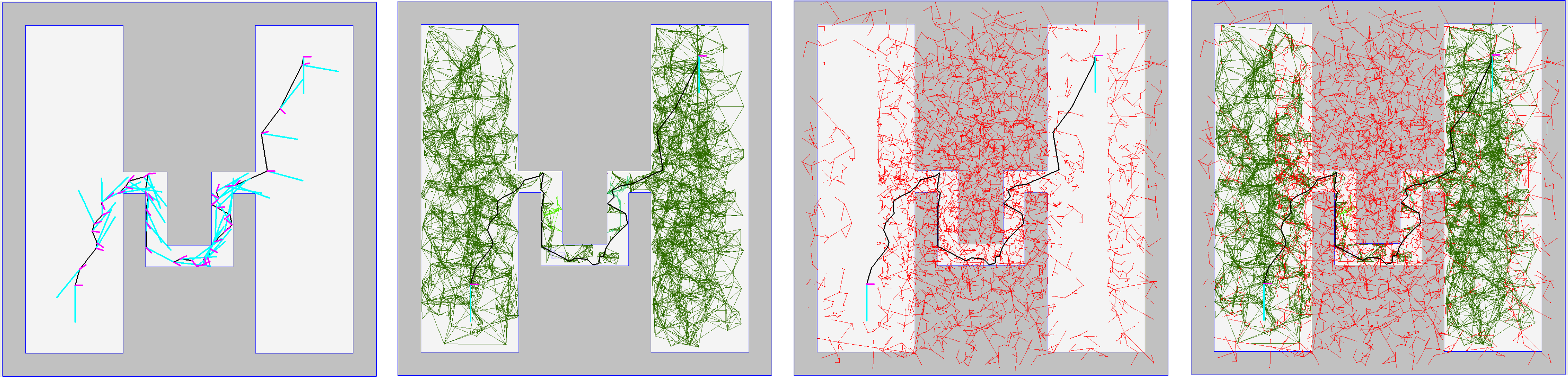
Figure 9: One Example Result of Toggle PRM: subfigures from left to right are its trace, free graph, obstacle graph, and mixed graph result.

Table 3 are experiments in Narrow Passages. While, Table 4 are in Easy Passages. For our SSS planner, $\varepsilon$ is equal to 1 for Table 3 and $\varepsilon$ is equal to 2 for Table 4. In these Tables, we time out a planner in $30$ seconds. In Table 3, most sampling planners reach the time limitation. On the other hand, SSS planner always produces a path or no-path within $4$ seconds. The worst average time of SSS is $3.646$ seconds when solving double bug trap environment with non-crossing 2-link robots. The best average time of SSS is $0.312$ seconds when solving 100 random triangles environment with crossing 2-link robots.

Table 3: Narrow Passages Result with Crossing and Non-crossing 2-link Robots

In Table 4, we decrease thickness $\tau$ to make it easier for Toggle PRM and Lazy Toggle PRM to find a path. In some situations, Toggle PRM and Lazy Toggle PRM may find the path almost as quickly as SSS. For example, in their best cases for the T-Room and 8-Way Corridor scenarios, Toggle PRM is about $1.6$ and $1.4$ times slower than SSS and Lazy Toggle PRM is approximately as fast as SSS. But, on average, SSS outperforms Toggle PRM and Lazy Toggle PRM by at least an order of magnitude. In conclusion, based on Tables 3 and 4, our SSS planners is superior to Toggle PRM and Lazy Toggle PRM with crossing and non-crossing 2-link robots.

Table 4: Easy Passages Result with Crossing and Non-crossing 2-link Robots

We have conducted an exhaustive experiment using $30$ minutes timeout for Tables 3 and 4. These results are recorded in Tables 3^* and 4^*. However, we only do a single run of each environment. By comparing it with our SSS planner and previous Toggle PRM results, giving more time does improve the success rates. For example, in the Narrow Passages scenario (Table 3^*), by taking more time, Toggle PRM can find a path in the T-Room, 100 Random Triangles, and Double Bug Trap environment in a single run with crossing 2-link robots. From Table 4^*, not only in the T-Room, 8 Way Corridors, Hole-in-Wall, and Double Bug Trap environment with crossing 2-link robots but also in the T-Room, 100 Random Triangles, and 8 Way Corridors with non-crossing 2-link robots, it can make obvious improvement. In another point of view, if sampling methods like Toggle PRM are likely to find a path, there is a trade-off between timeout limitation and success rates. On the other hand, in our SSS planner, there is no such trade-off.

Table 3^*: Narrow Passages Result with Crossing and Non-crossing 2-link Robots

Table 4^*: Easy Passages Result with Crossing and Non-crossing 2-link Robots

References

- [1] M. Barbehenn and S. Hutchinson. Toward an exact incremental geometric robot motion planner. In Proc. Intelligent Robots and Systems 95., volume 3, pages 39–44, 1995. 1995 IEEE/RSJ Intl. Conf., 5–9, Aug 1995. Pittsburgh, PA, USA.
- [2] R. A. Brooks and T. Lozano-Perez. A subdivision algorithm in configuration space for findpath with rotation. In Proc. 8th Intl. Joint Conf. on Artificial intelligence - Volume 2, pages 799–806, San Francisco, CA, USA, 1983. Morgan Kaufmann Publishers Inc.
- [3] H. Choset, K. M. Lynch, S. Hutchinson, G. Kantor, W. Burgard, L. E. Kavraki, and S. Thrun. Principles of Robot Motion: Theory, Algorithms, and Implementations. MIT Press, Boston, 2005.
- [4] J. Denny and N. M. Amato. Toggle PRM: A coordinated mapping of C-free and C-obstacle in arbitrary dimension. In WAFR 2012, volume 86 of Springer Tracts in Advanced Robotics, pages 297–312, 2012. MIT, Cambridge, USA. June 2012.
- [5] J. Denny, K. Shi, and N. M. Amato. Lazy Toggle PRM: a Single Query approach to motion planning. In Proc. IEEE Int. Conf. Robot. Autom. (ICRA), pages 2407–2414, 2013. Karlsrube, Germany. May 2013.
- [6] S. L. Devadoss and J. O’Rourke. Discrete and Computatational Geometry. Princeton University Press, 2011.
- [7] L. Kavraki, P. Švestka, C. Latombe, and M. Overmars. Probabilistic roadmaps for path planning in high-dimensional configuration spaces. IEEE Trans. Robotics and Automation, 12(4):566–580, 1996.
- [8] J. J. Kuffner Jr and S. M. LaValle. RRT-connect: An efficient approach to single-query path planning. In Robotics and Automation (ICRA 2000). IEEE International Conference on, volume 2, pages 995–1001. IEEE, 2000.
- [9] S. M. LaValle. Planning Algorithms. Cambridge University Press, Cambridge, 2006.
- [10] Z. Luo. Resolution-exact Planner for a 2-link planar robot using Soft Predicates. Master thesis, New York University, Courant Institute, Jan. 2014. Department’s Master Thesis Prize 2014.
- [11] Z. Luo, Y.-J. Chiang, J.-M. Lien, and C. Yap. Resolution exact algorithms for link robots. In Proc. 11th Intl. Workshop on Algorithmic Foundations of Robotics (WAFR ’14), volume 107 of Springer Tracts in Advanced Robotics (STAR), pages 353–370, 2015. 3-5 Aug 2014, Boǧazici University, Istanbul, Turkey.
- [12] J. Pan, L. Zhang, and D. Manocha. Retraction-based rrt planner for articulated models. In Proc. IEEE ICRA, pages 2529–2536, 2010.
- [13] O. Salzman, K. Solovey, and D. Halperin. Motion planning for multi-link robots by implicit configuration-space tiling, 2015. CoRR abs/1504.06631.
- [14] M. Sharir, C. O’D’únlaing, and C. Yap. Generalized Voronoi diagrams for moving a ladder II: efficient computation of the diagram. Algorithmica, 2:27–59, 1987. Also: NYU-Courant Institute, Robotics Lab., No. 33, Oct 1984.
- [15] I. Şucan, M. Moll, and L. Kavraki. The Open Motion Planning Library. IEEE Robotics & Automation Magazine, 19(4):72–82, 2012. http://ompl.kavrakilab.org.
- [16] C. Wang, Y.-J. Chiang, and C. Yap. On Soft Predicates in Subdivision Motion Planning. In 29th ACM Symp. on Comp. Geom., pages 349–358, 2013. SoCG’13, Rio de Janeiro, Brazil, June 17-20, 2013. Journal version in Special Issue of CGTA.
- [17] C. Yap, Z. Luo, and C.-H. Hsu. Resolution-exact planner for thick non-crossing 2-link robots. ArXiv e-prints, 2017. Submitted. See also proceedings of 12th WAFR, 2016, and http://cs.nyu.edu/exact/ for proofs and detail of experimental data.
- [18] C. K. Yap. Soft Subdivision Search in Motion Planning. In A. Aladren et al., editor, Proceedings, 1st Workshop on Robotics Challenge and Vision (RCV 2013), 2013. A Computing Community Consortium (CCC) Best Paper Award, Robotics Science and Systems Conference (RSS 2013), Berlin. In arXiv:1402.3213.
- [19] C. K. Yap. Soft Subdivision Search and Motion Planning, II: Axiomatics. In Frontiers in Algorithmics, volume 9130 of Lecture Notes in Comp.Sci., pages 7–22. Springer, 2015. Plenary Talk at 9th FAW. Guilin, China. Aug 3-5, 2015.
- [20] D. Zhu and J.-C. Latombe. New heuristic algorithms for efficient hierarchical path planning. IEEE Transactions on Robotics and Automation, 7:9–20, 1991.