GASP I: Gas stripping phenomena in galaxies with MUSE

Abstract

GASP (GAs Stripping Phenomena in galaxies with MUSE) is a new integral-field spectroscopic survey with MUSE at the VLT aiming at studying gas removal processes in galaxies. We present an overview of the survey and show a first example of a galaxy undergoing strong gas stripping. GASP is obtaining deep MUSE data for 114 galaxies at z=0.04-0.07 with stellar masses in the range $10^{9.2}$-$10^{11.5}M_{\odot}$ in different environments (galaxy clusters and groups, over more than four orders of magnitude in halo mass). GASP targets galaxies with optical signatures of unilateral debris or tails reminiscent of gas stripping processes (“jellyfish galaxies”), as well as a control sample of disk galaxies with no morphological anomalies. GASP is the only existing Integral Field Unit (IFU) survey covering both the main galaxy body and the outskirts and surroundings, where the IFU data can reveal the presence and the origin of the outer gas. To demonstrate GASP’s ability to probe the physics of gas and stars, we show the complete analysis of a textbook case of a “jellyfish” galaxy, JO206. This is a massive galaxy ($9\times 10^{10}M_{\odot}$) in a low-mass cluster ($\sigma\sim 500\rm\,km\,s^{-1}$), at a small projected clustercentric radius and a high relative velocity, with $\geq$90kpc-long tentacles of ionized gas stripped away by ram pressure. We present the spatially resolved kinematics and physical properties of gas and stars, and depict the evolutionary history of this galaxy.

=20

1 Introduction

How gas flows in and out of galaxies is one of the central questions in galaxy formation and evolution. In the current hierarchical paradigm, the hot gas in dark matter haloes cools, feeding the interstellar medium present in the galaxy disk and replenishing the cold gas stock that is needed to form new stars (White & Rees 1978, Efstathiou & Silk 1983). Any process that prevents the gas from cooling efficiently, or removes gas either from the halo or from the disk, has fundamental consequences for the subsequent galaxy history.

Gas-averse processes abound. Virial shock heating of circumgalactic gas is an obvious contender. According to hydro-cosmological simulations, above a critical halo mass of $\sim 10^{12}M_{\odot}$, the radiative cooling rate is not sufficient to prevent a stable virial shock, while cold gas streams can substain the gas inflow onto massive haloes only at $z>1-2$ (Birnboim & Dekel 2003, Kereš et al. 2005, Dekel & Birnboim 2006, Dekel et al. 2009). Thus, haloes with $M>10^{12}M_{\odot}$ at $z<1$ should be naturally deprived of their gas supply by virial shocks.

Circumgalactic gas might be prevented from cooling also by simply removing the hot gas halo in the so-called “strangulation” scenario (Larson et al. 1980, Balogh et al. 2000). Since the halo gas is more loosely bound to the galaxy than the disk gas, it can be more easily stripped either by ram pressure stripping or by tidal effects once a galaxy is accreted onto a more massive halo.

Both processes mentioned above leave intact the gas that is already in the disk. Several other mechanisms can instead affect the disk gas in a direct way. Their origin can be internal to galaxies themselves, such as galactic winds due to star formation or an active galactic nucleus (Veilleux et al. 2005, King & Pounds 2015, Erb 2015), or external (Boselli & Gavazzi 2006). Among the latter, there is ram pressure stripping due to the pressure exerted by the intergalactic medium (Gunn & Gott 1972), thermal evaporation (Cowie & Songaila 1977) and turbulent/viscous stripping (Nulsen 1982). All of these affect the gas, but not directly the stellar component of galaxies. Tidal mechanisms instead affect both gas and stars, and include strong galaxy interactions and mergers (Barnes & Hernquist 1992), tidal effects of a cluster as a whole (Byrd & Valtonen 1990) and the so-called “harassment”, that is the cumulative effect of several weak and fast tidal encounters (Moore et al. 1996).

While the cosmic web of gaseous filaments expected to feed galaxies can be observed (e.g. Cantalupo et al. 2012, 2014), pure-gas accretion onto galaxies is very difficult to probe observationally, and direct observational evidence is still rare (e.g. Sancisi et al. 2008, Bouché et al. 2013), except in specific cases like X-ray cooling flows (Peterson & Fabian, 2006).

Direct observations of gas flowing out of galaxies are relatively easier, though a complete picture of how and why galaxies lose gas is still far from being reached. Many studies lack the multiwavelength data required to know the fate of the different gas phases (molecular gas, neutral and ionized hydrogen, and X-ray gas), but detailed observations are beginning to accumulate for a few galaxies (e.g. Sun et al. 2010, Vollmer et al. 2012, Yagi et al. 2013, Jáchym et al. 2013, Abramson et al. 2011, 2016).

The survey presented in this paper focuses on those processes that affect the gas in the disk, and not the stellar component. The most convincing body of evidence for gas-only removal comes from observations of internally-driven outflows and ram pressure stripping.

Quasar-driven and starburst-driven massive outflows of the cold phase and the ionized phase are now observed both at low- and high-z, though what fraction of the outflowing gas rains back onto the galaxy is still an open question (Feruglio et al. 2010, Steidel et al. 2010, Fabian 2012, Bolatto et al. 2013, Genzel et al. 2014, Cicone et al. 2014, Wagg et al. 2014, Cresci et al. 2015).

HI studies have convincingly shown the efficiency of ram pressure stripping of the neutral gas in nearby galaxy clusters (e.g. Haynes et al. 1984, Cayatte et al. 1990, Kenney et al. 2004, Chung et al. 2009, Vollmer et al. 2010, Jaffé et al. 2015), and sometimes also in groups (e.g. Rasmussen et al. 2006, 2008, Verdes-Montenegro et al. 2001, Hess et al. 2013). Conclusions from molecular studies are more debated, but overall the molecular gas seems to be removed in clusters, though less efficiently than the atomic gas (cf. Kenney & Young 1989 and Boselli et al. 1997, Boselli et al. 2014). Ionized gas studies based on $\rm H\alpha$ imaging are another excellent tracer of gas stripping in clusters (e.g. Gavazzi et al. 2002, Yagi et al. 2010, Yoshida et al. 2012, Fossati et al. 2012, Boselli et al. 2016). Even more powerful are IFU studies, that are able to reveal the gas that is stripped and ionized and also provide the kinematical and physical properties of the ionized gas as well as the stars (Merluzzi et al. 2013, 2016, Fumagalli et al. 2014, Fossati et al. 2016). Hydrodynamical simulations of ram pressure stripping describe the formation of these gas tails and their evolution (Abadi et al. 1999, Quilis et al. 2000, Roediger & Brüggen 2007, Kapferer et al. 2008, Tonnesen & Bryan 2012, Tonnesen & Stone 2014, Roediger et al. 2014, see reviews by Roediger 2009 and Vollmer 2013).

Notably, stars are often formed in the stripped gas (e.g. Kenney & Koopmann 1999, Yoshida et al. 2008, Smith et al. 2010, Hester et al. 2010, Kenney et al. 2014, Jáchym et al. 2014). Galaxies in which stars are born within the stripped gas tails can therefore be identified also from ultraviolet or blue images, in which the newly born stars produce a recognizable signature (Cortese et al. 2007, Smith et al. 2010, Owers et al. 2012). The most striking examples of this are the so-called “jellyfish galaxies”, that exhibit tentacles of material that appear to be stripped from the galaxy body, making the galaxy resemble animal jellyfishes (Fumagalli et al. 2014, Ebeling et al. 2014, Rawle et al. 2014). In the last years, the first optical systematic searches for gas stripping candidates have been conducted (Poggianti et al. 2016, McPartland et al. 2016).

GASP is a new integral-field spectroscopy survey with MUSE aiming at studying gas removal processes from galaxies. It is observing 114 disk galaxies at z=0.04-0.07 comprising both a sample with optical signatures of unilateral debris/disturbed morphology, suggestive of gas-only removal processes, and a control sample lacking such signatures. Galaxies with obvious tidal features/mergers were purposely excluded. GASP is thus tailored for investigating those processes that can remove gas, and only gas, from the disk, though we cannot exclude that tidal effects are partly or fully responsible for the morphologies observed in some of the targets. The GASP data themselves will clarify the physical causes of the gas displacement. Being based on optical spectroscopy, this study can reveal the ionized gas component. Neutral and molecular studies of the GASP sample are ongoing, as described in §8.

The most salient characteristics of GASP are the following:

1) Galaxy areal coverage. In addition to the galaxy main body, the IFU data cover the galaxy outskirts, surroundings and eventual tails, out to $\sim 50-100$ kpc away from the main galaxy component, corresponding to $>10R_{e}$. The galaxy outskirts and surroundings are crucial for detecting the extraplanar gas and eventual stars. The combination of large field-of-view (1’$\times$1’) and sensitivity of MUSE at the GASP redshifts allows us to observe galaxies out to large radii, while maintaining a good spatial resolution ($\sim 1$ kpc). This is a unique feature of GASP, as other large IFU surveys typically reach out to $2.5-3R_{e}$ at most (see Table 3 in Bundy et al. 2015).

2) Environment. One of the main goals of GASP is to study gas removal processes as a function of environment, and understand in what environmental conditions are such processes efficient. GASP explores a wide range of environments, from galaxy clusters to groups and poor groups. Its targets are located in dark matter haloes with masses spanning four orders of magnitude ($10^{11}-10^{15}M_{\odot}$).

3) Galaxy mass range. GASP galaxies have a broad range of stellar masses ($10^{9.2}-10^{11.5}$), therefore it is possible to study the efficiency of gas removal processes and their effects on the star formation activity as a function of galaxy mass and size.

In this first paper of the series we present the GASP scientific goals (§2), describe the survey (§3), the observations (§4) and the analysis techniques (§6) and we show the results for a strongly ram-pressure-stripped massive galaxy in a low-mass cluster (§7). The current status and data release policy are described in §5. For the first results of the GASP survey, readers are refereed also to other papers of the first set (Bellhouse et al. Paper II, Fritz et al. Paper III, Moretti et al. Paper IV and Gullieuszik et al. Paper V).

In all papers of this series we adopt a standard concordance cosmology with $H_{0}=70\,\rm km\,s^{-1}\,Mpc^{-1}$, ${\Omega}_{M}=0.3$ and ${\Omega}_{\Lambda}=0.7$ and a Chabrier (2003) IMF.

2 Scientific drivers

The key science questions to be addressed with GASP are the following:

1. Where, why and how is gas removed from galaxies? (§2.1)

2. What are the effects of gas removal on the star formation activity and on galaxy quenching? (§2.2)

3. What is the interplay between the gas physical conditions and the activity of the galaxy central black hole? (§2.3)

4. What is the stellar and metallicity history of galaxies prior to and in absence of gas removal? (§2.4)

2.1 The physics of gas removal

GASP seeks the physical mechanism responsible for the gas removal. For each GASP galaxy, we address the following questions: Is gas being removed? By which physical process (ram pressure stripping, tidal effects, AGN etc)? What is the amount and fraction of gas that is being removed? GASP will evaluate this comparing the morphology and kinematics of the stellar and gaseous components of each galaxy using the stellar continuum and the emission lines in the MUSE spectra, respectively, and measuring gas masses from $\rm H\alpha$ fluxes as described in §6.3.

Whatever the gas removal process at work, the GASP data can shed light on the rich physics involved, observing how the gas removal proceeds and what are the timescales involved, how the kinematics and morphology of the gas are affected, whether there are large scale outflows, what are the metallicities and the dust content of the gas, and which is the cause for gas ionization (star formation, shocks, AGN). Most of these quantities can be directly measured from the MUSE spectra, either from individual lines (gas kinematics and morphology, outflows, see §6.2) or from the emission line ratios (metallicity, dust, ionization mechanism, see §6.3).

The general questions we wish to investigate with the complete GASP sample want to shed light on fundamental issues regarding the loss of gas from galaxies, such as: For which fraction of galaxies are gas-only removal processes relevant? For which types/masses of galaxies? In which environments? Only in clusters, or also in groups? Where in clusters (for which clustercentric distances/velocities/orbits etc)? And, is the efficiency of gas removal enhanced during halo-halo merging?

Ram pressure stripping calculations are obtained both with analytical methods and hydrodynamical simulations (e.g. Gunn & Gott 1972, Jaffe’ et al. 2015, and references above). They predict how the efficiency of gas stripping depends on the galaxy and environmental parameters under certain assumptions, which can be tested with the GASP sample. Moreover, there is some observational evidence that the efficiency of gas stripping is enhanced by shocks and strong gradients in the X-ray ICM (Owers et al. 2012, Vijayaraghavan & Ricker 2013), but only a large sample such as GASP can inequivocally determine a correlation and the necessary physical conditions. Finally, the first cosmological hydrodynamical simulations including the effects of ram pressure, tidal stripping and satellite-satellite encounters on the HI gas in different environments make predictions on the relative roles of the various mechanisms as a function of halo mass and redshift (e.g. Marasco et al. 2016). Studies like GASP are the natural observational counterparts to corroborate or reject the theoretical predictions.

2.2 Gas, star formation and quenching

Overall, the star formation activity in galaxies has strongly declined since $z\sim 2$, for the combination of two effects: a large number of previously star-forming galaxies have evolved into passive (i.e. has stopped forming stars), and the star formation rate in still star-forming galaxies has, on average, decreased (Guglielmo et al. 2015). Innumerable observational evidences point to this, including the evolution of the passive fraction with time and the evolution of the star formation rate–stellar mass relation (e.g. Bell et al. 2004, Noeske et al. 2007). On a cosmic scale, this leads to a drop in the star formation rate density of the Universe (Madau & Dickinson 2014).

One of the most debated questions is what drives the star formation decline. The availability of gas is central for this problem. The simplest explanation is that galaxies “run out of gas”: they are deprived of gas repenishment due to virial shocks or strangulation, and consume the disk gas for star formation. In alternative, or in addition, they can have their star formation shut off by one or more of the internal or external physical processes acting on the disk gas, described in the previous section.

GASP provides the spatially resolved ongoing star formation activity and star formation history. Thus, the GASP data allow us to link the gas removal process with its effects on the galaxy stellar history, determine whether the star formation activity is globally enhanced, or suppressed due to the mechanism at work, and how the quenching of star formation proceeds within the galaxy and on what timescale. The goal is to understand how many stars are formed in the stripped gas, how the extraplanar star formation contributes to the intergalactic medium and, more in general, what is the impact of gas-only removal processes for galaxy quenching.

2.3 Gas and AGN

While supermassive black holes are thought to be ubiquituous at least in massive galaxies, an Active Galactic Nucleus (AGN) powered by accretion of matter onto the black hole is much rarer (Kormendy & Ho 2013, Brinchmann et al. 2004). Several candidates have been proposed as “feeding mechanisms” able to trigger the AGN activity. These include all those processes that can cause large scale gas inflow in the galaxy central regions, such as gravitational torques due to galaxy mergers or interactions (Di Matteo et al. 2005, Hopkins et al. 2006), or disk instability due for example to high turbulent gas surface densities maintained by cold streams at high-z (Bournaud et al. 2011).

The availability of gas, or lack thereof, is thus an essential ingredient for feeding the black hole, and mechanisms affecting the gas are also believed to influence the AGN (e.g. Sabater, Best & Heckman 2015). Given that the gas content of galaxies is especially sensitive to environmental effects, AGN studies as a function of enviroment are of interest, though they often find contrasting results (Miller et al. 2003, Kauffmann et al. 2004, Martini et al. 2006, Popesso & Biviano 2006, von der Linden et al. 2010, Marziani et al. 2016).

GASP can investigate the link between the gas availability, gas physical conditions, and AGN activity. The IFU data permit an investigation of the galaxy central regions of all galaxies, a detailed analysis of the gas ionization source (thanks to the large number of emission lines included in the spectra) and the detection of eventual AGN-driven large-scale outflows. Future GASP papers will present the occurrence of AGN among ram-pressure stripped galaxies (e.g. Poggianti et al. 2017b submitted). As an example, the galaxy presented in this paper hosts an AGN (§7.2).

2.4 Galaxy evolution without and before stripping

The GASP control sample consists of disk galaxies with a range of galaxy masses and in different environments, with no sign of disturbance/debris. At all effects, they can be considered a sample of “normal galaxies”. Moreover, the GASP stripping candidates undergoing gas-only removal processes have their stellar component undisturbed, retaining the memory of the galaxy history before stripping. Thus, from the stellar component of the MUSE datacube with our spectrophotometric code we can recover the past galaxy history at times before the stripping occurred (see §6.2).

Thus, GASP can be used to derive the spatially resolved stellar and metallicity history in absence, or prior to, galaxy removal, as well as the ongoing star formation activity and ionized gas properties in normal galaxies.

Compared to other larger IFU surveys (Sánchez et al. 2012, Allen et al. 2015, Bundy et al. 2015), GASP has the disadvantage of the smaller number of galaxies, but the advantage of covering many galactic effective radii. The outer regions of galaxies hold a unique set of clues about the way in which galaxies are assembled (Ferguson et al. 2016). With GASP it is possible to peer into galaxy outskirts, to study the stellar, gas and dust content out to large radii in galaxies, enabling to compare the star formation history and metallicity gradients with simulations of disk galaxy formation (Mayer et al. 2008, Vogelsberger et al. 2014, Kauffmann et al. 2016, Christensen et al. 2016). GASP observations are suitable to investigate how star formation occurs at low gas densities and low metallicities, and may hold clues about stellar migration and satellite accretion.

3 Survey strategy

3.1 Parent surveys: WINGS, OMEGAWINGS and PM2GC

The GASP program is based on three surveys that, together, cover the whole range of environmental conditions at low redshift: WINGS, OMEGAWINGS and PM2GC.

WINGS is a multiwavelength survey of 76 clusters of galaxies at z=0.04-0.07 in both the north and the south emisphere (Fasano et al. 2006). The clusters were selected on the basis of their X-ray luminosity (Ebeling et al. 1996, 1998, 2000) and cover a wide range in halo mass ($10^{13.6}-10^{15.2}\,M_{\odot}$), with velocity dispersions $\sigma=$ 500-1300 $\rm km\,s^{-1}$ and X-ray luminosities $\rm L_{X}=10^{43.3-45}\,\rm erg\,s^{-1}$. The original WINGS dataset comprises deep B and V photometry with a $34^{\prime}\times 34^{\prime}$ field-of-view with the WFC@INT and the WFC@2.2mMPG/ESO (Varela et al. 2009), spectroscopic follow-ups with 2dF@AAT and WYFFOS@WHT (Cava et al. 2009), J and K imaging with WFC@UKIRT (Valentinuzzi et al. 2009) and U-band imaging (Omizzolo et al. 2014). The WINGS database is presented in Moretti et al. (2014) and is all publicly available through the Virtual Observatory.

OMEGAWINGS is a recent extension of the WINGS project that has quadrupled the area covered in each cluster (1 square degree). B and V deep imaging with OmegaCAM@VST was secured for 46 WINGS clusters (Gullieuszik et al. 2015), a $u$-band program is ongoing with the same instrument (D’Onofrio et al. in prep.) and an AAOmega@AAT spectroscopic campaign yielded 18.000 new redshifts (Moretti et al. 2017) together with stellar population properties and star formation rates that have been used in Paccagnella et al. (2016).

As a comparison field sample we use the Padova Millennium Galaxy and Group Catalogue (PM2GC, Calvi et al. 2011), which is drawn from the Millennium Galaxy Catalogue (MGC, Liske et al. 2003). The MGC data consist of deep B-band imaging with WFC@INT over a 38 $deg^{2}$ equatorial area and a highly complete spectroscopic follow-up (96% at B=20, Driver et al. 2005). The PM2GC galaxy sample is thus representative of the general field and as such contains galaxy groups (176 with at least three members at z=0.04-0.1), binary systems and single galaxies, as identified with a Friends-of-friends algorithm by Calvi et al. (2011), covering a braod range in halo masses (Paccagnella et al. in prep.).

3.2 Selection of GASP targets

GASP is planning to observe 114 galaxies, of which 94 are primary targets and 20 compose a control sample.

3.2.1 Primary targets: the Poggianti et al. (2016) atlas

GASP primary targets were taken from the atlas of Poggianti et al. (2016, hereafter P16), who provided a large sample of galaxies whose optical morphologies are suggestive of gas-only removal mechanisms. These authors visually inspected B-band WINGS, OMEGAWINGS and PM2GC images searching for galaxies with (a) debris trails, tails or surrounding debris located on one side of the galaxy, (b) asymmetric/disturbed morphologies suggestive of unilateral external forces or (c) a distribution of star-forming regions and knots suggestive of triggered star formation on one side of the galaxy. Galaxies whose morphological disturbance was clearly induced by mergers or tidal interactions were deliberately excluded. The selection was based only on the images, therefore a subset of the candidates did not have a known spectroscopic redshift. For the PM2GC, only galaxies with a spectroscopic redshift in the range of WINGS clusters (z=0.04-0.07) were considered.

P16 classified candidates according to the strength of the optical stripping signatures: JClass 5 and 4 are those with the strongest evidence and are the most secure candidates, including classical “jellyfish galaxies” with tentacles of stripped material; JClass 3 are probable cases of stripping, and JClass 2 and 1 are the weakest, tentative candidates.

After inspecting a total area of about 53 $deg^{2}$ in clusters (WINGS+OMEGSAWINGS) and 38 $deg^{2}$ in the field (PM2GC), the total P16 sample consists of 344 stripping candidates in clusters (WINGS+OMEGAWINGS) and 75 candidates in the field (PM2GC), finding apparently convincing candidates for gas-only removal mechanisms also in groups down to low halo masses. While for cluster galaxies the principal culprit is commonly assumed to be ram pressure stripping, this is believed to be too inefficient in groups and low-mass haloes, where other mechanisms, such as undetected minor or major mergers or tidal interactions, might give rise to similar optical features. The integral field spectroscopy obtained by GASP is the optimal method to identify the physical process at work, because it probes both gas and stars and can discriminate processes affecting only the gas, such as ram pressure, from those affecting gas and stars, such as tidal effects and mergers.

The P16 candidates are all disky galaxies with stellar masses in the range $\sim 10^{9}-10^{11.5}\,M_{\odot}$ and are mostly star-forming with a star formation rate that is enhanced on average by a factor of 2 compared to non-candidates of the same mass.

GASP will observe as primary targets 64 cluster and 30 field stripping candidates taken from the P16 atlas. They are selected according to the following criteria: (a) be observable from Paranal (DEC$<+15$); (b) include all the JClass=5 objects; (c) include galaxies of each JClass, from 5 to 1, in similar numbers; (d) for WINGS+OMEGAWINGS, give preference to spectroscopically confirmed cluster members, rejecting known non-members; (e) cover the widest possible galaxy mass range.

Spatially resolved studies of gas in cluster galaxies have shown that the stripping signatures visible in the optical images are just the tip of the iceberg: the stripping is much more evident from the ionized gas observations than in the optical (Merluzzi et al. 2013, Fumagalli et al. 2014, Kenney et al. 2015). For this reason we chose to include in our study galaxies with a wide range of degree of evidence for stripping (of all Jclasses plus a control sample), to obtain a complete view of gas removal phenomena.

Figure 1: Top. Galaxy stellar mass distributions of cluster (right, WINGS/OMEGAWINGS) and group/field targets (left, PM2GC) for the primary sample (solid black histogram) and the control sample (dashed green histograms). Bottom. Host halo mass distributions of WINGS/OMEGAWINGS (to the right of the dotted horizontal line) and PM2GC (to the left of the line) targets. All these distributions are subject to change (see text).

Figure 1 presents the galaxy stellar mass and host halo mass distributions of GASP primary and control targets, that are similar to those of their parent samples in Poggianti et al. (2016). At this stage these distributions are preliminary and incomplete, but already allow the reader to gauge the range of masses covered. They are preliminary because the final sample that will be observed may not be exactly the same we envisage at the moment, due to observability, scheduling etc. in service mode; they are incomplete because for now we have galaxy mass estimates only for the subset of targets with WINGS/OMEGAWINGS/PM2GC spectroscopy, while MUSE will provide masses for each galaxy. Final properties of the sample, together with the complete list of targets, will be published in subsequent paper of this series once the observations are finalized.

3.2.2 The control sample

Galaxies in the control sample are galaxies in clusters (12) and in the field (8) with no optical sign of stripping, i.e. no signs of debris or unilaterally disturbed morphologies in the optical images. This sample will allow to contrast the properties of stripping candidates with those of galaxies that show no optical evidence of gas removal. Finding signs of gas stripping from the IFU data even in galaxies of the control sample would reveal that the stripping phenomenon is more widespread than it is estimated from the optical images. Moreover, the control sample represents a valuable dataset of “normal” disk galaxies that allows a spatially resolved study out to several galaxy effective radii.

Control sample galaxies were selected from WINGS, OMEGAWINGS and PM2GC visually inspecting the same B-band images used for the primary targets and were chosen according to the following criteria: (a) be at DEC$<+15$ (b) for WINGS+OMEGAWINGS, be spectroscopically confirmed cluster members; (c) have a stellar mass estimate from the spectral fitting (Paccagnella et al. 2016 for WINGS+OMEGAWINGS, Calvi et al. 2011 for PM2GC) and cover a galaxy mass range as similar as possible to that of the primary targets (Fig. 1); (d) be spirals spanning the same morphological range of the primary targets (Sb to Sd), with the addition of a few lenticulars and early spirals for comparison. For both WINGS/OMEGAWINGS and PM2GC, the morphologies are derived with the MORPHOT automatic classification tool (Fasano et al. 2012, Calvi et al. 2012); (e) include both star-forming (emission-line), post-starburst (k+a/a+k) and passive (k) spectral types according to the definition in Fritz et al. (2014).

4 Observations and data reduction

Observations are currently undergoing and are carried out in service mode using the MUSE spectrograph located at the Nasmyth B focus of the Yepun (Unit Telescope 4) VLT in Paranal. The constraints demanded for the observations are: clear conditions, moon illumination $<30\%$, moon distance $>30$ degrees , and image quality $<0.9\rm\,arcsec$, corresponding to $<1\rm\,arcsec$ seeing at zenith.

MUSE (Bacon et al. 2010) is composed of 24 IFU modules, equipped with 24$\times$4k$\times$4k CCDs. We use the MUSE wide-field mode with natural seeing that covers approximately a 1’$\times$1’ field-of-view with 0.2”$\times$0.2” pixels. The spectral range between 4800 Å  and 9300 Å  is sampled with a resolution FWHM$\sim 2.6$ Å  (R=1770 at 4800 Å  and =3590 at 9300 Å ) and a sampling of 1.25 Å/pixel. Thus, each datacube yields approximately 90.000 spectra.

4.1 Observing strategy

The majority of GASP galaxies are observed with 4 exposures of 675 sec each, each rotated by 90 degree and slightly offsetted with respect to the previous one, to minimise the cosmetics. The minimum time on target is therefore 2700 sec per galaxy. Some targets, however, show long tails in the optical images and require two, or even three, offsetted pointings to cover the galaxy body and the lenght of the tails. Each of these pointings is covered with 2700 sec, split into 4 exposures, as above.

The great majority of pointings have a significant fraction of sky coverage, while for a few galaxies it is necessary to do a 120 sec sky offset after each 675 sec exposure, because the galaxy fills the MUSE FOV.

Standard calibration frames are taken for each observation according to the ESO MUSE Calibration Plan. In short, at least one spectrophotometric standard star was observed each night for flux and telluric correction purpose. An internal illumination correction flat is also taken near the beginning or the end of the observations to minimise flatfielding issues due to ambient temperature changes. Daytime calibrations such as arcs, biases, darks, and flats (both internal and sky) are also taken. Static calibrations such as astrometry, line-spread-functions etc come as default in the pipeline supplied by ESO.

4.2 Data reduction

The data are reduced with the most recent version of the MUSE pipeline at any time (Bacon et al. 2010, https://www.eso.org/sci/software/pipelines/muse/). This was version 1.2 for the first data taken, and is v.1.6 at the time of writing. The procedures and philosophy of the data-reduction follow closely those set out in the ESO Pipeline Manual. To speed up and automate the process, raw data are organised and prepared with custom scripts, then fed to ESOREX recipes v.3.12. For most observations, the pipeline can be run in a semi automated fashion, since the observations are mostly identical in the execution and calibration. Briefly, the pipeline is run with mainly default parameters. The data and the standard star frames are flat-fielded, wavelength calibrated and corrected for differential atmospheric refraction. Typical wavelength calibration has $\approx 0.025$ Å  RMS in the fit, and the mean resolution $R$ measured from the arcs is about 3000.

As explained above, most of the exposures have sufficient sky coverage within the MUSE field-of-view, leaving $>50\%$ area for sky measurements, and the sky is modeled directly from the individual frames using the $20\%$ pixels with the lowest counts, thus there is no risk of accidentally subtracting any faint diffuse H$\alpha$ within the FOV. For spatially extended galaxies the offset sky exposures of 120s allow the sky to be modelled adequately.

The standard star observation closest in time to the science observations is used for the flux calibration. After flux calibration and telluric correction, the final flux-calibrated datacube is generated by lining up the individual frames using sources in the white-light images to calculate the (small) offsets. Galaxies with multiple pointings use sources in the overlaps for alignment. In a few cases we found no sources in the overlap: we therefore computed the offsets using custom scripts and OMEGAWINGS images as reference.

MUSE spectra in the red, where strong skylines dominate, are known to have residuals of sky subtraction in the current pipeline implementation. As the most interesting absorption and emission lines for our galaxies lie blueward of 7200 Å, this issue does not pose a problem. When the red part of the spectrum is needed for analysis, we perform a further cleaning of the spectrum redward of 7200 Å  using ZAP (Soto et al 2016) which provides satisfactory results. However experimentation of ZAP shows that it has to be used with caution, especially if there may be faint extended $\rm H\alpha$ emission in the “sky” spaxels which ZAP can aggressively “clean”.

5 Current status and data products release policy

At the time of writing, in January 2017, 55 out of the 114 targets have been observed. All data taken have been reduced. Based on the current rate of execution, we project a completion by the end of 2018.

GASP is an ESO Large Program committed to release its products into the ESO Science Archive. These products will include input target catalogs, fully reduced and calibrated MUSE datacubes, catalogs with redshifts and emission-line fluxes for galaxy spaxels and catalogs of outputs of our spectrophotometric model SINOPSIS (Fritz et al. submitted, Paper III) with stellar masses, stellar ages and star formation histories.

6 Data analysis

This section describes the procedure we use to analyze all galaxies of the survey. The chart in Fig. 2 presents the work-flow described below. In the following, we first describe the spectral analysis spaxel by spaxel, then we consider the integrated spectra of individual star-forming knots (§6.4) and of the galaxy main body (§6.5). Extraplanar knots of star formation turn out to be common in GASP galaxies and therefore are an important aspect of our analysis.

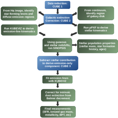
Figure 2: Schematic chart of the GASP analysis work-flow (see text for details).

First of all, the reduced datacube is corrected for extinction due to our own Galaxy, using the extinction value estimated at the galaxy position (Schlafly & Finkbeiner 2011) and assuming the extinction law from Cardelli et al. (1989). The corrected datacube (CUBE 2 in Fig. 2) is used in all the subsequent analysis.

6.1 Gas and stellar kinematics

To analyze the main emission lines in the spectrum we use the IDL publicly available software KUBEVIZ (Fossati et al. 2016), written by Matteo Fossati and David Wilman. Starting from an initial redshift, KUBEVIZ uses the MPFit (Markwardt 2009) package to fit gaussian line profiles, yielding gaseous velocities (with respect to given redshift), velocity dispersions and total line fluxes. The list of emission lines fitted by KUBEVIZ is given in Table 1, together with the characteristic surface brightness $3\sigma$ limit for each line.

Table 1: Emission lines fitted with KUBEVIZ for this study.

Line	$\lambda$	$\mu_{lim}$
	(Å) (air)	$\rm erg\,s^{-1}\,cm^{-2}\,arcsec^{-2}$
$\rm H\beta$	4861.33	0.3 – 1.6 $\times 10^{-17}$
$\rm[OIII]$	4958.91	0.3 – 1.2 $\times 10^{-17}$
$\rm[OIII]$	5006.84	0.3 – 1.2 $\times 10^{-17}$
$\rm[OI]$	6300.30	0.2 – 0.8 $\times 10^{-17}$
$\rm[OI]$	6363.78	0.3 – 0.9 $\times 10^{-17}$
$\rm[NII]$	6548.05	0.2 – 1.0 $\times 10^{-17}$
$\rm H\alpha$	6562.82	0.2 – 1.1 $\times 10^{-17}$
$\rm[NII]$	6583.45	0.2 – 1.0 $\times 10^{-17}$
$\rm[SII]$	6716.44	0.2 – 0.8 $\times 10^{-17}$
$\rm[SII]$	6730.81	0.2 – 0.8 $\times 10^{-17}$

KUBEVIZ uses “linesets”, defined as groups of lines that are fitted simultaneously. Each lineset (e.g. $\rm H\alpha$ and [NII]6548, 6583) is considered a combination of 1D Gaussian functions keeping the velocity separation of the lines fixed according to the line wavelengths. KUBEVIZ imposes a prior on the velocity and instrinsic line width of each lineset, which is fixed to that obtained by the fit of the $\rm H\alpha$ and [NII] lines. Moreover, the flux ratios of the two [NII] and [OIII] lines are kept constant in the fit assuming the ratios given in Storey & Zeippen (2000).

Before carrying out the fits, the datacube is average filtered in the spatial direction with a 5$\times$5 pixel kernel, corresponding to 1 arcsec=0.7-1.3 kpc depending on the galaxy redshift. Moreover, as recommended by Fossati et al. (2016), the errors on the line fluxes are scaled to achieve a reduced ${\chi}^{2}=1$. KUBEVIZ can attempt a single or a double component fit. A single fit was run for each galaxy, while another KUBEVIZ run with a double component was necessary in some cases, as described in Paper II. The continuum is calculated between 80 and 200 Å  redwards and bluewards of each line, omitting regions with other emission lines and using only values between the 40th and 60th percentiles.

Maps of $\rm H\alpha$ intensity, velocity and velocity dispersion are created at this stage using the KUBEVIZ output. The original datacube is visually and carefully inspected, and contrasted with these maps, for a) finding fore- and back-ground sources that are superimposed on the galaxy of interest along the line of sight. A mask of these sources is created in order to remove the contaminated regions from the stellar analysis described below and, b) checking the output of KUBEVIZ and ensuring all lines are correctly identified.

To extract the stellar kinematics from the spectrum, we use the Penalized Pixel-Fitting (pPXF) code (Cappellari & Emsellem, 2004), fitting the observed spectra with the stellar population templates by Vazdekis et al. (2010). We used SSP of 6 different metallicities (from $[M/H]=-1.71$ to $[M/H]=0.22$) and 26 ages (from 1 to 17.78 Gyr) calculated with the Girardi et al. (2000) isochrones. Given the poor resolution of the theoretical stellar libraries in the red part of the spectra, and the strong contamination from the sky lines in the observed spectra redwards of the $\rm H\alpha$ region, we run the code on the spectra cut at $\sim 7000$ Å  restframe. We first accurately masked spurious sources (stars, background galaxies) in the galaxy proximity, that could enter one of the derived bins. After having degraded the spectral library resolution to our MUSE resolution, we first find spaxels belonging to the galaxy, here defined as those with a signal median-averaged over all wavelengths larger than $3\times 10^{-20}\,\rm ergs^{-1}cm^{-2}{\AA}^{-1}$ per spaxel. Then we performed the fit of spatially binned spectra based on signal-to-noise (S/N=10, for most galaxies), as described in Cappellari & Copin (2003), with the Weighted Voronoi Tessellation modification proposed by Diehl & Statler (2006). This approach allows to perform a better tessellation in case of non Poissonian noise, not optimally weighted pixels and when the Centroidal algorithm introduces significant gradients in the S/N.

We derived maps of the rotational velocity, the velocity dispersion and the two h3 and h4 moments using an additive Legendre polynomial fit of the 12th order to correct the template continuum shape during the fit. This allows us to derive for each Voronoi bin a redshift estimate, that was then used as input for the stellar population analysis.

6.2 Emission line fluxes and stellar properties

To obtain the measurements of total emission line fluxes, corrected for underlying stellar absorption, and for deriving spatially resolved stellar population properties we run our spectrophotometric model SINOPSIS (Paper III). This code searches the combination of single stellar population (SSPs) spectra that best fits the equivalent widths of the main lines in absorption and in emission and the continuum at various wavelengths, minimizing the ${\chi}^{2}=1$ using an Adaptive Simulated Annealing algorithm (Fritz et al. 2011, 2007). The star formation history is let free with no analytic priors.

The code, which has been employed to derive star formation histories and rates, stellar masses and other stellar properties of various surveys (Dressler et al. 2009, Fritz et al. 2011, Vulcani et al. 2015, Guglielmo et al. 2015, Paccagnella et al. 2016, Cheung et al. 2016) has been substantially updated and modified for the purposes of GASP. The GASP version of SINOPSIS is fully described in Paper III, here we only describe the main improvements with respect to Fritz et al. (2011). The code now uses the latest SSPs model from Charlot & Bruzual (in prep.) with a higher spectral and age resolution. They use a Chabrier (2003) IMF with stellar masses in the 0.1–-100 M_⊙ limits, and they cover metallicity values from $Z=0.0001$ to $Z=0.04$. These models use the latest evolutionary tracks from Bressan et al. (2012) and stellar atmosphere emission from a compilation of different authors, depending on the wavelength range, and on the stellar luminosity and effective temperature. In addition, nebular emission has been added for the youngest (i.e.age $<2\times 10^{7}$ years) SSP, by ingesting the original models into CLOUDY (Ferland et al. 2013). In this way, the SSP spectra we use display also the most common and most intense emission lines (e.g. Hydrogen, Oxygen, Nitrogen). Moreover, the code has been improved and optimised to deal efficiently with datacubes such as the products from MUSE. It is now possible to read in the observed spectra directly from the cube fits file, while the redshifts for each spaxel are taken from 2D redshift masks.

SINOPSIS requires the spectrum redshift as input, thus the redshift at each location of the datacube was taken from pPXF (stellar) and KUBEVIZ (gaseous) as described above. As the stellar and gas components might be kinematically decoupled, the observed wavelength of a given line in emission (gas) could differ from that of the same line in absorption (stellar photosphere). This might result in an erroneous measurement of the line, depending on which redshift is adopted, introducing issues most of all for the H$\beta$ line, where the emission and absorption components can be separately identified. Hence, we have introduced a further option in SINOPSIS to allow the use of the gas redshift, when available, to detect and measure the equivalent width of emission lines, while the stellar redshift is used to fit the continuum and measure absorption lines. The code is then run on the 5$\times$5 pixel average filtered observed cube.

SINOPSIS produces a best fit model cube (stellar plus gaseous emission) and a stellar-only model cube (containing only the stellar component). The latter is subtracted from the observed datacube to provide an emission-only cube (CUBE 3 in Fig. 1) that is used for all the following analysis. KUBEVIZ is run a second time ($\rm KUBEVIZ_{run2}$) on this emission-only cube to estimate the emission line fluxes corrected for stellar absorption.

In addition, SINOPSIS gives spatially resolved estimates of the stellar population properties, and maps are produced for: a) stellar masses; b) average star formation rate and total mass formed in 4 age bins: young(ongoing SF)=$<2\times 10^{7}$ yr; recent=$2\times 10^{7}<5.7\times 10^{8}$ yr; intermediate age= $5.7\times 10^{8}<5.7\times 10^{9}$ yr; old=$>5.7\times 10^{9}$ yr; c) luminosity-weighted stellar ages.

6.3 Derived quantities: dust extinction, gas metallicity, diagnostic diagrams, star formation rates and gas masses

The emission-line, absorption-corrected fluxes measured by $\rm KUBEVIZ_{run2}$ are then corrected for extinction by dust internal to the galaxy. The correction is derived from the Balmer decrement at each spatial element location assuming an intrinsic $\rm H\alpha$/$\rm H\beta$ ratio equal to 2.86 and adopting the Cardelli et al. (1989) extinction law. This yields dust- and absorption-corrected emission line fluxes and a map of the dust extinction $A_{V}$. These fluxes are then used to derive all the quantities discussed below.

The gas metallicity and $q$ ionization parameter are calculated at each spatial location using the pyqz code (Dopita et al. 2013) v0.8.2. The $q$ parameter is defined by Dopita et al. (2013) as the ratio between the number of ionizing photons per unit area per second and the gas particle number density . The code interpolates a finite set of diagnostic line ratio grids computed with the MAPPINGS code to compute $\log(Q)$ and $12+\log(O/H)$. The MAPPINGS V grids in pyqz v0.8.2 cover a limited range in abundances ($8.11\leq 12+log(O/H)\leq 8.985$); we therefore used a modified version of the code to implement MAPPINGS IV grid tested in the range $7.39\leq 12+log(O/H)\leq 9.39$ (F. Vogt, priv. communication). We used the calibration based on the strong emission lines, namely [NII]6583/[SII]6716,6731 vs [OIII]5007/[SII]6716,6731 . Using only one diagnostic could in principle lead to systematic effects both on the ionization parameter and on the metallicity values, as shown in Dopita et al. (2013). However, conclusions based on differential analyses of metallicity variations/gradients within a galaxy are not affected by this problem.

The line fluxes are also used to create line-ratio diagnostic diagrams (Baldwin et al. 1981, BPT) to investigate the cause of the gas ionization and distinguish regions photoionized by hot stars from regions ionized by shocks, LINERs and AGN. Only spaxels with a S/N$>3$ in all the emission lines involved are considered. For each galaxy we inspect and compare the conclusions based on three diagrams: [OIII]5007/$\rm H\beta$ vs [NII]6583/$\rm H\alpha$, [OIII]5007/$\rm H\beta$ vs [OI]6300/$\rm H\alpha$ and [OIII]5007/$\rm H\beta$ vs [SII]6717,6731/$\rm H\alpha$.

The SFR of each spatial element is computed from the $\rm H\alpha$ luminosity corrected for dust and stellar absorption adopting Kennicutt (1998)’s relation:

$$SFR=4.6\times 10^{-42}L_{H\alpha}$$ (1)

where SFR is in solar masses per year and the $\rm H\alpha$ luminosity is in erg per second, for a Chabrier IMF.

The total SFR is computed from the sum of the dust-corrected $\rm H\alpha$ fluxes in each spaxel, after removing hot pixels and adopting a S/N cut (between 3 and 7). The same method is used to compute the SFR within the “galaxy body” (i.e. the stellar outer isophotes described in sec. 6.5). The latter can also be computed with SINOPSIS from the integrated spectrum, but only without removing the AGN contribution.

The $\rm H\alpha$ luminosity can be employed to estimate the mass of ionized gas (e.g. Boselli et al. 2016). From Osterbrock & Ferland (2006, eqn. 13.7, pag. 344):

$$L_{H\alpha}=n_{e}n_{p}Vf\alpha_{H\alpha}h\nu_{H\alpha}$$ (2)

where V is the volume, f the filling factor, $n_{e}$ and $n_{p}$ are the density of electrons and protons, $\rm\alpha_{H\alpha}$ is the effective $\rm H\alpha$ recombination coefficient ($1.17\times 10^{-13}cm^{3}\,s^{-1}$) and $\rm h\nu_{H\alpha}$ is the energy of the $\rm H\alpha$ photon ($0.3028\times 10^{-11}erg$) for a case B recombination, n=10000 $\rm cm^{-3}$, and T=10000 K. It is commonly assumed that $n_{e}$=$n_{p}$=$n$ (the gas is fully ionized, e.g. Boselli et al. 2016, Fossati et al. 2016).

The mass of ionized gas is the number of hydrogen atoms (=number of protons) times the mass of the hydrogen atom $m_{H}=1.6735\times 10^{-24}gr$. The number of protons is equal to the density of protons times the volume times the filling factor $N_{protons}=n_{p}Vf$. Using eqn.(2) above we compute the ionized gas mass as:

$$M_{gas}=N_{protons}\times m_{p}=\frac{L_{H\alpha}\times m_{p}}{n\alpha_{H\alpha}h\nu_{H\alpha}}$$ (3)

The density $n$ can be derived from the ratio of the [SII]6716 and [SII]6732 lines. We use the calibration from Proxauf et al. (2014) for T=10000 K, obtained with modern atomic data using CLOUDY, which is valid for the interval $R=[SII]6716/[SII]6732=0.4-1.435$.

6.4 Star-forming knots

The majority of GASP galaxies present bright star-forming knots in the gaseous tails and/or in the galaxy disk.

The location and radius of these knots are found through a purposely devised shell script that includes IRAF and FORTRAN calls. In the first step, the centers of knot candidates are identified as local minima onto the laplace+median filtered $\rm H\alpha$ image derived from the MUSE datacube (IRAF-laplace and IRAF-median tools). A ”robustness index” is then associated to each local minimum, based on the gradient concordance towards the knot center for pixels around the minimum. The final catalog of knot positions includes the local minima whose ”robustness index” exceeds a given value. In the second step the knot radii are estimated from the original $\rm H\alpha$ image and their photometry is performed by a purposely devised FORTRAN code. In particular, the blob’s radii are estimated through a recursive (outwards) analysis of three at a time, consecutive circular shells (thickness: 1 pixel) around each knot center. The iteration stops and the knot’s radius is recorded when at least one among the following circumstances occurs for the current outermost shell: (a) the counts of at least one pixel exceed those of the central pixel; (b) the fraction of pixels with counts greater than the average counts of the preceding shell (’bad’ pixels) exceeds a given maximum value (usually 1/3); (c) the average counts of ‘good’ (not ’bad’) pixels is lower than a given threshold value, previously set for the diffuse emission; (d) the image edges are reached by at least one pixel.

The knot radii provided in this way are used to obtain, for each knot, the following photometric quantities: (1) total counts inside the circle defining the knot, both including and excluding the counts below the threshold previously set for the diffuse emission (counts of pixels belonging to different knots are equally shared among them); (2) total counts from integration of the growth curve. The average shell counts tracing the growth curve are obtained using only the ‘good’ pixels in each shell and the growth curve is extrapolated down to the diffuse emission threshold.

Besides the centers and the above mentioned measures for each knot, the final catalog associated to each $\rm H\alpha$ image provides a number of useful global photometric quantities of the $\rm H\alpha$ image, including: (a) total counts coming from the knots according to the three measures described above; (b) total counts attributable to the diffuse emission, both including and excluding the pixels inside the knot’s circles; (c) total counts of pixels with counts above the diffuse emission threshold, but laying outside the knot’s circles.

KUBEVIZ (run3) is then run on a mask identifying all the knots, producing emission line fits for the integrated, emission-only spectrum of each knot. The line fluxes are corrected for dust extinction and used to derive for each knot diagnostic diagrams, gas metallicity estimates, star formation rate measurements and ionized gas mass estimates with the methods described in sec. 6.3.

6.5 Integrated galaxy spectrum

Finally, we integrate the spectrum over the galaxy main body to obtain a sort of “total galaxy body spectrum”. To this aim, KUBEVIZ is used to obtain a 2D image of the near-$\rm H\alpha$ continuum. The spaxels belonging to the galaxy main body are identified slicing this image at two different count levels, with a surface brightness difference of $\sim$2-2.5 mag. The outer isophote encloses essentially all the galaxy body, down to $\sim 1\sigma$ above the background level. Since the signal-to-noise ratio is not the same for all galaxies, this implies that the corresponding surface brightness is different for different galaxies. The inner isophote contains the bright part of the galaxy, usually 70-75% of the total counts within the outer isophote. It is worth noting that, due to the different morphological features of galaxies, the inner cut has been visually chosen, varying interactively the colormap of the galaxy image. This means that also the surface brightness of the inner isophote is not the same for all galaxies.

SINOPSIS is run on the galaxy integrated spectrum obtained within each of the two isophotal contours to derive the global stellar population properties.

7 A textbook-case jellyfish galaxy: JO206

The quality and characteristics of GASP data, which is very homogeneous for all targets, is best illustrated showing the results for one galaxy of the sample, JO206 (z=0.0513, WINGS J211347.41+022834.9), which was selected as a JClass=5 stripping candidate in the poor cluster IIZW108 (z=0.0486, Moretti et al. 2017). JO206 is present in both the OMEGAWINGS (Gullieuszik et al. 2015) and WINGS (Varela et al. 2009) images, at RA=21 13 47.4 DEC= +02 28 35.5 (J2000). An RGB (u, B and V bands) image of the central region of this cluster is shown in Fig. 3, with JO206 and the Brightest Cluster Galaxy (BCG) highlighted. No spectroscopic redshift was available before it was observed by GASP.

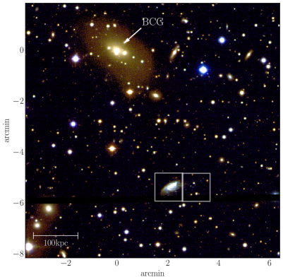
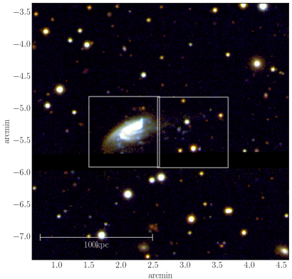
Figure 3: Left. RGB image (OMEGAWINGS u, WINGS B and V) of the central region of the cluster IIZW108, with the forming BCG and the two MUSE pointings for JO206 highlighted. North is up, and east is left. Right. The same RGB image zoomed on JO206.

JO206 was observed with two MUSE pointings ($2700$ sec each) on August 7 2016, with 1” seeing during the first pointing and 1.2 arcsec during the second pointing. From the GASP integrated disk galaxy spectrum, defined as described in §6.5, SINOPSIS yields a total galaxy stellar mass 8.5$\times 10^{10}M_{\odot}$ within the outer isophote, a total ongoing SFR=$\sim 7M_{\odot}\,yr^{-1}$, and a luminosity weighted age of $\sim 1$Gyr.

The MUSE white image (Fig. 4, 4750-9350 Å) displays faint traces of tails with knots to the west of the galaxy body: they are the reason why this galaxy was selected as stripping candidate in the first place. The extent of the stripped gas becomes much more striking in the MUSE $\rm H\alpha$ map (Fig. 5, left). $\rm H\alpha$ emission is observed in the galaxy disk, in a projected 40kpc-wide extraplanar region to the south-west of the disk and in tentacles extending 90kpc to the west, giving this galaxy the classical jellyfish shape. Additional MUSE pointings would be needed to investigate how far beyond the edge of the image the tails extend. Both in the galaxy disk and in the stripped gas, the $\rm H\alpha$ image is characterized by regions of diffuse emission and brighter emission knots, which will be studied individually in §7.4. Moreover, in the NW region of the disk, the enhancement of $\rm H\alpha$ emission could be related to gas compression due to the ram pressure stripping, as in Merluzzi et al. (2013).

The $\rm H\alpha$ signal-to-noise ratio (SNR) map is shown in Fig. 5 (right) for all spaxels with $S/N>4$. The data reach a surface brightness detection limit of $V\sim 27\rm mag\,arcsec^{-2}$ and $log\rm H\alpha\sim-17.6\,erg\,s^{-1}\,cm^{-2}\,arcsec^{-2}$ at the $3\sigma$ confidence level.

7.1 Gas and stellar kinematics

The $\rm H\alpha$ velocity map (Fig. 6, left) shows that the gas is rotating as the stars (Fig. 7, left), and that also the stripped gas maintains a coherent rotation for almost 60kpc downstream. This is similar to what is observed in ESO137-001, a jellyfish galaxy in the Norma cluster, in which the stripped gas retains the imprint of the disk rotational velocity 20kpc downstream along a 30kpc tail of ionized gas (Fumagalli et al. 2014). This signature indicates the galaxy is moving fast in the plane of the sky.

The velocity structure of the tentacles reveals that the longest tail (darkest tail between 10 and 60 arcsec in the left top panel of Fig. 6) is separated in velocity from the other tails and is probably trailing behind at higher negative speed than the rest of the gas (thus the galaxy velocity vector points away from the observer), likely having been stripped earlier than the other gas. This corresponds to a region of higher velocity dispersion ($\sigma$) of the gas (Fig. 6, right), which might indicate either that turbulent motion is setting in, or that there is gas at slightly different velocities along the line of sight. Inspecting the spectra, it is hard to distinguish between these two possibilities given the faintness of the emission in this region. Another region of high $\sigma$ is found at the southern edge of the gas south of the disk: a visual inspection of the spectra show that here we are probably seeing the superposition along the line of sight of gas at different location and velocities: a foreground higher velocity, and a background lower velocity component likely stripped sooner.

Most of the other gaseous regions and knots outside of the disk have very low $\sigma$ (0-20/50 $\rm km\,s^{-1}$), indicative of a dynamically cold medium. The high velocity dispersion at the center, instead, is due to the presence of an AGN, that will be discussed more in detail below.

In contrast with the complicated velocity structure of the gas, the stellar component has very regular kinematics showing that the disk is rotating unperturbed (Fig. 7, left), with a rather low velocity dispersion (mostly between 40 and 80 $\rm km\,s^{-1}$, Fig. 7, right), as it is typical of galaxy disks. The ordered stellar rotation, together with the regular isophotes, demonstrates that the process responsible for the gas stripping is affecting only the galaxy gas, and not the stars, as expected for ram pressure stripping due to the ICM.

The difference between the stellar and gaseous velocities would suggest a different direction of motion of the galaxy than the one suggested by the extended tail (cf. Fig. 8 and Fig. 6). However, simulations indicate that the stripped gas in the vicinity of the galaxy might not always be a reliable indicator of the direction of motion (Roediger & Brüggen 2006). The long tails indicate that the galaxy also has a significant velocity component in the tangential direction, on the plane of the sky.

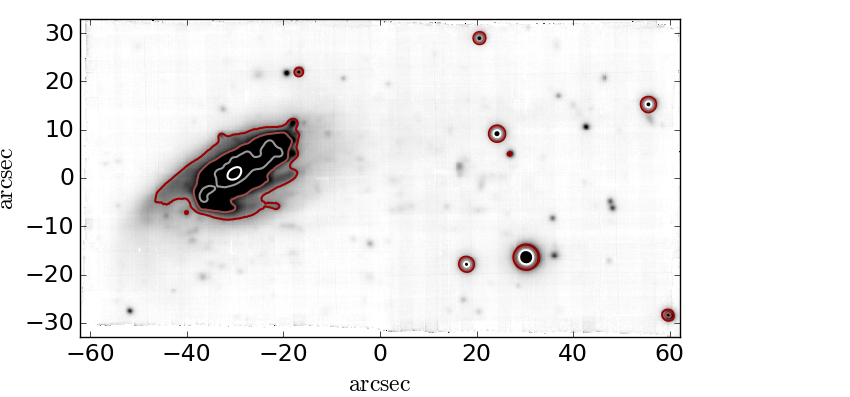
Figure 4: MUSE white image of JO206. Contours are logarithmically spaced isophotes of the continuum underlying $\rm H\alpha$, thus are stellar isophotes, down to a surface brightness $2.5\times 10^{-18}\rm\,ergs^{-1}cm^{-2}{\AA}^{-1}arcsec^{-2}$. Round isolated contours are Galactic stars that are masked in the subsequent analysis. In this and all plots (0,0) is the center of the MUSE combined image. North is up and east is left.

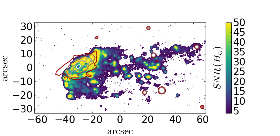
Figure 5: Left. MUSE $\rm H\alpha$ map (median filtered $5\times 5$ pixels) for $\rm H\alpha$ S/N$>4$, uncorrected for stellar absorption and intrinsic dust extinction, but corrected for Galactic extinction. The arrow indicates the direction to the BCG/X-ray center. At the cluster redshift, 1 arcsec = 0.952 kpc, see scale. Contours are continuum isophotes as in Fig. 4. Round isolated contours are Galactic stars. Right. $\rm H\alpha$ SNR map for median filtered $5\times 5$ pixels with S/N$>4$.

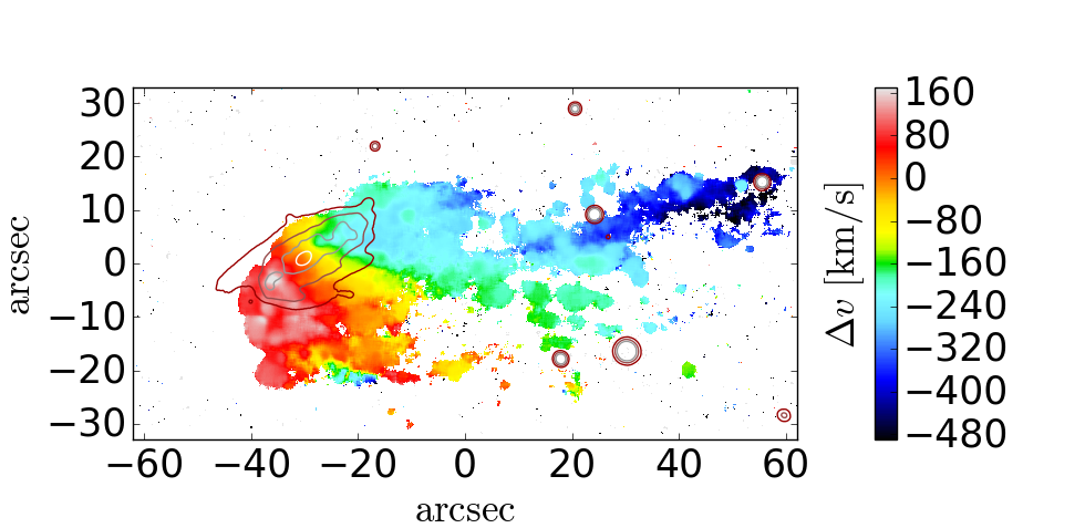
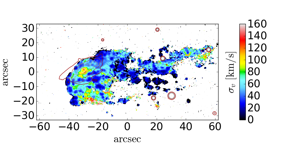
Figure 6: Top. $\rm H\alpha$ velocity (left) and velocity dispersion (right) map for $5\times 5$ spaxels with $S/N_{H\alpha}>4$. Contours are stellar isophotes, as in Fig. 4. $v=0$ corresponds to the redshift of the galaxy center (z=0.05133). Bottom. Corresponding error maps.

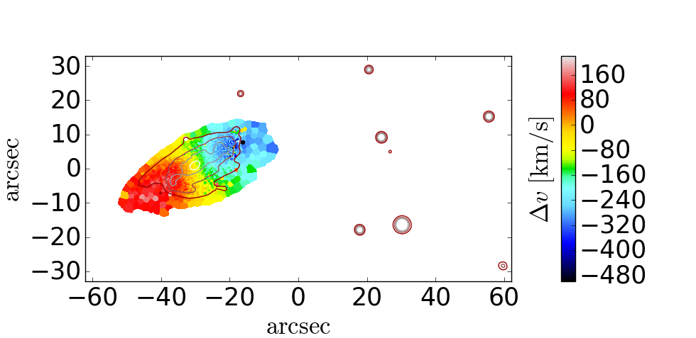
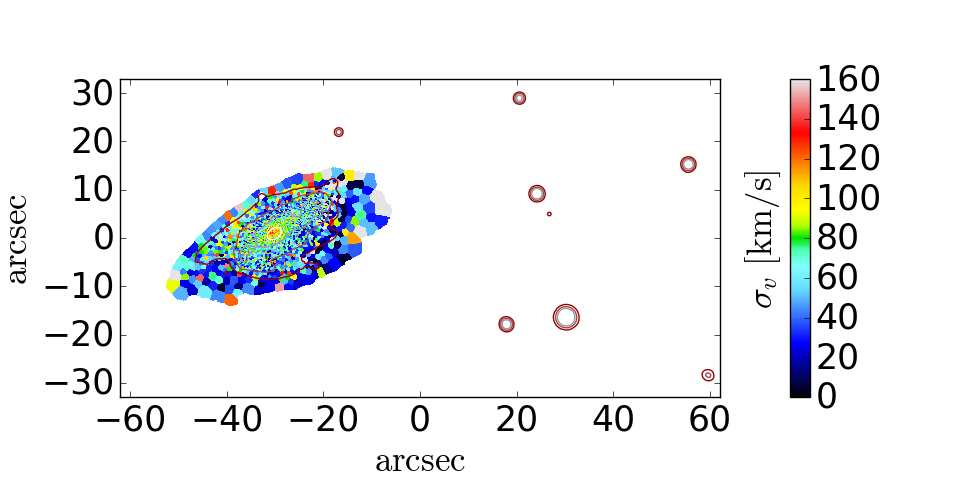
Figure 7: Stellar velocity (left) and velocity dispersion (right) map for Voronoi bins with S/N$>10$. Contours are stellar isophotes, as in Fig. 4.

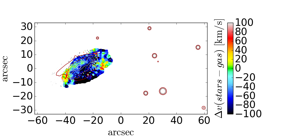
Figure 8: Velocity difference between stars and gas. Contours are stellar isophotes as in Fig. 4.

7.2 Gas ionization mechanism

The line ratio diagrams reveal that the emission in the central region is dominated by an AGN (Fig. 9). All three diagnostic diagrams inspected are concordant on this.

The presence of an AGN in this galaxy was previously unknown. A posteriori, we find that JO206 coincides within the position error with a ROSAT bright source (EXSS 2111.2+0217, Voges et al. 1999), hence we conclude it is an X-ray emitting AGN. The presence of an X-ray point source at the location of JO206 is also hinted by the map presented in Shang & Scharf (2009). Moreover, there is a 1.4 GHz NVSS detection within 8 arcsec from the position of JO206 (Condon et al. 1998). Using the calibration from Hopkins et al. (2003), the 1.4Ghz flux would yield a SFR of about 12 $M_{\odot}\,yr^{-1}$, which is a factor of 2 higher than the SFR measured from $\rm H\alpha$ (see §7.5). The properties of the AGN in JO206 and in other GASP jellyfish galaxies will be discussed in a separate paper (Poggianti et al. 2017b, submitted).

Apart from the center, the [OIII]5007/$\rm H\beta$ vs [NII]6583/$\rm H\alpha$ and vs [SII]6717,6731/$\rm H\alpha$ diagrams show that in the rest of the disk and in all the extraplanar gas (including the tentacles), the emission-line ratios are consistent with gas being photoionized by young stars (“Star-forming” according to Kauffmann et al. 2003 and Kewley et al. 2006) or a combination of Star-forming and HII-AGN Composite, the latter around the central region and in a stripe of intense H$\alpha$ brightness running almost north-south to the north-west of the galaxy. The [OIII]5007/$\rm H\beta$ vs [OI]6300/$\rm H\alpha$ diagram classifies the ionization source in these regions as LINERS, due to the significant [OI] emission, which supports the hypothesis that some contribution from shocks might be present here.

What stars are responsible for the majority of the ionizing radiation? We know that in order to produce a significant number of ionizing photons, they must be massive stars formed during the past $\leq 10^{7}$yr. They can either be new stars formed in situ, within the stripped gas, or stars formed in the galaxy disk whose ionizing radiation is able to escape to large distances. The first hypothesis is much more likely than the second one for several reasons: a) the tails and knots are faint but visible in the observed B-band light, which at the galaxy redshift should originate from stars with no significant contribution from line emission. In fact, the MUSE spectra at the location of $\rm H\alpha$ emission in the tentacles usually have a faint but detectable continuum; b) as we will show in §7.5, the MUSE spectra in the tails can be fitted with our spectrophotometric code with an amount of young stars that can account for the required ionizing photons and, at the same time, is consistent with the observed continuum level; c) if ionizing photons could travel for 90kpc without encountering any medium to ionize, the ionized gas we see would be the only gas there is in this area, and this is very unlikely.

Therefore, we conclude that, except for the central region powered by the AGN, the ionization source in JO206 is mostly photoionization by young stars. The most likely explanation is that new massive stars are born in situ in the stripped gas tentacles, and ionize the gas we observe. Our findings resemble the conclusions from Smith et al. (2010) regarding star formation taking place within the stripped gas in a sample of 13 jellyfish galaxies in the Coma cluster and support their hypothesis that this is a widespread phenomenon in clusters, though JO206 demonstrates that this does not occur only in rich, massive clusters such as Coma (see §7.6).

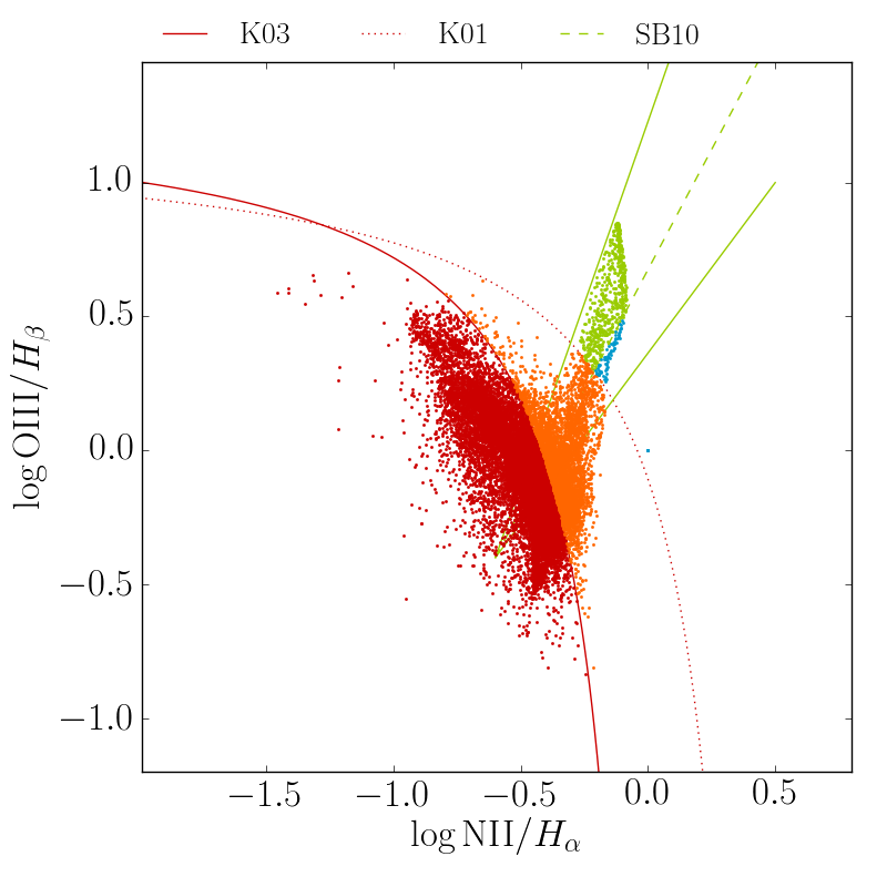
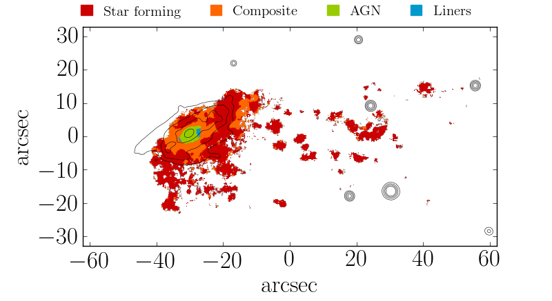
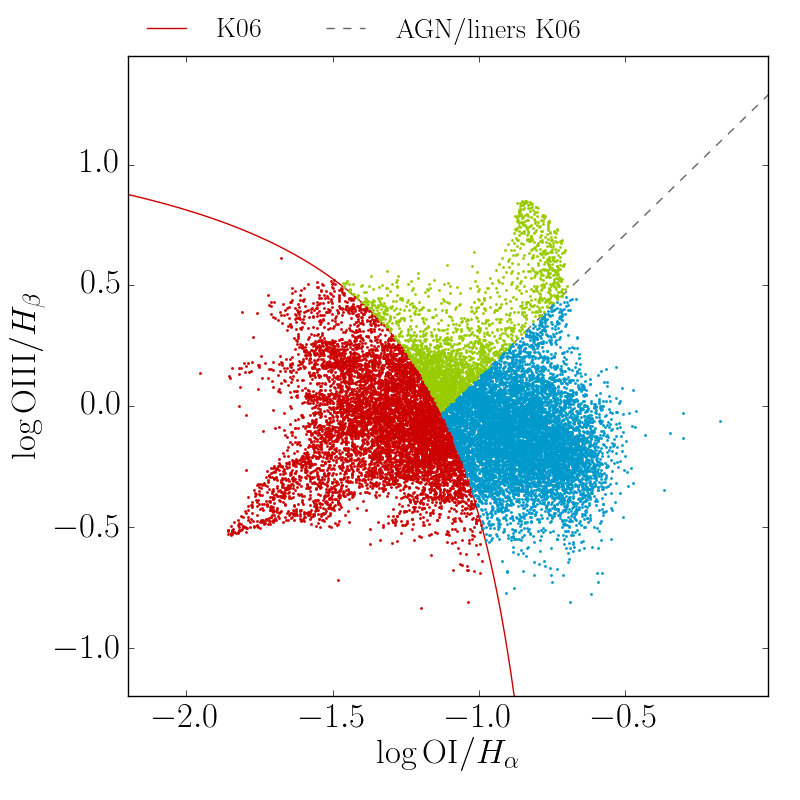
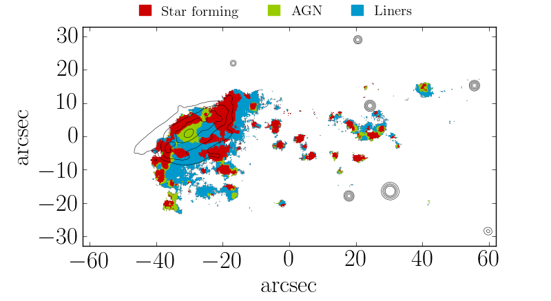
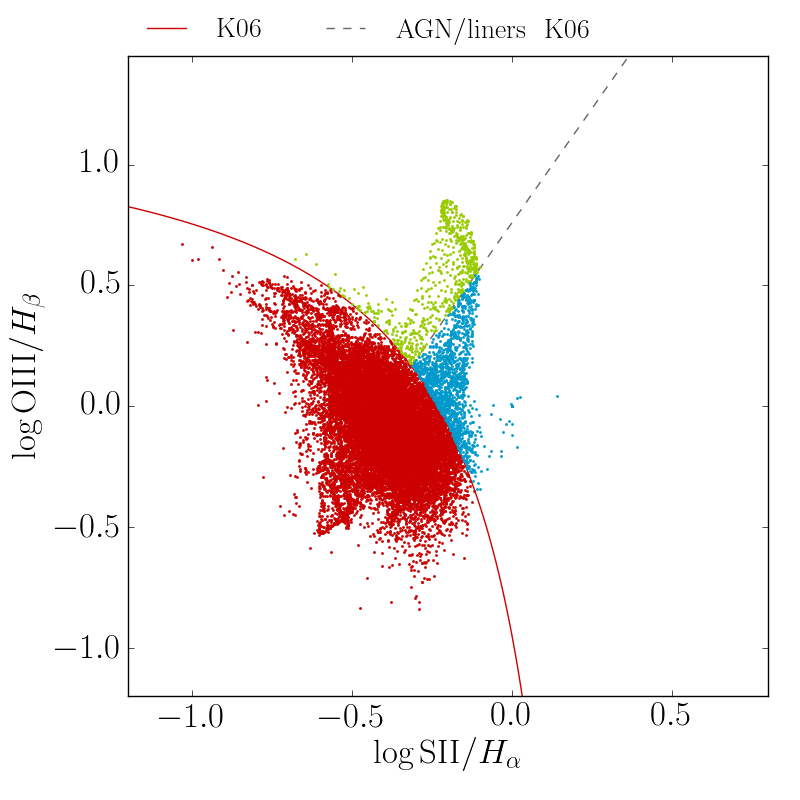
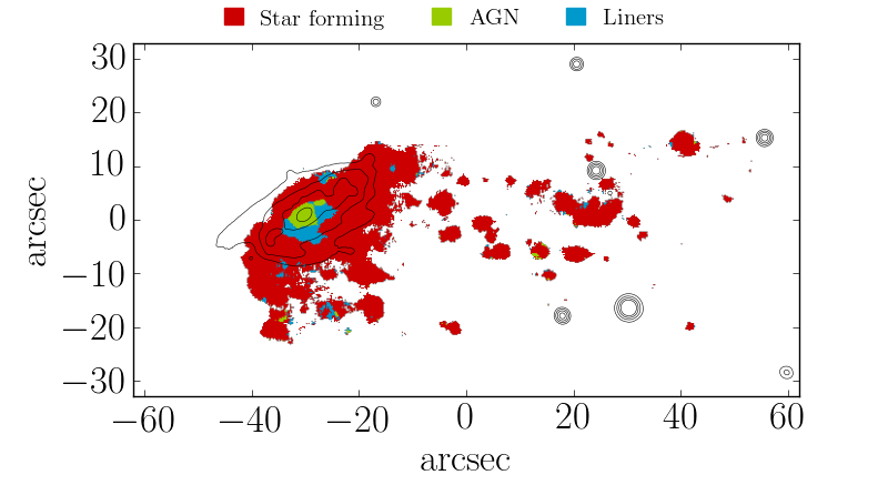
Figure 9: BPT line-ratio diagrams (left) and maps (right) for [OIII]5007/$\rm H\beta$ vs [NII]6583/$\rm H\alpha$ (top), vs [OI]6300/$\rm H\alpha$ (middle), and vs [SII]6717/$\rm H\alpha$ (bottom). Lines in the left panels are from Kauffmann et al. (2003, K03), Kewley et al. (2001, K01, and 2006, K06) and Sharp & Bland-Hawthorn (2010, SB10) to separate Star-forming, Composite, AGN and LINERS. Contours are stellar isophotes, as in Fig. 4.

7.3 Dust extinction and metallicity

The extinction map of Fig. 10 shows that the dust is not uniformly distributed, but concentrated in knots of rather high extinction (up to $A_{V}\sim 1.7$ mag), and inter-knots regions of lower extinction values (typically 0.5-0.6 mag), with edges of virtually no extinction. Knots of high extinction are found in the disk but also in the tentacles, far away from the galaxy disk. Interestingly, most of the high-extinction regions coincide with the knots of most intense H$\alpha$ emission that will be discussed in §7.4, identified in Fig. 10 by small circles. Thus, dust appears to be concentrated in the regions with higher H$\alpha$ brightness, hence higher SFR density, as it happens in HII regions in normal galaxies.

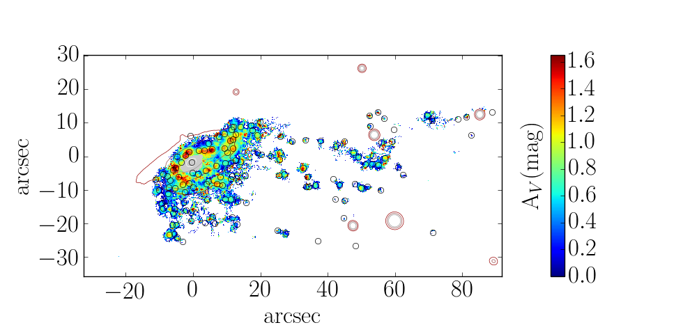
Figure 10: $A_{V}$ map. The small circles identify the location of the knots that are discussed in §7.4. The circle radius is fixed for all knots and is not proportional to the knot radius. The central region powered by the AGN according to the BPT [NII]6583/$\rm H\alpha$ diagnostic has been masked (grey area). Contours are stellar isophotes and round isolated contours are Galactic stars, as in Fig. 4.

The gas metallicity varies over almost 1dex in 12+log[O/H], with the highest metallicity regions located in the galaxy disk (Fig. 11, left). Interestingly, the most metal rich gas is observed $\sim 10$kpc from the center, to the north-west of the disk. This is a star-forming region of particularly high $\rm H\alpha$ brightness (Fig. 5, left), where the SFR per unit area is very high, and with rather high dust extinction (Fig. 10).

The metallicity in the tentacles is intermediate to low, reaching values as low as 12+log[O/H]=7.7-8 in the furthest regions of the west tail and throughout the southern tail. Overall, the gas at the end of the tentacles, likely to be the first that was stripped (as testified by its projected distance from the galaxy body and/or its velocity/$\sigma$), has a lower metallicity. This is coherent with a scenario in which the gas in the outer regions of the disk, which is the most metal poor, is stripped first, being the least bound.

Finally, the right panel of Fig. 11 shows that the ionization parameter is very low (generally $log\,q<7$) compared to the distribution measured in SDSS emission-line galaxies of all masses (always $>7$, typically $7.3$, Dopita et al. 2006). As the ionization parameter depends on several quantities (metallicity, IMF, age of the HII region, ISM density distribution, geometry etc), attempting an interpretation for the low values observed will require an in-depth analysis which is beyond the scope of this paper, but will be carried out on the whole stripped+control GASP sample.

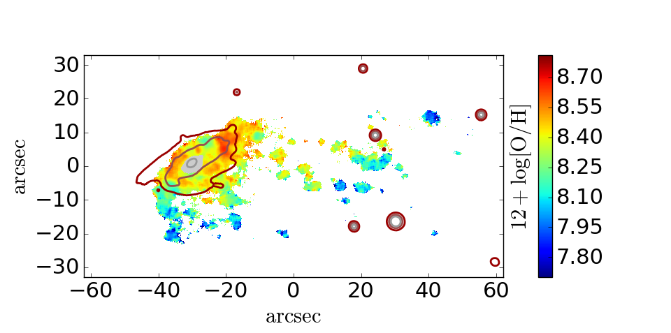
Figure 11: Metallicity (left) and ionization parameter (right) map. The central region powered by an AGN according to the BPT [NII]6583/$\rm H\alpha$ diagnostic has been masked (grey area). Contours are stellar isophotes as in Fig. 4.

7.4 Star-forming knots

We identify 139 individual knots in the JO206 H$\alpha$ image, as described in §6.4 and shown in Fig. 12. These are regions of high H$\alpha$ surface brightness, typically log ($\rm H\alpha[ergs^{-1}cm^{-2}arcsec^{-2}])\sim-15.5$. Figure 13 shows that, except for the central H$\alpha$ knot dominated by the AGN and a few small surrounding knots powered by a Composite source, the spectra of all the other knots are consistent with photoionization from young stars.

We note that MUSE revealed $\rm H\alpha$ knots also in the tails of ESO137-001 (Fossati et al. 2016) and these authors conclude these are HII regions formed in situ, as we find for JO206. In situ condensation of stripped gas is also found by Yagi et al. (2013) in the star-forming regions around NGC4388 in Virgo, and other extragalactic HII regions are known in Virgo (Cortese et al. 2004, Gerhard et al. 2002). In contrast, Boselli et al. (2016) conclude that NGC4569, a spectacular jellyfish in Virgo studied with narrow-band $\rm H\alpha$+[NII] imaging, lacks star-forming regions in the tail and therefore suggest that the gas is excited by mechanisms other than photoionization (e.g. shocks, heat conductions etc.). It will be interesting to understand how common are HII regions in jellyfish tails once the whole GASP sample is available, see for example the galaxies JO201 in Paper II and JO204 in Paper V.

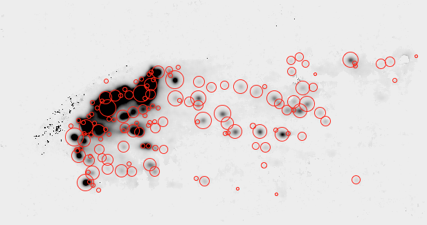
Figure 12: $\rm H\alpha$ flux map (black) with $\rm H\alpha$ knots as red circles.

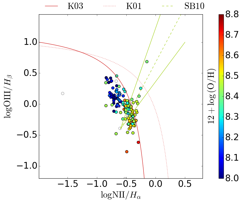
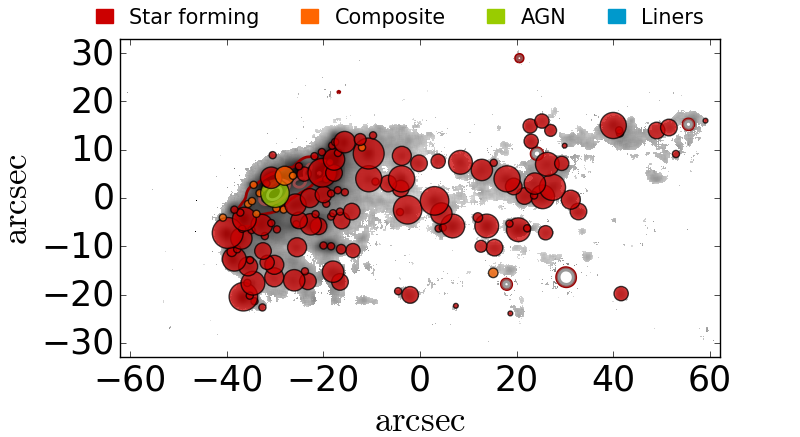
Figure 13: Left. BPT diagram of the $\rm H\alpha$ knots, color-coded by metallicity. Right. Spatial distribution of the knots, color-coded by ionization source. Here the radius of the circle corresponds to the radius of the knot (see sec. 6.4). The grey shaded area represents the $\rm H\alpha$ image.

In our MUSE data the metallicity of the gas in the knots varies with knot location (Fig. 14), and traces the spatially resolved metallicity shown in Fig. 11. The knots south of the disk, on the southern side of the main tail and those at the highest distances in the tail to the west are mostly metal poor (12+log(O/H)=8.0-8.2). The majority of the rest of the knots have intermediate metallicities (8.3-8.4), while the most metal rich significant knots are located along the disk north-west of the galaxy center.

Thus, the numerous knots we observe in JO206 appear to be giant HII regions and complexes. We estimate the ongoing SFR in each knot as described in §6.3. The sum of the SFR in all knots is 5.2 $M_{\odot}\,yr^{-1}$. The $\rm H\alpha$ luminosity of the only knot powered by the AGN corresponds to $\sim 1M_{\odot}\,yr^{-1}$, thus the total SFR in all blobs excluding the AGN is $\sim 4.2M_{\odot}\,yr^{-1}$. The SFR distribution of the knots is shown in Fig. 15. It ranges from a minimum of $\sim 10^{-4}$ to a maximum of 0.8 $M_{\odot}\,yr^{-1}$ per individual knot, and the average is about 0.01 $M_{\odot}\,yr^{-1}$. The SFR determination has several important caveats. These values are derived assuming a Chabrier IMF, but the true shape of the IMF in the knots is unconstrained. Even assuming a known IMF, at such low values of SFR of individual knots, the stochasticity of the IMF sampling can be important and will be the subject of a subsequent study.

The distributions of the ionized gas densities of the individual knots are shown in Fig. 15. Of the 138 knots with no AGN, 91 have a [SII]6716/[SII]6732 ratio in the range where the density calibration applies (see §6.3). The remaining knots have ratio values larger than 1.44, which suggests that their density is below 10 $\rm cm^{-3}$. Figure 15 shows that the most of the measured densities are between 10 and 100 $\rm cm^{-3}$, with a median of 28 $\rm cm^{-3}$. For these, we derive the ionized gas mass following eqn. 3 to derive the knot gas mass distribution also shown in Fig. 15. Most of these knots have masses in the range $10^{4}-10^{6.5}M_{\odot}$, with a median of $\sim 1.5\times 10^{5}M_{\odot}$. Summing up the gas mass in these knots we obtain $1.7\times 10^{8}\,M_{\sun}$, which represents a hard lower limit to the total ionized gas mass, given that the contributions of the knots with no density estimate and of the diffuse line emission are not taken into account. However, considering that the knots contributing to this mass estimate already account for about half of the total $L_{\rm H\alpha}$, the total mass value given above is probably of the order of the true value.

Once star formation will be exhausted in JO206 blobs, they will probably resemble the UV “fireballs” in the tail of IC3418, a dIrr galaxy in Virgo with a tail of young stellar blobs ($<$400 Myr, Fumagalli et al. 2011, Hester et al. 2010, Kenney et al. 2014).

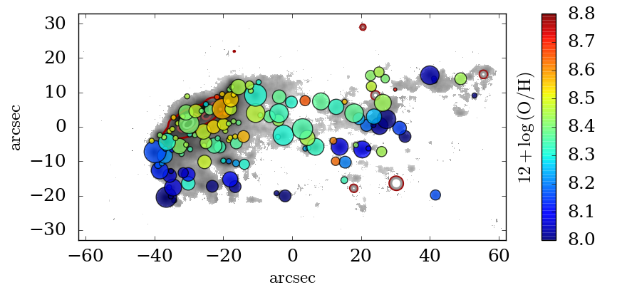
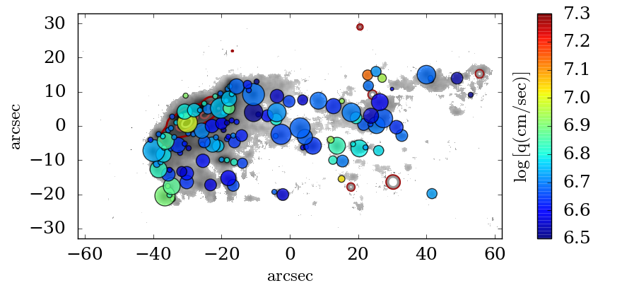
Figure 14: Metallicity (left) and $q$ ionization parameter (right) of the knots. The grey shaded area represents the $\rm H\alpha$ image.

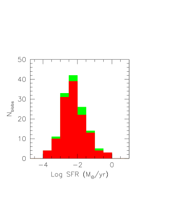
Figure 15: Left. SFR distribution of the “Star-forming” (red) and “Composite” (green) knots. The AGN-powered central knot has been excluded. Center. Distribution of gas densities of individual knots. Other $\sim 45$ knots not included in the plot have densities probably lower than the range shown here (see text). Right. Distribution of ionized gas masses of the individual knots plotted in middle panel.

7.5 Stellar history and star formation

The total SFR computed from the dust- and absorption-corrected $\rm H\alpha$ luminosity is 6.7 $M_{\odot}\,yr^{-1}$, of which 4.3/5.9 $M_{\odot}\,yr^{-1}$ within the inner/outer continuum isophotes. The SFR outside of the galaxy main body is therefore $\sim 1-2.5M_{\odot}\,yr^{-1}$. Subtracting the contribution from the regions that are classified as AGN or LINERS from the BPT diagram, the total SFR remains 5.6 $M_{\odot}\,yr^{-1}$.

The spatially resolved stellar history is reconstructed from SINOPSIS, which allows us to investigate how many stars were formed at each location during four logarithmically-spaced periods of time (Fig. 16).

The ongoing star formation activity (stars formed during the last $2\times 10^{7}yr$, top left panel in Fig. 16), is very intense along the east side of the disk, but is essentially absent in the easternmost stellar arm where the gas has already been totally stripped (cf. Fig. 5). Ongoing star formation is also present throughout the stripped gas, including the tails far out of the galaxy, with knots of higher than average SFR spread at different locations.

The recent star formation activity (between $2\times 10^{7}yr$ and $5.7\times 10^{8}yr$, top right panel) has a slightly different spatial distribution compared to the youngest stars: recent star formation was present also in the easternmost galaxy arm, a wide region of SF activity was present to the west of the galaxy body (X coordinates=-20 to 0), and the SFR in the tentacles was more rarefied. In agreement with this, inspecting the spectra in the easternmost galaxy arm shows typical post-starburst (k+a, Dressler et al., 1999, Poggianti et al. 1999) features, with no emission lines and extremely strong Balmer lines in absorption (rest frame $\rm H\beta\sim 10\AA$).

The distribution of older stars ($>\sim 6\times 10^{8}yr$) is drastically different, being mostly confined to the main galaxy body (two bottom panels of Fig. 16).

The different spatial distributions of stars of different ages indicate that the star formation in the stripped gas was ignited sometime during the last $\sim 5\times 10^{8}$yr.

As a consequence of the spatially-varying star formation history, the stellar luminosity-weighted age varies with position (Fig. 17). Overall, there is a clear age gradients from older to younger ages going from east to west, with a few noticeable exceptions: on the galaxy disk, there are some regions of very young ages, corresponding to the high SFR density regions in Fig. 16, that coincide with very intense H$\alpha$ surface brightness (cf. Fig. 5) and high metallicity (Fig. 10) whose emission is powered by star formation (Fig. 9). The tails have low LW ages, as expected given the star formation history of Fig. 16.

While the distribution of recent star formation is driven by the stripping of the gas, the stellar mass density distribution is dominated by the old stellar generations (Fig. 17, right). The mass density in the tails and in the stripped gas in general is very low, more than two orders of magnitude lower than in the galaxy disk (where the density is highest), and about an order of magnitude lower than in the outer regions of the disk.

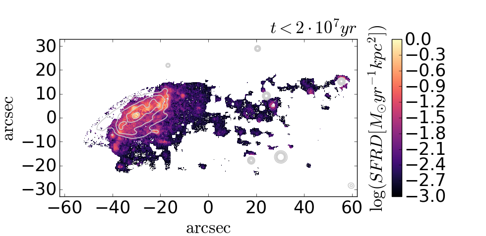
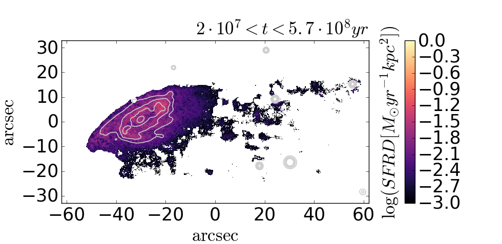
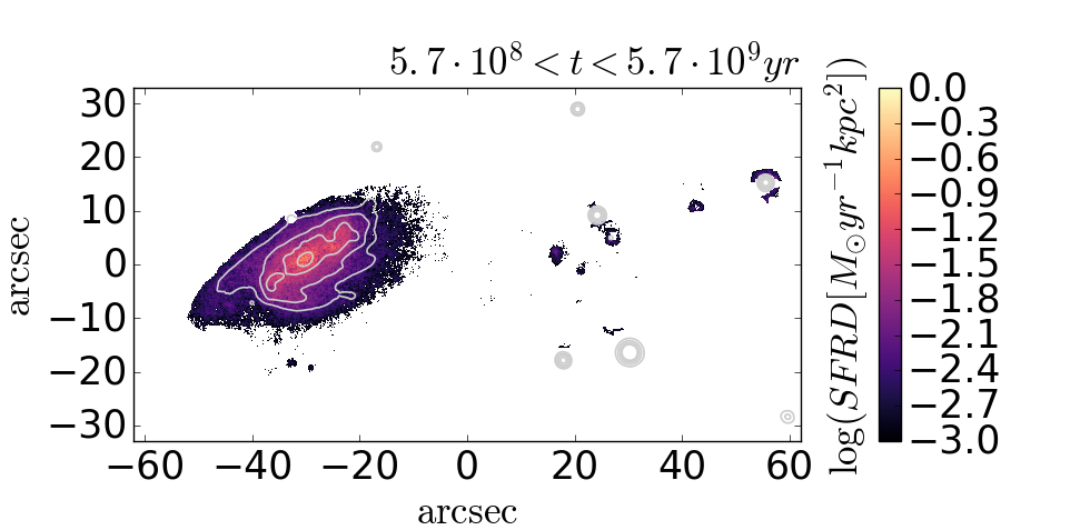
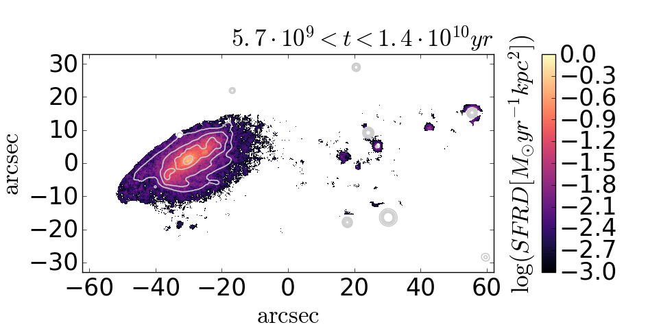
Figure 16: Stellar maps of different ages, illustrating the average star formation rate per $\rm kpc^{2}$ during the last $2\times 10^{7}yr$ (top left), between $2\times 10^{7}yr$ and $5.7\times 10^{8}yr$ (top right), $5.7\times 10^{8}yr$ and $5.7\times 10^{9}yr$ (bottom left) and $>5.7\times 10^{9}yr$ ago (bottom right). Contours in all panels are continuum isophotes as in Fig. 4.

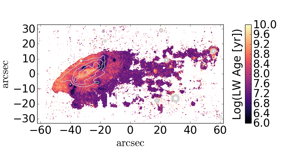
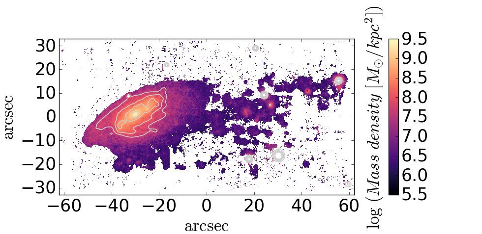
Figure 17: Left. Map of luminosity-weighted stellar age. Right: Stellar mass density map. Contours in both panels are continuum isophotes as in Fig. 4.

7.6 JO206 environment

IIZW108 is a poor galaxy cluster with an X-ray luminosity $L_{X}=1.09\times 10^{44}\,\rm erg\,s^{-1}$ (ROSAT 0.1-2.4 keV, Smith et al. 2004). In the literature (e.g. in SIMBAD and NED), it is commonly refereed to as a galaxy group, for its modest X-ray luminosity and temperature ($T_{X}=3.93\pm 0.1$ keV, Shang & Scharf 2009) and optical richness. According to previous studies, IIZW108 has little intracluster light and is undergoing major merging in its central regions, with four galaxies now in the process of building up the BCG (Edwards et al. 2016, see also Fig. 3). The only velocity dispersion estimates for this cluster are from WINGS and OMEGAWINGS: 549$\pm$42 $\rm km/s$ (Cava et al. 2009), and revised values of 611$\pm$38 $\rm km/s$ based on 171 spectroscopic members (Moretti et al. 2017) and 545/513${}^{+37}_{-35}\rm km/s$ based on 179 spectroscopic members including/excluding galaxies in substructures (Biviano et al. in prep.). Cluster mass and radius are estimated from the dynamical analysis of Biviano et al. (in prep.) with the MAMPOSSt technique (Mamon et al. 2013) to be $M_{200}=1.91^{+0.96}_{-0.45}\times 10^{14}\,M_{\sun}$ and $R_{200}=1.17^{+0.17}_{-0.10}\rm\,Mpc$.

The dynamical analysis of IIZW108 confirms that it has a highly significant substructure in the central region, and shows evidence for a few additional, less significant substructures, distributed from the north-east to the south-west of the cluster, as shown in Fig. 18 (see also Biviano et al. in prep.). However, there is no evidence for JO206 to reside in any of these substructures. On the contrary, this galaxy appears to have fallen recently into the cluster as an isolated galaxy.

JO206 is located in the most favorable conditions for ram pressure stripping within the cluster: it is at a small projected cluster-centric radius ($r_{cl}\sim 0.3R_{200}$ from the BCG), and it has a high differential velocity with respect to the cluster redshift ($\Delta v_{cl}\sim 800kms^{-1}\sim 1.5\sigma_{cl}$) (Fig. 18). We can compute the expected ram-pressure on JO206 by the ICM as $P_{ram}=\rho_{ICM}\times v_{cl}^{2}$ (Gunn & Gott 1972), where $\rho_{ICM}(r_{cl})$ is the radial density profile of the ICM. As we do not have a good estimate of $\rho_{ICM}(r_{cl})$ for IIZW108, we used the well-studied Virgo cluster as a close analogue (the clusters have very similar mass), assuming a smooth static ICM:

$$\rho_{{}_{ICM}}(r_{cl})=\rho_{0}\left[1+\left(\frac{r_{cl}}{r_{c}}\right)^{2}\right]^{-3\beta/2},$$ (4)

with core radius $r_{c}=13.4kpc$ , slope parameter $\beta=0.5$, and central density $\rho_{0}=4\times 10^{2}cm^{-3}$ (the same values used in Vollmer et al. 2001). At the projected $r_{cl}$ and line-of-sight velocity of JO206, we get a lower limit to the pressure:

$$P_{ram}=6\times 10^{-14}Nm^{-2}$$ (5)

We then compare the ram pressure of IIZW108 with the anchoring force of an idealized disk galaxy with the properties of JO206. The anchoring force of a disk galaxy $\Pi_{gal}=2\pi G\Sigma_{g}\Sigma_{s}$ is a function of the density profiles of the stars and the gas components ($\Sigma_{g}$ and $\Sigma_{s}$ respectively), that can be expressed as exponential functions:

$$\Sigma=(\frac{M_{d}}{2\pi r_{d}^{2}})e^{-r^{\prime}/r_{d}},$$ (6)

where $M_{d}$ is the disk mass, $r_{d}$ the disk scale-length and r the radial distance from the center of the galaxy. For the stellar component of JO206 we adopted a disk mass $M_{d,stars}=8.5\times 10^{10}M_{\odot}$, and a disk scale-length $r_{d,stars}=5.73$ kpc, obtained by fitting the light profile of the galaxy with GASPHOT (D’Onofrio et al. 2014). For the gas component we assumed a total mass $M_{d,gas}=0.1\times M_{d,stars}$, and scale-length $r_{d,gas}=1.7\times r_{d,stars}$ (Boselli & Gavazzi 2006).

At the centre of the galaxy ($r=0$) the anchoring force is too high for stripping to happen ($\Pi_{gal}(r=0)\simeq 10^{-11}Nm^{-2}$). The condition for stripping ($P_{ram}$/$\Pi_{gal}>1$) is only met at a radial distance of $r\simeq 20kpc\sim 2\times r_{d,gas}$ from the centre of the disk, which coincides very well with the “truncation radius” ($r_{t}$) measured from the extent of $\rm H{\alpha}$ emission (see e.g. Fig. 5). At $r=r_{t}$ the anchoring force drops to

$$\Pi_{gal}(r=r_{tr})\simeq 4\times 10^{-14}Nm^{-2}\sim 0.7\times P_{ram}$$ (7)

and the fraction of remaining gas mass can be computed as:

$$f=1+\left[e^{-r_{t}/r_{d}}\left(\frac{-r_{t}}{r_{d}}-1\right)\right]$$ (8)

This simplified calculation yields a gas mass fraction lost to the ICM wind of 15%. This amount of stripping happens at the combination of clustercentric distances and velocities shown by the blue lines in the right-hand panel of Fig. 18, where the condition $P_{ram}\simeq\Pi_{gal}(r=r_{tr})$ is met. The infalling galaxy has been approaching the cluster core moving from the right hand side of the plot to the left, and gaining absolute velocity (see e.g. Fig. 6 in Yoon et al. 2007). At the time of observation the galaxy is crossing the 15% stripping line, and it will continue to get stripped if it reaches lower $r_{cl}$.

We note that, although our calculation for JO206 supports ongoing ram-pressure stripping, there are several caveats to be considered (see discussion in e.g. Kenney et al. 2004 and Jaffé et al. 2015). First, the three-dimensional position and velocity of the galaxy are unknown, we use projected values. Second, in our calculations we assumed an idealized exponential disk interacting face-on with a static and homogeneous ICM. Simulations have shown however, that the intensity of ram-pressure stripping can be enhanced in cluster mergers (Vijayaraghavan & Ricker 2013) due to the presence of higher density clumps or shock waves, and that its efficiency varies with galaxy inclination (Abadi et al. 1999, Quillis et al. 2000, Vollmer et al. 2001). Finally, given the current lack of a direct measurement of the cold gas component of JO206, we used the extent of $\rm H\alpha$ to estimate the amount of gas stripped. It is yet to be tested with approved JVLA observations whether HI is more truncated than $\rm H\alpha$ in this jellyfish galaxy.

JO206 is therefore an example of a high mass galaxy undergoing strong ram pressure stripping in a poor, low-mass cluster. JO206 is not the only known jellyfish with these characteristics: NGC 4569 is also a quite massive ($10^{10.5}M_{\odot}$) galaxy in a $\sim 10^{14}M_{\odot}$ cluster (Virgo) (Boselli et al. 2016).

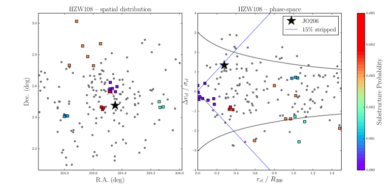
Figure 18: Left. Position on the sky of IIZW108 members (small black points) and non-members (small crosses), with large squares indicating the members of several substructures, color-coded according to the probability of these substructures to be random fluctuations (i.e. values close to zero indicate highly significant substructure detections, Biviano et al. in prep.). JO206 is the dark big star. The red cross is the BCG. Right. Phase-space diagram with symbols as in the left panel, assuming $\sigma=545\,\rm km/s$ and $R_{200}=1.17\rm\,Mpc$ (see text). Curves show the escape velocity in a Navarro, Frenk & White (1997) halo. The blue line corresponds to 15% of the total gas mass of JO206 stripped due to ram-pressure by the ICM in a Virgo-like cluster (see text for details).

8 Summary

GASP (GAs Stripping phenomena in galaxies with MUSE) is an ongoing ESO Large Program with the MUSE spectrograph on the VLT. This program started on October 1st 2015 and was allocated 120 hours over four semesters to observe 114 galaxies to study the causes and the effects of gas removal processes in galaxies. GASP galaxies were homogeneously selected in clusters and in the field from the WINGS, OMEGAWINGS and PM2GC surveys, and belong to dark matter haloes with masses covering over four orders of magnitude.

The main scientific drivers of GASP are a study of gas removal processes in galaxies in different environments, their effects for the star formation activity and quenching, the interplay between the gas conditions and the AGN activity, and the stellar and metallicity history of galaxies out to large radii prior to and in absence of gas removal.

The combination of large field-of-view, high sensitivity, large wavelength coverage and good spatial and spectral resolution of MUSE allow to peer into the outskirts and surroundings of a large sample of galaxies with different masses and environments. The MUSE data is capable to reveal the rich physics of the ionized gas external to galaxies and the stars that formed within it.

In this paper we have described the survey strategy and illustrated the main steps of the scientific analysis, showing their application to JO206, a rather rare example of a massive ($9\times 10^{10}M_{\odot}$) galaxy undergoing strong ram pressure stripping in a low mass cluster and forming $\sim 7M_{\odot}\,yr^{-1}$. Tails of stripped gas are visible out to 90 kpc from the galaxy disk. The gas is ionized mosty by in situ star formation, as new stars are formed in the tails. The gas tails are characterized both by regions of diffuse emission and bright knots, appearing to be giant HII regions and complexes, that retain a coherent rotation with the stars in the disk. The metallicity of the gas varies over an order of magnitude from metal-rich regions on one side of the disk, to very metal poor in some of the tails. The galaxy hosts an AGN, that is responsible for $\sim 15$% of the $\rm H\alpha$ ionization.

The MUSE data reveal how the stripping and the star formation activity and quenching have proceeded. The gas was stripped first from the easternmost arm, where star formation stopped during the last few $10^{8}$ yr. Star formation is still taking place in the disk, but about a third of the total SFR (having excluded the AGN) takes place outside of the main galaxy body, in the extraplanar gas and tails. Assuming a Chabrier IMF, 1-2 $M_{\odot}\,yr^{-1}$ are formed outside of the galaxy disk, and go to increase the intracluster light.

The first results shown in this and other papers of the series illustrate the power of the MUSE data to provide an exquisite view of the physical phenomena affecting the gas content of galaxies. GASP follow-up programs are undergoing to probe also the other gas phases and obtain a multiwavelength view of this sample. Ongoing APEX programs are yielding the CO amount in the disk and in the tails. Approved JVLA observations will provide the precious neutral gas information. Near-UV and far-UV data, as well as complementary X-ray data, are being obtained for a subset of GASP clusters with ASTROSAT (Subramaniam et al. 2016, Agrawal, P.C., 2006), while JWST will open the possibility to obtain an unprecedented view of the $H_{2}$ gas.

References

- Abadi et al. (1999) Abadi, M. G., Moore, B., & Bower, R. G. 1999, MNRAS, 308, 947
- Abramson et al. (2016) Abramson, A., Kenney, J., Crowl, H., & Tal, T. 2016, AJ, 152, 32
- Abramson et al. (2011) Abramson, A., Kenney, J. D. P., Crowl, H. H., et al. 2011, AJ, 141, 164
- Agrawal (2006) Agrawal, P. C. 2006, Advances in Space Research, 38, 2989
- Allen et al. (2015) Allen, J. T., Croom, S. M., Konstantopoulos, I. S., et al. 2015, MNRAS, 446, 1567
- Bacon et al. (2010) Bacon, R., Accardo, M., Adjali, L., et al. 2010, in Proc. SPIE, Vol. 7735, Ground-based and Airborne Instrumentation for Astronomy III, 773508
- Baldwin et al. (1981) Baldwin, J. A., Phillips, M. M., & Terlevich, R. 1981, PASP, 93, 5
- Balogh et al. (2000) Balogh, M. L., Navarro, J. F., & Morris, S. L. 2000, ApJ, 540, 113
- Barnes & Hernquist (1992) Barnes, J. E., & Hernquist, L. 1992, ARA&A, 30, 705
- Bell et al. (2004) Bell, E. F., Wolf, C., Meisenheimer, K., et al. 2004, ApJ, 608, 752
- Bellhouse (2017) Bellhouse, C., et al. 2017, ApJ in press (Paper II), arXiv 1704.05087
- Birnboim & Dekel (2003) Birnboim, Y., & Dekel, A. 2003, MNRAS, 345, 349
- Bolatto et al. (2013) Bolatto, A. D., Warren, S. R., Leroy, A. K., et al. 2013, Nature, 499, 450
- Boselli et al. (2014) Boselli, A., Cortese, L., Boquien, M., et al. 2014, A&A, 564, A66
- Boselli & Gavazzi (2006) Boselli, A., & Gavazzi, G. 2006, PASP, 118, 517
- Boselli et al. (1997) Boselli, A., Gavazzi, G., Lequeux, J., et al. 1997, A&A, 327, 522
- Boselli et al. (2016) Boselli, A., Cuillandre, J. C., Fossati, M., et al. 2016, A&A, 587, A68
- Bouché et al. (2013) Bouché, N., Murphy, M. T., Kacprzak, G. G., et al. 2013, Science, 341, 50
- Bournaud et al. (2011) Bournaud, F., Dekel, A., Teyssier, R., et al. 2011, ApJ, 741, L33
- Bressan (2012) Bressan, A., et al. 2012, MNRAS, 427, 127
- Brinchmann et al. (2004) Brinchmann, J., Charlot, S., White, S. D. M., et al. 2004, MNRAS, 351, 1151
- Bundy et al. (2015) Bundy, K., Bershady, M. A., Law, D. R., et al. 2015, ApJ, 798, 7
- Byrd & Valtonen (1990) Byrd, G., & Valtonen, M. 1990, ApJ, 350, 89
- Calvi et al. (2012) Calvi, R., Poggianti, B. M., Fasano, G., & Vulcani, B. 2012, MNRAS, 419, L14
- Calvi et al. (2011) Calvi, R., Poggianti, B. M., & Vulcani, B. 2011, MNRAS, 416, 727
- Cantalupo et al. (2014) Cantalupo, S., Arrigoni-Battaia, F., Prochaska, J. X., Hennawi, J. F., & Madau, P. 2014, Nature, 506, 63
- Cantalupo et al. (2012) Cantalupo, S., Lilly, S. J., & Haehnelt, M. G. 2012, MNRAS, 425, 1992
- Cappellari & Copin (2003) Cappellari, M., & Copin, Y. 2003, MNRAS, 342, 345
- Cappellari & Emsellem (2004) Cappellari, M., & Emsellem, E. 2004, PASP, 116, 138
- Cardelli et al. (1989) Cardelli, J. A., Clayton, G. C., & Mathis, J. S. 1989, ApJ, 345, 245
- Cava et al. (2009) Cava, A., Bettoni, D., Poggianti, B. M., et al. 2009, A&A, 495, 707
- Cayatte et al. (1990) Cayatte, V., van Gorkom, J. H., Balkowski, C., & Kotanyi, C. 1990, AJ, 100, 604
- Chabrier (2003) Chabrier, G. 2003, PASP, 115, 763
- Christensen et al. (2016) Christensen, C. R., Davé, R., Governato, F., et al. 2016, ApJ, 824, 57
- Chung et al. (2009) Chung, A., van Gorkom, J. H., Kenney, J. D. P., Crowl, H., & Vollmer, B. 2009, AJ, 138, 1741
- Cicone et al. (2014) Cicone, C., Maiolino, R., Sturm, E., et al. 2014, A&A, 562, A21
- Condon et al. (1998) Condon, J. J., Cotton, W. D., Greisen, E. W., et al. 1998, AJ, 115, 1693
- Cortese et al. (2004) Cortese, L., Gavazzi, G., Boselli, A., & Iglesias-Paramo, J. 2004, A&A, 416, 119
- Cortese et al. (2007) Cortese, L., Marcillac, D., Richard, J., et al. 2007, MNRAS, 376, 157
- Cowie & Songaila (1977) Cowie, L. L., & Songaila, A. 1977, Nature, 266, 501
- Cresci et al. (2015) Cresci, G., Marconi, A., Zibetti, S., et al. 2015, A&A, 582, A63
- Dekel & Birnboim (2006) Dekel, A., & Birnboim, Y. 2006, MNRAS, 368, 2
- Dekel et al. (2009) Dekel, A., Birnboim, Y., Engel, G., et al. 2009, Nature, 457, 451
- Diehl & Statler (2006) Diehl, S., & Statler, T. S. 2006, MNRAS, 368, 497
- Di Matteo et al. (2005) Di Matteo, T., Springel, V., & Hernquist, L. 2005, Nature, 433, 604
- D’Onofrio et al. (2014) D’Onofrio, M., Bindoni, D., Fasano, G., et al. 2014, A&A, 572, A87
- Dopita et al. (2013) Dopita, M. A., Sutherland, R. S., Nicholls, D. C., Kewley, L. J., & Vogt, F. P. A. 2013, ApJS, 208, 10
- Dopita et al. (2006) Dopita, M. A., Fischera, J., Sutherland, R. S., et al. 2006, ApJ, 647, 244
- Dressler et al. (2009) Dressler, A., Rigby, J., Oemler, Jr., A., et al. 2009, ApJ, 693, 140
- Dressler et al. (1999) Dressler, A., Smail, I., Poggianti, B. M., et al. 1999, ApJS, 122, 51
- Driver et al. (2005) Driver, S. P., Liske, J., Cross, N. J. G., De Propris, R., & Allen, P. D. 2005, MNRAS, 360, 81
- Ebeling et al. (2000) Ebeling, H., Edge, A. C., Allen, S. W., et al. 2000, MNRAS, 318, 333
- Ebeling et al. (1998) Ebeling, H., Edge, A. C., Bohringer, H., et al. 1998, MNRAS, 301, 881
- Ebeling et al. (2014) Ebeling, H., Ma, C.-J., & Barrett, E. 2014, ApJS, 211, 21
- Ebeling et al. (1996) Ebeling, H., Voges, W., Bohringer, H., et al. 1996, MNRAS, 281, 799
- Edwards et al. (2016) Edwards, L. O. V., Alpert, H. S., Trierweiler, I. L., Abraham, T., & Beizer, V. G. 2016, MNRAS, 461, 230
- Efstathiou & Silk (1983) Efstathiou, G., & Silk, J. 1983, Fund. Cosmic Phys., 9, 1
- Erb (2015) Erb, D. K. 2015, Nature, 523, 169
- Fabian (2012) Fabian, A. C. 2012, ARA&A, 50, 455
- Fasano et al. (2006) Fasano, G., Marmo, C., Varela, J., et al. 2006, A&A, 445, 805
- Fasano et al. (2012) Fasano, G., Vanzella, E., Dressler, A., et al. 2012, MNRAS, 420, 926
- Ferguson & Mackey (2016) Ferguson, A. M. N., & Mackey, A. D. 2016, Tidal Streams in the Local Group and Beyond, 420, 191
- Ferland (2013) Ferland, G.J., 2013, MxAA, 49, 137
- Feruglio et al. (2010) Feruglio, C., Maiolino, R., Piconcelli, E., et al. 2010, A&A, 518, L155
- Fossati et al. (2016) Fossati, M., Fumagalli, M., Boselli, A., et al. 2016, MNRAS, 455, 2028
- Fossati et al. (2012) Fossati, M., Gavazzi, G., Boselli, A., & Fumagalli, M. 2012, A&A, 544, A128
- Fritz et al. (2007) Fritz, J., Poggianti, B. M., Bettoni, D., et al. 2007, A&A, 470, 137
- Fritz et al. (2011) Fritz, J., Poggianti, B. M., Cava, A., et al. 2011, A&A, 526, A45
- Fritz et al. (2014) —. 2014, A&A, 566, A32
- Fritz (2017) Fritz, J., et al. 2017, ApJ, submitted, arXiv 1704.05088
- Fumagalli et al. (2014) Fumagalli, M., Fossati, M., Hau, G. K. T., et al. 2014, MNRAS, 445, 4335
- Fumagalli et al. (2011) Fumagalli, M., Gavazzi, G., Scaramella, R., & Franzetti, P. 2011, A&A, 528, A46
- Gavazzi et al. (2002) Gavazzi, G., Bonfanti, C., Sanvito, G., Boselli, A., & Scodeggio, M. 2002, ApJ, 576, 135
- Genzel et al. (2014) Genzel, R., Förster Schreiber, N. M., Rosario, D., et al. 2014, ApJ, 796, 7
- Gerhard et al. (2002) Gerhard, O., Arnaboldi, M., Freeman, K. C., & Okamura, S. 2002, ApJ, 580, L121
- Girardi et al. (2000) Girardi, L., Bressan, A., Bertelli, G., & Chiosi, C. 2000, A&AS, 141, 371
- Guglielmo et al. (2015) Guglielmo, V., Poggianti, B. M., Moretti, A., et al. 2015, MNRAS, 450, 2749
- Gullieuszik et al. (2015) Gullieuszik, M., Poggianti, B., Fasano, G., et al. 2015, A&A, 581, A41
- Gullieuszik (2017) Gullieuszik, A., et al., ApJ submitted
- Gunn & Gott (1972) Gunn, J. E., & Gott, III, J. R. 1972, ApJ, 176, 1
- Haynes et al. (1984) Haynes, M. P., Giovanelli, R., & Chincarini, G. L. 1984, ARA&A, 22, 445
- Hess & Wilcots (2013) Hess, K. M., & Wilcots, E. M. 2013, AJ, 146, 124
- Hester & Tasitsiomi (2010) Hester, J. A., & Tasitsiomi, A. 2010, ApJ, 715, 342
- Hopkins et al. (2003) Hopkins, A. M., Miller, C. J., Nichol, R. C., et al. 2003, ApJ, 599, 971
- Hopkins et al. (2006) Hopkins, P. F., Somerville, R. S., Hernquist, L., et al. 2006, ApJ, 652, 864
- Jáchym et al. (2014) Jáchym, P., Combes, F., Cortese, L., Sun, M., & Kenney, J. D. P. 2014, ApJ, 792, 11
- Jáchym et al. (2013) Jáchym, P., Kenney, J. D. P., Ržuička, A., et al. 2013, A&A, 556, A99
- Jaffé et al. (2015) Jaffé, Y. L., Smith, R., Candlish, G. N., et al. 2015, MNRAS, 448, 1715
- Kapferer et al. (2008) Kapferer, W., Kronberger, T., Ferrari, C., Riser, T., & Schindler, S. 2008, MNRAS, 389, 1405
- Kauffmann et al. (2016) Kauffmann, G., Borthakur, S., & Nelson, D. 2016, MNRAS, 462, 3751
- Kauffmann et al. (2004) Kauffmann, G., White, S. D. M., Heckman, T. M., et al. 2004, MNRAS, 353, 713
- Kauffmann et al. (2003) Kauffmann, G., Heckman, T. M., Tremonti, C., et al. 2003, MNRAS, 346, 1055
- Kenney et al. (2015) Kenney, J. D. P., Abramson, A., & Bravo-Alfaro, H. 2015, AJ, 150, 59
- Kenney et al. (2014) Kenney, J. D. P., Geha, M., Jáchym, P., et al. 2014, ApJ, 780, 119
- Kenney & Koopmann (1999) Kenney, J. D. P., & Koopmann, R. A. 1999, AJ, 117, 181
- Kenney et al. (2004) Kenney, J. D. P., van Gorkom, J. H., & Vollmer, B. 2004, AJ, 127, 3361
- Kenney & Young (1989) Kenney, J. D. P., & Young, J. S. 1989, ApJ, 344, 171
- Kennicutt (1998) Kennicutt, Jr., R. C. 1998, ARA&A, 36, 189
- Kereš et al. (2005) Kereš, D., Katz, N., Weinberg, D. H., & Davé, R. 2005, MNRAS, 363, 2
- Kewley et al. (2006) Kewley, L. J., Groves, B., Kauffmann, G., & Heckman, T. 2006, MNRAS, 372, 961
- Kewley et al. (2001) Kewley, L. J., Heisler, C. A., Dopita, M. A., & Lumsden, S. 2001, ApJS, 132, 37
- King & Pounds (2015) King, A., & Pounds, K. 2015, ARA&A, 53, 115
- Kormendy & Ho (2013) Kormendy, J., & Ho, L. C. 2013, ARA&A, 51, 511
- Larson et al. (1980) Larson, R. B., Tinsley, B. M., & Caldwell, C. N. 1980, ApJ, 237, 692
- Liske et al. (2003) Liske, J., Lemon, D. J., Driver, S. P., Cross, N. J. G., & Couch, W. J. 2003, MNRAS, 344, 307
- Madau & Dickinson (2014) Madau, P., & Dickinson, M. 2014, eprint arXiv, 1403, 7
- Mamon et al. (2013) Mamon, G. A., Biviano, A., & Boué, G. 2013, MNRAS, 429, 3079
- Marasco et al. (2016) Marasco, A., Crain, R. A., Schaye, J., et al. 2016, MNRAS, 461, 2630
- Markwardt (2009) Markwardt, C. B. 2009, in Astronomical Society of the Pacific Conference Series, Vol. 411, Astronomical Data Analysis Software and Systems XVIII, ed. D. A. Bohlender, D. Durand, & P. Dowler, 251
- Martini et al. (2006) Martini, P., Kelson, D. D., Kim, E., Mulchaey, J. S., & Athey, A. A. 2006, ApJ, 644, 116
- Marziani et al. (2017) Marziani, P., D’Onofrio, M., Bettoni, D., et al. 2017, A&A, 599, A83
- Mayer et al. (2008) Mayer, L., Governato, F., & Kaufmann, T. 2008, Advanced Science Letters, 1, 7
- McPartland et al. (2016) McPartland, C., Ebeling, H., Roediger, E., & Blumenthal, K. 2016, MNRAS, 455, 2994
- Merluzzi et al. (2016) Merluzzi, P., Busarello, G., Dopita, M. A., et al. 2016, MNRAS, 460, 3345
- Merluzzi et al. (2013) —. 2013, MNRAS, 429, 1747
- Miller et al. (2003) Miller, C. J., Nichol, R. C., Gómez, P. L., Hopkins, A. M., & Bernardi, M. 2003, ApJ, 597, 142
- Moore et al. (1996) Moore, B., Katz, N., Lake, G., Dressler, A., & Oemler, A. 1996, Nature, 379, 613
- Moretti et al. (2014) Moretti, A., Poggianti, B. M., Fasano, G., et al. 2014, A&A, 564, A138
- Moretti et al. (2017) Moretti, A., Gullieuszik, M., Poggianti, B., et al. 2017, A&A, 599, A81
- Moretti (2017) Moretti, A., et al. 2017, submitted
- Navarro et al. (1996) Navarro, J. F., Frenk, C. S., & White, S. D. M. 1996, ApJ, 462, 563
- Noeske et al. (2007) Noeske, K. G., Weiner, B. J., Faber, S. M., et al. 2007, ApJ, 660, L43
- Nulsen (1982) Nulsen, P. E. J. 1982, MNRAS, 198, 1007
- Omizzolo et al. (2014) Omizzolo, A., Fasano, G., Reverte Paya, D., et al. 2014, A&A, 561, A111
- Osterbrock & Ferland (2006) Osterbrock, D. E., & Ferland, G. J. 2006, Astrophysics of gaseous nebulae and active galactic nuclei
- Owers et al. (2012) Owers, M. S., Couch, W. J., Nulsen, P. E. J., & Randall, S. W. 2012, ApJ, 750, L23
- Paccagnella et al. (2016) Paccagnella, A., Vulcani, B., Poggianti, B. M., et al. 2016, ApJ, 816, L25
- Peterson & Fabian (2006) Peterson, J. R., & Fabian, A. C. 2006, Phys. Rep., 427, 1
- Poggianti et al. (1999) Poggianti, B. M., Smail, I., Dressler, A., et al. 1999, ApJ, 518, 576
- Poggianti et al. (2016) Poggianti, B. M., Fasano, G., Omizzolo, A., et al. 2016, AJ, 151, 78
- Poggianti (2017) Poggianti, B.M., et al. 2017, submitted
- Popesso & Biviano (2006) Popesso, P., & Biviano, A. 2006, A&A, 460, L23
- Proxauf et al. (2014) Proxauf, B., Öttl, S., & Kimeswenger, S. 2014, A&A, 561, A10
- Quilis et al. (2000) Quilis, V., Moore, B., & Bower, R. 2000, Science, 288, 1617
- Rasmussen et al. (2006) Rasmussen, J., Ponman, T. J., & Mulchaey, J. S. 2006, MNRAS, 370, 453
- Rasmussen et al. (2008) Rasmussen, J., Ponman, T. J., Verdes-Montenegro, L., Yun, M. S., & Borthakur, S. 2008, MNRAS, 388, 1245
- Rawle et al. (2014) Rawle, T. D., Altieri, B., Egami, E., et al. 2014, MNRAS, 442, 196
- Roediger (2009) Roediger, E. 2009, Astronomische Nachrichten, 330, 888
- Roediger & Brüggen (2007) Roediger, E., & Brüggen, M. 2007, MNRAS, 380, 1399
- Roediger et al. (2014) Roediger, E., Brüggen, M., Owers, M. S., Ebeling, H., & Sun, M. 2014, MNRAS, 443, L114
- Sabater et al. (2015) Sabater, J., Best, P. N., & Heckman, T. M. 2015, MNRAS, 447, 110
- Sánchez et al. (2012) Sánchez, S. F., Kennicutt, R. C., Gil de Paz, A., et al. 2012, A&A, 538, A8
- Sancisi et al. (2008) Sancisi, R., Fraternali, F., Oosterloo, T., & van der Hulst, T. 2008, A&A Rev., 15, 189
- Schlafly & Finkbeiner (2011) Schlafly, E. F., & Finkbeiner, D. P. 2011, ApJ, 737, 103
- Shang & Scharf (2009) Shang, C., & Scharf, C. 2009, ApJ, 690, 879
- Sharp & Bland-Hawthorn (2010) Sharp, R. G., & Bland-Hawthorn, J. 2010, ApJ, 711, 818
- Smith et al. (2010) Smith, R. J., Lucey, J. R., Hammer, D., et al. 2010, MNRAS, 408, 1417
- Soto et al. (2016) Soto, K. T., Lilly, S. J., Bacon, R., Richard, J., & Conseil, S. 2016, MNRAS, 458, 3210
- Steidel et al. (2010) Steidel, C. C., Erb, D. K., Shapley, A. E., et al. 2010, ApJ, 717, 289
- Storey & Zeippen (2000) Storey, P. J., & Zeippen, C. J. 2000, MNRAS, 312, 813
- Sun et al. (2010) Sun, M., Donahue, M., Roediger, E., et al. 2010, ApJ, 708, 946
- Tonnesen & Bryan (2012) Tonnesen, S., & Bryan, G. L. 2012, MNRAS, 422, 1609
- Tonnesen & Stone (2014) Tonnesen, S., & Stone, J. 2014, ApJ, 795, 148
- Valentinuzzi et al. (2009) Valentinuzzi, T., Woods, D., Fasano, G., et al. 2009, A&A, 501, 851
- Varela et al. (2009) Varela, J., D’Onofrio, M., Marmo, C., et al. 2009, A&A, 497, 667
- Vazdekis et al. (2010) Vazdekis, A., Sánchez-Blázquez, P., Falcón-Barroso, J., et al. 2010, MNRAS, 404, 1639
- Veilleux et al. (2005) Veilleux, S., Cecil, G., & Bland-Hawthorn, J. 2005, ARA&A, 43, 769
- Verdes-Montenegro et al. (2001) Verdes-Montenegro, L., Yun, M. S., Williams, B. A., et al. 2001, A&A, 377, 812
- Vijayaraghavan & Ricker (2013) Vijayaraghavan, R., & Ricker, P. M. 2013, MNRAS, 435, 2713
- Vogelsberger et al. (2014) Vogelsberger, M., Genel, S., Springel, V., et al. 2014, Nature, 509, 177
- Voges et al. (1999) Voges, W., Aschenbach, B., Boller, T., et al. 1999, A&A, 349, 389
- Vollmer (2013) Vollmer, B. 2013, The Influence of Environment on Galaxy Evolution, ed. T. D. Oswalt & W. C. Keel, 207
- Vollmer et al. (2001) Vollmer, B., Cayatte, V., Balkowski, C., & Duschl, W. J. 2001, ApJ, 561, 708
- Vollmer et al. (2010) Vollmer, B., Soida, M., Chung, A., et al. 2010, A&A, 512, A36
- Vollmer et al. (2012) Vollmer, B., Soida, M., Braine, J., et al. 2012, A&A, 537, A143
- von der Linden et al. (2010) von der Linden, A., Wild, V., Kauffmann, G., White, S. D. M., & Weinmann, S. 2010, MNRAS, 404, 1231
- Vulcani et al. (2015) Vulcani, B., Poggianti, B. M., Fritz, J., et al. 2015, ApJ, 798, 52
- Wagg et al. (2014) Wagg, J., Carilli, C. L., Aravena, M., et al. 2014, ApJ, 783, 71
- White & Rees (1978) White, S. D. M., & Rees, M. J. 1978, MNRAS, 183, 341
- Yagi et al. (2013) Yagi, M., Gu, L., Fujita, Y., et al. 2013, ApJ, 778, 91
- Yagi et al. (2010) Yagi, M., Yoshida, M., Komiyama, Y., et al. 2010, AJ, 140, 1814
- Yoon (2007) Yoon, et al. 2007, ApJ, 838, 81
- Yoshida et al. (2012) Yoshida, M., Yagi, M., Komiyama, Y., et al. 2012, ApJ, 749, 43
- Yoshida et al. (2008) —. 2008, ApJ, 688, 918