The composition of Solar system asteroids and Earth/Mars moons, and the Earth-Moon composition similarity

Abstract

In the typical giant-impact scenario for the formation of the Moon, most of the Moon’s material originates from the impactor. Any Earth-impactor composition difference should, therefore, correspond to a comparable Earth-Moon composition difference. Analysis of Moon rocks shows a close Earth-Moon composition similarity, posing a challenge for the giant-impact scenario, given that impactors were thought to significantly differ in composition from the planets they impact. However, our recent analysis of 40 planet formation simulations has shown that the composition of impactors could be very similar to that of the planets they impact. Moreover, the difference in Earth-Moon–like systems is consistent with observations of $\Delta^{17}O<15$ppm for a significant fraction of the cases, thereby potentially resolving the composition similarity challenge. Here we use a larger set of 140 simulations and improved statistical analysis to further explore this issue. We find that in 4.9%-18.2% (1.9%-6.7%) of the cases the resulting composition of the Moon is consistent with observations of $\Delta^{17}O<15$ppm ($\Delta^{17}O<6$ ppm). These findings reaffirm our original results at higher statistical level and suggest that the Earth-Moon composition similarity could be resolved to arise from the primordial Earth-impactor composition similarity. Note that although we find the likelihood for the suggested competing model of very high mass-ratio impacts (producing significant Earth-impactor composition mixing) to be comparable ($<6.7\%$), this scenario also requires additional fine-tuned requirements of a very fast spinning Earth. Using the same simulations we also explore the composition of giant-impact formed Mars’ moons as well as Vesta-like asteroids. We predict that the Mars-moon composition difference should be large, but smaller than expected if the moons are captured asteroids. Finally, we find that the left-over planetesimals (‘asteroids’) in our simulations are frequently scattered far away from their initial positions, thus potentially explaining the mismatch between the current position and composition of the Vesta asteroid.

1 Introduction

The Moon is thought to be the result of a relatively low-velocity, oblique impact (Canup & Asphaug, 2001) between the proto-Earth and a Mars sized planetary embryo, Theia, that happened in the latest stages of the Earth assembly (Agnor et al., 1999; Jacobson & Morbidelli, 2014).
Precise isotopic measurement of lunar rocks, brought back by the Apollo missions, showed that the Moon has an isotopic composition almost indistinguishable from that of the Earth for various elements (O, Ti, Cr, W, K; Ringwood, 1986; Lugmair & Shukolyukov, 1998; Wiechert et al., 2001; Touboul et al., 2007; Zhang et al., 2012; Herwartz et al., 2014; Young et al., 2016; Jacobsen, 2005; Touboul et al., 2007). In particular, the oxygen isotope composition is characterised by a mutual difference $\Delta^{17}O=12\pm 3$ppm (Herwartz et al., 2014) or possibly smaller ($-1\pm 5$ppm), as recently found by Young et al. (2016) analysing different rock samples. However, since objects in the Solar System have significantly different compositions (e.g. Mars, Vesta), it is difficult to explain the Earth-Moon similarity in the giant-impact scenario in which most of the Moon material originates from the impactor. Solutions to this conundrum through strong mixing during the encounter (Ćuk & Stewart, 2012; Canup, 2012) require many ad-hoc assumptions for the impact, in particular extremely high spin for the proto-Earth, and fine-tuned conditions (Jacobson & Morbidelli, 2014). High angular momentum impacts could explain the potassium chemical and isotopic composition of the Moon as shown by Wang & Jacobsen (2016). The origins of the Solar system structure, and in particular the low mass of Mars are still debated. Making use of one of the suggested scenarios which may successfully explain Mars origin (Grand Tack; Walsh et al. 2011; but see difficulties with the model, e.g. D’Angelo & Marzari 2012; Bromley & Kenyon 2017), Young et al. (2016) found that the proto-Earth and Theia are likely to differ at the 0.1‰ level, and they therefore also suggested that a strong mixing following a high energy, high angular momentum impact in required to explain the Earth-Moon composition similarity. However, as recently shown by Rufu et al. (2017), such high spin is highly unlikely because angular momentum is efficiently removed through material ejected during the impact. Other models for low-mass mars, not involving migration (e.g. Bromley & Kenyon, 2017) are yet to be tested using Moon formation models. It is also possible that a a paradigm shift in regard to the Moon origin is required.
Using elements with distinct affinities for metals to trace the composition of material accreting to form the Earth at different times, Dauphas (2017) found that the Earth and Theia probably had similar chemical composition, thereby relaxing the constraints on the giant impact scenario.
The probability of an impact between two similar bodies, in the standard giant-impact scenario, has been explored using simulations of rocky planets formation. Assuming that the composition is a function of the initial distance of planetesimals and planetary embryos from the Sun and analysing the impact history of each planet, it is possible to obtain the mass-weighted composition of planets and the last impactors that could have formed the Moon. One can then compare the Earth and the Moon compositions in the simulations (see Kaib & Cowan, 2015a; Mastrobuono-Battisti et al., 2015; Kaib & Cowan, 2015b).
Here we extend previous findings using a larger set of simulations and applying an improved statistical analysis similar to the one described by Kaib & Cowan (2015a) and Kaib & Cowan (2015b), but extend it as to now also consider the statistical errors, in order to better asses the composition similarities of the Earth and the Moon. Such analysis can later be extended to Solar system and moon formation models beyond those considered here.

Moreover, we study the composition of Mars and its moons, and explore the composition of Solar system asteroids such as Vesta. Mars moons Phobos and Deimos have indeed been reconsidered as the result of a giant impact (Craddock, 2011; Citron et al., 2015) and Vesta is another interesting and peculiar object in our Solar System, showing a large discrepancy between its distance to the Sun and its composition relative to the Earth and Mars.
The paper is organised as follows: in Section 2 we describe the simulations and the analysis we performed. Our results are illustrated Section 3 and in Section 4 we summarise the main outcomes and draw our conclusions.

2 Methods

2.1 $N$-body simulations

Detailed $N$-body simulations of rocky planets formation have been recently used to study the composition of the Moon (Pahlevan & Stevenson, 2007; Mastrobuono-Battisti et al., 2015; Kaib & Cowan, 2015a, b; Young et al., 2016). Analysing only one simulation with 150 particles and considering all the impactors on every planet Pahlevan & Stevenson (2007) concluded that their composition was too different to explain the Earth-Moon similarity. In Mastrobuono-Battisti et al. (2015), hereafter Paper I, we used a suite of 40 $N$-body simulations with different initial conditions (see Raymond et al., 2009), to compare the composition of the planets formed with that of the relative last massive impactor. Our analysis led to a probability of compatibility between the Earth and Theia between 20% and 40%, depending on the degree of mixing allowed (from 0% to 40% of proto-Earth material contributing to the circumterrestrial disk). This hints to a general tendency for impactors and targets to have more similar compositions than different planets. Kaib & Cowan (2015a) used another set of 150 similar simulations and, with an analogous analysis, they obtained less than 5% chances to have an impact between similar bodies. Including the possibility of mixing and a statistical analysis based on bootstrapping, Kaib & Cowan (2015b) found that the fraction of Theia analogs consistent with the canonical giant impact hypothesis is in the 5%-8% range. The differences between the results obtained in these papers are mostly due to the choice of the analogs. In Paper I the order of the planets has been used to identify the Earth and Mars analogs (the third and forth planet in the system, respectively); moreover all the planets and last impactors where taken into account. Kaib & Cowan (2015a, b) adopted the identification criteria described in Section 2.2 and considered only the impactors on Earth’s analogs.

We used the set of 40 simulations (set I) used in Paper I combined with additional 100 simulations (set II) with similar initial conditions analysed in Kaib & Cowan (2015a, b) (this latter set of simulations is publicly available). The simulations, performed using Mercury code (Chambers, 1999), reproduce the latest stages of planetary formation following the birth of Jupiter and Saturn, after all the gas has been dissipated from the system or accreted by the giants (see Raymond et al., 2013, for a recent review). Set I and II include respectively eight and two ensembles with different initial conditions.

Simulations in set I begin from a disk of 85-90 planetary embryos and 1000-2000 planetesimals distributed between $0.5$ and $4.5$ au (see Raymond et al., 2009, for more details). In brief, in 12 simulations Jupiter and Saturn are mutually inclined with an angle of $0.5^{\circ}$ and orbit the Sun with semi-major axes of $a_{J}=5.45$ au for Jupiter and $a_{S}=8.18$ au for Saturn. In 8 of those simulations the orbits are circular (cjs), while in the other 4 they are slightly eccentric with $e_{J}=0.02$ for Jupiter and $e_{S}=0.03$ for Saturn (cjsecc). In 12 additional simulations Jupiter and Saturn are located in their current positions (5.25 and 9.54 au), with mutual inclination of $1.5^{\circ}$ and eccentricities $e_{J}=e_{S}=0.1$ or $e_{J}=0.07$ and $e_{S}=0.08$ (eejs). In 8 runs Raymond et al. (2009) adopted orbital parameters similar to the observed ones ($a_{J}=5.25$au and $e_{J}=0.05$, $a_{S}=9.54$ and $e_{S}=0.06$) with mutual inclination of $1.5^{\circ}$ (ejs). Four additional simulations have Jupiter and Saturn with $a_{J}=5.43$ au and $a_{S}=7.30$ au, $e_{J}=0.07$, $e_{S}=0.01$ and mutual inclination of $0.2^{\circ}$ (jres) and the last four are performed with the same semi-major axis and $e_{J}=0.07=e_{S}=0.03$ (jresecc).

All simulations in set II (see details in Kaib & Cowan, 2015a) consist of 1000 planetesimals and 100 planetary embryos extending between $0.5$ and $4.0$ pc. In 50 simulations, Jupiter and Saturn are on nearly circular ($e<0.01$) orbits with the current radius (cjsII), while in the other 50 runs Jupiter and Saturn are on orbits with small eccentricity ($e_{J}=e_{S}=0.1$) and with their observed semi-major axis (ejsII) .
In both set I and set II a time-step of 6 days has been used and each system has been evolved for 200Myr. Embryos and planetesimals collide with each other while orbiting the Sun, producing 3-4 rocky planets by the end of each simulation and leaving behind some not accreted planetesimals. The resulting planetary systems are similar to our Solar system. We note, however, that none of the simulations, in either set, is able to correctly reproduce the Solar System properties accurately; nevertheless those are among the best simulations available at the moment. In every run, the collisions experienced by each embryo are recorded and can be used to map the feeding zone of each planet that form in any system.

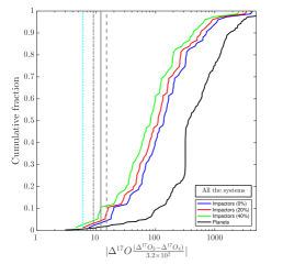
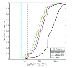
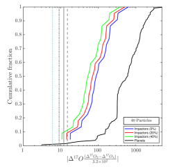
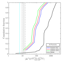
Figure 1: The cumulative distribution of the absolute $\Delta^{17}O$ differences between Earth analogs and Theia analogs, compared with the differences between planets in the same system (black), obtained from the raw simulations. Blue, red and green lines correspond to the cases of 0%, 20% and 40% contribution of material from the planet to a moon formed from these impacts, respectively. The vertical grey lines depict the $\Delta^{17}O$ difference of the Earth-Moon system (dot-dashed and dashed lines for $\pm\sigma$ around the mean value; central solid line). The cyan dot vertical line depicts the more recent $1\sigma$ estimate for the same difference (see Young et al., 2016). The same plot is shown for all the systems (top left panel), regardless of the number of particles that contributed to their formation, and planets and last impactors composed of a minimum of 10, 20, 30, 40 and 50 particles.

2.2 Earth and Mars analogs

Following Kaib & Cowan (2015a, b) we identify an Earth analog as the planet that have a final semi-major axis between $0.8$ and $1.2$ au and mass $m>0.5M_{\oplus}$. Mars analog is defined as the next planet to the Earth with $m>0.05M_{\oplus}$ while Theia analog is the last body with $m>0.1M_{\oplus}$ that hit the Earth analog. These conditions are fulfilled in 75 out of 140 simulations (22 from set I and 53 from set II).
The analog of the last Mars impactor is the last planetary embryo that struck the planet and whose mass is larger than 0.01 times the mass of Mars. This choice leaves us with 79 simulations useful for analysis (25 from set I and 54 from set II).
In order to maximise the number of simulations that can be analysed, we did not constrain Mars’ semi-major axis. However, if Mars analog is orbiting at $2$-$3$ au, it will likely be composed of material that had very distant initial orbits, smoothing the $\Delta^{17}O$ distribution and leading to more isotopically similar Earth and Theia. Thus we repeated our analysis imposing an upper limit of 2au for Mars’ semi-major axis. This reduces the number of simulations with proper analogs to 70, 19 from set I and 51 from set II (see also Appendix A).

2.3 Composition calibration

The oxygen isotope composition is often used as a tracer for Earth-Moon similarity because it is a good composition indicator and it has been measured for several bodies in the Solar System. We used as a reference the value measured by Herwartz et al. (2014) ($\Delta^{17}O=12\pm 3$ ppm) as done in Paper I. Recently, Young et al. (2016) using a different sample of rocks found a significantly smaller difference ($\Delta^{17}O=-1\pm 5$ ppm). However, using one of their samples they get a difference of $-16\pm 3$ ppm, even larger than Herwartz et al. (2014) estimate. Since the mismatch between the different estimates could be the result of the choice of the rock samples and not of an intrinsic property of the Moon, we decided to compare our results with both available estimates.

In order to calculate the $\Delta^{17}O$ ($\equiv\delta^{1}7O-0.52\delta^{1}6O$) of each planet we used the same procedure as described in Paper I and in Pahlevan & Stevenson (2007). We assigned a $\Delta^{17}O$ value to each body, according to its initial position in the proto-planetary disk. Since the initial $\Delta^{17}O$ distribution in the proto-planetary disk is in principle unknown we assume a simple linear gradient of $\Delta^{17}O$ with the distance from the Sun

$$\Delta^{17}O(r)=c_{1}r+c_{2}$$ (1)

where the two free parameters can be calibrated using the known Earth and Mars $\Delta^{17}O$ values ($0$ppm and $320$ppm respectively, Franchi et al. 1999). The final composition of each planet is the mass weighted average of the composition of all the planetesimals and embryos that contributed to its formation. We compared the composition of each last impactor on the Earth to that observed for the Earth-Moon system and we obtained the fraction of compatible Earth-Theia analogs pairs. Several different calibrations have been used in literature (see e.g. Kaib & Cowan, 2015a; Young et al., 2016). Following the recent results described in Dauphas (2017), we tested the giant impact scenario using a sharp contrast between the inner and outer proto-planetary disk, modelled using a step function. The results of this analysis are shown in Appendix B.

2.4 Statistical analysis: bootstrapping vs granularity

While the number of simulated embryos can be considered realistic, real proto-planetary disks are composed by orders of magnitude larger number of planetesimals than what simulated (see Kaib & Cowan, 2015b), possibly leading to a poorly realistic representation of its impact history. To estimate the effects of low resolution, we considered either all the systems or only the ones whose analogs are composed from a minimum number of particles (10 to 50). To take into account the stochasticity of the process caused by the low statistics, we evaluated the uncertainty as the Poissonian $\sigma$ on the fraction of compatible systems as the square root of the number of positive events (compatible samples), divided by the total number of events (number of simulations with analogs).

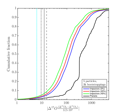
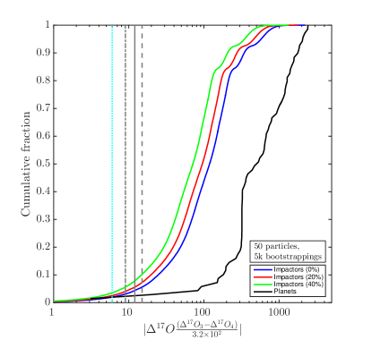
Figure 2: The same as in Figure 1, but for the bootstrapped simulations. The cumulative distributions of $\Delta^{17}O$ are shown for Earth and Theia analogs composed by at least 5 particles and $3000$ bootstrapped samples (left panel) and for a threshold of 50 particles and $5000$ bootstrapped samples (right panel).

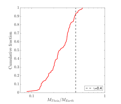
Figure 3: The final mass ratio between each Theia analog and the relative Earth analog ($\gamma$, red solid line). The vertical grey line represents the $\gamma=0.4$ threshold.

Table 1: The mean fraction (and relative $1\sigma$ Poissonian error) of compatible Earth-Theia analogs is given for different minimum numbers of particles composing the analogs ($N_{\text{min}})$, for different limits on the observed $\Delta^{17}O$ (6, 9, 12 and 15ppm) and mixing fractions (0%, 20%, 40%). $N_{\text{cases}}$ is the number of simulations with proper analogs. Results obtained imposing an upper limit of $2$ au on the semi-major axis of Mars’ analogs are reported in brackets (see Appendix A for more information).

$N_{\text{min}}$	$\Delta^{17}O$	$0$%		2$0$%		4$0$%		$N_{\text{cases}}$
	ppm	Mean (%)	$\pm\sigma$ (%)	Mean (%)	$\pm\sigma$(%)	Mean (%)	$\pm\sigma$(%)
0	6	$0$	$0$	$0$	$0$	$2.7(1.4)$	$1.9(1.4)$	75 (70)
	9	$1.3(1.4)$	$1.3(1.4)$	$2.7(1.4)$	$1.9(1.4)$	$4.0(2.9)$	$2.3(2.0)$
	12	$2.7(1.4)$	$1.9(1.4)$	$4.0(2.9)$	$2.3(2.0)$	$10.7(10.0)$	$3.8(3.8)$
	15	$4.0(2.9)$	$2.3(2.0)$	$8.0(7.1)$	$3.3(3.2)$	$10.7(10)$	$3.8(3.8)$
10	6	$0$	$0$	$0$	$0$	$2.8(1.5)$	$2.0(1.5)$	72 (67)
	9	$1.4(1.5)$	$1.4(1.5)$	$2.7(1.5)$	$1.9(1.5)$	$4.1(3.0)$	$2.4(2.1)$
	12	$2.8(1.5)$	$2.0(1.5)$	$4.2(2.9)$	$2.4(2.1)$	$11.1(10.4)$	$3.9(3.9)$
	15	$4.2(3.0)$	$2.4(2.1)$	$8.3(7.5)$	$3.4(3.3)$	$11.1(10.4)$	$3.9(3.9)$
20	6	$0$	$0$	$0$	$0$	$1.8(0)$	$1.8(0)$	55 (50)
	9	$0$	$0$	$1.8$	$1.8$	$3.6(2.0)$	$2.6(2.0)$
	12	$1.8(0)$	$1.8(0)$	$3.6(2.0)$	$2.6(2.0)$	$7.3(6.0)$	$3.6(3.5)$
	15	$3.6(2.0)$	$2.6(2.0)$	$7.3(6.0)$	$3.6(3.5)$	$7.3(6.0)$	$3.6(3.5)$
30	6	$0$	$0$	$0$	$0$	$0(3.1)$	$0(3.1)$	35 (32)
	9	$0$	$0$	$0$	$0$	$2.9(3.1)$	$2.9(3.1)$
	12	$0$	$0$	$2.9(3.1)$	$2.9(3.1)$	$8.6(9.4)$	$4.9(5.4)$
	15	$2.9(3.1)$	$2.9(3.1)$	$8.6(9.3)$	$4.9(5.4)$	$8.6(9.4)$	$4.9(6.7)$
40	6	$0$	$0$	$0$	$0$	$0$	$0$	22 (21)
	9	$0$	$0$	$0$	$0$	$0$	$0$
	12	$0$	$0$	$0$	$0$	$7.7(9.5)$	$5.4(5.4)$
	15	$0$	$0$	$9.1(11.8)$	$6.4(8.3)$	$9.1(11.8)$	$6.4(8.3)$
50	6	$0$	$0$	$0$	$0$	$0$	$0$	13 (12)
	9	$0$	$0$	$0$	$0$	$0$	$0$
	12	$0$	$0$	$0$	$0$	$7.7(8.3)$	$7.7(8.3)$
	15	$0$	$0$	$7.7(8.3)$	$7.7(8.3)$	$7.7(8.3)$	$7.7(8.3)$

To further explore and quantify the error due to granularity we used a bootstrap technique with replacement. We took the original distribution of the initial semi-major axis of the planetesimals composing each Earth, Mars and Theia analog and we extracted a new, equally populated, distribution of semi-major axis from it (see also Kaib & Cowan, 2015b). Only systems which analogs are composed of more than 5 particles ($73$ simulations) have been taken into consideration. We repeated the bootstrapping 5000 times for each distribution when the set of possible bootstrap samples was rich enough (i.e. more than minimum 10 particles, while we bootstrapped only 3000 times for bodies formed by at least 5 particles).
The Poissonian error on the fractions has been evaluated in a similar way as done in the case of the raw simulations. We show here an example of the error calculation, in which we assume that we have N simulations among which two give non null fractions, $f_{1}$ and $f_{2}$, in their bootstrapped sample. In this case, the total fraction obtained considering all the simulations is given by the sum of the probabilities of the possible outcomes

$$P=P2+P1=[2f_{1}f_{2}+f_{1}(1-f_{2})+f_{2}(1-f_{1})]/N=(f_{1}+f_{2})/N$$ (2)

The total error can be evaluated applying the error propagation on Equation 2 and assuming $\sigma(P1)=\sqrt{1}[f_{1}(1-f_{2})+f_{2}(1-f_{1})]$ and $\sigma(P2)=\sqrt{2}f_{1}f_{2}$. We evaluated the Poissonian error following a generalised version of this method, and taking into account only the bootstrapped samples that result in a non negligible fraction $f_{i}$.

3 Results

Table 2: The same as in Table 1 but for systems with minimum $5$ ($73$ simulations) or $50$ ($13$ simulations) particles composing each analog and respectively 3000 or 5000 bootstrappings. Results obtained imposing an upper limit of $2$ au on the semi-major axis of Mars’ analogs are reported in brackets (see Appendix A for more information).

$\Delta^{17}O$	$N_{\text{min}}$, $N_{\text{bss}}$	$0$%		2$0$%		4$0$%
ppm		Mean (%)	$\pm\sigma$ (%)	Mean (%)	$\pm\sigma$(%)	Mean (%)	$\pm\sigma$(%)
$6$	$5$, $3$k	$1.9(1.6)$	$1.4(1.2)$	$2.4(2.0)$	$1.6(1.4)$	$3.2(2.8)$	$2.0(1.8)$
	$50$, $5$k	$2.0(2.2)$	$1.9(1.9)$	$2.6(2.8)$	$2.4(2.5)$	$3.5(3.8)$	$3.2(3.4)$
$9$	$5$, $3$k	$2.9(2.5)$	$1.8(1.6)$	$3.6(3.2)$	$2.1(2.0)$	$4.9(4.4)$	$2.5(2.4)$
	$50$, $5$k	$3.1(3.4)$	$2.9(3.1)$	$4.0(4.4)$	$3.7(3.9)$	$5.6(6.1)$	$4.9(5.3)$
12	$5$, $3$k	$3.9(3.4)$	$2.2(2.1)$	$4.9(4.4)$	$2.5(2.4)$	$6.8(6.1)$	$3.0(2.9)$
	$50$, $5$k	$4.4(4.7)$	$3.9(4.2)$	$5.6(6.1)$	$4.9(5.3)$	$7.8(8.5)$	$6.5(7.0)$
15	$5$, $3$k	$4.9(4.4)$	$2.5(2.4)$	$6.3(5.6)$	$2.9(2.8)$	$8.8(8.0)$	$3.4(3.4)$
	$50$, $5$k	$5.6(6.1)$	$4.9(5.3)$	$7.3(7.9)$	$6.1(6.6)$	$10.2(11.0)$	$8.0(8.6)$

3.1 The composition of the Moon

When adopting an upper limit of $15$ppm for the composition difference, we find the probability of having an impact between an Earth and a Theia analog with similar oxygen isotope composition to be between 4% and 10.7%, depending on the percentage of mixing allowed (from 0% to 40%). When considering the Poissonian $1\sigma$ error the probability is $<14.5$%. Another study (Young et al., 2016) recently suggested a smaller difference of at most $6$ppm. When taking this maximal difference for oxygen composition we get 0%-2.7% probability of compatibility. Including the Poissonian error the same probability is between 0% and 4.6%. These percentages change when considering thresholds for the minimum number of bodies in each analog (see Figures 1 and Table 1).

Our results are also affected by observational errors that can be taken into account comparing the composition of the simulated systems to the lower limit, mean and upper limit of the corresponding observed quantity. Table 1 shows the fractions of compatible planet-impactor systems depending on the given constraint on the observed Earth-Moon $\Delta^{17}O$ difference.

Figure 2 shows the cumulative distribution of the differences for a minimum of 5 particles composing each body and 3000 bootstrapped combinations (left panel) for a threshold of 50 particles contributing to analog and 5000 combinations (right panel). Bootstrapping 3000 times on all the systems formed by at least 5 particles, allowing for mixing and considering the $1\sigma$ error, the probability of compatibility is smaller than 12.2% (5.2% for $6$ppm). Adopting a threshold of 50 particles and bootstrapping 5000 times on each distribution the probability is 5.6%-18.2% (2%-6.7% for $6$ppm). The fractions obtained for different thresholds, number of bootstrappings and observational constraints are listed in Table 2. All the results slightly vary (without a clear trend) when setting an upper limit ($2$ au) for Mars’ analogs semi-major axis (see Table 1, Appendix A and Figures 8 and 9 for more details.) Both Figure 1 and 2 (as well as Figures 8 and 9) show that the Earth-Theia analog couples are sistematically more similar in compositions compared to the other planets. Among all the initial configurations used in the simulations the ones with Jupiter and Saturn on eccentric orbits, in particular ejsII, produce more compatible Earth-Theia couples. The configuration with slightly eccentric orbits for Jupiter and Saturn (cjsecc) is the second most productive. Set II produces a larger fraction of positive cases than set I.

It was shown that more mass can be extracted from the proto-Earth and mix into the Moon following the impact, if the impactor mass is comparable to that of the proto-Earth (Canup, 2012). In order to get about a half of the material in the proto-lunar disk coming from the proto-Earth, the mass ratio between Theia and the Earth ($\gamma$) must be larger than $0.4$ (see Canup, 2012).
We evaluated the cumulative distribution of the mass ratios for all the simulations with proper analogs (see Figure 3) and out of 75 simulations with analogs, only 5 have $\gamma>0.4$. This corresponds to a 6.7 % (6.5% when considering an upper limit for Mars’ semi-major axis) probability that such an event could happen. Even if this probability is comparable to the one obtained for similar composition impacts, the process is efficient only when the impact involves extremely high angular momentum for the Earth-Moon system. As shown by Rufu et al. (2017), this condition is not easily attained, because of angular momentum drain during the impact. Moreover, the high angular momentum needs to be dissipated later on, which requires evection resonance due to the Sun to work efficiently (Ćuk & Stewart, 2012).

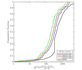
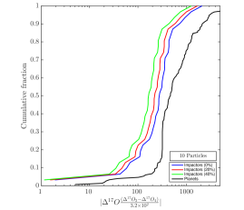
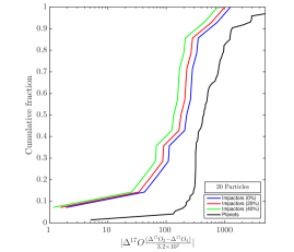
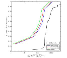
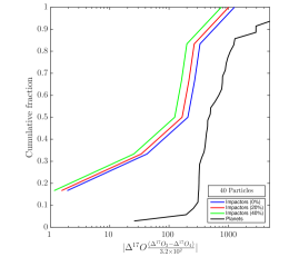
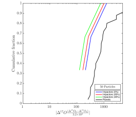
Figure 4: The same as Figure 1 but for Mars’ and its last impactor analogs. Recent SPH simulation (see Citron et al., 2015, and private communication) showed that large mixing fractions are possible. The contribution of the impactor can be up to 70% of the total mass of the proto-lunar disk from which Phobos and Deimos form. However, to be conservative, we adopted the same percentages used for the Earth-Moon system. The difference between planets and planet-impactor couples increases with the mixing fraction.

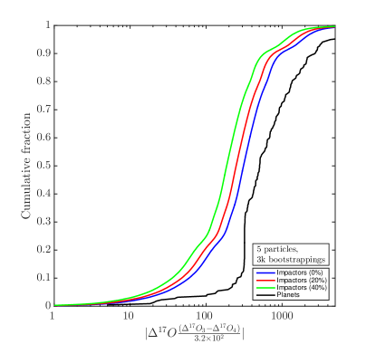
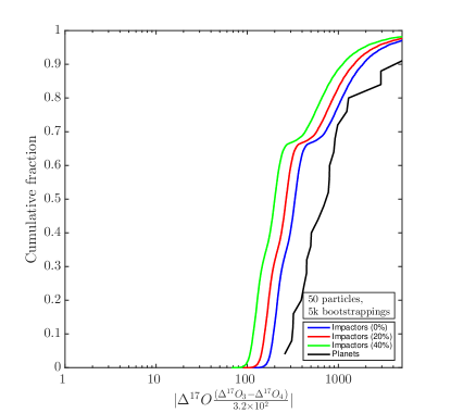
Figure 5: The same as Figure 2 but for Mars’ and its last impactor analogs.

3.2 The composition of Mars’ moons

Mars’ moons were thought to be two captured asteroids, as indicated by their morphology and composition (Murchie et al., 1991; Burns, 1978). However, recent observations (e.g., Giuranna et al., 2011; Witasse et al., 2014) showed that their composition and density is hardy reconcilable with this scenario and could be better understood if Phobos and Deimos were the result of a giant impact with a body of mass a hundred times smaller than the mass of their target (Craddock, 2011; Citron et al., 2015).

We evaluated the cumulative distribution of the $\Delta^{17}O$ between Mars and its last impactor from both the raw simulations (see Figure 4) and from the bootstrapped sample (see Figure 5).

From the comparison between Figures 4 and 5 and Figures 1 and 2 (and between Figures 10 and 11 and Figures 8 and 9) it is apparent that, if Mars’ moons are the result of a giant impact, the differences between Mars analogs and the relative last impactors are smaller than those found between the planets formed in the system, but larger than the differences found for the Earth-Theia analogs. In conclusion, we do not expect any extreme composition similarity between Phobos or Deimos and Mars, however we predict a smaller difference respect to what would be expected in case of captured asteroids.

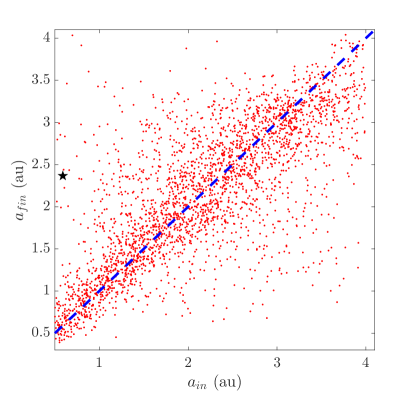
Figure 6: The planetesimals that survive without impacting any planetary embryo until the end of each simulation with proper analogs. Their final position is plotted against their initial position. Particles that did not move from their original position lay on the blue dashed line. The black star shows the position of Vesta in the diagram, if its initial semi-major axis is calculated relying on a Solar System-based calibration.

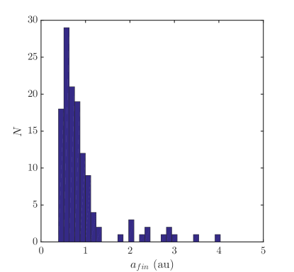
Figure 7: Histogram showing the distribution of the final semi-major axis of the asteroids initially between $0.46$ and $0.72$ au, i.e. Vesta’s initial radial range allowed by the error. Among all the asteroids, 8.7% are scattered beyond $2$ au, i.e. in the asteroid belt, by the end of the simulation.

3.3 Solar system asteroids and the composition of Vesta

Vesta is a large differentiated rocky asteroid that formed during the first few million years of the Solar System, after the formation of the first solid planetesimals (Marchi et al., 2012). Its $\Delta^{17}O$ ($-250\pm 80$, compared to $0$ppm and $320$ppm for the Earth and Mars; Clayton & Mayeda, 1996; Franchi et al., 1999) suggest this asteroid did not form in the current position. Since its isotopic composition does not match the composition gradient in the Solar System, Vesta could have formed closer to, or farther from the Sun to be then scattered on its current orbit (see Bottke et al., 2006).

To check this hypothesis we compared the initial and the final semi-major axis of the survived planetesimals in the simulations that contain proper analogs (see Figure 6). The simulated planetesimals have a mass two orders of magnitude larger than Vesta, however, they are the smallest particles followed in our simulation and so they serve as the best reference for the asteroid distribution.

Adopting the current position and compositions of the Earth and Mars to calibrate the Solar System $\Delta^{17}O$ gradient (see Eq. 1) we obtain that Vesta had an initial semi-major axis $a_{i}=0.59\pm 0.13$au (see black star in Figure 6). If we consider all the asteroids, only a small fraction of them (3%) are scattered as much as expected for Vesta. However, if we consider only the asteroids with an initial semi-major axis in the radial bin allowed for Vesta, i.e. between $0.46$au and $0.72$au, we find that 8.7% of these objects are significantly scattered in the asteroid belt, acquiring a semi-major axis larger than $2$ au by the end of the simulation (see Figure 7). The scattering process in the early stages of the Solar System could then be one of the possible explanations for the existence of outliers like Vesta, beside predicting many other similar objects.

4 Summary and Conclusions

In this paper we used a large (140) sample of simulations of rocky planets formation to compare the composition of the Earth and Theia and the composition of Mars to that of its last impactor. We also considered the case of Vesta, an asteroid whose position and composition do not match. Here we summarise the main results of this work.

• Considering all the systems, the raw simulation data yield a probability to get a moon with similar oxygen isotope composition to the Earth between 4% and 14.5% (0%-4.6% for the $6$ppm limit), depending on the percentage of mixing allowed (0 to 40%) and $1\sigma$ Poissonian error.

• The analogs of the Earth and of Theia are sistematically more similar than the planets.

• To evaluate the effect of granularity affecting our simulations, we applied a bootstrapping technique with replacement to all the simulations and we obtained new probabilities from the larger data sample obtained in this way. Including the possibility of mixing and considering the $1\sigma$ error, we find the probability of compatibility to be 4.9%-12.2% (1.9%-5.2% for $6$ppm), when taking into account only systems with analogs formed by at least 5 particles and $3000$ bootstrapped samples. When considering a threshold of 50 particles composing each analog and bootstrapping 5000 times the probability is between 5.6% and 18.2% (2%-6.7% for $6$ppm). This fraction is somewhat lower than what found in Paper I for the reasons listed above, but generally confirms our previous results, showing that the composition similarity could arise naturally from the primordial composition similarity between the proto-Earth and Theia, hence potentially alleviating the main challenge to the giant-impact scenario. Moreover, even if the probability we find is comparable to the likelihood for a high mass-ratio impact ($6.7$%) such as suggested by Canup (2012), it does not require fine-tuned condition and extremely high-spin for the proto-Earth (Ćuk & Stewart, 2012).

• Mars’ moons are expected to show a significantly different composition compared with their Mars-analog host.

• Asteroids, identified as the planetesimals that survive till the end of the simulation, can be scattered significantly far away their initial position. We found that 8.7% of our leftover planetesimals with initial semi-major axis compatible, within the error, with the one evaluated for Vesta are farther from the Vesta linear expectation of non-migrating asteroids. This process could explain the mismatch between Vesta distance from the Sun and its composition, as also predicted by Bottke et al. (2006).

We conclude that, as already found by Kaib & Cowan (2015a, b), the impact between enough similar planets is rare; however this is the most probable and less fine-tuned mechanism able to explain the formation of the Moon, its properties and composition. The giant-impact scenario, with its $\sim 10\%$ probability to lead to a Earth-Moon similar composition is currently the most consistent model available. If Mars’ moons are the result of a giant impact it is highly improbable to get to similar composition to their planet. Asteroids are not expected to closely follow the initial composition gradient in the proto-planetary disk, since they could have been scattered from their initial position. More detailed simulations are needed to further explore these issues and many other open questions related to our Solar System.

Appendix A Mars’ semi-major axis

In order to check whether our choices affect the composition gradient of the proto-planetary disk, we repeated our analysis setting an upper limit of $2$ au on the semi-major axis of Mars’ analogs. As shown in Tables 1 and 2 there is no clear trend caused by this constraint (see also Figures 8 and 9).
Figure 3 does not change significantly and therefore, we are not showing its analog here. The probability to have an impact between two bodies with $\gamma>0.4$ is slightly smaller (6.5%).
Repeating the analysis for Mars’ moons we obtained comparable results to the ones obtained without limiting Mars’ semi-major axis (see Figures 10 and 11).
Vesta has the same probability to be a scattered asteroid; Figures 6 and 7 are unchanged.

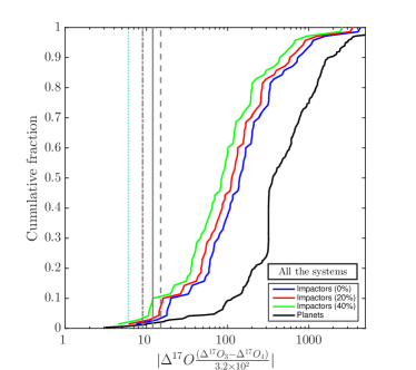
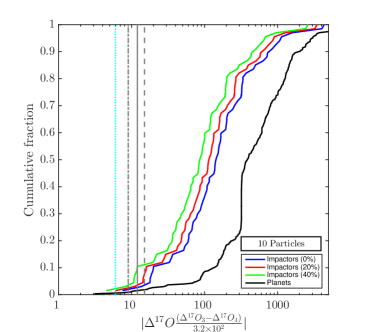
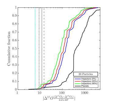
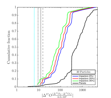
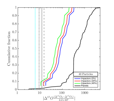
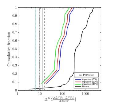
Figure 8: The same as Figure 1 obtained using an upper limit of $2$ au for the semi-major axis of Mars’s analogs.

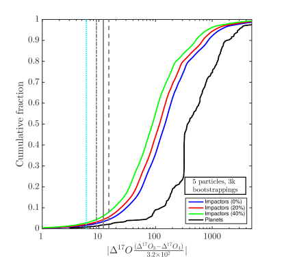
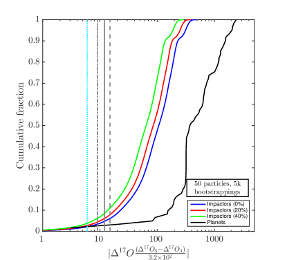
Figure 9: The same as Figure 2 obtained using an upper limit of $2$ au for the semi-major axis of Mars’s analogs.

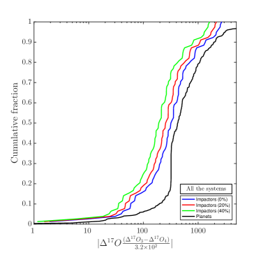
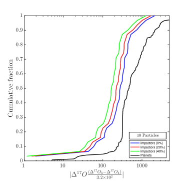
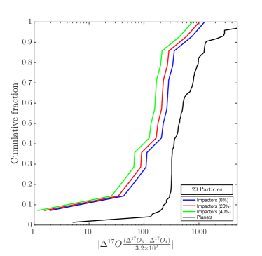
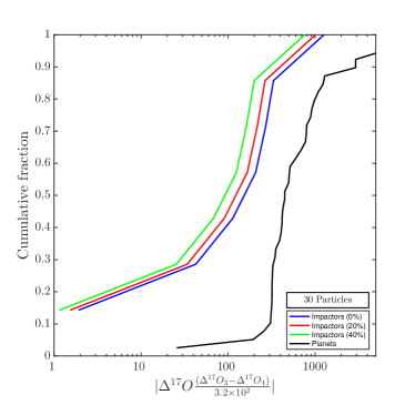
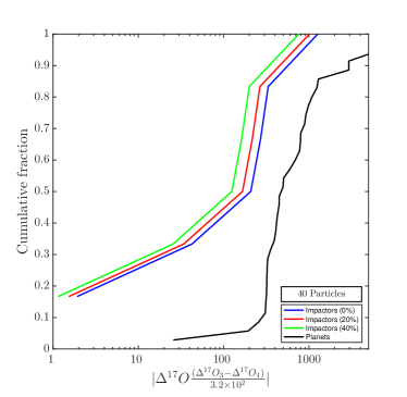
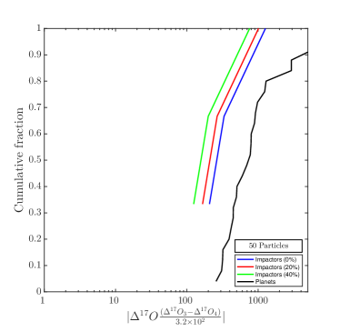
Figure 10: The same as Figure 4 obtained using an upper limit of $2$ au for the semi-major axis of Mars’s analogs.

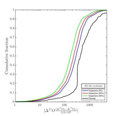
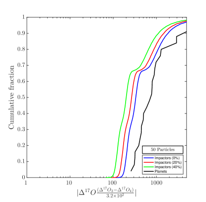
Figure 11: The same as in Figure 5 obtained using an upper limit of 2au for the semi-major axis of Mars’s analogs.

Appendix B Step-function

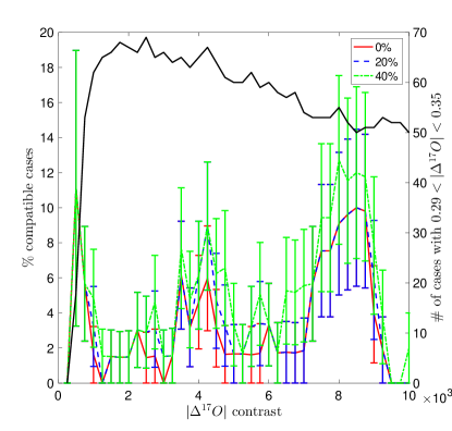
Figure 12: The $\Delta^{17}O$ difference between the Earth’s and Theia’s analogs, and the relative $1\sigma$ poissonian error, are shown as a function of the contrast between the inner and outer proto-planetary disk for mixing fractions of 0%, 20% and 40% (red solid, blue dashed and green dot dashed lines). The black solid line is the number of cases in which the composition difference between the Earth and Mars is found to be in the correct range.

The composition gradient of the proto-planetary disk is unknown; the assumption of a linear gradient done in Section 2.3 is then only one of the possible functions that can be used to model the $\Delta^{17}O$ distribution. Many functions have been used in literature (see Kaib & Cowan, 2015a; Young et al., 2016), however, according to the recent results presented by Dauphas (2017), the composition of the proto-planetary disk was not random, and the Earth and Theia aggregated mostly from planetesimals with a similar composition. Using lithophile, as well as moderately and highly siderophile elements to trace the accretion history of the Earth, Dauphas (2017) found that the inner proto-planetary disk had a homogeneous composition, dominated by enstatite chondrites, while the outer part contained a larger fraction of ordinary chondrites. Therefore, we tested the giant-impact scenario assuming a sharp contrast between the composition of inner and outer terrestrial planets modelled as a step function for the $\Delta^{17}O$ distribution. As done by Kaib & Cowan (2015a) we initially fixed a $\Delta^{17}O$ contrast and then evaluated the heliocentric distance at which the change has to occur in order to have a $\Delta^{17}O$ between Mars and the Earth of $320\pm 30$ppm. We used contrasts between 0 and $10^{4}$ppm (Kaib & Cowan, 2015a; Burbine & O’Brien, 2004; Ozima et al., 2007) and we evaluated the fraction of compatible Earth-Theia couples in each case. We assumed an upper limit of $2$ au for Mars’ analogs semi-major axis. The number of cases for which it is possible to approximately reproduce the composition difference between Mars and the Earth (black solid line in Figure 12) peaks around a contrast of $2000$-$4000$ppm and produces 50-70 cases for larger contrasts. The fraction of positive cases varies significantly with the contrast and the fraction of mixing, ranging between 0% and 19% when considering the 1$\sigma$ Poissonian error. Therefore, using a step function for the composition gradient can produce a significant number of compatible impacts, comparable to what obtained when adopting a linear distribution.

References

- Agnor et al. (1999) Agnor C. B., Canup R. M., Levison H. F., 1999, Icarus, 142, 219
- Bottke et al. (2006) Bottke W. F., Nesvorný D., Grimm R. E., Morbidelli A., O’Brien D. P., 2006, Nature, 439, 821
- Bromley & Kenyon (2017) Bromley B. C., Kenyon S. J., 2017, preprint, (arXiv:1703.10618)
- Burbine & O’Brien (2004) Burbine T. H., O’Brien K. M., 2004, Meteoritics and Planetary Science, 39, 667
- Burns (1978) Burns J. A., 1978, Vistas in Astronomy, 22, 193
- Canup (2012) Canup R. M., 2012, Science, 338, 1052
- Canup & Asphaug (2001) Canup R. M., Asphaug E., 2001, Nature, 412, 708
- Chambers (1999) Chambers J. E., 1999, MNRAS, 304, 793
- Citron et al. (2015) Citron R. I., Genda H., Ida S., 2015, Icarus, 252, 334
- Clayton & Mayeda (1996) Clayton R. N., Mayeda T. K., 1996, Geochimica et Cosmochimica Acta, 60, 1999
- Craddock (2011) Craddock R. A., 2011, Icarus, 211, 1150
- Ćuk & Stewart (2012) Ćuk M., Stewart S. T., 2012, Science, 338, 1047
- D’Angelo & Marzari (2012) D’Angelo G., Marzari F., 2012, ApJ, 757, 50
- Dauphas (2017) Dauphas N., 2017, Nature, 541, 521
- Franchi et al. (1999) Franchi I. A., Wright I. P., Sexton A. S., Pillinger C. T., 1999, Meteoritics and Planetary Science, 34, 657
- Giuranna et al. (2011) Giuranna M., Roush T. L., Duxbury T., Hogan R. C., Carli C., Geminale A., Formisano V., 2011, PLANSS, 59, 1308
- Herwartz et al. (2014) Herwartz D., Pack A., Friedrichs B., Bischoff A., 2014, Science, 344, 1146
- Jacobsen (2005) Jacobsen S. B., 2005, Annual Review of Earth and Planetary Sciences, 33, 531
- Jacobson & Morbidelli (2014) Jacobson S. A., Morbidelli A., 2014, Royal Society of London Philosophical Transactions Series A, 372, 174
- Kaib & Cowan (2015a) Kaib N. A., Cowan N. B., 2015a, Icarus, 252, 161
- Kaib & Cowan (2015b) Kaib N. A., Cowan N. B., 2015b, Icarus, 258, 14
- Lugmair & Shukolyukov (1998) Lugmair G. W., Shukolyukov A., 1998, Geochimica et Cosmochimica Acta, 62, 2863
- Marchi et al. (2012) Marchi S., et al., 2012, Science, 336, 690
- Mastrobuono-Battisti et al. (2015) Mastrobuono-Battisti A., Perets H. B., Raymond S. N., 2015, Nature, 520, 212
- Murchie et al. (1991) Murchie S. L., et al., 1991, JGR, 96, 5925
- Ozima et al. (2007) Ozima M., Podosek F. A., Higuchi T., Yin Q.-Z., Yamada A., 2007, Icarus, 186, 562
- Pahlevan & Stevenson (2007) Pahlevan K., Stevenson D. J., 2007, Earth and Planetary Science Letters, 262, 438
- Raymond et al. (2009) Raymond S. N., O’Brien D. P., Morbidelli A., Kaib N. A., 2009, Icarus, 203, 644
- Raymond et al. (2013) Raymond S. N., Kokubo E., Morbidelli A., Morishima R., Walsh K. J., 2013, Protostars and Planets VI, University of Arizona Press (2014), eds. H. Beuther, R. Klessen, C. Dullemond, Th. Henning.,
- Ringwood (1986) Ringwood A. E., 1986, Nature, 322, 323
- Rufu et al. (2017) Rufu R., Aharonson O., Perets H. B., 2017, Nature Geoscience, 10, 89
- Touboul et al. (2007) Touboul M., Kleine T., Bourdon B., Palme H., Wieler R., 2007, Nature, 450, 1206
- Walsh et al. (2011) Walsh K. J., Morbidelli A., Raymond S. N., O’Brien D. P., Mandell A. M., 2011, Nature, 475, 206
- Wang & Jacobsen (2016) Wang K., Jacobsen S. B., 2016, Nature, advance online publication,
- Wiechert et al. (2001) Wiechert U., Halliday A. N., Lee D.-C., Snyder G. A., Taylor L. A., Rumble D., 2001, Science, 294, 345
- Witasse et al. (2014) Witasse O., Duxbury T., Chicarro A., et al., 2014, PLANSS, 102, 18
- Young et al. (2016) Young E. D., Kohl I. E., Warren P. H., Rubie D. C., Jacobson S. A., Morbidelli A., 2016, Science, 351, 493
- Zhang et al. (2012) Zhang J., Dauphas N., Davis A. M., Leya I., Fedkin A., 2012, Nature Geoscience, 5, 251