The COM-negative binomial distribution: modeling overdispersion and ultrahigh zero-inflated count data
Abstract
In this paper, we focus on the COM-type negative binomial distribution with three parameters, which belongs to COM-type class distributions and family of equilibrium distributions of arbitrary birth-death process. Besides, we show abundant distributional properties such as overdispersion and underdispersion, log-concavity, log-convexity (infinite divisibility), pseudo compound Poisson, stochastic ordering and asymptotic approximation. Some characterizations including sum of equicorrelated geometrically distributed random variables, conditional distribution, limit distribution of COM-negative hypergeometric distribution, and Stein’s identity are given for theoretical properties. COM-negative binomial distribution was applied to overdispersion and ultrahigh zero-inflated data sets. With the aid of ratio regression, we employ maximum likelihood method to estimate the parameters and the goodness-of-fit are evaluated by the discrete Kolmogorov-Smirnov test.
keywords:
overdispersion , zero-inflated data , infinite divisibility , Stein’s characterization , discrete Kolmogorov-Smirnov test MSC2010: 60E07 60A05 62F101 Introduction
Before 2005, Conway-Maxwell-Poisson distribution (denoted as COM-Poisson distribution) had been rarely used since Conway and Maxwell (1962) briefly introduced it for modeling of queuing systems with state-dependent service time, see also Wimmer and Altmann (1999), Wimmer et al. (1995). About ten years ago, the COM-Poisson distribution with two parameters was revived by Shmueli et al. (2005) as a generalization of Poisson distribution. More recently, there has been a fast growth of researches on COM-Poisson distribution in terms of related statistical theory and applied methodology, see Sellers et al. (2012) and the references therein. The probability mass function (p.m.f.) of the COM-Poisson random variable (r. v) is given by
| (1) |
where and . We denote (1) as .
Kokonendji et al. (2008) proved that COM-Poisson distribution was overdispersed when and underdispersed when . Another extension of Poisson is negative binomial, which is a noted discrete distribution with overdispersion property and is widely applied in actuarial sciences(see Denuit et al. (2007), Kaas (2008)). The p.m.f. of the negative binomial r.v is
| (2) |
where and .
In this paper, we propose a COM-negative binomial (denoted by CMNB) distribution , which extends the negative binomial distribution and depends on three parameters by replacing in (2) with and divide the normalization constant .
Definition 1.1.
A r.v. is said to follow CMNB distribution with three parameters if the p.m.f. is given by
| (3) |
where and .
When , we will show that CMNB (3) is discrete compound Poisson, which has wide application in risk theory (includes non-life insurance) as well, see Zhang et al. (2014) and the references therein. For illustrating the p.m.f of defined in (3), we plot 12 cases of CMNB in Figture 1.
It is easy to see that our CMNB distribution belongs to the COM-type extension of class. The class distribution is a famous family of distributions which sometimes refers to Katz class (see remarks in section 2.3.1 of Johnson et al. (2005)). It has significant applications in non-life insurance mathematics, especially for modelling claim counts ( loss models, collective risk models), see Denuit et al. (2007). A classic result in non-life insurance textbooks states that the class distribution only contains degenerate, binomial, Poisson and the negative binomial distribution. After adding a new parameter , we define the COM-type extension of distribution, and it is convenient to see that degenerate, COM-Poisson, COM-binomial and CMNB belong to this class of distributions.
Shmueli et al. (2005) firstly proposed the COM-binomial distribution which is presented as a sum of equicorrelated Bernoulli variables. Borges et al. (2014) studied some properties and an asymptotic approximation (e.g. COM-binomial approximates to COM-Poisson under some conditions) of this family of distributions in detail. We will show that some results of COM-Poisson can be extended in our CMNB distribution. Kadane (2016) gave the exchangeably properties, sufficient statistics and multivariate extension of COM-binomial distribution. Another variant of CMNB distribution has been studied by Imoto (2014), it just replaced the term in (2) by and then divided the normalization constant. We will give adequate reasons to support our extension in succeeding sections. Chakraborty and Imoto (2016) considered the extended COM-Poisson distribution (ECOMP):
| (5) |
where the parameter space is . ECOMP distribution combines Imoto (2014)’s extension (), Chakraborty and Ong (2016)’s extension (COMNB with ) and the CMNB distribution (3) with . The COM-Poisson is a special case of ECOMP when . ECOMP distribution (5) has the queuing systems characterization (birth-death process with arrival rate and service rate for ), see also Brown and Xia (2001) for arbitrary birth-death process characterization.
The rest of the article is organized as the follows. In section 2, we propose the COM-type class distributions and demonstrate some example of COM-type class which includes the CMNB. Further more, some properties of CMNB, such as Renyi entropy and Tsallis entropy representation, overdispersion and underdispersion, log-concavity, log-convexity (infinite divisibility), pseudo compound Poisson, stochastic ordering and asymptotic approximation are studied. In section 3, some conditional distribution characterizations and Stein identity characterization are presented by using related lemmas, and we also show that COM-negative hypergeometric can approximate to CMNB. In section 4, inverse methods were introduced to generate CMNB distributed random variables. Section 5 then estimates the parameters by maximum likelihood method, in which the initial values are provided by recursive formula. In section 6, two simulated data sets and two applications to actuarial claim data sets are given as examples. In section 7, we provide some potential and further research suggestions based on the properties and characterizations of CMNB distribution.

2 Properties
2.1 Recursive formula and ultrahigh zero-inflated property
The recursive formula (or ratios of consecutive probabilities) is given by
| (6) |
We say that a zero-inflated count data following some discrete distribution is ultrahigh zero-inflated if . For CMNB case with two parameters, we have ; and for negative binomial case, we get If we choose and in CMNB case, then this CMNB distribution is more flexible to deal with the ratio comparing to the NB distribution, as when . (For examples, the plots of CMNB distribution with in Figure 1; in Table 4 of section 6.2). In the insurance company, the more zero insurance claims, the less risk to bankrupt. The following definition provides a generalization of class distribution.
Definition 2.1.
Let be a discrete r.v., if satisfies the recursive formula
| (7) |
for some constants and , then we call it COM-type class distribution. We denote this class as .
The COM-Poisson distribution satisfies the case , since and .
From (6), it is easy to see that CMNB distribution belongs to COM-type class distribution with .
| (8) |
The COM-binomial distribution (CMB), see Shmueli et al. (2005), Borges et al. (2014), with p.m.f.
| (9) |
where . We denote (9) as . Since the ratio of consecutive probabilities is , COM-binomial distribution belongs to COM type class distribution.
Remark 1: As we know, the class distribution only contains degenerate distribution, binomial distribution, Poisson distribution and the negative binomial distribution. But there are other distributions belongs to COM type class. For example, can be replaced by in (9), and the p.m.f. is given by
where such that .
Remark 2: Brown and Xia (2001) considered the very large class of stationary distribution of birth-death process with arrival rate and service rate by the recursive formula:
Thus we can construct a birth-death process with arrival rate and service rate , and is a positive constant, which characterizes the COM-type class distribution.
2.2 Related to Rényi entropy and Tsallis entropy
Notice the Rényi entropy (see Rényi (1961)) in the information theory, which generalizes the Shannon entropy. The Renyi entropy of order of a discrete r.v. :
Let be negative binomial distributed in (2) and be CMNB distributed in (4). Then the normalization constant in (4) has Rényi entropy representation , so .
Another generalization of Shannon entropy in physic is the Tsallis entropy. For r.v. , its Tsallis entropy of order is defined by
This entropy was introduced by Tsallis (1988) as a basis for generalizing the Boltzmann-Gibbs statistics. Also, the normalization constant in (4) has Tsallis entropy representation , then .
2.3 Log-concave, Log-convex, Infinite divisibility
This subsection deals with log-concavity and log-convexity of the CMNB distribution. A discrete distribution with is said to have log-concave (log-convex) p.m.f. if
Lemma 2.1.
The CMNB distribution is log-concave if and log-convex if .
Proof.
In fact, using the ratio of consecutive probabilities (6), we have
Then iff (log-concave) and iff (log-convex). ∎
Remark 3: Ibragimov (1956) called a distribution strongly unimodal if it is unimodal and its convolution with any unimodal distribution is unimodal. He showed that the strongly unimodal distributions is equivalent to the log-concave distributions. So CMNB distribution has strong unimodality(see Figure 1 for example) when . Steutel (1970) showed that all log-convex discrete distributions are infinitely divisible, the background and detailed proof can be found in Steutel and van Harn (2003). Then we obtain infinite divisibility of CMNB distribution when .
Corollary 2.1.
The CMNB distribution (3) is discrete infinitely divisible (discrete compound Poisson distribution) if .
Feller’s characterization of the discrete infinite divisibility showed that a non-negative integer valued r.v. is infinitely divisibleiff its distribution is a discrete compound Poisson distribution with probability generating function (in short, p.g.f.):
| (10) |
where
For a theoretical treatment of discrete infinite divisibility (or discrete compound Poisson distribution), we refer readers to section 2 of Steutel and van Harn (2003), section 9.3 of Johnson et al. (2005), Zhang and Li (2016).
Considering some being negative in (10), it turns into a generalization of the discrete compound Poisson distribution:
Definition 2.2 (Discrete pseudo compound Poisson distribution).
If a discrete r.v. with , , has a p.g.f. of the form
| (11) |
where , , , and , then is said to follow a discrete pseudo compound Poisson distribution, abbreviated as DPCP.
Next, we will give two lemmas on the non-vanishing p.g.f. characterization of DPCP, see Zhang et al. (2014) and Zhang et al. (2017).
Lemma 2.2.
Let , for any discrete r.v. , its p.g.f. has no zeros in iff is DPCP distributed.
The proof of Lemma 2.2 is based on Wiener-Lévy theorem, which is a sophisticated theorem in Fourier analysis, see Zygmund (2002).
Lemma 2.3.
(Lévy-Wiener theorem) Let be a absolutely convergent Fourier series with . The value of lies on a curve , and is an analytic (not necessarily single-valued) function of a complex variable which is regular at every point of . Then has an absolutely convergent Fourier series.
Lemma 2.4.
For any discrete r.v. with p.g.f. . If , then is DPCP distributed.
Proof.
First, we show that has no zeros in , since
And notice that , so are not zeros point. ∎
The condition in the next corollary is weaker than that of Corollary 2.1, and the result (DPCP) is also weaker than Corollary 2.1 (DCP).
Corollary 2.2.
The CMNB distribution (3) is discrete pseudo compound Poisson distribution if or .
Proof.
On the one hand, deduces that CMNB belongs to discrete compound Poisson by Corollary 2.1, hence CMNB is discrete pseudo compound Poisson. On the other hand, by using Lemma 2.4, we need to guarantee that for . The is a decreasing function with respect to when , reaches its maximum as . So is the other case. ∎
Applying the recurrence relation (Lévy-Adelson-Panjer recursion) of p.m.f. of DPCP distribution, see Remark 1 in Zhang et al. (2014)
and , then the DPCP parametrization of CMNB is determined by the following system of equations:
where .
2.4 Overdispersion and underdispersion
In statistics, for a given random sample , overdispersion means that . Conversely, underdispersion means that . Moreover, equal-dispersion means that . Gómez-Déniz (2011) summerized the phenomena of insurance count claims data, which were characterized by two features: (i) Overdispersion, i.e., the variance is greater than the mean; (ii) Zero-inflated, i.e. the presence of a high percentage of zero values in the empirical distribution.
The CMNB distribution belongs to the family of weighted Poisson distribution (see Kokonendji et al. (2008)) with p.m.f.
| (12) |
where is a non-negative weighted function.
Then weighted Poisson representation of CMNB distribution is
Therefore, CMNB distribution in (3) can be seen as a weighted Poisson distribution with weighted function
| (13) |
Theorem 3 and its corollary in Kokonendji et al. (2008) provide an “iff” condition to prove overdispersion and underdispersion of the weighted Poisson distribution.
Lemma 2.5.
Let be a weighted Poisson random variable with mean , and let be a weighted function not depending on . Then, weighted function is logconvex (logconcave) iff the weighted version of is overdispersed (underdispersed).
Kokonendji et al. (2008) applied it to show that COM-Poisson distribution is overdispersion if and underdispersion if . We employ their methods to get a criterion for overdispersion or underdispersion of CMNB distribution.
Theorem 2.1.
Set . The COM-nagative binomial distribution (3) is overdispersion if and underdispersion if .
Proof.
Then, the results of overdispersion can be easily obtained by Theorem 2.1.
Corollary 2.3.
In these two cases: 1. ; 2. . CMNB distribution is overdispersion.
Remark 4: The result of case 2 () can be also obtained from Corollary 2.1 and overdispersion of discrete compound Poisson distribution (equivalently, the discrete infinitely divisible).
2.5 Stochastic ordering
Stochastic ordering is the concept of one r.v. neither stochastically greater than, less than nor equal to another r.v. . There are plenty types of stochastic orders, which have various applications in risk theory. Firstly, we present 4 different definitions for discrete r.v.: usual stochastic order, likelihood ratio order, hazard rate order and mean residual life order.
1. is stochastically less than in usual stochastic order (denoted by ) if for all , where is the survival function of with p.m.f. .
2. is stochastically less than in likelihood ratio order (denoted by ) if increases in over the union of the supports of and , where and denotes the p.m.f. of and , respectively.
3. is stochastically less than in hazard rate order (denoted by ) if for all , where the hazard function of a discrete r.v. with p.m.f. is defined as .
4. is stochastically less than in mean residual life order (denoted by ) if for all , where the mean residual life function of a discrete r.v. with p.m.f. is defined as .
The relationship among the above four stochastic ordering are
(see Theorem 1.C.1 of Shaked and Shanthikumar (2007)) and (see Theorem 1.B.1 of Shaked and Shanthikumar (2007)).
Gupta et al. (2014) gave the stochastic ordering between COM-Poisson r.v. and Poisson distributed r.v. with same parameter in (1), that is , therefore , and . In the following result we will show that CMNB distribution also has some stochastic ordering properties.
Theorem 2.2.
Let and be two r.vs following CMNB distribution with parameters and , respectively. If , then , hence , and .
Proof.
Note that , we have . Then
which is increasing in as . ∎
Especially, assume that is a positive integer, the CMNB should be called the COM-Pascal distribution. Let be CMNB distributed and be negative binomial distributed with the same parameters , it yields to when .
The next theorem is proved in the view of weighted Poisson distribution (12) from weighted function of CMNB distribution. Example 1.C.59 of Shaked and Shanthikumar (2007) states the obvious lemma below:
Lemma 2.6.
Define as the r.v. with weighted density function , Similarly, for another nonnegative r.v. with density function , define as the r.v. with the weighted density function . If is an increasing function, then .
Theorem 2.3.
Let and be two CMNB distributed with parameters and , respectively. If or , then , and therefore , and
Proof.
For Poisson distributed , with mean ,, if , then is increasing for all . So . From section 2.4, we know that CMNB is weight Poisson with weight (13).
On the one hand, when , we notice that weighted density function for CMNB distribution is increasing with respect to . On the other hand, is an increasing function with respect to as , that is, . ∎
2.6 Approximate to COM-Poisson distribution
The next theorem enables CMNB distribution to be a suitable generalization since its limit distribution is the COM-Poisson under some conditions. We prove that CMNB distribution converges to the COM-Poisson distribution when goes to infinity.
Theorem 2.4.
Suppose that r.v. has CMNB distribution with parameters , denote the p.m.f. as , and let . Then
| (14) |
Proof.
3 Characterizations
3.1 Sum of equicorrelated geometrically distributed r.v.
It is well known that the binomial r.v. can be seen as the sum of independent Bernoulli r.v. .
where
Shmueli et al. (2005) and Borges et al. (2014) mentioned that the COM-binomial distribution (9) can be presented as a sum of equicorrelated Bernoulli r.vs with joint distribution
where .
As we know, negative binomial distribution can be treated as the sum of independent geometric r.vs :
where
It is similar to see that the CMNB distribution can be interpreted as a sum of equicorrelated geometric r.vs with joint distribution
| (15) |
where .
The reason is that we assume is equicorrelated, and has feasible positive integer solutions, and each solution has probability . Then, the possible values of random vector such that is CMNB distributed, namely
Thus we have (15).
3.2 Conditional distribution
In this subsection, two conditional distribution characterizations are obtained for CMNB distribution. For two independent r.vs , what is the form of the conditional distribution of given ? Consider the sum of CMNB r.vs with parameters and , then
The conditional distribution is
| (16) |
Using (16), we naturally define the p.m.f. of COM-negative hypergeometric distribution with parameter as follow:
| (17) |
where and is the normalization constant.
When , COM-negative hypergeometric distribution turns out to be negative hypergeometric distribution, see Wimmer and Altmann (1999), Johnson et al. (2005).
By Patil and Seshadri (1964)’s general characterization theorem for negative binomial, Poisson and geometric distribution, we know that, given , if the conditional distribution is negative hypergeometric with parameters and for all values of the sum ,
then and both are negative binomial distribution, with parameters and ,
respectively (see also Kagan et al. (1973)).
Lemma 3.1.
(Patil and Seshadri (1964)) Let and be independent and both discrete (or both continuous) r.vs and suppose is the function . If is of the form where is an arbitrary non-negative function, then
| (18) |
where and are the corresponding normalizer for and which make them p.m.f..
Now we apply Lemma 3.1 for characterizing CMNB distribution.
Theorem 3.1.
Let X,Y be the independent discrete r.v. with and . If the is the COM-negative hypergeometric distribution (17) with parameters for all , then both and have the CMNB distributions with the parameters and respectively.
Proof.
Rao and Rubin (1964) study the following characterization of the Poisson distribution: If is a discrete r.v. taking only nonnegative integer values and the conditional distribution of given is binomial distribution with parameters ( does not depend on ), then follows the Poisson distribution iff
Based on the COM-negative hypergeometric distribution above and an extension of Rao and Rubin (1964)’s characterization which established by Shanbhag (1977), the Rao-Rubin characterization for CMNB is obtained.
Lemma 3.2.
Next, we give the following CMNB extension of Rao-Rubin characterization. The Shanbhag’s result is vital to prove this extension immediately.
Theorem 3.2.
Let be the non-negative integer-valued r.vs such that with , and
then iff follows the CMNB distribution with the parameters for some .
3.3 COM-negative hypergeometric approximate to CMNB
We have shown that the conditional distribution of CMNB r.v. given the sum of two CMNB random variables and follows the COM-negative hypergeometric distribution (17). Next, we show that the COM-negative hypergeometric distribution (17) converges to the CMNB distribution (3).
Theorem 3.3.
Let be the COM-negative hypergeometric r.v. with parameters and p.m.f. given by (17), Assume , , , then
Proof.
First, we multiply the p.m.f of COM-negative hypergeometric distribution by the normalization constant (see (17)):
Using the Stirling’s formula for the Gamma function, , it yields
From the conditions, we have as . Then
and
Finally, we obtain
Note that the normalizing constant exsists and does not depend on . Therefore, is the p.m.f. of via comparing with (3). ∎
Borges et al. (2014) showed that the COM-Poisson distribution is the limiting distribution of the COM-binomial distribution. Let (see (9)) and for , then
namely .
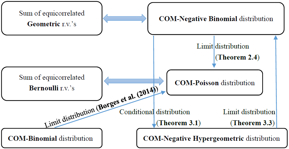
To sum up, judging from the above mentioned theorems of limiting distribution, we may naturally draw the relationships among some COM-type distributions in Figure 2.
3.4 Functional operator characterization by Stein’s identity
Using recursive formula (6) for CMNB distribution, an extension of functional operator characterization which arises from the negative binomial approximation literatures by Stein-Chen method is presented. The following Stein’s lemma also can be derived from the work of Brown and Xia (2001) who give a large class of approximation distribution which is the equilibrium distribution of a birth-death process with arbitrary arrival rate and service rate.
The functional operator characterization is well-known in the Stein-Chen method literatures. Lemma 3.3 extends the Lemma 1 in Brown and Phillips (1999) for negative binomial approximation.
Lemma 3.3.
The r.v. has distribution iff the equation
| (19) |
holds for any bounded function .
4 Generating CMNB-distributed random variables
The inverse transform sampling is a basic method in pseudo-random number sampling, namely for generating sample numbers at random from any probability distribution given its cumulative distribution function. The following lemmas are the basis of inverse method.
Lemma 4.1.
Suppose is the cumulative distribution function of random variable , then is uniformly distributed in interval .
Lemma 4.2.
Suppose , for any cumulative distribution function , let , then , that is, is the distribution function of random variable .
The proof of Lemma 4.1 and 4.2 is trivial and can be found in text books of computational statistics.
Consider generating random sample from CMNB, since the p.m.f. is
| (20) |
It follows easily that
| (21) |
Multiplying these equations yields
Thus, for any non-negative , the distribution function can be easily calculated. By Lemma 4.2, the inverse method alternates between the following steps:
- Step 1:
-
Let , ;
- Step 2:
-
Generate a random sample , and fix its value;
- Step 3:
-
Let ;
- Step 4:
-
If , then ; Otherwise, let , and back to Step 3;
We conclude that, is the random number drawn from the CMNB distribution with parameters .
5 Estimations
5.1 Estimation by three recursive formulas
The method of recursive formula estimation (or refer as ratio regression, see Bohning (2016)) which give crude estimations of the estimated parameters, is originated with Shmueli et al. (2005), and extended by Imoto (2014). However, this crude estimations can be put into the maximum likelihood estimation (MLE) with Newton-Raphson algorithm as initial values.
First, we note that the p.m.f. of CMNB has the following recursive formula:
| (22) |
Second, applied with the expression of log-concave (log-convex), we have
| (23) |
Replace “” by “” in (23). Then we obtain
| (24) |
5.2 Maximum likelihood estimation
Let r.v. be distributed as the CMNB distribution with parameters . We consider the MLE in the case parameters , , are unknown. The likelihood function is
| (25) | ||||
where is the sample size, are the observed values, and the log-likelihood function is given by
| (26) |
To find the maximum point, for , we take the partial derivatives with respect to , and and set them equal to zero, hence the likelihood equation is given by
| (27) |
where is called the digamma function. The analytical solutions of the above likelihood equations are not tractable, therefore, numerical optimization method is used to obtain the maximum likelihood estimates. Let then the Fisher information matrix would be the Jacobin matrix of . Given trial values , applied with the scoring method for solving (27), we can update to as
| (28) |
For the initial point , we can choose the crude estimated parameters introduced in Subsection 5.1.
5.3 Kolmogorov-Smirnov and Chi-squared goodness-of-fit test
In goodness-of-fit test of discrete distributions, Pearson’s chi-squared test is a popular choice to check distribution model, which is usually better than the others. The larger p-value, the better goodness-of-fit would arise from the assumed models. However, when the data come from an assumed model, with unknown parameters and the null hypothesis , what we are interested in is
The statistic has the following limiting distribution:
where is the number of class , and classes which are the sub-division of samples, it satisfies that:
We also have the another handy expression for calculating statistic: .
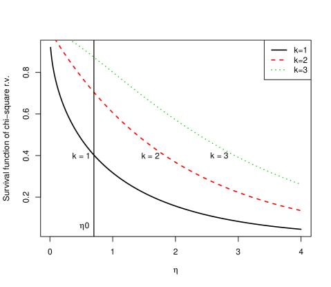
One limitation of statistic is that, if degree of freedom are too small, the approximation to the distribution would fail. For example, . Since test of small degree of freedom (denotes it by ) did not have enough power (namely is not large enough). That is to say, for a r.v. , the p-value is defined by
which tends to be small when varies from 3 to 1. An attempt at this has been made in the figure below.
Another drawback is that, with small number of class , Haberman (1988) discussed that: “chi-squared test statistics may be asymptotically inconsistent even in cases in which a satisfactory chi-squared approximation exists for the distribution under the null hypothesis.”
Consequently, a better way of comparing distributions is to use a non-parametric test not depending on the parametric assumption of the models. One of notable non-parametric test is Kolmogorov-Smirnov test by using following statistic:
which is a nonparametric test of continuous distributions. And it could be modified for discrete distribution:
where ’s are the discontinuity points ( is the countable index set).
Fortunately, Arnold and Emerson (2011) developed the R package “dgof”, which can calculate Kolmogorov-Smirnov test of the discrete distribution. The non-parametric test avoids the assumption of parametric model, hence it is an effective way to evaluate different distributions’ performance.
6 Applications with simulated and real data
In this section, we will describe four examples of fitting data by CMNB distribution, and we will compare them with those by the negative binomial and COM-Poisson distribution. The notations, CMNB, NB and CMP distribution, in the following tables, are representing the CMNB, negative binomial and COM-Poisson, respectively. By using scoring method in section 5.2, we could estimated the CMNB distribution with three parameters. The original and expected frequencies, parameter estimators (obtained by maximum likelihood method), the and K-S statistics, and corresponding -values. are all being considered in the tables below.
6.1 Simulated Data
In this subsection, the inverse method mentioned in section 4 were used to generate random variables from CMNB, NB and COM-Poisson distribution with certain parameters. And we compare the performance of the fit by CMNB, NB and COM-Poisson distribution.
Example 1. As our first simulation example, we consider the original data that are following the NB distribution. We use inverse method to draw 10000 random samples from NB distribution with parameter , and fit the data with above-mentioned distributions, the results are shown in the following table 1.
| Sample values | Frequency | Fitted Values | ||
| CMNB | NB | CMP | ||
| 0 | 5060 | 5054 | 5049 | 5019 |
| 1 | 2480 | 2494 | 2492 | 2502 |
| 2 | 1199 | 1237 | 1236 | 1248 |
| 3 | 638 | 615 | 614 | 622 |
| 4 | 318 | 306 | 306 | 310 |
| 5 | 165 | 152 | 152 | 155 |
| 6 | 74 | 76 | 76 | 77 |
| 7 | 33 | 38 | 38 | 38 |
| 8 | 20 | 19 | 19 | 19 |
| 9 | 8 | 9 | 9 | 10 |
| 10 | 4 | 5 | 5 | 5 |
| 11 | 1 | 2 | 2 | 2 |
| Total | 10000 | 10007 | 9998 | 10007 |
| par1 | 0.97 | 0.99 | 0.50 | |
| par2 | 1.00 | 0.50 | 0.00 | |
| par3 | 0.51 | |||
| 5.29 | 5.44 | 5.83 | ||
| d.f. of | 8.00 | 9.00 | 9.00 | |
| p value of | 0.73 | 0.79 | 0.76 | |
| K-S | 0.002199 | 0.003976 | 0.004451 | |
| p value of K-S | 1.000000 | 0.997435 | 0.988831 | |
In this case, although the data are generated from NB distribution, the CMNB distribution can also be recognized as the true distribution, as the estimator of is 1. That is to say, the data can be seen negative binomial distributed, and note that he result of test and K-S test is nearly the same, all of these indicate that the CMNB distribution is an extension of NB distribution.
Example 2. In this example, we will evaluate the performance of NB distribution, when the original data are generated from CMNB distribution. Assume are independent and identically CMNB distributed random variables with parameters . Let and , we can generate sample points through inverse method introduced in section 4. The fitting results are summarized below:
| Sample values | Frequency | Fitted Values | ||
| CMNB | NB | CMP | ||
| 0 | 6442 | 6449 | 6421 | 5937 |
| 1 | 1866 | 1878 | 1951 | 2413 |
| 2 | 874 | 869 | 837 | 981 |
| 3 | 435 | 415 | 394 | 399 |
| 4 | 188 | 201 | 194 | 162 |
| 5 | 101 | 98 | 98 | 66 |
| 6 | 55 | 48 | 50 | 27 |
| 7 | 19 | 24 | 26 | 11 |
| 8 | 7 | 12 | 14 | 4 |
| 9 | 8 | 6 | 7 | 2 |
| 10 | 2 | 3 | 4 | 1 |
| 11 | 2 | 1 | 2 | 0 |
| 12 | 1 | 1 | 1 | 0 |
| Total | 10000 | 10005 | 9999 | 10003 |
| par1 | 0.01 | 0.55 | 0.41 | |
| par2 | 0.12 | 0.45 | 0.00 | |
| par3 | 0.50 | 0.44 | ||
| 7.26 | 16.38 | 281.94 | ||
| d.f. of | 9.00 | 10.00 | 10.00 | |
| p value of | 0.61 | 0.09 | 0.00 | |
| K-S | 0.001484 | 0.006484 | 0.050678 | |
| p value of K-S | 1.000000 | 0.794579 | 0.000000 | |
From table 2, we note first that in test, the CMNB distribution’s statistic 7.26 is dramatically smaller than NB distribution’s 16.38, while the corresponding p-values are 0.61 and 0.09 respectively, which implies that NB distribution may not be a reasonable fit. As for the result of the K-S test, it suggests that CMNB distribution performs best, because the p-value of CMNB distribution is approximately 1, while NB’s and COM-Poisson’s are 0.79 and 0.
6.2 Real data analysis
In this subsection, the distributions mentioned above are considered here to analyze real actuarial claim data that have ultrahigh zero-inflated and overdispersion properties, then compare its Kolmogorov-Smirnov test and Chi-squared test.
Example 3. Let us consider the claim counts of the third party liability vehicle insurance (see Willmot (1987) for data set in an Zaire insurance company) which correspond to claims from 4000 vehicle policies. Gómez-Déniz (2014) analyzed the data using negative binomial distribution and found that it is a reasonable fit. We analyze the data by CMNB, NB and CMP distribution, and the results are summarized below:
| No. of claims | Frequency | Fitted Values | ||
| CMNB | NB | CMP | ||
| 0 | 3719 | 3720 | 3719 | 3681 |
| 1 | 232 | 231 | 230 | 294 |
| 2 | 38 | 39 | 40 | 23 |
| 3 | 7 | 8 | 8 | 2 |
| 4 | 3 | 2 | 2 | 0 |
| 5 | 1 | 1 | 0 | 0 |
| Total | 4000 | 4001 | 3999 | 3991 |
| par1 | 0.57 | 0.22 | 0.08 | |
| par2 | 3.06 | 0.71 | 0.00 | |
| par3 | 0.35 | |||
| 1.01 | 1.56 | 173.28 | ||
| d.f. of | 2.00 | 3.00 | 3.00 | |
| p value of | 0.60 | 0.67 | 0.00 | |
| K-S | 0.000250 | 0.000500 | 0.009500 | |
| p value of K-S | 1.000000 | 1.000000 | 0.863178 | |
It’s a well known fact that NB distribution is a popular choice to fit the claim data in actuarial science. However findings in Table 3 suggest that, CMNB might be a better choice for fitting this data. It appears that, for chi-square statistic, fitting the chi-square statistic with the NB distribution, it turns out to be , which is dramatically larger than CMNB’s , and the p-values correspond to the statistics is nearly the same. As for Kolmogorov-Smirnov test, although the p-value is both 1, it still can be seen that the K-S statistic of CMNB is slightly smaller than NB’s. All of these show that the CMNB is superior to the fit the data.
Example 4. For this example, we use the car insurance claim data of a Chinese insurance company (see Wang and Lei, (2000)), which were modeled with negative binomial distribution. Total insurance policies are . We analyze the data with the above-mentioned distributions, and the results are shown in table 4.
| No. of Claims | Frequency | Fitted Values | ||
| CMNB | NB | CMP | ||
| 0 | 27141 | 27177 | 27166 | 26599 |
| 1 | 5789 | 5666 | 5664 | 6430 |
| 2 | 1443 | 1554 | 1563 | 1554 |
| 3 | 457 | 466 | 467 | 376 |
| 4 | 155 | 146 | 145 | 91 |
| 5 | 56 | 47 | 46 | 22 |
| 6 | 27 | 15 | 15 | 5 |
| 7 | 2 | 5 | 5 | 1 |
| 8 | 1 | 2 | 2 | 0 |
| 9 | 1 | 1 | 1 | 0 |
| Total | 35072 | 35079 | 35074 | 35078 |
| par1 | 0.95 | 0.61 | 0.24 | |
| par2 | 10.40 | 0.66 | 0.00 | |
| par3 | 0.36 | |||
| 24.16 | 27.88 | 300.60 | ||
| d.f. of | 6.00 | 7.00 | 7.00 | |
| p value of | 0.00 | 0.00 | 0.00 | |
| K-S | 0.002667 | 0.002905 | 0.015584 | |
| p value of K-S | 0.964199 | 0.928729 | 0.000000 | |
As can be observed from table 4, CMNB is the clear winner. CMNB distribution outperforms other distributions by either test or K-S test, as statistic and K-S statistic of CMNB is slightly smaller than that of NB’s, and dramatically smaller than CMP’s. It shows that their performance is on the whole dominated by CMNB distribution.
7 Further researches
Many discrete distributions in aspects of related statistical models are widely proposed in plenty of research articles. The CMNB distribution can be used in driving count data in some generalized linear models (GLMs). For example, Poisson regression, COM-Poisson regression and negative binomial regression (NBR), whose driving distribution of count data are actually the special case or limiting case of CMNB distribution, see Figure 2 for a visual relations. Even in the popular logistic regression, the assuming distribution lying in this model is Bernoulli distribution which is a limiting case of COM-Poisson distribution. Besides GLMs, high-dimensional GLMs (i.e., the sample size may be greater than the number of covariates ) should also be considered for CMNB, see Zhang and Jia (2017) and references therein for high-dimensional NBR. The discrete frailty item as a random effect in survival analysis model (or Long-term survival models, see Rodrigues et al. (2012)), which could be considered to set some flexible distributions. Besides the researches of regression model, in our paper, both conditional distribution and Stein identity characterizations are obtained. Test of statistic based on the novel characterization is more reasonable, since that the distribution-free and omnibus goodness-of-fit test like Kolmogorov-Smirnov and Chi-squared does not depend on certain types(or families) of distributions, may have their own drawbacks. For example, some new tests of a class of count distributions which includes the Poisson is constructed from Stein identity characterization (see Meintanis and Nikitin (2008)), and some tests of logarithmic series distribution comes from conditional distribution characterization (see Ramalingam and Jagbir (1984)). The goodness-of-fit tests between two continuous probability distributions based on combining Stein s identity is studied by Liu, Lee and Jordan (2016), and we consider study Stein discrepancy goodness-of-fit tests for discrete distribution in the future.
8 Acknowledgments
The proposed COM-negative binomial distribution of this work was as early as conceptualized in Dec. 2014 when the authors saw the online version of Imoto (2014). The authors want to thank Prof. Köhler R. for mailing the valuable encyclopedia of discrete univariate distributions (Wimmer and Altmann (1999)) to us. This work was partly supported by the National Natural Science Foundation of China (No.11201165).
9 References
References
- Arnold and Emerson (2011) Arnold, T. B., Emerson, J. W. (2011). Nonparametric goodness-of-fit tests for discrete null distributions. The R Journal, 3(2), 34-39.
- Bohning (2016) Bohning, D. (2016). Ratio plot and ratio regression with applications to social and medical sciences. Statistical Science, 31(2), 205-218.
- Borges et al. (2014) Borges, P., Rodrigues, J., Balakrishnan, N., Baz n, J. (2014). A COM-Poisson type generalization of the binomial distribution and its properties and applications. Statistics & Probability Letters, 87, 158-166.
- Brown and Phillips (1999) Brown, T. C., Phillips, M. J. (1999). Negative binomial approximation with Stein’s method. Methodology and Computing in Applied Probability, 1(4), 407-421.
- Brown and Xia (2001) Brown, T. C., Xia, A. (2001). Stein’s method and birth-death processes. Annals of probability, 29(3), 1373-1403.
- Chakraborty and Ong (2016) Chakraborty, S., Ong, S. H. (2016). A COM-Poisson-type generalization of the negative binomial distribution. Communications in Statistics-Theory and Methods, 45(14), 4117-4135.
- Chakraborty and Imoto (2016) Chakraborty, S., Imoto, T. (2016). Extended Conway-Maxwell-Poisson distribution and its properties and applications. Journal of Statistical Distributions and Applications, 3(1), 5.
- Conway and Maxwell (1962) Conway, R. W., Maxwell, W. L. (1962). A queuing model with state dependent service rates. Journal of Industrial Engineering, 12(2), 132-136.
- Deng and Tan (2009) Deng, Z., Tan, Z. (2009). Fitting three-parameter Poisson-Tweedie model to claim frequency and test the location parameter. Mathematical Theory and Applications, 29(1), 51-55. (in Chinese) http://en.cnki.com.cn/Article_en/CJFDTotal-LLYY200901014.htm
- Denuit (1997) Denuit, M. (1997). A new distribution of Poisson-type for the number of claims. Astin Bulletin, 27(02), 229-242.
- Denuit et al. (2007) Denuit, M., Maréchal, X., Pitrebois, S., Walhin, J. F. (2007). Actuarial modelling of claim counts: Risk classification, credibility and bonus-malus systems. Wiley.
- Gómez-Déniz (2011) Gómez-Déniz, E., Sarabia, José María, Calderín-Ojeda, E. (2011). A new discrete distribution with actuarial applications. Insurance: Mathematics and Economics, 48(3), 406-412
- Gómez-Déniz (2014) Gómez-Déniz, E., Calderín-Ojeda, E. (2014). Unconditional distributions obtained from conditional specification models with applications in risk theory. Scandinavian Actuarial Journal, 2014(7), 602-619.
- Gupta et al. (2014) Gupta, R. C., Sim, S. Z., Ong, S. H. (2014). Analysis of discrete data by Conway-Maxwell Poisson distribution. AStA Advances in Statistical Analysis, 1-17.
- Haberman (1988) Haberman, S. J. (1988). A warning on the use of chi-squared statistics with frequency tables with small expected cell counts. Journal of the American Statistical Association, 83(402), 555-560.
- Ibragimov (1956) Ibragimov, I. D. A. (1956). On the composition of unimodal distributions. Theory of Probability & Its Applications, 1(2), 255-260.
- Imoto (2014) Imoto, T. (2014). A generalized Conway-Maxwell-Poisson distribution which includes the negative binomial distribution. Applied Mathematics and Computation, 247, 824-834.
- Johnson et al. (2005) Johnson, N. L., Kemp, A. W., Kotz S. (2005). Univariate discrete distributions, 3rd. Wiley.
- Kadane (2016) Kadane, J. B. (2016). Sums of possibly associated Bernoulli variables: The Conway-Maxwell-Binomial distribution. Bayesian Analysis, 11(2), 403-420.
- Kagan et al. (1973) Kagan, A. M., Linnik, Y. V., Rao, C. R. (1973). Characterization problems in mathematical statistics, Wiley.
- Kaas (2008) Kaas, R., Denuit, M., Dhaene, J., Goovaerts, M. (2008). Modern Actuarial Risk Theory Using R, Second Edition. Springer, Berlin.
- Kokonendji et al. (2008) Kokonendji, C. C., Mizere, D., Balakrishnan, N. (2008). Connections of the Poisson weight function to overdispersion and underdispersion. Journal of Statistical Planning and Inference, 138(5), 1287-1296.
- Liu, Lee and Jordan (2016) Liu, Q., Lee, J., Jordan, M. (2016). A kernelized Stein discrepancy for goodness-of-fit tests. In International Conference on Machine Learning (pp. 276-284).
- Meintanis and Nikitin (2008) Meintanis, S. G., Nikitin, Y. Y. (2008). A class of count models and a new consistent test for the Poisson distribution. Journal of Statistical Planning and Inference, 138(12), 3722-3732.
- Patil and Seshadri (1964) Patil, G. P., Seshadri, V. (1964). Characterization theorems for some univariate probability distributions. Journal of the Royal Statistical Society. Series B (Methodological), 286-292.
- Rao and Rubin (1964) Rao, C. R., Rubin, H. (1964). On a characterization of the Poisson distribution. Sankhyā: The Indian Journal of Statistics, Series A, 295-298.
- Rényi (1961) Rényi, A. (1961). On measures of entropy and information. In Fourth Berkeley symposium on mathematical statistics and probability (Vol. 1, pp. 547-561).
- Ramalingam and Jagbir (1984) Ramalingam, S., Jagbir, S. (1984). A characterization of the logarithmic series distribution and its application. Communications in Statistics-Theory and Methods, 13(7), 865-875.
- Rodrigues et al. (2012) Rodrigues, J., de Castro, M., Cancho, V. G., Balakrishnan, N. (2009). COM-Poisson cure rate survival models and an application to a cutaneous melanoma data. Journal of Statistical Planning and Inference, 139(10), 3605-3611.
- Sellers et al. (2012) Sellers, K. F., Borle, S., Shmueli, G. (2012). The COM-Poisson model for count data: a survey of methods and applications. Applied Stochastic Models in Business and Industry, 28(2), 104-116.
- Shaked and Shanthikumar (2007) Shaked, M., Shanthikumar, J. G. (2007). Stochastic orders. Springer.
- Shanbhag (1977) Shanbhag, D. N. (1977). An extension of the Rao-Rubin characterization of the Poisson distribution. Journal of Applied Probability, 640-646.
- Shmueli et al. (2005) Shmueli, G., Minka, T. P., Kadane, J. B., Borle, S., Boatwright, P. (2005). A useful distribution for fitting discrete data: revival of the Conway-Maxwell-Poisson distribution. Journal of the Royal Statistical Society: Series C (Applied Statistics), 54(1), 127-142.
- Steutel (1970) Steutel, F. W. (1970). Preservation of infinite divisibility under mixing and related topics. MC Tracts, 33, 1-99.
- Steutel and van Harn (2003) Steutel, F. W., Van Harn, K. (2003). Infinite divisibility of probability distributions on the real line. CRC Press, New York.
- Tsallis (1988) Tsallis, C. (1988). Possible generalization of Boltzmann-Gibbs statistics. Journal of statistical physics, 52(1-2), 479-487.
- Temme (2011) Temme, N. M. (2011). Special functions: An introduction to the classical functions of mathematical physics. Wiley.
- Wang and Lei, (2000) Wang, L.M., Lei, Y.L., (2000). Simulation and EM algorithm for the distribution of number of claim in the heterogeneous portfolio. Communications on Applied Mathematics and Computational Science. 14(2) pp. 71-78.
- Willmot (1987) Willmot, G. E. (1987). The Poisson-inverse Gaussian distribution as an alternative to the negative binomial. Scandinavian Actuarial Journal, 1987(3-4), 113-127.
- Wimmer et al. (1995) Wimmer, G., Köhler, R., Grotjahn, R., Altmann, G. (1994). Towards a theory of word length distribution. Journal of Quantitative Linguistics, 1(1), 98-106.
- Wimmer and Altmann (1999) Wimmer, G., Altmann, G. (1999). Thesaurus of univariate discrete probability distributions. Stamm.
- Zhang et al. (2014) Zhang, H., Liu, Y., Li, B. (2014). Notes on discrete compound Poisson model with applications to risk theory. Insurance: Mathematics and Economics, 59, 325-336.
- Zhang and Li (2016) Zhang, H., Li, B. (2016). Characterizations of discrete compound Poisson distributions. Communications in Statistics-Theory and Methods, 45(22), 6789-6802.
- Zhang et al. (2017) Zhang, H., Li, B., Kerns, G. J. (2017). A characterization of signed discrete infinitely divisible distributions. Studia Scientiarum Mathematicarum Hungarica, 54(4), 446-470.
- Zhang and Jia (2017) Zhang, H., & Jia, J. (2017). Elastic-net regularized High-dimensional Negative Binomial Regression: Consistency and Weak Signals Detection. arXiv preprint arXiv:1712.03412.
- Zygmund (2002) Zygmund, A. (2002). Trigonometric series. Cambridge University Press, Cambridge.