The wrapped skew Gaussian process for analyzing spatio-temporal data

Abstract

We consider modeling of angular or directional data viewed as a linear variable wrapped onto a unit circle. In particular, we focus on the spatio-temporal context, motivated by a collection of wave directions obtained as computer model output developed dynamically over a collection of spatial locations. We propose a novel wrapped skew Gaussian process which enriches the class of wrapped Gaussian process. The wrapped skew Gaussian process enables more flexible marginal distributions than the symmetric ones arising under the wrapped Gaussian process and it allows straightforward interpretation of parameters. We clarify that replication through time enables criticism of the wrapped process in favor of the wrapped skew process.
We formulate a hierarchical model incorporating this process and show how to introduce appropriate latent variables in order to enable efficient fitting to dynamic spatial directional data. We also show how to implement kriging and forecasting under this model. We provide a simulation example as a proof of concept as well as a real data example. Both examples reveal consequential improvement in predictive performance for the wrapped skew Gaussian specification compared with the earlier wrapped Gaussian version.

Keywords: Directional data Hierarchical model Kriging Markov chain Monte Carlo Space-time data Wave directions

1 Introduction

There is increasing interest in analyzing directional data which are collected over space and time. Examples arise, for instance, in oceanography (wave directions), meteorology (wind directions), biology (study of animal movement). They also arise from periodic data, e.g., event times might be wrapped according to a daily period to give a circular view (eliminating end effects). We wrap time around a circle by a modulus transformation and, without loss of generality, can rescale to degrees or angles on a unit circle. Time wrapping with spatial data occurs naturally in applications such as locations and times of crime events, locations and times of automobile accidents, and residence address with time of admission for hospitalizations.

Jona Lasinio et al (2012) introduced a Bayesian hierarchical model to handle angular data, enabling full inference regarding all model parameters and prediction under the model. Their context was multivariate directional observations arising as angular data measurements taken at spatial locations, anticipating structured dependence between these measurements. They proposed the wrapped spatial Gaussian process, induced from a linear spatial Gaussian process. They explored dependence structure and showed how to implement kriging of mean directions and concentrations in this setting.

The current state of the art for modeling circular space-time data includes the wrapped Gaussian process and the projected Gaussian process. The second, although more flexible, is based upon a four parameter model such that complex interactions among the parameters make interpretation difficult. In this paper our contribution is to overcome a key limitation of the wrapped Gaussian process, that the marginal distributions at all locations are symmetric. Here we introduce the wrapped skew Gaussian process. This new circular process allows for asymmetric marginal distributions while retaining straightforward parametric interpretation. Our wrapping approach is developed from the skew normal distribution proposed by Azzalini (1985) and the process extension constructed by Zhang et al (2010)

By now, there is a fairly rich literature on skew multivariate normal models (Azzalini, 2005; Sahu et al, 2003; Ma and Genton, 2004; Wang et al, 2004) but all are inline, i.e., on a linear scale. The first attempt to wrap the skew normal distribution for circular data can be found in Pewsey (2000) where its basic properties are derived. Follow-on work appears in Pewsey (2006); Hernández-Sánchez and Scarpa (2012).

To our knowledge, we propose the first extension to multivariate wrapped skew distributions, in particular, to a spatial and spatio-temporal setting. In what follows we review the univariate wrapped skew normal distribution, showing the flexibility of shapes and do the same for bivariate wrapped skew normal distributions. Then, we turn to a hierarchical model for dynamic spatial data and show how, using suitable latent variables, to fit it efficiently. We also show how to implement kriging under this model.

A critical point emerges: though we can fit both models with a single sample of spatially referenced directions, in terms of kriging performance, we can not criticize the wrapped spatial Gaussian process in favor of the wrapped skew spatial Gaussian process. This is not surprising. Consider the linear situation. With a single sample of data from a set of locations, it is difficult to criticize the Gaussian process in favor of a more complex stochastic process specification, i.e., it is difficult to criticize a multivariate normal model with a single sample of multivariate data. However, with replicates, we are able to demonstrate substantially improved predictive performance for the wrapped skew Gaussian process. We do this both with simulated data, as a proof of concept, and with real data, making direct comparison. In our setting replicates arise through a dynamic spatial data where we envision i.i.d. spatial increment processes.

Inference for spatial data is challenging due to the restriction of support to the unit circle, $[0,2\pi)$, and to the sensitivity of descriptive and inferential results to the starting point on the circle. There exists a substantial early literature on circular data (see e.g. Mardia (1972) and Mardia and Jupp (1999), Jammalamadaka and SenGupta (2001) or Fisher (1996)) primarily confined to descriptive statistics and limited inference for simple univariate models.

Computational procedures such as MCMC methods and the EM algorithm, have substantially advanced inference opportunities for directional data. Some examples include linear models (Harrison and Kanji, 1988; Fisher, 1996; Kato and Shimizu, 2008), linear models in a Bayesian context (Guttorp and Lockhart, 1988; Damien and Walker, 1999), models for circular time series (Breckling, 1989; Coles, 1998; Mardia and Jupp, 1999; Ravindran and Ghosh, 2011; Hughes, 2007; Fisher and Lee, 1992; Holzmann et al, 2006) or model for space-time circular-linear data (Lagona et al, 2015). Recently, Kato (2010), building upon earlier work (Kato et al, 2008), proposed a discrete time Markov process for circular data. He uses the Möbius circle transformation, connecting it with an early Markov process model of Fisher and Lee (1994).

With regard to multivariate theory for circular data, particularly in the fully Bayesian setting, the work of Coles (1998) is foundational for ours. He also employs wrapped distributions, noting that, in the Gaussian case, they can be readily given a multivariate extension. Coles mostly works with independent replicates of multivariate circular data in low dimension with an unknown covariance matrix and develops some theory and examples for the time series setting. He mentions possible extensions to the spatial setting but offers no development, in particular, no thoughts on regression or kriging (Sections 3.5 and 3.6 below). Coles and Casson (1998) include spatial dependence in looking at the direction of maximum wind speed. With little detail, they propose conditionally independent directions modeled with a von Mises distribution, introducing spatial structure in the modal direction and concentration parameters, a second stage specification. Our view, again following Jona Lasinio et al (2012), is to introduce spatial structure at the first stage of the modeling, directly on the angular variables, resulting in a spatial process model with smooth process realizations.

Following a different strand, the projected normal and the associated projected Gaussian process (Wang and Gelfand, 2013, 2014) have generated recent interest. In particular, a general bivariate normal distribution is projected to an angle, extending work of Presnell et al (1998) and Nuñez-Antonio and Gutiérrez-Peña (2005). The extension to a stochastic process for variables on the circle over a continuous spatial domain, the projected Gaussian process, is induced from a linear bivariate spatial Gaussian process. The projected Gaussian process has marginal distributions that can be asymmetric, possibly bimodal, an advantage over the wrapped Gaussian process. Wang and Gelfand (2014) also investigate properties of this process, including the nature of joint distributions for pairs of directions at different locations. Working within a hierarchical Bayesian framework, they show that model fitting is straightforward using suitable latent variable augmentation in the context of Markov chain Monte Carlo (MCMC). In very recent work, Mastrantonio et al (2015) offer comparison between the wrapping and the projection modeling approaches.

We remark that we have explored the possibility of introducing skewness into the projected Gaussian process. The overall process model is induced by a bivariate skewed Gaussian process. This is a more challenging process to work with; the resulting directional process model is extremely messy and has proved very difficult to fit. It likely exceeds what the data is capable of supporting. We do not discuss it further.

Our motivating example is drawn from marine data. Wave heights and outgoing wave directions, the latter being measured in degrees relative to a fixed orientation, are the main outputs of marine forecasts. Numerical models for weather and marine forecasts need statistical post-processing. Wave directions, being angular variables, cannot be treated through standard post-processing techniques (see Engel and Ebert, 2007; Bao et al, 2009, and references therein). In Bao et al (2009) bias correction and ensemble calibration forecasts of surface wind direction are proposed. The authors use circular-circular regression as in Kato et al (2008) for bias correction and Bayesian model averaging with the von Mises distribution for ensemble calibration. However, their approach does not explicitly account for spatial structure.

Lastly, it is worth commenting that, in our setting, wave direction data is viewed differently from wind direction data. The former is only available as an angle while the latter is customarily associated with wind speed, emerging as the resultant of North-South and East-West wind speed components.

The format of the paper is as follows. In Section 2 we review, develop and illustrate the univariate wrapped skew normal distribution. Section 3 extends to the wrapped skew Gaussian process, including distribution theory, model fitting, and kriging. Section 4 provides the dynamic version which we then pursue through simulation in Section 5 and a wave direction data analysis in Section 6. Section 7 offers a brief summary and some future research possibilities.

2 The wrapped skew normal

2.1 The univariate case

We begin with the univariate wrapped skew normal distribution. Let $X$ and $W$ be two independent standard normal variables, let $\sigma^{2}\in\mathbb{R}^{+}$ and $\lambda\in\mathbb{R}$. Then, the random variable

$$Z=\mu+\frac{\sigma\lambda}{\sqrt{1+\lambda^{2}}}|X|+\frac{\sigma}{\sqrt{1+\lambda^{2}}}W-\frac{\sigma\lambda\sqrt{2}}{\sqrt{\pi(1+\lambda^{2})}}$$ (1)

is said to be distributed as a skew normal variable (Azzalini, 1985) with parameters $\mu$, $\sigma^{2}$ and $\lambda$; i.e., $Z|\boldsymbol{\Psi}\sim SN(\mu,\sigma^{2},\lambda)$, where $\boldsymbol{\Psi}$ denotes the vector of parameters. Let $\phi(\cdot)$ and $\Phi(\cdot)$ be the probability density function (pdf) and the cumulative density function (cdf), respectively, of a standard normal. Then, the pdf of $Z|\boldsymbol{\Psi}$ is

$$\frac{2}{\sigma}\phi\left(\frac{z-\mu+\frac{\sigma\lambda\sqrt{2}}{\sqrt{\pi(1+\lambda^{2})}}}{\sigma}\right)\Phi\left(\lambda\left(\frac{z-\mu+\frac{\sigma\lambda\sqrt{2}}{\sqrt{\pi(1+\lambda^{2})}}}{\sigma}\right)\right)$$ (2)

and from (1) we can easily derive the mean and the variance of $Z$, respectively. They are $\mu$ (the definition in (1) was made in order to center $Z$ at $\mu$) and

$${\sigma^{2}\lambda^{2}}/{({1+\lambda^{2}})}\left(1-{2}/{\pi}\right)+{\sigma^{2}}/{({1+\lambda^{2}})}.$$

With the transformation

$$\Theta=Z\mbox{ mod }2\pi,\hskip 5.69046pt\mbox{implying }\Theta\in[0,2\pi),$$ (3)

we obtain a random variable with support on the unit circle. We can express the inline variable as $Z=\Theta+2\pi K$, where $K$, the winding number, assumes values in $\mathbb{Z}=\{0,\pm 1,\pm 2,...\}$. The transformation (3) defines what is called a wrapped skew normal (WSN) distribution, as introduced in Pewsey (2000). It wraps the skew normal distribution, defined on the real line, onto the unit circle. Details on the wrapping approach can be found in Jammalamadaka and SenGupta (2001) or Mardia and Jupp (1999).

The pdf of $\Theta|\boldsymbol{\Psi}$ is

$$\sum_{k\in\mathbb{Z}}\frac{2}{\sigma} \phi\left(\frac{\theta+2\pi k-\mu+\frac{\sigma\lambda\sqrt{2}}{\sqrt{\pi(1+\lambda^{2})}}}{\sigma}\right)$$ (4)

$$\times\Phi\left(\lambda\left(\frac{\theta+2\pi k-\mu+\frac{\sigma\lambda\sqrt{2}}{\sqrt{\pi(1+\lambda^{2})}}}{\sigma}\right)\right).$$ (5)

The infinite sum in (5) is impossible to evaluate but, to display the density, as with the wrapped normal case, we can obtain an accurate approximation by appropriately truncating the sum. Figure 1 illustrates the effect of introduction of skewness into the wrapped normal density. To obtain a sample from a wrapped skew normal we first obtain a sample from the skew normal and then transform it to a circular variable via (3). Also, note that, if we let $K$ be a random variable, the density inside the sum in (5) is the joint density of $(\Theta,K|\boldsymbol{\Psi})$ whence, we marginalize over $K$ to obtain the density of the circular variable.

Figure 1: Densities of the wrapped skew normal (solid line) with $\mu=\pi$, $\sigma^{2}=1$ and different values of $\lambda$ along with the associated densities of the wrapped normal (dashed line) having the same circular mean and variance

(a) $\lambda=3$

(b) $\lambda=10$

(c) $\lambda=-10$

Pewsey (2000) gives the fundamental properties of the WSN along with closed forms for the cosine and sine moments. Let $\mu^{*}=\mu-\frac{\sigma\lambda\sqrt{2}}{\sqrt{\pi(1+\lambda^{2})}}$ and $\mathcal{J}(a)=\int_{0}^{a}\sqrt{\frac{2}{\pi}}\exp\left(\frac{u^{2}}{2}\right)du$ the cosine and sine moments become

$$\alpha_{p} =E(\cos p\Theta|\boldsymbol{\Psi})=\exp\left(-\frac{{p^{2}}\sigma^{2}}{2}\right)$$ (6)

$$\times\left(\cos(p\mu^{*})-\mathcal{J}\left(\frac{\lambda\sigma p}{\sqrt{1+\lambda^{2}}}\right)\sin(p\mu^{*})\right)$$ (7)

and

$$\beta_{p} =E(\sin p\Theta|\boldsymbol{\Psi})=\exp\left(-\frac{{p^{2}}\sigma^{2}}{2}\right)$$ (8)

$$\times\left(\sin(p\mu^{*})+\mathcal{J}\left(\frac{\lambda\sigma p}{\sqrt{1+\lambda^{2}}}\right)\cos(p\mu^{*})\right).$$ (9)

The trigonometric moments (7) and (9) are useful to compute the circular mean of $\Theta$, $\tilde{\mu}=\mbox{atan}^{*}\frac{\alpha_{1}}{\beta_{1}}$, and the circular concentration, $\tilde{c}=\sqrt{\alpha_{1}^{2}+\beta_{1}^{2}}$. However, unfortunately we need to compute $\mathcal{J}(\cdot)$, which is not available in closed form. Pewsey (2000) suggests to use deterministic numerical integration methods but we note that $\alpha_{p}$ and $\beta_{p}$ can be computed using Monte Carlo approximation.

Indeed, from (1) we can see that

$$Z|X,\boldsymbol{\Psi}\sim N\left(\mu+\frac{\sigma\lambda}{\sqrt{1+\lambda^{2}}}|X|-\frac{\sigma\lambda\sqrt{2}}{\sqrt{\pi(1+\lambda^{2})}},\frac{\sigma^{2}}{1+\lambda^{2}}\right)$$ (10)

and as a consequence

$$\Theta|X,\boldsymbol{\Psi}\sim WN\left(\mu+\frac{\sigma\lambda}{\sqrt{1+\lambda^{2}}}|X|-\frac{\sigma\lambda\sqrt{2}}{\sqrt{\pi(1+\lambda^{2})}},\frac{\sigma^{2}}{1+\lambda^{2}}\right),$$ (11)

where $WN(\cdot)$ indicates the wrapped normal distribution. Let $\{X^{b}\}_{b=1}^{B}$ be a set of $B$ samples from the distribution of $X$. Then, we can write the cosine moments as $\alpha_{p}=E(\cos p\Theta|\boldsymbol{\Psi})=E_{X|\boldsymbol{\Psi}}E_{\Theta|X,\boldsymbol{\Psi}}(\cos p\Theta|X,\boldsymbol{\Psi})$, since $E_{\Theta|X,\boldsymbol{\Psi}}(\cos p\Theta|X,\boldsymbol{\Psi})$ is the cosine moment of $\Theta|X,\boldsymbol{\Psi}$. Following Jona Lasinio et al (2012), a Monte Carlo approximation of $\alpha_{p}$ is

$$\hat{\alpha}_{p} \approx\frac{\exp\left(-p^{2}\frac{\sigma^{2}}{2(1+\lambda^{2})}\right)}{B}$$ (12)

$$\times\sum_{b=1}^{B}\cos\left(p\left(\mu+\frac{\sigma\lambda}{\sqrt{1+\lambda^{2}}}|X|-\frac{\sigma\lambda\sqrt{2}}{\sqrt{\pi(1+\lambda^{2})}}\right)\right).$$ (13)

Similarly, we find

$$\hat{\beta}_{p} \approx\frac{\exp\left(-p^{2}\frac{\sigma^{2}}{2(1+\lambda^{2})}\right)}{B}$$ (14)

$$\times\sum_{b=1}^{B}\sin\left(p\left(\mu+\frac{\sigma\lambda}{\sqrt{1+\lambda^{2}}}|X|-\frac{\sigma\lambda\sqrt{2}}{\sqrt{\pi(1+\lambda^{2})}}\right)\right)$$ (15)

and then $\hat{\tilde{\mu}}=\mbox{atan}^{*}\frac{\hat{\alpha}_{1}}{\hat{\beta}_{1}}$ and $\hat{\tilde{c}}=\sqrt{\hat{\alpha}_{1}^{2}+\hat{\beta}_{1}^{2}}$.

2.2 The bivariate case

Let $Z_{1}$ and $Z_{2}$ be two random variables skew normal distributed with, respectively, parameters $(\mu_{1},\sigma_{1}^{2},\lambda_{1})$ and $(\mu_{2},\sigma_{2}^{2},\lambda_{2})$:

$$Z_{1} =\mu_{1}+\frac{\sigma_{1}\lambda_{1}}{\sqrt{1+\lambda_{1}^{2}}}|X_{1}|+\frac{\sigma_{1}}{\sqrt{1+\lambda_{1}^{2}}}W_{1}-\frac{\sigma_{1}\lambda_{1}\sqrt{2}}{\sqrt{\pi(1+\lambda_{1}^{2})}},$$ (16)

$$Z_{2} =\mu_{2}+\frac{\sigma_{2}\lambda_{2}}{\sqrt{1+\lambda_{2}^{2}}}|X_{2}|+\frac{\sigma_{2}}{\sqrt{1+\lambda_{2}^{2}}}W_{2}-\frac{\sigma_{2}\lambda_{2}\sqrt{2}}{\sqrt{\pi(1+\lambda_{2}^{2})}}.$$ (17)

We introduce dependence between $Z_{1}$ and $Z_{2}$ by letting $\mbox{Cor}(X_{1},X_{2}|\boldsymbol{\Psi})=\rho_{x}$ and $\mbox{Cor}(W_{1},W_{2}|\boldsymbol{\Psi})=\rho_{w}$. Then, we say that $(Z_{1},Z_{2}|\boldsymbol{\Psi})$ is distributed as a bivariate skew normal with the additional parameters, $\rho_{x}$ and $\rho_{w}$. This specification of the bivariate skew normal, due to Zhang and El-Shaarawi (2010), differs from the one that can be derived using the multivariate normal of Azzalini and Valle (1996) and it is more suitable to built a stationary process, see Section 3.

Using the transformation (3) we can obtain the circular variables $\Theta_{1}=Z_{1}\mbox{ mod }2\pi$ and $\Theta_{2}=Z_{2}\mbox{ mod }2\pi$ associated with $(Z_{1},Z_{2})$. The parameters $\rho_{x}$ and $\rho_{w}$ govern the dependence between $\Theta_{1}$ and $\Theta_{2}$ and if both are 0, $\Theta_{1}$ and $\Theta_{2}$ are independent as with the associated linear variables.

Let $g(\cdot|\boldsymbol{\Psi})$ be the density of $(Z_{1},Z_{2}|\boldsymbol{\Psi})^{\prime}$, let $\mathbf{K}=(K_{1},K_{2})^{\prime}$ be the vector of winding numbers and $\boldsymbol{\Theta}=(\Theta_{1},\Theta_{2})^{\prime}$, with $\mathbf{Z}=\boldsymbol{\Theta}+2\pi\mathbf{K}$. As in the univariate case, we obtain the density of $\boldsymbol{\Theta}$, a bivariate wrapped skew normal, through marginalization over $\mathbf{K}$ of the joint density of $(\boldsymbol{\Theta},\mathbf{K}|\boldsymbol{\Psi})$:

$$f(\boldsymbol{\theta}|\boldsymbol{\Psi})=\sum_{k_{1}\in\mathbb{Z}}\sum_{k_{2}\in\mathbb{Z}}g(\boldsymbol{\theta}+2\pi\mathbf{k}|\boldsymbol{\Psi}).$$ (18)

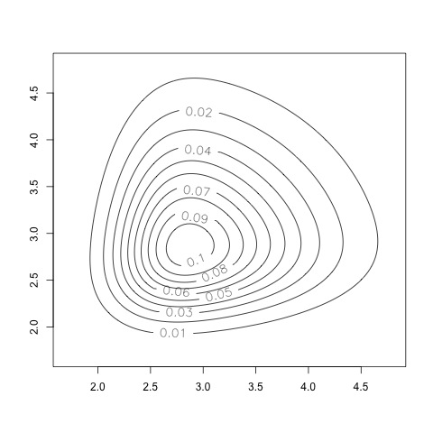
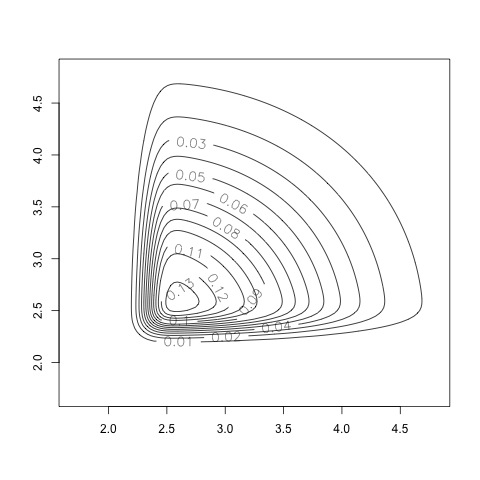
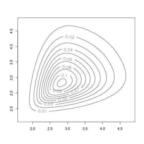
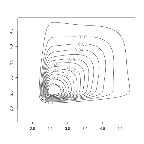
In Figure 2 we show plots of the bivariate wrapped skew normal distributions.

Figure 2: Bivariate densities of the wrapped skew normal with $\mu=\pi$, $\sigma^{2}=1$, $\lambda=3$ in the first column and $\lambda=10$ in the second column and several values of $\rho_{x}$ and $\rho_{w}$.

(a) $\rho_{x}=0.2$ and $\rho_{w}=0.2$

(b) $\rho_{x}=0.2$ and $\rho_{w}=0.2$

(c) $\rho_{x}=0.2$ and $\rho_{w}=0.8$

(d) $\rho_{x}=0.8$ and $\rho_{w}=0.2$

3 The wrapped skew Gaussian process

A natural way to construct a wrapped skew Gaussian process $\Theta(\mathbf{s}),\mathbf{s}\in\mathbb{R}^{d}$ is to start from a skew Gaussian process $Z(\mathbf{s})$ on the line and define, for each $\mathbf{s}$, $\Theta(\mathbf{s})=Z(\mathbf{s})\mbox{ mod }2\pi$, following the approach of Jona Lasinio et al (2012). To capture stationarity we use the following stationary skew Gaussian process, proposed by Zhang and El-Shaarawi (2010):

$$Z(\mathbf{s})=\mu+\frac{\sigma\lambda}{\sqrt{1+\lambda^{2}}}|X(\mathbf{s})|+\frac{\sigma}{\sqrt{1+\lambda^{2}}}W(\mathbf{s})-\frac{\sigma\lambda\sqrt{2}}{\sqrt{\pi(1+\lambda^{2})}}.$$ (19)

Here, $X(\mathbf{s})$ and $W(\mathbf{s})$ are independent zero mean Gaussian process with isotropic parametric correlation functions, $\boldsymbol{\rho}_{x}(h;\boldsymbol{\psi}_{x})$ and $\boldsymbol{\rho}_{w}(h;\boldsymbol{\psi}_{w})$, respectively.

The process in (19) is not the only stationary skew Gaussian process proposed in the literature. However, Minozzo and Ferracuti (2012) point out that most of them are in fact not stationary. For example Kim and Mallick (2004) or Allard and Naveau (2007) built stochastic skew normal processes where the $n-$finite dimensional distributions have, as special case, the multivariate skew normal of Azzalini and Capitanio (1999). But, the class of multivariate skew normal of Azzalini and Capitanio (1999) is not closed under marginalization. Each marginal is still a skew normal but not of the same form, and Minozzo and Ferracuti (2012) demonstrate that the stationarity property of an $n-$dimensional finite distribution in this case is not passed onto the marginals. Note that if in (19) we let the process $X(\mathbf{s})$ to be spatially constant, i.e. $X(\mathbf{s})\equiv X$, the associated $n-$finite dimensional distributions are the Azzalini and Capitanio (1999)’s multivariate skew normal and then, from above, the process is not stationary. On the other hand, if the process $W(\mathbf{s})$ is spatially constant, it is easy to demonstrate that (19) can be written as

$$Z(\mathbf{s})=\mu+\frac{\sigma\lambda}{\sqrt{1+\lambda^{2}}}|X^{*}(\mathbf{s})|-\frac{\sigma\lambda\sqrt{2}}{\sqrt{\pi(1+\lambda^{2})}},$$ (20)

where $X^{*}(\mathbf{s})$ is a process with finite dimensional distributions that are a mixture of folded normal with mode at $\mathbf{0}$ and covariance matrix that depends on the covariance matrix of $X(\mathbf{s})$ and on the parameters $\sigma^{2}$ and $\lambda$. As a consequence the resulting process is not a skew Gaussian process.

The correlation in each of the $X(\mathbf{s})$ and $W(\mathbf{s})$ processes induces association for the $\Theta(\mathbf{s})$ process. However, because circular variables have no magnitude (they only acquire a numerical value given an orientation), there is no unique way to define the correlation between two circular variables $\Theta(\mathbf{s})$ and $\Theta(\mathbf{s}^{\prime})$. A common choice, which exhibits most of the desirable properties of a correlation, is the one proposed by Jammalamadaka and Sarma (1988), that is,

$$\frac{E[\cos(\Theta(\mathbf{s})-\Theta(\mathbf{s}^{\prime})|\boldsymbol{\Psi})-\cos(\Theta(\mathbf{s})+\Theta(\mathbf{s}^{\prime})+2\tilde{\mu}|\boldsymbol{\Psi})]}{2\sqrt{E(\sin^{2}(\Theta(\mathbf{s})-\tilde{\mu})|\boldsymbol{\Psi})E(\sin^{2}(\Theta(\mathbf{s}^{\prime})-\tilde{\mu})|\boldsymbol{\Psi})}}.$$ (21)

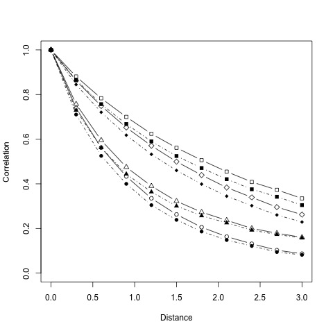
In our setting (21) is not a valid correlation function; it is not a positive definite function. Moreover, we cannot compute (21) in closed form but, again, we can resort to Monte Carlo approximation. Figure 3 provides an illustrative display of the inline and corresponding circular correlations arising from the exponential correlation functions $\boldsymbol{\rho}_{x}(h;\boldsymbol{\psi}_{x})=\exp(-h\psi_{x})$ and $\boldsymbol{\rho}_{w}(h;\boldsymbol{\psi}_{w})=\exp(-h\psi_{w})$.

Figure 3: Correlation functions for the inline (empty symbols) and circular (solid symbols) process with $\sigma^{2}=1$, $\delta=0.95$ and exponential correlation function for the processes $X(\mathbf{s})$ and $W(\mathbf{s})$ with respectively decays parameters 0.5 and 0.5 (circle), 0.5 and 0.2 (triangle), 0.2 and 0.5 (rhombus), 0.2 and 0.2 (square)

3.1 Implementation and Kriging

Working directly with the wrapped skew Gaussian process is not feasible since the likelihood for a $n-$dimensional realization of the circular process involves $n$ doubly infinite sums, i.e. let $\boldsymbol{\Theta}=(\Theta(\mathbf{s}_{1}),$ $\Theta(\mathbf{s}_{2}),\dots,\Theta(\mathbf{s}_{n}))^{\prime}$ and $\mathbf{K}=(K(\mathbf{s}_{1}),$ $K(\mathbf{s}_{2}),\dots,K(\mathbf{s}_{n}))^{\prime}$, the density of $\boldsymbol{\Theta}|\boldsymbol{\psi}$ is

$$f(\boldsymbol{\theta}|\boldsymbol{\Psi})=\sum_{k_{1}\in\mathbb{Z}}\sum_{k_{2}\in\mathbb{Z}}\dots\sum_{k_{n}\in\mathbb{Z}}g(\boldsymbol{\theta}+2\pi\mathbf{k}|\boldsymbol{\Psi}),$$ (22)

where $g(\cdot|\boldsymbol{\Psi})$ is the density of $\mathbf{Z}=\boldsymbol{\Theta}+2\pi\mathbf{K}$, the realization of the skew Gaussian process. When dealing with wrapped distributions the winding numbers are treated as latent random variables (see Jona Lasinio et al, 2012; Coles, 1998, for details and ideas). Hence, the joint distribution of the circular variables and the winding numbers coincides with the joint distribution of the associated linear variables, i.e., $g(\cdot|\boldsymbol{\Psi})$, and we can work directly with the process $Z(\mathbf{s})$.
A critical point is the following. To simplify the model fitting, recalling (10) and (11) and extending them to $n-$variate random variables, $\mathbf{Z}|\mathbf{X},\boldsymbol{\Psi}$ is normal, hence the process $Z(\mathbf{s})|X(\mathbf{s}),\boldsymbol{\Psi}$ is Gaussian and $\Theta(\mathbf{s})|X(\mathbf{s}),\boldsymbol{\Psi}$ is wrapped Gaussian. This implies that, in the model fitting, if we further introduce the realization of the latent Gaussian process, $X(\mathbf{s})$, along with the set of winding numbers, the $K(\mathbf{s}_{i})$s, then the MCMC implementation follows directly from the work of Jona Lasinio et al (2012) on the wrapped Gaussian process.
In this setting, kriging is straightforward. More precisely, let $\mathbf{s}_{0}$ be the spatial location where we want to predict the circular process and let $\mathbf{X}=(X(\mathbf{s}_{1}),X(\mathbf{s}_{2}),\dots,$ $X(\mathbf{s}_{n}))^{\prime}$. As is customary in the Bayesian framework, to perform kriging we draw samples from the predictive distribution of $\Theta(\mathbf{s}_{0})|\boldsymbol{\Theta}$:

$$f(\Theta(\mathbf{s}_{0})|\boldsymbol{\Theta})= \sum_{\mathbf{K}\in\mathbb{Z}^{n}}\int_{\boldsymbol{\Psi}}f(\Theta(\mathbf{s}_{0})|X(\mathbf{s}_{0}),\mathbf{X},\mathbf{K},\boldsymbol{\Psi},\boldsymbol{\Theta})\times$$ (23)

$$f(X(\mathbf{s}_{0})|\mathbf{X},\boldsymbol{\Psi})f(\mathbf{X},\mathbf{K},\boldsymbol{\Psi}|\boldsymbol{\Theta})d\boldsymbol{\Psi}.$$ (24)

Let $\boldsymbol{\Psi}^{b}$, $\mathbf{X}^{b}$ and $\mathbf{K}^{b}$ be the $b^{th}$ sample from the posterior distribution $f(\mathbf{X},\mathbf{K},\boldsymbol{\Psi}|\boldsymbol{\Theta})$. We can sample from (24) with composition sampling. That is, if for each posterior sample we simulate $X^{b}(\mathbf{s}_{0})$ from the distribution $X(\mathbf{s}_{0})|\mathbf{X}^{b},\boldsymbol{\Psi}^{b}$ and $\Theta^{b}(\mathbf{s}_{0})$ from the distribution $\Theta(\mathbf{s}_{0})|X^{b}(\mathbf{s}_{0}),$ $\mathbf{X}^{b},\mathbf{K}^{b},$ $\boldsymbol{\Psi}^{b},\boldsymbol{\Theta}$, then each $\Theta^{b}(\mathbf{s}_{0})$ can be considered as a sample from (24).
We can easily simulate $X^{b}(\mathbf{s}_{0})$ since $X(\mathbf{s}_{0}),\mathbf{X}^{b}|\boldsymbol{\Psi}^{b}$ is Gaussian and then $X(\mathbf{s}_{0})|\mathbf{X}^{b},\boldsymbol{\Psi}^{b}$ is univariate normal with mean and covariance that can be derived using standard results. If we simulate $Z^{b}(\mathbf{s}_{0})$ from $Z(\mathbf{s}_{0})|\mathbf{Z}^{b},$ $X^{b}(\mathbf{s}_{0}),\mathbf{X}^{b},\boldsymbol{\Psi}^{b}$, where $\mathbf{Z}^{b}=\boldsymbol{\Theta}+2\pi\mathbf{K}^{b}$, we can immediately obtain $\Theta^{b}(\mathbf{s}_{0})$ as $\Theta^{b}(\mathbf{s}_{0})=Z^{b}(\mathbf{s}_{0})\mbox{ mod }2\pi$, that is a sample from $\Theta(\mathbf{s}_{0})|X^{b}(\mathbf{s}_{0}),$ $\mathbf{X}^{b},\mathbf{K}^{b},\boldsymbol{\Psi}^{b},\boldsymbol{\Theta}$. Remark that to obtain a sample of $Z^{b}(\mathbf{s}_{0})$ is really easy since

$$\left(\begin{array}[]{c}Z(\mathbf{s}_{0})\\ \mathbf{Z}\end{array}\right)|\mathbf{X},X(\mathbf{s}_{0}),\boldsymbol{\Psi}\sim$$ (27)

$$N\left(\begin{array}[]{c}\mu^{*}+\frac{\sigma\lambda}{\sqrt{1+\lambda^{2}}}|X(\mathbf{s}_{0})|\\ \mu^{*}\mathbf{1}_{n}+\frac{\sigma\lambda}{\sqrt{1+\lambda^{2}}}|\mathbf{X}|\end{array},\frac{\sigma^{2}}{1+\lambda^{2}}\left(\begin{array}[]{cc}1&\boldsymbol{\rho}_{0,w}^{\prime}\\ \boldsymbol{\rho}_{0,w}&\mathbf{\Upsilon}\end{array}\right)\right)$$ (32)

where $\mathbf{1}_{n}$ is a vector of 1s of dimension $n$, $(\mathbf{\Upsilon})_{ij}=\rho_{w}(||\mathbf{s}_{i}-\mathbf{s}_{j}||;\boldsymbol{\psi}_{w})$ and $(\boldsymbol{\rho}_{0,w})_{i}=\rho_{w}(||\mathbf{s}_{i}-\mathbf{s}_{0}||;\boldsymbol{\psi}_{w})$. Then the distribution of $Z(\mathbf{s}_{0})|\mathbf{Z}^{b},X^{b}(\mathbf{s}_{0}),\mathbf{X}^{b},\boldsymbol{\Psi}^{b}$ is normal.

4 A dynamic extension of the wrapped skew Gaussian process

We extend our model to the dynamic setting following ideas in Banerjee et al (2014). We start by specifying an inline process $Z_{t}(\mathbf{s})$, $t\in[1,\dots,T]$, as

$$Z_{1}(\mathbf{s}) =\mu+\frac{\sigma\lambda}{\sqrt{1+\lambda^{2}}}|X_{1}(\mathbf{s})|$$ (33)

$$+\frac{\sigma}{\sqrt{1+\lambda^{2}}}W_{1}(\mathbf{s})-\frac{\sigma\lambda\sqrt{2}}{\sqrt{\pi(1+\lambda^{2})}},$$ (34)

$$Z_{t}(\mathbf{s}) =\mu+\gamma(Z_{t-1}(\mathbf{s})-\mu)+\frac{\sigma\lambda}{\sqrt{1+\lambda^{2}}}|X_{t}(\mathbf{s})|$$ (35)

$$+\frac{\sigma}{\sqrt{1+\lambda^{2}}}W_{t}(\mathbf{s})-\frac{\sigma\lambda\sqrt{2}}{\sqrt{\pi(1+\lambda^{2})}},\,t\neq 1,$$ (36)

where $\gamma\in[-1,1]$, $\forall t$ we have $X_{t}(\mathbf{s})|\boldsymbol{\Psi}\sim GP(0,\boldsymbol{\rho}_{x}(h;\boldsymbol{\psi}_{x}))$, $W_{t}(\mathbf{s})|\boldsymbol{\Psi}\sim GP(0,\boldsymbol{\rho}_{w}(h;\boldsymbol{\psi}_{w}))$ and $\mbox{Cov}(X_{t}(\mathbf{s}),X_{t^{\prime}}(\mathbf{s}^{\prime})|\boldsymbol{\Psi})=\mbox{Cov}(W_{t}(\mathbf{s}),W_{t^{\prime}}(\mathbf{s}^{\prime})|\boldsymbol{\Psi})=0$ if $t\neq t^{\prime}$. Expressions (34) and (36) provide a mean-centered, first order auto-regressive model with i.i.d. process increments. Moreover, the process increments are skew GP’s with parameters $\sigma,\lambda,\rho_{x},\rho_{w}$. Equivalently, we see that $Z_{1}(\mathbf{s})|\boldsymbol{\Psi}\sim SGP(\mu,\sigma^{2},\lambda)$ and $Z_{t}(\mathbf{s})|Z_{t-1}(\mathbf{s}),\boldsymbol{\Psi}\sim SGP(\mu+\gamma(Z_{t-1}(\mathbf{s})-\mu),\sigma^{2},\lambda)$.

Under the dynamic spatial setting, we are generally interested in predicting the process (i) at an observed spatial location at time $T+h$, $h\in\mathbb{Z}^{+}$ (usually $h=1$) or (ii) at an unobserved spatial location $\mathbf{s}_{0}$ inside the observed time window. Suppose we let $\mu^{b}$, $(\sigma^{2})^{b}$, $\lambda^{b}$ and $\gamma^{b}$ be the samples of the parameters of the $b^{th}$ iteration of the MCMC algorithm, $({\mu}^{*})^{b}=\mu^{b}-{\sigma^{b}\lambda^{b}\sqrt{2}}/{\sqrt{\pi(1+(\lambda^{b})^{2})}}$, $X_{t}^{b}(\mathbf{s})$ and $K_{t}^{b}(\mathbf{s})$ the $b^{th}$ realization of the processes $X_{t}(\mathbf{s})$ and $K_{t}(\mathbf{s})$ at site $\mathbf{s}$ and time $t$ and $Z_{t}^{b}(\mathbf{s})=X_{t}(\mathbf{s})+2\pi K_{t}^{b}(\mathbf{s})$. $B$ samples from the predictive distribution $\Theta_{T+h}(\mathbf{s})|\boldsymbol{\Theta}$, where $\boldsymbol{\Theta}$ is the observed circular data, can be obtained if, for each MCMC sample, we draw a value $Z_{T+h}^{b}(\mathbf{s})$ from a normal distribution with mean

$$({\mu}^{*})^{b}+(\gamma^{b})^{h}(Z_{T}^{b}(\mathbf{s})-\mu^{b})+\frac{\sigma^{b}\lambda^{b}}{\sqrt{1-(\lambda^{b})^{2}}}|X_{T+h}^{b}(\mathbf{s})|$$

and variance

$$\frac{(\sigma^{2})^{b}}{1-(\lambda^{b})^{2}}.$$

The set $\{\Theta_{T+1}^{b}(\mathbf{s})\}_{b=1}^{B}$ is from the desired predictive distribution.

To obtain the $b^{th}$ posterior sample of the predictive distribution of $\Theta_{t}(\mathbf{s}_{0})|\boldsymbol{\Theta}$ we adopt the usual composition sampling by first sampling $X_{t}^{b}(\mathbf{s}_{0})$ from the distribution of $X_{t}(\mathbf{s}_{0})|\mathbf{X},\boldsymbol{\Psi}^{b}$ and then sampling $Z_{t}^{b}(\mathbf{s}_{0})$ from $Z_{t}(\mathbf{s}_{0})|\mathbf{Z},\mathbf{X},X_{t}^{b}(\mathbf{s}_{0}),\boldsymbol{\Psi}^{b}$. Finally, $\Theta_{t}^{b}(\mathbf{s}_{0})=Z_{t}^{b}(\mathbf{s}_{0})\mbox{ mod }2\pi$ is a draw from the predictive distribution $\Theta_{t}(\mathbf{s}_{0})|\boldsymbol{\Theta}$.

The distribution of $Z_{t}(\mathbf{s}_{0}),\mathbf{Z}|\mathbf{X},X_{t}^{b}(\mathbf{s}_{0}),\boldsymbol{\Psi}^{b}$ is again multivariate normal and for spatial locations $\mathbf{s}_{i},i=1,2,...,n$, let $\mathbf{Z}_{t}=(Z_{t}(\mathbf{s}_{1}),Z_{t}(\mathbf{s}_{2}),\dots,Z_{t}(\mathbf{s}_{n}))^{\prime}$, $\mathbf{Z}=(\mathbf{Z}_{1},\mathbf{Z}_{2},\dots,\mathbf{Z}_{T})^{\prime}$ and $\mathbf{X}$ be the associated realization of the process $X(\mathbf{s})$. Let $\boldsymbol{\Gamma}$ be a $T\times T$ correlation matrix with $i,j$th element equal to $\gamma^{|i-j|}$, $\boldsymbol{\Gamma}_{l}$ be the lower triangular part of $\boldsymbol{\Gamma}$ and $\mathbf{C}$ be the correlation matrix of $\mathbf{W}_{t}=(W_{t}(\mathbf{s}_{1}),W_{t}(\mathbf{s}_{2}),\dots,W_{t}(\mathbf{s}_{n}))^{\prime}$. Let $\mathbf{D}$ be a vector of length $n$ with $i^{th}$ element equal to $\mbox{Cor}(W_{t}(\mathbf{s}_{0}),W(\mathbf{s}_{i}))$, $\mathbf{F}_{t}$ be a vector of length $T$ with $i^{th}$ element equal to $\gamma^{|t-i|}$, $\mathbf{I}_{n}$ be the identity matrix of dimension $n$ and let $\otimes$ indicates the Kronecker product. Altogether, we have that

$$\left(\begin{array}[]{c}Z_{t}(\mathbf{s}_{0})\\ \mathbf{Z}\end{array}\right)|\mathbf{X},X_{t}(\mathbf{s}_{0}),\boldsymbol{\Psi}\sim$$ (39)

$$N\left(\begin{array}[]{c}{\mu}^{*}+\frac{\sigma\lambda}{\sqrt{1-\lambda^{2}}}|X_{t}(\mathbf{s}_{0})|\\ \boldsymbol{\delta}\end{array},\frac{\sigma^{2}}{1-\lambda^{2}}\left(\begin{array}[]{cc}1&(\mathbf{F}_{t}\otimes\mathbf{D})^{\prime}\\ \mathbf{F}_{t}\otimes\mathbf{D}&\boldsymbol{\Gamma}\otimes\mathbf{C}\end{array}\right)\right)$$ (44)

where

$$\boldsymbol{\delta}=\mu\mathbf{1}_{nT} +{\sigma\lambda}/{\sqrt{1-\lambda^{2}}}\left(\boldsymbol{\Gamma}_{l}\otimes\mathbf{I}_{n}\right)|\mathbf{X}|$$ (45)

$$-{\sigma\lambda\sqrt{2}}/{\sqrt{\pi(1+\lambda^{2})}}\left(\boldsymbol{\Gamma}_{l}\otimes\mathbf{I}_{n}\right)\mathbf{1}_{nT}.$$ (46)

Here, again $Z_{t}(\mathbf{s}_{0})|\mathbf{Z},\mathbf{X},X_{t}^{b}(\mathbf{s}_{0}),\boldsymbol{\Psi}^{b}$ is univariate normal and sampling from it is easy.

5 A brief simulation study

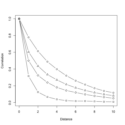
We fit and estimate the model proposed in Section 4 to 8 datasets simulated with $\mu=\pi$, $\sigma^{2}=1$ and 4 levels of the skew parameter $\lambda=\{0.0,1.5,3,10\}$. For the AR(1) parameter we chose $\gamma=0.5$; we experimented with several values of $\gamma\in(0,1)$ obtaining similar results, so we report estimates using the central value of the interval. We work with 2 sample sizes, 110 spatial locations and 60 time points, ($N=n\times T=110\times 60$), 220 spatial locations and 60 time points, $N=220\times 60$), to assess whether there are differences in the parameter estimates when the sample size increases. The coordinates are uniformly generated over $[0,10]^{2}$ and for both processes, $X_{t}(\mathbf{s})$ and $W_{t}(\mathbf{s})$, we adopt exponential correlation functions. We choose $\psi_{x}=0.5$ and $\psi_{w}=0.2$ and notice that, as $\lambda$ varies, we obtain different spatial correlations as shown in Figure 4.

Figure 4: Spatial correlation functions for the simulated datasets: circles are associated to Data1 ($\lambda=0$), triangles to Data2 ($\lambda=1.5$), diamonds to Data3 ($\lambda=3$) and squares to Data4 ($\lambda=10$).

The model is estimated with 90% of the spatial locations, i.e. 100 for the first sample size and 200 for the second, using the first 50 time points. Therefore, the training set is made of $100\times 50$ and $200\times 50$ points. We select observations using simple random sampling on the spatial locations (probability of inclusion in the training set $1/n$). The remaining spatial locations and 10 final time points are used to define two types of validation sets: (i) prediction at observed times, i.e. we use observations between time 1 and time 50 not used to estimate the models. To simplify we call this set the spatial validation set; (ii) prediction at unobserved times, i.e. we use observations from time 51 to time 60 at spatial locations used to estimate the models. We call this set the temporal validation set. We repeat the sampling procedure 40 times.

As prior distributions we use $\mu\sim U(0,2\pi)$, $\gamma\sim U(-1,1)$, $\psi_{x}\sim U(0.1,1)$ and $\psi_{w}\sim U(0.1,1)$. To choose the prior on $\sigma^{2}$ and $\lambda$ we note that, as for the wrapped Normal case (Jona Lasinio et al, 2012), if the variance of the associated inline distribution increases we are unable to tell the difference between the wrapped skew normal and a circular uniform. As we noted in Section 2.1, the variance of the skew normal is

$${\sigma^{2}\lambda^{2}}/{({1+\lambda^{2}})}\left(1-{2}/{\pi}\right)+{\sigma^{2}}/{({1+\lambda^{2}})},$$

i.e., it is a function of both $\sigma^{2}$ and $\lambda$. In this regard, when $\sigma^{2}=10$, with sample size of 200, independently of $\lambda$, the Rayleigh test of (circular) uniformity fails to discriminate between the wrapped skew normal and the circular uniform. So, we chose $\sigma^{2}\sim U(0,10)$ and a weak informative prior for $\lambda$, $\lambda\sim N(0,100)$.

$n=110$
Data1 ($\lambda=0$) Data2 ($\lambda=1.5$) Data3 ($\lambda=3$) Data4 ($\lambda=10$) $\hat{\mu}$ 3.03 3.365 3.217 3.109 C.I. (2.762 3.321) (3.205 3.533) (3.106 3.334) (3.044 3.177) $\hat{\sigma}^{2}$ 1.715 1.213 1.061 0.962 C.I. (1.390 2.186) (1.080 1.388) (0.976 1.177) (0.888 1.046) $\hat{\lambda}$ 0.931 1.690 3.278 9.864 C.I. (0.689 1.275) (1.498 1.924) (2.881 3.716) (8.572 11.282) $\hat{\gamma}$ 0.388 0.446 0.499 0.488 C.I. (0.35 0.42) (0.421 0.470) (0.479 0.518) (0.475 0.502) $\hat{\psi}_{x}$ 0.234 0.399 0.472 0.528 C.I. (0.139 0.483) (0.332 0.473) (0.413 0.528) (0.475 0.589) $\hat{\psi}_{w}$ 0.144 0.254 0.191 0.210 C.I. (0.109 0.186) (0.195 0.318) (0.141 0.251) (0.137 0.307)
$n=220$
Data1 ($\lambda=0$) Data2 ($\lambda=1.5$) Data3 ($\lambda=3$) Data4 ($\lambda=10$) $\hat{\mu}$ 2.981 3.353 3.209 3.094 C.I. (2.713 3.261) (3.209 3.504) (3.067 3.346) (3.031 3.161) $\hat{\sigma}^{2}$ 1.448 1.087 1.097 0.956 C.I. (1.266 1.701) (0.994 1.196) (1.005 1.211) (0.887 1.034) $\hat{\lambda}$ -0.716 1.383 2.501 9.619 C.I. (-0.869 -0.589) (1.242 1.532) (2.227 2.777) (8.449 10.771) $\hat{\gamma}$ 0.370 0.436 0.488 0.499 C.I. (0.349 0.390) (0.418 0.452) (0.474 0.503) (0.490 0.507) $\hat{\psi}_{x}$ 0.430 0.558 0.500 0.511 C.I. (0.323 0.625) (0.485 0.639) (0.444 0.558) (0.467 0.555) $\hat{\psi}_{w}$ 0.152 0.286 0.192 0.152 C.I. (0.119 0.186) (0.235 0.340) (0.143 0.245) (0.112 0.212)

Table 1: Parameter estimates (mean) and credible intervals (C.I.) for the wrapped skew Gaussian model in the 4 simulated datasets

$n=110$
Data1 ($\lambda=0$) Data2 ($\lambda=1.5$) Data3 ($\lambda=3$) Data4 ($\lambda=10$) $\hat{\mu}$ 2.986 3.313 3.208 3.138 C.I. (2.752 3.222) (3.211 3.409) (3.123 3.290) (3.082 3.199) $\hat{\sigma}^{2}$ 1.141 0.596 0.465 0.369 C.I. (0.993 1.340) (0.556 0.645) (0.438 0.497) (0.35 0.39) $\hat{\gamma}$ 0.415 0.417 0.489 0.488 C.I. (0.388 0.441) (0.392 0.441) (0.465 0.514) (0.463 0.514) $\hat{\psi}_{w}$ 0.225 0.67 0.796 1.182 C.I. (0.189 0.261) (0.611 0.726) (0.731 0.862) (1.099 1.265)
$n=220$
Data1 ($\lambda=0$) Data2 ($\lambda=1.5$) Data3 ($\lambda=3$) Data4 ($\lambda=10$) $\hat{\mu}$ 3.023 3.308 3.181 3.143 C.I. (2.833 3.210) (3.216 3.403) (3.103 3.254) (3.090 3.205) $\hat{\sigma}^{2}$ 1.061 0.602 0.473 0.370 C.I. (0.937 1.209) (0.564 0.647) (0.449 0.501) (0.354 0.390) $\hat{\gamma}$ 0.365 0.426 0.468 0.503 C.I. (0.346 0.384) (0.407 0.444) (0.452 0.487) (0.486 0.519) $\hat{\psi}_{w}$ 0.273 0.678 0.867 1.152 C.I. (0.237 0.309) (0.626 0.730) (0.809 0.923) (1.081 1.218)

Table 2: Parameter estimates (mean) and credible intervals (C.I.) for the wrapped Gaussian model in the 4 simulated datasets

For each dataset we also fit a wrapped normal model (setting $\lambda=0$) and we compare the models with regard to posterior point estimates and predictive ability. The predictive ability of the models is evaluated by computing the continuous rank probability score (CRPS) for circular variables (Grimit et al, 2006). The CRPS is a proper scoring rules defined, for circular variables, as

$$CRPS(F,\xi)=E(d(\Xi,\xi))-\frac{1}{2}E(d(\Xi,\Xi^{*})),$$ (47)

where $F$ is the predictive distribution, $\xi$ is the holdout value, $\Xi$ and $\Xi^{*}$ are independent copies of a circular variable with distribution $F$, and $d(\Xi,\Xi^{*})=1-{\cos}(\Xi-\Xi^{*})$, the circular distance (Jammalamadaka and SenGupta, 2001, p. 15). Exact calculation of (47) is not possible since we can not obtain the predictive distribution under the skew or the non skew Gaussian process in closed form. However, for the validation point $\theta_{t}(\mathbf{s}_{0})$ we can compute a Monte Carlo approximation as

$$\frac{1}{B}\sum_{b=1}^{B}d(\theta_{t}^{b}(\mathbf{s}_{0}),\theta_{t}(\mathbf{s}_{0}))-\frac{1}{2B^{2}}\sum_{l=1}^{B}\sum_{b=1}^{B}d(\theta_{t}^{l}(\mathbf{s}_{0}),\theta_{t}^{b}(\mathbf{s}_{0}))$$ (48)

where $\theta_{t}^{b}(\mathbf{s}_{0})$ denotes the simulated value of $\theta_{t}(\mathbf{s}_{0})$ using the $b^{th}$ posterior parameters and $B$ is the total number of posterior samples.

Figure 5: Illustrative predictive distributions for a holdout site in the first (a) and in the fourth simulated dataset (b). The solid line is the predictive distribution under the wrapped Gaussian model while the dashed one is under the wrapped skew Gaussian model. The vertical line represents the true holdout simulated value

(a) Data1

(b) Data4

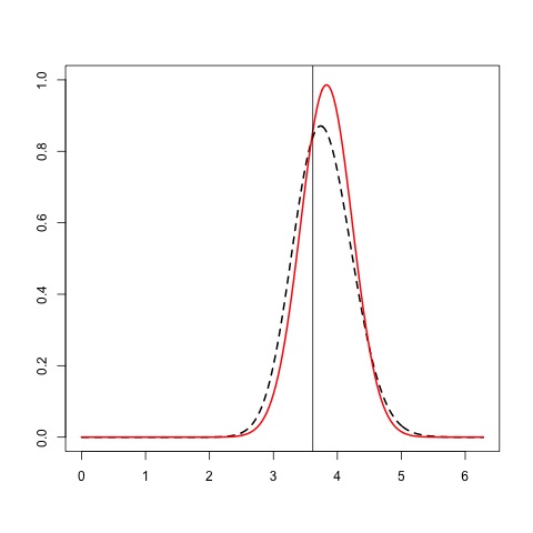
As an example, in Tables 1 and 2 we present the posterior mean estimates and credible intervals for all the parameters in all simulated datasets using one training set, i.e. the same locations and times for each dataset. For the fourth dataset and for both sample sizes, the skew model well estimates the parameters (the true value is inside the credible interval (C.I.)). In the first dataset $\lambda$ is far from 0. The wrapped skew normal process shows a substantial gain relative to the wrapped Gaussian process in terms of predictive ability for locations inside the observed time windows, even if the true model used to simulate the data is the wrapped Gaussian (Data1), see Table 3. As for forecasting (temporal validation set), we see that there is no difference between the models in terms of CPRS. Illustrative comparison of the predictive distributions under the two models can be seen in Figure 5. As we expect,in the fourth dataset the predictive distribution is highly skewed while, in the first, it is essentially symmetric.

Spatial
Data1 Data2 Data3 Data4 n=110 WS 0.173 0.146 0.118 0.116 W 0.221 0.179 0.176 0.160 n=220 WS 0.170 0.149 0.116 0.091 W 0.205 0.179 0.168 0.148
Temporal
Data1 Data2 Data3 Data4 n=110 WS 0.348 0.266 0.188 0.181 W 0.349 0.265 0.191 0.184 n=220 WS 0.350 0.275 0.193 0.181 W 0.349 0.272 0.194 0.183

Table 3: Simulated datasets: mean CRPSs over 40 validation sets. Models based on the wrapped skew normal (WS) and the wrapped normal (W)

6 The wave direction data example

	calm	calm	storm	storm
	WS	W	WS	W
$\hat{\mu}$	3.372	3.19	3.398	3.39
C.I.	(2.610 4.150)	(2.905 3.500)	(2.498 4.274)	(2.939 3.851)
$\hat{\sigma}^{2}$	5.246	1.827	5.015	1.283
C.I.	(4.214 6.883)	(1.526 2.276)	(4.029 6.581)	(1.130 1.477)
$\hat{\lambda}$	1.432	$\cdot$	1.159	$\cdot$
C.I.	(1.068 1.762)	($\cdot$ $\cdot$)	(0.868 1.496)	($\cdot$ $\cdot$)
$\hat{\gamma}$	0.438	0.567	0.377	0.479
C.I.	(0.406 0.471)	(0.540 0.594)	(0.350 0.406)	(0.453 0.504)
$\hat{\psi}_{x}$	0.006	$\cdot$	0.006	$\cdot$
C.I.	(0.005 0.008)	($\cdot$ $\cdot$)	(0.005 0.008)	($\cdot$ $\cdot$)
$\hat{\psi}_{w}$	0.002	0.013	0.001	0.007
C.I.	(0.001 0.003)	(0.011 0.015)	(0.001 0.001)	(0.005 0.008)

Table 4: Parameter estimates (mean) and credible intervals (C.I.) for the wave direction data

The real data we use come from a deterministic wave model implemented by Istituto Superiore per la Protezione e la Ricerca Ambientale (ISPRA) that gives hourly prediction over a grid of about 12.5$\times$12.5 Km on the Adriatic sea (Speranza et al, 2004). Over the Adriatic Sea area, there are 1494 points, with minimum and maximum distance of about 7km and 852km respectively. The computer model starts from a wind forecast model predicting the surface wind over the entire Mediterranean and then the prediction of the wave direction is obtained solving energy transport equations using the wind forecast as input.

We developed two datasets. The first spans the period April 2010 between the 2nd at 00:00 and the 4th at 22:00, a calm period. The second spans the period April 2010 between the 5th at 00:00 and the 7th at 22:00, a storm period. We randomly select 220 spatial locations; the same spatial locations are used for the calm and storm period dataset.

Similarly to what we did in the simulated examples, we use 90% of the spatial locations, taking the first 48 time points to estimate models while the remaining locations and times are included in the building of the two types of validation sets.

Again, for each training set, we fitted a skew Gaussian model and a wrapped Gaussian model. We repeat the splitting procedure into training and validation sets 40 times and each time we compute the CRPS to compare the performance of the models.
As prior distributions we used the same choices as in Section 5 with the exception of the spatial decays; for $\psi_{w}$ we adopt a $U(10^{-3},10^{-1})$ which corresponds to a maximum and minimum practical range of 3000km and 30km while for $\psi_{x}$ we adopt a $U(5^{-4},5^{-2})$ which roughly corresponds to the same practical spatial range for the process $|X(\mathbf{s})|$.

	calm	calm	storm	storm
	WS	W	WS	W
Spatial	0.426	0.494	0.528	0.567
Temporal	0.520	0.628	0.446	0.476

Table 5: Wave data: mean CRPSs over 40 validation sets. Models based on the wrapped skew normal (WS) and the wrapped normal (W)

In Table 4 we provide the parameters estimates for the first selected training sets. The estimated spatial dependence ($\psi_{w}$) of the $W(\mathbf{s})$ process is stronger during the storm for both models while ($\psi_{x}$) seems to remain the same in both sea states for $X(\mathbf{s})$. Again, employing the CRPS, for both validation sets under both sea states, the wrapped skew Gaussian process shows a consequential gain in predictive ability compared with the standard wrapped Gaussian.
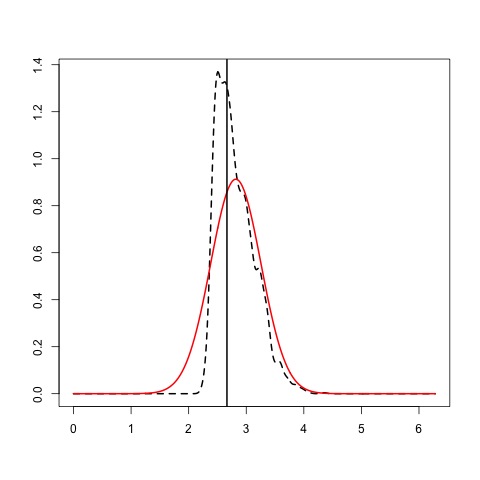
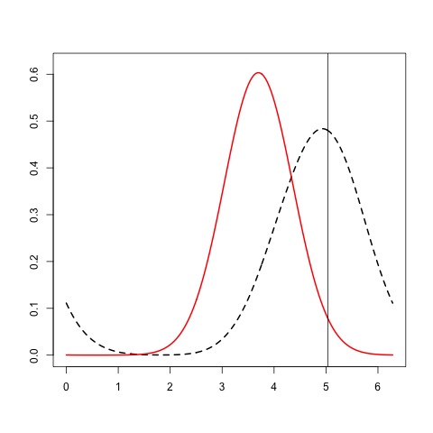
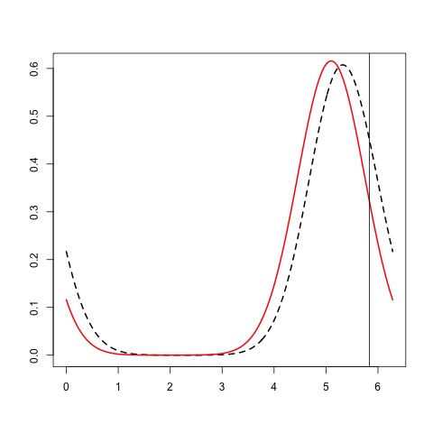
Finally, Figure 6 shows examples of predictive distributions for a holdout sample during a calm and a storm state. We showed in Figure 1 that with $|\lambda|<3$ there is little difference between the (symmetric) wrapped normal and the (asymmetric) wrapped skew normal. Since, in these two examples $|\hat{\lambda}|<1.5$, the predictive distributions under the skew normal models are roughly symmetric.

Figure 6: Examples of predictive distributions for one of the holdout site in calm (a) and storm (b) sea state. The solid line is the predictive distribution under the wrapped Gaussian model while the dashed one is under the skew Gaussian model. The vertical line represents the true holdout observed value

(a) Calm

(b) Storm

7 Summary and future work

We have presented a novel process model for dynamic spatial directional data. That is, we have a conceptual time series of directions at each spatial location in the region and we observe these series for a finite collection of locations. The model, referred to as a wrapped skew Gaussian process, enables more flexible marginal distributions for the locations than the symmetric ones that are available under the previously published wrapped Gaussian process. Using both simulation and a wave direction dataset, we are able to show improved out-of-sample prediction with the former.

Future work offers several opportunities. One is to note that wave heights are available in addition to wave directions. Wave heights inform about the sea state and therefore whether we are in a calm, storm, or transition state. In particular, predictive uncertainty varies with wave height and/or sea state, e.g., prediction is more precise during storm. So, we can attempt to extend the proposed model to introduce covariates into the mean model and also into the variance model for the wrapped skew Gaussian process. Another possibility is to model temporal data, where the time of the observed event is treated as random. Then, upon wrapping, we would have circular times. In addition, the locations of the events are random. The data would be treated as a point pattern over space and (circular) time.

References

- Allard and Naveau (2007) Allard D, Naveau P (2007) A new spatial skew-normal random field model. Communications in Statistics - Theory and Methods 36(9):1821–1834
- Azzalini (1985) Azzalini A (1985) A class of distributions which includes the normal ones. Scandinavian Journal of Statistics 12:171–178
- Azzalini (2005) Azzalini A (2005) The skew-normal distribution and related multivariate families. Scandinavian Journal of Statistics 32(2):159–188
- Azzalini and Capitanio (1999) Azzalini A, Capitanio A (1999) Statistical applications of the multivariate skew normal distribution. Journal of the Royal Statistical Society Series B (Statistical Methodology) 61(3):pp. 579–602
- Azzalini and Valle (1996) Azzalini A, Valle AD (1996) The multivariate skew-normal distribution. Biometrika 83(4):715–726
- Banerjee et al (2014) Banerjee S, Gelfand AE, Carlin BP (2014) Hierarchical modeling and analysis for spatial data, 2nd edn. Chapman and Hall/CRC, New York
- Bao et al (2009) Bao L, Gneiting T, Grimit EP, Guttorp P, Raftery AE (2009) Bias correction and bayesian model averaging for ensemble forecasts of surface wind direction. Monthly Weather Review 138(5):1811–1821
- Breckling (1989) Breckling J (1989) The analysis of directional time series: applications to wind speed and direction. Lecture notes in statistics, Springer-Verlag, Berlin Heidelberg
- Coles (1998) Coles S (1998) Inference for circular distributions and processes. Statistics and Computing 8(2):105–113
- Coles and Casson (1998) Coles S, Casson E (1998) Extreme value modelling of hurricane wind speeds. Structural Safety 20(3):283 – 296
- Damien and Walker (1999) Damien P, Walker S (1999) A full Bayesian analysis of circular data using the von Mises distribution. The Canadian Journal of Statistics 27:291–298
- Engel and Ebert (2007) Engel C, Ebert E (2007) Performance of hourly operational consensus forecasts (ocfs) in the australian region. Weather and Forecasting 22(6):1345–1359
- Fisher and Lee (1994) Fisher N, Lee A (1994) Time series analysis of circular data. Journal of the Royal Statistical Society: Series B (Statistical Methodology) 56:327:332
- Fisher (1996) Fisher NI (1996) Statistical analysis of circular data. Cambridge University Press, Cambridge
- Fisher and Lee (1992) Fisher NI, Lee AJ (1992) Regression models for an angular response. Biometrics 48(3):665–677
- Grimit et al (2006) Grimit EP, Gneiting T, Berrocal VJ, Johnson NA (2006) The continuous ranked probability score for circular variables and its application to mesoscale forecast ensemble verification. Quarterly Journal of the Royal Meteorological Society 132(621C):2925–2942
- Guttorp and Lockhart (1988) Guttorp P, Lockhart RA (1988) Finding the location of a signal: A bayesian analysis. Journal of the American Statistical Association 83(402):322–330
- Harrison and Kanji (1988) Harrison D, Kanji GK (1988) The development of analysis of variance for circular data. Journal of Applied Statistics 15:197–224
- Hernández-Sánchez and Scarpa (2012) Hernández-Sánchez E, Scarpa B (2012) A wrapped flexible generalized skew-normal model for a bimodal circular distribution of wind direction. Chilean Journal of Statistics 3(2):129–141
- Holzmann et al (2006) Holzmann H, Munk A, Suster M, Zucchini W (2006) Hidden Markov models for circular and linear-circular time series. Environmental and Ecological Statistics 13(3):325–347
- Hughes (2007) Hughes G (2007) Multivariate and time series models for circular data with applications to protein conformational angles. PhD thesis, University of Leeds, Leeds, UK
- Jammalamadaka and Sarma (1988) Jammalamadaka S, Sarma Y (1988) A correlation coefficient for angular variables. Statistical Theory and Data Analysis II pp 349–364
- Jammalamadaka and SenGupta (2001) Jammalamadaka SR, SenGupta A (2001) Topics in circular statistics. World Scientific, Singapore
- Jona Lasinio et al (2012) Jona Lasinio G, Gelfand A, Jona Lasinio M (2012) Spatial analysis of wave direction data using wrapped Gaussian processes. Annals of Applied Statistics 6(4):1478–1498
- Kato (2010) Kato S (2010) A Markov Process for Circular Data. Journal of the Royal Statistical Society: Series B (Statistical Methodology) 72(5):655–672
- Kato and Shimizu (2008) Kato S, Shimizu K (2008) Dependent models for observations which include angular ones. Journal of Statistical Planning and Inference 138(11):3538–3549
- Kato et al (2008) Kato S, Shimizu K, Shieh GS (2008) A circular-circular regression model. Statistica Sinica 18:633–645
- Kim and Mallick (2004) Kim HM, Mallick BK (2004) A Bayesian prediction using the skew gaussian distribution. Journal of Statistical Planning and Inference 120(1â2):85 – 101
- Lagona et al (2015) Lagona F, Picone M, Maruotti A, Cosoli S (2015) A hidden Markov approach to the analysis of space-time environmental data with linear and circular components. Stochastic Environmental Research and Risk Assessment 29(2):397–409
- Ma and Genton (2004) Ma Y, Genton MG (2004) A flexible class of skew-symmetric distributions. Scandinavian Journal of Statistics pp 459–468
- Mardia (1972) Mardia KV (1972) Statistics of directional data. Academic Press, London and New York
- Mardia and Jupp (1999) Mardia KV, Jupp PE (1999) Directional statistics. John Wiley and Sons, Chichcster
- Mastrantonio et al (2015) Mastrantonio G, Jona Lasinio G, Gelfand AE (2015) Spatio-temporal circular models with non-separable covariance structure. TEST To appear
- Minozzo and Ferracuti (2012) Minozzo M, Ferracuti L (2012) On the existence of some skew-normal stationary process. Chilean Journal of Statistics 3(2):157–170
- Nuñez-Antonio and Gutiérrez-Peña (2005) Nuñez-Antonio G, Gutiérrez-Peña E (2005) A Bayesian analysis of directional data using the projected normal distribution. Journal of Applied Statistics 32(10):995–1001
- Pewsey (2000) Pewsey A (2000) The wrapped skew-normal distribution on the circle. Communications in Statistics - Theory and Methods 29(11):2459–2472
- Pewsey (2006) Pewsey A (2006) Modelling asymmetrically distributed circular data using the wrapped skew-normal distribution. Environmental and Ecological Statistics 13(3):257–269
- Presnell et al (1998) Presnell B, Morrison SP, Littell RC (1998) Projected multivariate linear models for directional data. Journal of the American Statistical Association 93(443):1068–1077
- Ravindran and Ghosh (2011) Ravindran P, Ghosh SK (2011) Bayesian analysis of circular data using wrapped distributions. Journal of Statistical Theory and Practice 5(4):547–561
- Sahu et al (2003) Sahu SK, Dey DK, Branco MD (2003) A new class of multivariate skew distributions with applications to bayesian regression models. Canadian Journal of Statistics 31(2):129–150
- Speranza et al (2004) Speranza A, Accadia C, Casaioli M, Mariani S, Monacelli G, Inghilesi R, Tartaglione N, Ruti PM, Carillo A, Bargagli A, Pisacane G, Valentinotti F, Lavagnini A (2004) Poseidon: An integrated system for analysis and forecast of hydrological, meteorological and surface marine fields in the Mediterranean area. Nuovo Cimento 27(C):329–345
- Wang and Gelfand (2013) Wang F, Gelfand AE (2013) Directional data analysis under the general projected normal distribution. Statistical Methodology 10(1):113–127
- Wang and Gelfand (2014) Wang F, Gelfand AE (2014) Modeling space and space-time directional data using projected Gaussian processes. Journal of the American Statistical Association 109(508):1565–1580
- Wang et al (2004) Wang J, Boyer J, Genton MG (2004) A skew-symmetric representation of multivariate distributions. Statistica Sinica 14:1259–1270
- Zhang and El-Shaarawi (2010) Zhang H, El-Shaarawi A (2010) On spatial skew-Gaussian processes and applications. Environmetrics 21(1):33–47
- Zhang et al (2010) Zhang Q, Snow Jones A, Rijmen F, Ip EH (2010) Multivariate discrete hidden Markov models for domain-based measurements and assessment of risk factors in child development. Journal of Computational and Graphical Statistics 19(3):746–765