Equilibration of energy in slow-fast systems
Abstract
Ergodicity is a fundamental requirement for a dynamical system to reach a state of statistical equilibrium. On the other hand, it is known that in slow-fast systems ergodicity of the fast sub-system impedes the equilibration of the whole system due to the presence of adiabatic invariants. Here, we show that the violation of ergodicity in the fast dynamics effectively drives the whole system to equilibrium. To demonstrate this principle we investigate dynamics of the so-called springy billiards. These consist of a point particle of a small mass which bounces elastically in a billiard where one of the walls can move - the wall is of a finite mass and is attached to a spring. We propose a random process model for the slow wall dynamics and perform numerical experiments with the springy billiards themselves and the model. The experiments show that for such systems equilibration is always achieved; yet, in the adiabatic limit, the system equilibrates with a positive exponential rate only when the fast particle dynamics has more than one ergodic component for certain wall positions.
I Introduction
In classical statistical mechanics, one deals with systems of a large number of degrees of freedom, where the exact knowledge of the state of the system at any given moment of time is impossible or irrelevant. One, therefore, declares the state variables “microscopic” and tries to describe the statistics of “macroscopic” variables (certain functions of the microscopic state) in an ensemble of many systems similar to the given one. In other words, statistical mechanics examines averaging over the phase space of a dynamical system, typically a Hamiltonian one. There is no a priori way of choosing the probability distribution over which the averaging is performed: given a dynamical system, its evolution is different for different initial conditions, and the distribution of the initial conditions is not encoded in the system and can be arbitrary. However, one notices that the microscopic variables are usually changing fast, so the observed macroscopic quantities are, in fact, time averages. If the system is ergodic with respect to the Liouville measure (the uniform measure in the phase space restricted to a given energy level), then the Birkhoff ergodic theorem allows one to replace time averaging by averaging with respect to the Liouville measure. In other words, ergodicity dictates that the averaging must be universally performed over the micro-canonical ensemble Huang ; Reif ; Dorfman . After this choice of the ensemble is made, standard results of statistical mechanics are recovered (e.g. for a system of a large number of weakly coupled systems, each of which has a bounded energy, the averaging over the Liouville measure in the phase space of the full system yields the canonical Gibbs distribution of the energies of the constituent systems Hil14 ).
The main problem is that Hamiltonian systems are usually not ergodic, even if the number of degrees of freedom is large. For example, the gas of hard spheres is, most probably, ergodic Sinai1979 ; Simanyi1999 , but replacing the collisions of the spheres by mutual repulsion will, quite probably, ruin the ergodicity, even for an arbitrarily steep repulsing force potential Rapoport2006 ; Kaplan2001 . In general, the picture of dynamics in a smooth potential appears to be of a chaotic sea (a hyperbolic set in the phase space) with stability islands (regions in the phase space that contain a positive measure set filled by KAM-tori) Zas85 ; lict92 . When the islands occupy a noticeable portion of the phase space, the use of the micro-canonical ensemble for averaging is unfounded. This problem can be lifted by postulating (as, for example, an experimental fact) that the systems of physical interest are sufficiently close to ergodicity (the islands are small).
However, such universal “apparent ergodicity” postulate contains an intrinsic flaw. Indeed, consider an isolated system with a few slow degrees of freedom, the rest being fast. Would the fast subsystem be universally ergodic, the evolution of slow variables would obey adiabatic laws. In this case the full system would have a conserved quantity other than the energy - the Gibbs volume entropy of the fast subsystem as a function of the slow variables (one can view the slow variables as parameters of the fast system that change adiabatically, and adiabatic processes are known to keep the entropy constant Hil14 ). One has to have significant fluctuations in the fast subsystem in order to destroy this additional conserved quantity, otherwise the full slow-fast system will not appear ergodic on a long time scale. A rigorous formulation of this fact is given by Anosov-Kasuga averaging theorem AnosovKasuga . A celebrated example of the ergodicity in the fast subsystem preventing the equilibration in the full system is the “notorious piston problem”: it immediately follows from the adiabatic compression law that the system of two ideal gases at different temperatures contained in a finite cylinder and separated by an adiabatic movable piston never comes to equilibrium, which seems to defy the second law of thermodynamics LebPiSi00 ; Lieb99 ; Neishtadt2004 ; Wright2007 .
In this paper we resolve this issue by proposing a general mechanism for the onset of an apparent phase space ergodicity and mixing in slow-fast Hamiltonian systems. It is not based on the assumption of a large number of degrees of freedom, nor on the inherent instability of dispersing geometries (such as the hard spheres models). Instead, we assume that the fast subsystem is not ergodic for a significant range of values of the slow variables. We call such systems multi-component, as the fast subsystem has several ergodic components on its energy level. For simplicity, we also assume that for some values of the slow variables the fast subsystem is ergodic (i.e., has only one ergodic component). We demonstrate that in this case slow observables converge exponentially to the vicinity of their averages with respect to the Liouville measure for the full system. This suggests, somewhat paradoxically, that the non-ergodic behaviour of the fast degrees of freedom leads to equilibration of the full system.
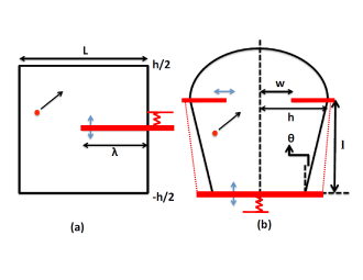
To elucidate this principle we construct a specific realization of slow-fast systems - the springy billiard models. This is a point particle of a small mass which bounces elastically in a billiard in which one of the walls, hereafter called the bar, can move. The bar is heavy (has mass and is attached to a spring, so, typically, the bar motion is slow and the particle motion is fast.
When the mass ratio vanishes, the bar motion is independent of the particle dynamics and the particle gains or loses speed at the collisions with the bar without changing the periodic motion of the bar. This process is studied under the name of Fermi acceleration Lichtenberg1980 ; Jarz1993 ; Lieberman1998 ; Loskutov2000 ; Cohen2003 ; Leonel2006 ; Lenz2008 ; Dolgopyat2008 ; Itin2012 ; Shah2010 ; Shah2011 ; Gelfreich2011 ; Gelfreich2012 ; Gelfreich2014 ; Batistic2014 ; Shah2015 ; Pereira2015 ; Turaev2016 . It has been established that there are two types of Fermi acceleration. If the frozen billiard is ergodic for all possible positions of the bar (ergodic accelerators), then the ensemble averaged kinetic energy may grow at most quadratically in time Loskutov2000 ; Leonel2006 ; Gelfreich2011 ; Gelfreich2012 . If the ergodicity of the frozen billiard is broken for a part of the period of the bar motion (a multi-component accelerator), then the particle kinetic energy growth is exponential in time for almost every initial condition Gelfreich2011 ; Shah2010 ; Shah2011 ; Shah2015 ; Batistic2014 ; Gelfreich2014 ; Pereira2015 . Figure 1 presents the billiard tables we consider here, including both ergodic (stadium) and multi-component (rectangle with a bar, mushroom) accelerators.
In the finite mass case (), the particle energy must remain bounded for all time, and the question of acceleration is replaced by the question of equilibration - will the kinetic energies of the particle and the moving bar equilibrate? The numerics we perform always show exponential equilibration, however there is a sharp difference between the ergodic and multi-component cases. The equilibration time within the ergodic accelerator tends to infinity as , while it stays bounded in the multi-component case.
We analyze this effect by deriving a model for the slow bar motion where the force exerted on the bar by the particle is found by averaging over one of the ergodic components. In the multi-component case, the change in the slow variables (the bar position) drives the fast system (the particle in the instantaneous billiard) to switch between different ergodic components. Assuming that the switching is well approximated by a Markov process, we derive the switching probabilities and construct a stochastic model for the bar motion (with no adaptable parameters). We verify the model by numerically comparing its behavior with the behavior of the corresponding springy billiards at small . As expected, in the ergodic case the model for the slow bar motion has a conserved quantity, so the equilibration in the corresponding springy billiard occurs only due to fluctuations from the averaged motion, which explains the slowing down of the equilibration as the separation of time scales increases. In the multi-component case, the Markov process of hopping between the ergodic components leads to equilibration at positive rates. Numerics shows that the bar motion is quite accurately represented by this model and the equilibration rates remain non-zero and get close to the model Markov process rates as .
The derivation of stochastic model is not billiard specific. A similar Markov process can be constructed for an arbitrary slow-fast system with a non-ergodic fast subsystem, cf. Pereira2015 . Under standard irreducibility and aperiodicity conditions, such a process should converge to a unique stationary measure, and by uniqueness this must correspond to the Liouville measure of the full system. Therefore, we believe the proposed apparent ergodisation mechanism should be universally applicable.
II A Particle in a springy billiard
Consider a mass particle in a -dimensional billiard. One of the billiard walls, the bar of mass , is suspended on a spring with a spring constant , so it may oscillate vertically. At impact, the bar and the particle undergo an elastic collision leading to the exchange of momentum and energy between the bar and the particle:
where , and , are the vertical velocities of the bar and the particle just before and just after the collision. The total energy of the system is preserved, whereas the particle energy (hereafter denotes the particle velocity) and the bar energy ( is the bar position) change at impact.
The system “bar-particle” is a slow-fast degrees of freedom Hamiltonian system: is of order one whereas the particle speed is typically large (). Usually, when the particle moves sufficiently fast, many collisions with the bar occur in short time intervals, so the averaged motion of the bar is governed by the equation
| (1) |
where is the spring potential, and denotes the averaged force exerted on the bar at position by the particle with the energy . The averaging is performed over many collisions at a frozen value of . Since the work done by this force corresponds to the change in the particle’s energy, we conclude that .
If the frozen billiard is ergodic for each value of , then the Anosov-Kasuga theorem AnosovKasuga ; Jarz1993 ; Neishtadt2004 ; Wright2007 ; Gelfreich2012 implies that the phase space volume under a given energy level is approximately preserved (for most trajectories, for sufficiently small and on any finite interval of the slow time), hence
| (2) |
where is the volume of the billiard domain. This implies that the average force acting on the bar equals to . Note that the same formula follows from the ideal gas law. Since , Eq. 1 becomes
| (3) |
One may check that the bar motion defined by Eq. 3 indeed follows the level sets of . By noting that the adiabatic law of Eq. 2 takes the form , we find that the adiabatic bar motion is governed by an effective potential
| (4) |
where is determined by the initial condition. Similar effective potential was derived in the context of the piston problem Neishtadt2004 ; Wright2007 . It is easy to see that . Here corresponds to the pressure equilibrium, where the pressure due to the collisions with the particle is compensated by the force exerted by the spring ( depends on the total energy ). At the other extreme of , the particle does not move and all the energy is in the oscillating bar.
We performed numerical studies for a classical example of ergodic billiard - the slanted half-stadium BuniStad , with the springy oscillating bar at the bottom, see Fig. 1b with . When the initial speed of the particle in the stadium is large enough, we observe that the bar motion indeed follows a level line of for many bar oscillations. Since for all possible values of and the motion in the potential given by Eq. 4 is periodic, as long as the adiabatic invariant stays nearly constant the full system does not equilibrate. Notably, we demonstrate numerically that the motion for does lead to equilibration on a sufficiently long time scale. We also note that in accordance with the adiabatic theory, the numerically found equilibration time tends to infinity as (see the next section and Fig. 4).
Next, we present two multi-component springy billiards, in which the ergodicity of the fast dynamics is broken for some intervals of time. The first is the Rectangle with Oscillating Bar (ROB) Shah2010 , Fig. 1a. A particle moves in a rectangle (of length and height ) which is partially split by a length horizontal bar attached to a spring. The particle horizontal speed is preserved, so the horizontal motion is periodic with period . This period is divided into two time intervals. On the first one, the particle does not hit the bar and its vertical speed is preserved. On the second interval, of length , where , the particle enters a chamber above or below the bar where it gains or lose vertical speed as it hits the moving bar many times. Consequently, during a single passage above or below the bar, the vertical speed obeys the adiabatic law given by Eq. 2 with , and when the particle is above the bar and similarly, when below, (here do not include the particle horizontal kinetic energy which is decoupled from the dynamics). Hence . We further assume that the deterministic process is well approximated by a stochastic one, by which the probabilities to enter the chamber above/below the bar are proportional to the length of the gap between the bar and the upper or, respectively, lower boundary of the rectangle, i.e., these probabilities are equal to where is taken at the moment of entrance to the chamber. The same assumptions were used in Shah2010 for the study of Fermi acceleration in ROB in the case of infinitely heavy bar (the limit ); as numerics performed in Shah2010 show, these assumptions hold in the case with a good precision.
Since , the right-hand side of Eq. 1 becomes for particles above/below the bar, respectively. Hence, we suggest that the bar-particle system is well approximated by the following -periodic probabilistic hybrid system:
| (5) |
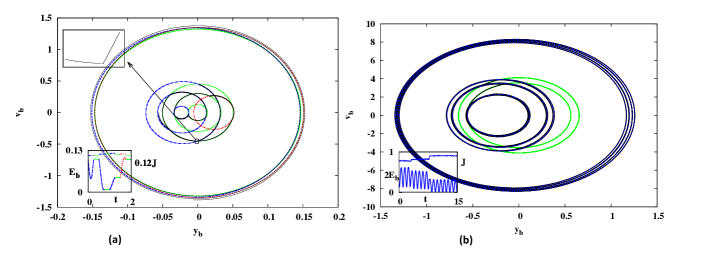
, , and . Namely, the bar dynamics follows the level lines of , , or . At , the bar height determines the probability to choose vs. , and determine the particular level set along which the motion will continue. Fig. 2a demonstrates that the bar motion of the springy ROB follows the level sets of the corresponding ’s. In the next section, we examine equilibration, demonstrating that at small the stochastic model given by Eq. 5 provides a good approximation to bar dynamics in the springy ROB billiard.
The ROB model represents a family of multicomponent billiards in which the transition from a single ergodic component to two (or more) possible ergodic components and back to a single component occurs at discrete sequence of prescribed times (e.g. at in the ROB model). Similar behavior occurs when one splits and unites -dimensional chaotic billiards by a moving wall (see Gelfreich2011 ; Gelfreich2012 ). In particular, for such systems the standard adiabatic law applies at each interval of time along which the particle motion corresponds to a single ergodic component, and a stochastic process similar to Eq. 5 provides a good model for the bar dynamics.
Next, we describe a different multi-component system, the slanted springy mushroom of Fig. 1b Gelfreich2014 ; BuniMush , in which particles leak from one ergodic component to another during some time interval. This is expected to be the generic behavior in systems with mixed phase space (see also Batistic2014 ; Pereira2015 ). The base of the mushroom stem is a springy bar with vertical position , so the mushroom stem length is . The mushroom throat width , which controls the capture and release of particles from the mushroom cap, changes in synchrony with the bar position as prescribed later on. This is a multi-component system - the motion is mixing in the stem and integrable in the cap BuniMush . The oscillations in lead to the exchange of particles between the integrable and chaotic zones Gelfreich2014 . In such situation, by which a particle in the chaotic component may leak into a different component at any instant of time in some time interval, the usual adiabatic law needs to be modified to the “leaky adiabatic law”:
| (6) |
(see Gelfreich2014 for derivation and corroboration for ). Here, is the total phase space volume for the frozen mushroom billiard on the energy level and is the phase space volume of the chaotic zone on the same energy level. Then (see details in Gelfreich2014 ) where This leaky adiabatic law implies that as long as the particle remains in the chaotic component the system has an adiabatic invariant given by where Hence, while the particle is not captured in the cap, the bar motion occurs along the level lines of producing an effective potential: where . When the elliptic zone is expanding , the particle may transfer from the chaotic to the elliptic zone. Since the motion in the stem is chaotic, we model the capture time as a random variable. We set the probability to transfer at the time interval from the stem to the cap as the ratio of the transferred phase space volume to the chaotic zone volume (see Gelfreich2014 ):
| (7) |
Once captured in the cap, the particle does not influence the bar, so the bar and particle energies are preserved separately and the bar moves only due to the spring force. The particle gets released from the cap at the time interval where is the first instance at which the throat reached back the width it had at the time of capture: and in the adiabatic limit vanishes. If is not a single-valued function of , the bar position is changed between the capture and the release time: , so after the capture episode the particle follows a new level set of . To ensure that is not single valued function of for all oscillations of the bar, we choose a protocol for the dependence of on for which takes its minimum at (recall that is the pressure equilibrium point where takes its maximal value, here ):
| (8) |
Hence, the stochastic model for the bar motion becomes
| (9) |
where the particle moves from the stem to the cap at time with probability given by Eq. 7, and subsequently gets released at (defined by ). Figure 2b demonstrates that the bar-particle simulations adhere to Eq. 9. We also verified that the distribution of capture events in the cap as a function of is well approximated by Eq. 7 and that the release time is well approximated by the equal throat-width rule. In the next section, we show that this stochastic model provides a good approximation to the equilibration process in the limit .
III Ensemble equilibration rates
So far, we have checked that the adiabatic theory, by which one averages the fast particle motion, enables to predict the evolution of the averaged bar motion for a finite time in each of the ergodic components of the fast system. In the case where the fast subsystem is ergodic, the predicted adiabatic bar motion is periodic, so no equilibration occurs as long as the adiabatic invariant is preserved. In the multi-component cases the bar motion follows effectively a random dynamical system by which the bar motion switches between different laws of motion, leading to chaotization of orbits, and hence equilibration.
To test equilibration, we examine the behavior of ensemble average of kinetic energies. By Equipatition Theorem, at equilibrium, the kinetic energy for each degree of freedom should be the same Hil14 . We thus define for the ROB and for the slanted stadium and mushroom.
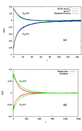
Numerically, we find that for finite , in all cases, for all initial ensembles, , see Fig. 3. This suggests that for finite the system gets close to equilibrium in finite time for both ergodic and multi-component springy billiards.
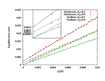
Next, we examine the equilibration rates. We find that the convergence to the equilibrium is exponential, yet the rate of convergence depends on the initial ensemble and, also, on the choice of the interval of fitting. Hereafter, in order to make a comparison between the rates of convergence in different models possible, we fix a practical definition of the equilibration rate as the best fitted slope to vs. on the time interval wher is defined by . For each fixed ensemble of initial conditions we examine how such defined rate depend on the mass ratio. For the ROB case the rates do not display any significant dependence on (see Fig. 3a). For the mushroom and stadium cases, the equilibration rates increase from their limit values proportionally to . By extrapolation to , we find that the limit equilibration rates for the stadium vanish (Fig. 4a) whereas for the mushroom they are positive (Fig. 4b).
This is our main finding, as it reveals the profound difference between the ergodic and multi-components cases. The vanishing of the equilibration rates in the ergodic case is in agreement with adiabatic theory. The positive rates achieved in the multi-component case reflect the efficient mixing induced by the hoping between the ergodic components.
The extrapolation of the data obtained by the simulations at non-zero can be sensitive to noise and the chice of the fitting procedure. Therefore, to claim that the limit equilibration rates are strictly positive in the multi-component cases, we need to benchmark them against their theoretical values. To this aim, we also simulate the stochastic models given by Eqs. 5 and 9, and observe that these models also equilibrate in a similar fashion, with the ensemble-dependent exponential rates close to those obtained by the springy billiard simulations at small (Fig. 4). Thus, we compare the ROB rates for initial ensembles with and , computed for 10 runs of 6000 particles each. The stochastic simulations of Eq. 5 produce the rates for the ensembles with the initial and for the ensembles with the initial , whereas the actual springy billiard simulations produce the rates, respectively, and for and and for . Similarly, the rates for the stochastic simulations of the mushroom model given by Eq. 9, computed for 10 runs of 10000 particles each, are whereas the limit values from Fig. 4b are and for and , respectively.
We conclude that the stochastic models, with no adaptable parameters, provide a reasonable approximation to the dynamics observed in our numerical experiments. These results support our claim that the behavior of slow-fast systems with a multi-component fast subsystem can be modeled by the random process of Markov switching between several different equations for slow evolution obtained by averaging over different ergodic components in the fast phase space.
IV Discussion
Springy billiards demonstrate an important principle in slow-fast Hamiltonian systems: ergodicity of the fast subsystem impedes the ergodisation in the full slow-fast system whereas its violation can lead to equilibration. Indeed, we computed the equilibration rates for ergodic and multi-component springy billiards and demonstrated, by extrapolation to , that the equilibration rates for the ergodic cases vanish in the limit whereas for the multi-component ones they are positive (Fig. 4). We showed that the limit behavior of the multi-component case is well approximated by a random process in which the slow variables follow the averaged dynamics on each ergodic component of the fast system, and switch randomly between these different averaged systems, leading to complete chaotization. We stress that in this random model of multi-component system both the magnitude and probabilities of the jumps remain finite as , hence the chaotization time remains bounded in this limit.
The observed sensitivity of the equilibration rates to the initial ensemble energy may be related to the two non-trivial regimes at (the Fermi acceleration limit) and (the pressure equilibrium). In both limits there is no exchange of energy between the slow and fast systems. Spectral properties of the operator governing the evolution of the densities are affected by these states.
The Fermi acceleration limit may be studied directly by taking an ensemble of fast particles with vanishing kinetic energy (e.g. ), so that initially the particles hardly influence the bar motion. Such particles accelerate exponentially fast in multi-component accelerators whereas in ergodic accelerators they accelerate as a power-law in time. This leads to distinct dependence of the transient time on : for a multi-component springy billiard the transients are of order whereas for an ergodic springy billiard they are much longer, of order .
Slower particles may resonate and possibly freeze, and this singular behavior may have non-trivial effects on the equilibration EckY10 . Such a behavior breaks the slow-fast structure and thus it cannot be treated by the stochastic model we propose. However, since this phase space region has small volume, its influence on the statistical behavior seems to be negligible.
We also propose that springy billiards may be used to study additional dynamical phenomena in slow-fast systems. First, in this paper we assumed for simplicity that the fast system is ergodic for a range of the slow variables and that this range is realized in every cycle of the slow system. In particular, in our setup, the pressure equilibrium points were always destabilized (in the springy mushroom case this motivated the choice of , see Eq. 8). Springy multi-component billiards for which this property is violated are easy to construct, and thus proper conditions under which such systems still lead to ergodization need to be formulated and studied. Such cases were considered in the Fermi acceleration limit for billiards Batistic2014 and for smooth homogeneous Hamiltonians Pereira2015 . Second, we considered a one degree of freedom slow system with a single fixed point which is always stable (a single bar moving vertically). Thus, the dynamics in each of the averaged slow systems is trivially integrable and periodic. More complicated situations, possibly with several degrees of freedom may be studied. Third, extended simulations and analysis of the random models may shed light on the role of islands and the effect of the singular regimes (the Fermi limit and the pressure equilibria). Fourth, incorporating the finite fluctuations into the random models is a challenging problem, for both the ergodic and multi-component cases.
The multi-component equilibration mechanism in springy billiards is expected to appear also in smooth slow-fast multi-component systems. In fact, the new chaotization mechanism we propose is reminiscent of the phenomena of adiabatic chaos - chaotization of smooth slow-fast systems in which the fast dynamics is integrable, yet the structure of the fast phase space changes as the slow variables are changed Tennyson1986 ; Vain1998 ; Neish1991 . The new suggestion here is that this mechanism is universal and is not restricted to fast subsystems that are integrable. In fact, if some of the ergodic components of the fast system are chaotic, and, moreover, if there exists a range of slow variables for which the chaotic ergodic component occupies a large portion of the fast subsystem phase space the equilibration may be particularly fast.
Finally, we propose a broader viewpoint on this work. Here, our slow and fast systems were just two mechanical components and the time-scale separation stemmed from the mass ratio. In the broader statistical mechanics context, the fast system governs the motion of many particles (and is thus high-dimensional) and the slow macroscopic variables are defined as certain averages over the fast, microscopic system. When the structure of the fast system changes, for example, from a gas to a liquid state, one declares that a phase transition occurs. Usually, for macroscopic values near phase transition, the microscopic phase space structure is complex, with long-lasting structures in which the two states coexist. We may say that in this range of the macroscopic variables the fast system is inherently multi-component. Therefore, we conjecture that phase transitions may play a central role in the equilibration process between microscopic and macroscopic variables (e.g. consider the analog of the notorious piston problem in a multi-phase gas).
Acknowledgement
RK acknowledges support by the Israel Science Foundation (grant 1208/16). KS and DT would like to acknowledge the financial support and hospitality of Weizmann Institute of Science where a part of this work was done. KS also thanks the SERB-DST, Government of India (File No. : SR/FTP/PS-108/2012) for financial support. DT acknowledges the support of RSF grant 14-41-00044 to this research, and also thanks the Royal Society and EPSRC. VG’s research was supported by EPRC (grant EP/J003948/1).
References
- (1) K. Huang (1987) Statistical mechanics (Wiley, New York).
- (2) F. Reif (1965) Fundamentals of statistical and thermal physics (McGraw Hill, New York).
- (3) J. R. Dorfman (2001) An introduction to chaos in nonequilibrium statistical mechanics (Cambridge University Press, Cambridge).
- (4) S. Hilbert, P. Hšanggi and J. Dunkel (2014) Thermodynamic laws in isolated systems. Phys. Rev. E 90:062116.
- (5) Ya. G. Sinai (1979) Ergodic properties of a Lorentz gas. Funct. Anal. Appl. 13:192.
- (6) N. Simanyi and D. Szasz (1999) Hard ball systems are completely hyperbolic. Annals of Mathematics 149:35.
- (7) A. Rapoport, V. Rom-Kedar and D. Turaev (2008) Stability in high dimensional steep repelling potentials. Comm. Math. Phys. 279:497-534.
- (8) A. Kaplan, N. Friedman, M. Andersen and N. Davidson (2001) Observation of Islands of Stability in Soft Wall Atom-Optics Billiards. Phys. Rev. Lett. 87:274101.
- (9) G. M. Zaslavsky (1985) Chaos in Dynamic Systems. (Harwood Academic, New York).
- (10) A. J. Lichtenberg and M.A. Lieberman (1992) Regular and Chaotic Dynamics (Springer-Verlag, New York).
- (11) D. V. Anosov (1960) Averaging in systems of ordinary differential equations with rapidly oscillating solutions. Izv. Akad. Nauk SSSR, Ser. Mat. 24:721 ; T. Kasuga (1961) On the adiabatic theorem for the Hamiltonian system of differential equations in the classical mechanics, I. Proc. Jpn. Acad. 37:366 ; P. Lochak and C. Meunier (1988) Multiphase averaging for classical systems (Springer-Verlag, New York).
- (12) E. H. Lieb (1999) Some problems in statistical mechanics that I would like to see solved. Physica A 263:491.
- (13) J. L. Lebowitz, J. Piasecki, and Ya. G. Sinai (2000) Scaling dynamics of a massive piston in an ideal gas. Hard ball systems and the Lorentz gas (Springer-Verlag, Berlin).
- (14) A. I. Neishtadt and Y. G. Sinai (2004) Adiabatic piston as a dynamical system. Journal of Statistical Physics 116:815.
- (15) P. Wright (2007) The periodic oscillation of an adiabatic piston in two or three dimensions. Commun. Math. Phys. 275:553.
- (16) A. J. Lichtenberg, M. A. Lieberman and R. H. Cohen (1980) Fermi acceleration revisited. Physica D 1:291.
- (17) C. Jarzynski (1993) Energy diffusion in a chaotic adiabatic billiard gas. Phys. Rev. E 48:4340.
- (18) M. A. Lieberman and V. A. Godyak (1998) From Fermi acceleration to collisionless discharge heating. IEEE Trans. Plasma Sci. 26:955.
- (19) A. Loskutov, A. B. Ryabov, and L. G. Akinshin (2000) Properties of some chaotic billiards with time-dependent boundaries. J. Phys. A 33:7973.
- (20) D. Cohen and D. A. Wisniacki (2003) Stadium billiard with moving walls. Phys. Rev. E 67:026206.
- (21) R. E. de Carvalho, F. C. Souza and E. D. Leonel (2006) Fermi acceleration on the annular billiard. Phys. Rev. E 73:066229.
- (22) F. Lenz, F. K. Diakonos and P. Schmelcher (2008) Tunable Fermi acceleration in the driven elliptical billiard. Phys. Rev. Lett. 100:014103.
- (23) D. Dolgopyat (2008) Fermi acceleration. Contemp. Math. 469:149.
- (24) A. P. Itin and A. I. Neishtadt (2012) Fermi acceleration in time-dependent rectangular billiards due to multiple passages through resonances. Chaos 22:026119.
- (25) K. Shah, D. Turaev and V. Rom-Kedar (2010) Exponential energy growth in a Fermi accelerator. Phys. Rev. E 81:056205.
- (26) K. Shah (2011) Energy growth rate in smoothly oscillating billiards. Phys. Rev. E 83:046215.
- (27) V. Gelfreich, V. Rom-Kedar, K.Shah and D. Turaev (2011) Robust exponential acceleration in time-dependent billiards. Phys. Rev. Lett. 106:074101.
- (28) V. Gelfreich, V. Rom-Kedar and D.Turaev (2012) Fermi acceleration and adiabatic invariants for non-autonomous billiards. Chaos 22:033116.
- (29) V. Gelfreich, V. Rom-Kedar and D. Turaev (2014) Oscillating mushrooms: Adiabatic theory for a non-ergodic system. J. Phys. A 47:395101. The collared stadium of Fig. 1b has the same phase space structure as the mushroom, yet one may change the collar width, , without moving additional walls.
- (30) B. Batistic (2014) Exponential Fermi acceleration in general time-dependent billiards. Phys. Rev. E 90:032909.
- (31) K. Shah, V. Gelfreich, V. Rom-Kedar and D. Turaev (2015) Leaky Fermi accelerators. Phys. Rev. E 91:062920.
- (32) T. Pereira and D. Turaev (2015) Exponential energy growth in adiabatically changing Hamiltonian systems. Phys. Rev. E 91:010901(R).
- (33) D. Turaev (2016) Exponential energy growth due to slow parameter oscillations in quantum mechanical systems. Phys. Rev. E 93:050203(R).
- (34) L. A. Bunimovich (1974) On ergodic properties of certain billiards. Funct. Anal. Appl. 8:254.
- (35) L. A. Bunimovich (2001) Mushrooms and other billiards with divided phase space. Chaos 11:802.
- (36) J.P. Eckmann and L.S. Young (2010) Rattling and freezing in a 1D transport model. Nonlinearity 24(1):207
- (37) J. L. Tennyson, J. R. Cary and D. F. Escande (1986) Change of the adiabatic invariant due to separatrix crossing. Phys. Rev. Lett. 56:2117.
- (38) D. L. Vainshtein, A. A. Vasiliev and A. I. Neishtadt (1998) Adiabatic chaos in a two-dimensional mapping. Chaos 6:514.
- (39) A. N. Neishtadt, D. K. Chaikovskii and A. A. Chernikov (1991) Adiabatic chaos and particle diffusion. Sov. Phys. JETP 72:423.