Interpretation of the new $\Omega_{c}^{0}$ states via their mass and width

Abstract

The mass and pole residue of the ground and first radially excited $\Omega_{c}^{0}$ states with spin-parities $J^{P}=1/2^{+},\,3/2^{+}$, as well as P-wave $\Omega_{c}^{0}$ with $J^{P}=1/2^{-},\,3/2^{-}$ are calculated by means of the two-point QCD sum rules. The strong decays of $\Omega_{c}^{0}$ baryons are also studied and width of these decay channels are computed. The relevant computations are performed in the context of the full QCD sum rules on the light-cone. Obtained results for the masses and widths are confronted with recent experimental data of LHCb Collaboration, which allow us to interpret $\Omega_{c}(3000)^{0}$, $\Omega_{c}(3050)^{0}$, and $\Omega_{c}(3119)^{0}$ as the excited $css$ baryons with the quantum numbers $(1P,\,1/2^{-})$, $(1P,\,3/2^{-})$, and $(2S,\,3/2^{+})$, respectively. The $(2S,\,1/2^{+})$ state can be assigned either to $\Omega_{c}(3066)^{0}$ state or $\Omega_{c}(3090)^{0}$ excited baryon.

I Introduction

The observation by the LHCb Collaboration of new narrow states $\Omega_{c}^{0}$ in the $\Xi_{c}^{+}K^{-}$ invariant mass distribution is one of the intriguing discoveries in physics of the heavy baryons LHCb . Preliminary analysis indicates that these five neutral resonances are composed of $css$ quarks, and may be orbitally/radially excited states of the $\Omega_{c}^{0}$ baryons with spins $1/2$ and $3/2$. Let us note, that till the LHCb data an experimental information about baryons with $css$ content was limited by the masses of the $\Omega_{c}^{0}$ and $\Omega_{c}(2770)^{0}$ particles Olive:2016xmw

$$m=2695.2\pm 1.7\,\mathrm{\,MeV},\,\,m=2765.9\pm 2.0\,\,\mathrm{MeV},$$ (1)

which were considered as the ground states with the spin-parities $J^{P}=1/2^{+}$ and $3/2^{+}$, respectively.

Theoretical investigations performed in the context of different approaches, and predictions obtained for the spectroscopic parameters provide incomparably more detailed information on the features of the $\Omega_{c}^{0}$ baryons, than experimental data Capstick:1986bm ; Bagan:1991sc ; Bagan:1992tp ; Chiladze:1997ev ; Huang:2000tn ; Wang:2002ts ; Ebert:2007nw ; Ebert:2011kk ; Garcilazo:2007eh ; Valcarce:2008dr ; Roberts:2007ni ; Wang:2007sqa ; Wang:2008hz ; Wang:2009cr ; Vijande:2012mk ; Yoshida:2015tia ; Edwards:2012fx ; Padmanath:2013bla ; Chen:2015kpa ; Chen:2016phw ; Shah:2016nxi ; Aliev:2015qea ; Azizi:2015ksa . In fact, the masses of the ground state and radially/orbitally excited heavy baryons including the $\Omega_{c}^{0}$ particles were calculated using the relativistic quark models Capstick:1986bm ; Ebert:2007nw ; Ebert:2011kk , the QCD sum rule method Bagan:1991sc ; Bagan:1992tp ; Huang:2000tn ; Wang:2002ts ; Wang:2007sqa ; Wang:2008hz ; Wang:2009cr ; Chen:2015kpa ; Chen:2016phw ; Aliev:2015qea ; Azizi:2015ksa , the Heavy Quark Effective Theory (HQET) Chiladze:1997ev , various quark models Garcilazo:2007eh ; Valcarce:2008dr ; Roberts:2007ni ; Vijande:2012mk ; Yoshida:2015tia ; Shah:2016nxi , and lattice simulations Edwards:2012fx ; Padmanath:2013bla . The strong couplings and transitions of the heavy flavored baryons, their magnetic moments and radiative decays also attracted interest of physicists Aliev:2015qea ; Azizi:2015ksa ; Zhu:1997as ; Aliev:2008sk ; Aliev:2009jt ; Aliev:2010nh ; Aliev:2010ev ; Aliev:2011kn ; Aliev:2011ufa ; Aliev:2011uf ; Aliev:2010ac . It is worth noting, that in some of these theoretical studies different assumptions were made on the structure of the heavy baryons. For example, in Refs. Ebert:2007nw ; Ebert:2011kk a heavy-quark-light-diquark picture were employed in the relativistic quark model. In other works, QCD sum rule calculations were carried out in the context of the HQET Huang:2000tn ; Wang:2002ts ; Chen:2015kpa ; Chen:2016phw .

The discovery of five new $\Omega_{c}^{0}$ particles by the LHCb Collaboration changed the existed experimental situation, and stimulated a theoretical activity to explain the observed states. These states were seen as resonances in the $\Xi_{c}^{+}K^{-}$ invariant mass distribution. Their masses do not differ considerably from each other and are within the range $M=3000-3150\,\mathrm{MeV}$. The transition $\Omega_{c}^{0}\to\Xi_{c}^{+}K^{-}$ may be considered as main decay modes of the $\Omega_{c}^{0}$ states, widths of which equal to a few $\mathrm{MeV}$.

The LHCb did not provide an information on the spin-parities of the new states, which is an important problem of ongoing theoretical investigations. Thus, in our Letter Agaev:2017jyt we have calculated the masses of the ground states and first radial excitations of $\Omega_{c}^{0}$ with $J^{P}=1/2^{+}$ and $3/2^{+}$, and found that the particles $\Omega_{c}(3066)$ and $\Omega_{c}(3119)$ can be considered as the radially excited $css$ baryons with the quantum numbers $(2S,\,1/2^{+})$ and $(2S,\,3/2^{+})$, respectively. In calculations we have employed the two-point QCD sum rule method by invoking into analysis general expressions for the currents to interpolate the $\Omega_{c}^{0}$ baryons with spins $1/2$ and $3/2$. Our results correctly describe the masses of the ground states $\Omega_{c}^{0}$ and $\Omega_{c}(2770)^{0}$, and agree with two of the recent experimental data of the LHCb Collaboration. It is interesting, that predictions obtained in some of previous theoretical studies agree with new LHCb data and our results (more detailed information can be found in Ref. Agaev:2017jyt , and in references therein), as well.

The problems connected with the $\Omega_{c}^{0}$ states have been addressed in Refs. Chen:2017sci ; Karliner:2017kfm ; Wang:2017vnc ; Padmanath:2017lng ; Yang:2017rpg ; Huang:2017dwn ; Kim:2017jpx ; Wang:2017hej ; Cheng:2017ove ; Wang:2017zjw ; Chen:2017 ; Zhao:2017 ; Aliev:2017led . The new particles have been assigned to be P-wave $\Omega_{c}$ baryons in Ref. Chen:2017sci , where the authors evaluated widths of their decay channels. Calculations there have been performed in the framework of HQET using the sum rule approach. In Refs. Karliner:2017kfm ; Wang:2017vnc $\Omega_{c}(3000)$, $\Omega_{c}(3050)$, $\Omega_{c}(3066)$, $\Omega_{c}(3090)$ and $\Omega_{c}(3119)$ have been interpreted as P-wave excited states of the $\Omega_{c}^{0}$ baryons with the spin-parities $1/2^{-},\,1/2^{-},\,3/2^{-},\,3/2^{-}$ and $5/2^{-}$, respectively. In Ref. Karliner:2017kfm an alternative set of assignments, namely $3/2^{-},\,3/2^{-},\,5/2^{-},\,1/2^{+}$ and $3/2^{+}$ is made for these states, as well. In this case $1/2^{-}$ states are expected around $2904$ and $2978$ $\mathrm{MeV}$. In both of Refs. Karliner:2017kfm ; Wang:2017vnc the authors utilized the heavy-quark-light-diquark model for $\Omega_{c}$ baryons. On the basis of lattice simulations the same conclusions have been made also in Ref. Padmanath:2017lng . Attempts have been done to classify new states as five-quark systems or S-wave pentaquark molecules with $J^{P}=1/2^{-},\,3/2^{-}$ and $5/2^{-}$ Yang:2017rpg ; Huang:2017dwn . The possible pentaquark interpretation of the $\Omega_{c}^{0}$ baryons on the basis of the quark-soliton model has been suggested also in Ref. Kim:2017jpx .

The explorations carried out in the context of a constituent quark model have allowed authors of Ref. Wang:2017hej to conclude, that $\Omega_{c}(3000)$ and $\Omega_{c}(3090)$ can be considered as states with $1/2^{-}$, $\Omega_{c}(3050)$ and $\Omega_{c}(3066)$ as the baryons with $3/2^{-}$ and $5/2^{-}$, whereas the $\Omega_{c}(3119)$ might correspond to one of the radial excitations $(2S,\,1/2^{+})$ or $(2S,\,3/2^{+})$. In Ref. Cheng:2017ove the first three states from the LHCb range of excited $\Omega_{c}$ baryons have been classified as P-wave states with $1/2^{-},\,5/2^{-}$ and $3/2^{-}$, whereas last two particles have been assigned to be $2S$ states with spin-parities $1/2^{+}$ and $3/2^{+}$, respectively. These states have been analyzed as the P-wave excitation of the $\Omega_{c}^{0}$ baryons with spin-parities $1/2^{-},\,1/2^{-},\,3/2^{-},\,3/2^{-}$ and $5/2^{-}$ also in Ref. Wang:2017zjw . The studies have been performed using the two-point sum rule method by introducing relevant interpolating currents.

The newly discovered $\Omega_{c}^{0}$ states, their spin-parities has been analyzed in Refs. Chen:2017 ; Zhao:2017 ; Aliev:2017led , too. Thus, studies in Ref. Chen:2017 showed that five resonances $\Omega_{c}^{0}$ can be grouped into the 1P states with negative parity, i.e. the resonances $\Omega_{c}(3000)$ and $\Omega_{c}(3090)$ have been considered there as $(1P,1/2^{-})$ states, $\Omega_{c}(3066)$ and $\Omega_{c}(3119)$ as resonances with $(1P,\,3/2^{-})$, and $\Omega_{c}(3050)$ as $(1P,\,5/2^{-})$ state. The alternative explanation has been suggested in Ref.  Zhao:2017 , where the resonances $\Omega_{c}(3066)$ and $\Omega_{c}(3090)$ have been interpreted as $1P$-wave states with the spin-parity $J^{P}=3/2^{-}$ or $J^{P}=5/2^{-}$. Starting from decay features of the remaining three resonances in Ref.  Zhao:2017 the authors have assigned them to be $1D$-wave $\Omega_{c}^{0}$ states. Finally, in Ref. Aliev:2017led the resonances $\Omega_{c}(3000)$ and $\Omega_{c}(3066)$ have been classified as the $(1P,\ 1/2^{-})$ and $(1P,\ 3/2^{-})$ states, respectively.

As is seen, a variety of suggestions made on the structures of the $\Omega_{c}^{0}$ states, methods and schemes used to compute their parameters, and obtained predictions for the spin-parities of these baryons is quite impressive. In the present work we are going to extend our previous paper by including into analysis P-wave $(1P,\,1/2^{-})$ and $(1P,\,3/2^{-})$ states, as well. We will evaluate the masses and pole residues of the ground and four excited $\Omega_{c}^{0}$ states. We will also calculate widths of $\Omega_{c}^{0}\rightarrow\Xi^{+}K^{-}$ decays using the light cone sum rule (LCSR) method, which is one of the powerful nonperturbative approaches to evaluate parameters of exclusive processes Balitsky:1989ry . Calculations will be performed by taking into account K meson’s distribution amplitudes (DAs). The extracted from analysis mass and decay width of $\Omega_{c}^{0}$ states will be confronted with existing LHCb data, and predictions obtained in theoretical papers. This will allows us to identify $\Omega_{c}(3000)$, $\Omega_{c}(3050)$, $\Omega_{c}(3066)$, and $\Omega_{c}(3119)$ by fixing their quantum numbers.

This work is structured in the following way. In Sec. II we calculate the mass and pole residue of the ground state and orbitally/radially excited $\Omega_{c}^{0}$ baryons with the quantum numbers $(1S,\,1/2^{+})\Rightarrow$ $\Omega_{c}$, $(1P,\,1/2^{-})\Rightarrow\Omega_{c}^{-}$, $(2S,\,1/2^{+})$ $\Rightarrow\Omega_{c}^{\prime}$, and $(1S,\,3/2^{+})\Rightarrow\Omega_{c}^{\star}$, $(1P,\,3/2^{-})\Rightarrow\Omega_{c}^{\star-}$, $(2S,\,3/2^{+})\Rightarrow\Omega_{c}^{\star\prime}$ . To this end, we employ the two-point sum rules method. In Sec. III we analyze $\Omega_{c}^{-}\Xi_{c}^{+}K^{-}$ and $\Omega_{c}^{\prime}\Xi_{c}^{+}K^{-}$ vertices to evaluate the corresponding strong couplings $g_{\Omega^{-}\Xi K}$ and $g_{\Omega^{\prime}\Xi K}$, and calculate widths of $\Omega_{c}^{-}\to\Xi_{c}^{+}K^{-}$ and $\Omega_{c}^{\prime}\to\Xi_{c}^{+}K^{-}$ decays. The similar investigations are carried out in Sec. IV for the vertices containing $\Omega_{c}^{0}$ baryons with $J^{P}=3/2^{+}$ and $J^{P}=3/2^{-}$. Here we find widths of the processes $\Omega_{c}^{\star-}\rightarrow\Xi_{c}^{+}K^{-}$ and $\Omega_{c}^{\star\prime}\rightarrow\Xi_{c}^{+}K^{-}$. In this section we also analyze the $\Omega_{c}^{\star\prime}\to\Xi_{c}^{\prime+}K^{-}$ decay, which is kinematically allowed only for $\Omega_{c}^{\star\prime}$ baryon. Section V is reserved for brief discussion of the obtained results. It contains also our concluding remarks. Explicit expressions of the correlation functions derived in the present work, as well as the quark propagators used in calculations are presented in Appendix.

II Masses and pole residues of the $\Omega_{c}^{0}$ states

In this section we evaluate the mass and pole residue of the spin $1/2$ and $3/2$ ground state and excited $\Omega_{c}$ (hereafter, we omit the superscript $0$ in $\Omega_{c}^{0}$) baryons by means of two-point sum rule method.

The sum rules necessary to find masses and residues of the $\Omega_{c}^{0}$ baryons can be derived using the two-point correlation function

$$\Pi_{(\mu\nu)}(p)=i\int d^{4}xe^{ipx}\langle 0|\mathcal{T}\{\eta_{(\mu)}(x)\overline{\eta}_{(\nu)}(0)\}|0\rangle,$$ (2)

where $\eta(x)$ and $\eta_{\mu}(x)$ are the interpolating currents for $\Omega_{c}$ states with spins $J=1/2$ and $J=3/2$, respectively. They have the following forms

$$\eta = -\frac{1}{2}\epsilon^{abc}\left\{\left(s^{aT}Cc^{b}\right)\gamma_{5}s^{c}+\beta\left(s^{aT}C\gamma_{5}c^{b}\right)s^{c}\right.$$ (3)

$$\left.-\left[\left(c^{aT}Cs^{b}\right)\gamma_{5}s^{c}+\beta\left(c^{aT}C\gamma_{5}s^{b}\right)s^{c}\right]\right\},$$

and

$$\eta_{\mu} = \frac{1}{\sqrt{3}}\epsilon^{abc}\left\{\left(s^{aT}C\gamma_{\mu}s^{b}\right)c^{c}+\left(s^{aT}C\gamma_{\mu}c^{b}\right)s^{c}\right.$$ (4)

$$\left.+\left(c^{aT}C\gamma_{\mu}s^{b}\right)s^{c}\right\}.$$

In expressions above $C$ is the charge conjugation operator. The current $\eta(x)$  for the $1/2$ baryons contains an arbitrary auxiliary parameter $\beta$, where $\beta=-1$ corresponds to the Ioffe current.

We start from the spin $1/2$ baryons and calculate the correlation function $\Pi^{\mathrm{Phys}}(p)$ in terms of the physical parameters of the states under consideration and determine $\Pi^{\mathrm{OPE}}(p)$ employing the quark propagators. Because, the current $\eta(x)$ couples not only to states $\Omega_{c}$ and $\Omega_{c}^{\prime}$, but also to $\Omega_{c}^{-}$, in the physical side of the sum rule we explicitly take into account their contributions by adopting the ”ground-state+first orbitally+first radially excited states+continuum” scheme: We follow an approach applied recently to calculate the masses and residues of radially excited octet and decuplet baryons in Refs. Aliev:2016jnp ; Aliev:2016adl . In these works the authors got results, which are compatible with existing experimental data on the masses of the radially excited baryons, and demonstrated that besides ground-state baryons the QCD sum rule method can be successfully applied to investigate their excitations, as well.

Thus, we find

$$\Pi^{\mathrm{Phys}}(p)=\frac{\langle 0|\eta|\Omega_{c}(p,s)\rangle\langle\Omega_{c}(p,s)|\overline{\eta}|0\rangle}{m^{2}-p^{2}}$$

$$+\frac{\langle 0|\eta|\Omega_{c}^{-}(p,\widetilde{s})\rangle\langle\Omega_{c}^{-}(p,\widetilde{s})|\overline{\eta}||0\rangle}{\widetilde{m}^{2}-p^{2}}$$

$$+\frac{\langle 0|\eta|\Omega_{c}^{\prime}(p,s^{\prime})\rangle\langle\Omega_{c}^{\prime}(p,s^{\prime})|\overline{\eta}||0\rangle}{m^{\prime 2}-p^{2}}+\ldots,$$ (5)

where $m$, $\widetilde{m}$, $m^{\prime}$ and $s$, $\widetilde{s}$, $s^{\prime}$ are the masses and spins of the $\Omega_{c}$, $\Omega_{c}^{-}$ and $\Omega_{c}^{\prime}$ baryons, respectively. The dots denote contributions of higher resonances and continuum states. In Eq. (5) the summations over the spins $s$, $\widetilde{s}$, $s^{\prime}$ are implied.

We proceed by introducing the matrix elements

$$\langle 0|\eta|\Omega_{c}^{(\prime)}(p,s^{(\prime)})\rangle=\lambda^{(\prime)}u^{(\prime)}(p,s^{(\prime)}),$$

$$\langle 0|\eta|\Omega_{c}^{-}(p,\widetilde{s})\rangle=\widetilde{\lambda}\gamma_{5}u^{-}(p,\widetilde{s}).$$ (6)

Here $\lambda$, $\widetilde{\lambda}$ and $\lambda^{\prime}$ are the pole residues of the $\Omega_{c}$, $\Omega_{c}^{-}$ and $\Omega_{c}^{\prime}$ states, respectively. Using Eqs. (5) and (6) and carrying out summation over spins of the $1/2$ baryons

$$\sum\limits_{s}u(p,s)\overline{u}(p,s)=\not{p}+m,$$ (7)

we obtain

$$\Pi^{\mathrm{Phys}}(p)=\frac{\lambda^{2}(\not{p}+m)}{m^{2}-p^{2}}+\frac{\widetilde{\lambda}^{2}(\not{p}-\widetilde{m})}{\widetilde{m}^{2}-p^{2}}$$

$$+\frac{\lambda^{\prime 2}(\not{p}+m^{\prime})}{m^{\prime 2}-p^{2}}+\ldots$$ (8)

The Borel transformation of this expression is:

$$\mathcal{B}\Pi^{\mathrm{Phys}}(p)=\lambda^{2}e^{-\frac{m^{2}}{M^{2}}}(\not{p}+m)$$

$$+\widetilde{\lambda}^{2}e^{-\frac{\widetilde{m}^{2}}{M^{2}}}(\not{p}-\widetilde{m})+\lambda^{\prime 2}e^{-\frac{m^{\prime 2}}{M^{2}}}(\not{p}+m^{\prime}).$$ (9)

As is seen, it contains the structures $\sim\not{p}$ and $\sim I$. In order to derive the sum rules we use both of them and find: from the terms $\sim\not{p}$

$$\lambda^{2}e^{-\frac{m^{2}}{M^{2}}}+\widetilde{\lambda}^{2}e^{-\frac{\widetilde{m}^{2}}{M^{2}}}+\lambda^{\prime 2}e^{-\frac{m^{\prime 2}}{M^{2}}}=\mathcal{B}\Pi_{1}^{\mathrm{OPE}}(p),$$ (10)

and from the terms $\sim I$

$$\lambda^{2}me^{-\frac{m^{2}}{M^{2}}}-\widetilde{\lambda}^{2}\widetilde{m}e^{-\frac{\widetilde{m}^{2}}{M^{2}}}+\lambda^{\prime 2}m^{\prime}e^{-\frac{m^{\prime 2}}{M^{2}}}=\mathcal{B}\Pi_{2}^{\mathrm{OPE}}(p),$$ (11)

where $\mathcal{B}\Pi_{1}^{\mathrm{OPE}}(p)$ and $\mathcal{B}\Pi_{2}^{\mathrm{OPE}}(p)$ are the Borel transformations of the same structures in $\Pi^{\mathrm{OPE}}(p)$ computed employing the quark propagators, as it has been explained above. It is assumed, that continuum contributions are subtracted from the right-hand sides of Eqs. (10) and (11) utilizing the quark-hadron duality assumption.

The derived sum rules contain six unknown parameters of the ground state and excited baryons. Therefore, from Eqs. (10) and (11) we determine the parameters $(m,\ \lambda)$ of the ground state $\Omega_{c}$ baryon by keeping there only the first terms, and choosing accordingly the continuum threshold parameter $s_{0}$ in $\Pi_{1}^{\mathrm{OPE}}(M^{2},\ s_{0})$ and $\Pi_{2}^{\mathrm{OPE}}(M^{2},\ s_{0})$: This is sum rule’s computations within the ”ground-state + continuum” scheme. At the next step, we retain in the sum rules terms corresponding to $\Omega_{c}$ and $\Omega_{c}^{-}$ baryons, but treat $(m,\ \lambda)$ as input parameters to extract $(\widetilde{m},\ \widetilde{\lambda})$: the continuum threshold now is chosen as $\widetilde{s}_{0}>s_{0}$. Finally, the set of $(m,\ \lambda)$ and $(\widetilde{m},\ \widetilde{\lambda})$ is utilized in the full version of the sum rules to find parameters $(m^{\prime},\ \lambda^{\prime})$ of the $\Omega_{c}^{\prime}$ baryon, with $s_{0}^{\prime}>\widetilde{s}_{0}$ being the relevant continuum threshold.

The similar analysis with additional technical details is valid also for the spin $3/2$ baryons, as well. Indeed, in this case we use the matrix elements

$$\langle 0|\eta_{\mu}|\Omega_{c}^{\ast(\prime)}(p,s^{(\prime)})\rangle=\lambda^{(\prime)}u_{\mu}^{(\prime)}(p,s^{(\prime)}),$$

$$\langle 0|\eta_{\mu}|\Omega_{c}^{\ast-}(p,\widetilde{s})\rangle=\widetilde{\lambda}\gamma_{5}u_{\mu}^{-}(p,\widetilde{s})$$ (12)

where $u_{\mu}(p,s)$ are the Rarita-Schwinger spinors, and carry out the summation over $s$ by means of the formula

$$\sum\limits_{s}u_{\mu}(p,s)\overline{u}_{\nu}(p,s)=-(\not{p}+m)\left[g_{\mu\nu}-\frac{1}{3}\gamma_{\mu}\gamma_{\nu}\right.$$

$$\left.-\frac{2}{3m^{2}}p_{\mu}p_{\nu}+\frac{1}{3m}(p_{\mu}\gamma_{\nu}-p_{\nu}\gamma_{\mu})\right].$$ (13)

The interpolating current $\eta_{\mu}$ couples to spin-$1/2$ baryons, therefore the sum rules contain contributions arising from these terms. Their undesired effects can be eliminated by applying a special ordering of the Dirac matrices (see, for example Ref. Aliev:2016jnp ). It is not difficult to demonstrate, that structures $\sim\not{p}g_{\mu\nu}$ and $\sim g_{\mu\nu}$ are free of contaminations and formed only due to contributions of spin-$3/2$ baryons. In order to derive the sum rules for the masses and pole residues of the ground-state and excited $\Omega_{c}^{0}$ baryons with spin-parities $3/2^{-}$ and $3/2^{+}$ we employ only these structures and corresponding invariant amplitudes.

The correlation functions $\Pi(p)$ and $\Pi_{\mu\nu}(p)$ should be found using the quark propagators: This is necessary to get the QCD side of the sum rules. We calculate them employing the general expression given by Eq. (2) and currents defined in Eqs. (3) and (4). The results for $\Pi^{\mathrm{OPE}}(p)$ and $\Pi_{\mu\nu}^{\mathrm{OPE}}(p)$ in terms of the $s$ and $c$-quarks’ propagators are written down in Appendix. Here we also present analytic expressions of the propagators, themselves. Manipulations to calculate correlators using propagators in the coordinate representation, to extract relevant two-point spectral densities and perform the continuum subtraction are well known and were numerously described in the existing literature. Therefore, we do not concentrate further on details of these rather lengthy computations.

The sum rules contain the vacuum expectations values of the different operators and masses of the $s$ and $c$-quarks, which are input parameters in the numerical calculations. The vacuum condensates are well known: for the quark and mixed condensates we use $\langle\overline{s}s\rangle=-0.8\cdot(0.24\pm 0.01)^{3}~{}\mathrm{GeV}^{3}$, $\langle\overline{s}g_{s}\sigma Gs\rangle=m_{0}^{2}\langle\overline{s}s\rangle$, where $m_{0}^{2}=(0.8\pm 0.1)~{}\mathrm{GeV}^{2}$, whereas for the gluon condensate we utilize $\langle\alpha_{s}G^{2}/\pi\rangle=(0.012\pm 0.004)~{}\mathrm{GeV}^{4}$. The masses of the strange and charmed quarks are chosen equal to $m_{s}=96_{-4}^{+8}\ \mathrm{MeV}$ and $m_{c}=(1.27\pm 0.03)\ \mathrm{GeV}$, respectively. These parameters and their different products determine an accuracy of performed numerical computations: In the present work we take into account terms up to ten dimensions.

The sum rules depend also on the auxiliary parameters $M^{2}$ and $s_{0}$, which are not arbitrary, but can be changed within special regions. Inside of these working regions the convergence of the operator product expansion, dominance of the pole contribution over remaining terms should be satisfied. The prevalence of the perturbative contribution in the sum rules, and relative stability of the extracted results are also among restrictions of calculations. At the same time, the Borel and continuum threshold parameters are main sources of ambiguities, which affect final predictions considerably. These uncertainties may amount to $30\%$ of results, and are unavoidable features of sum rules’ predictions. For spin-$1/2$ particles there is an additional dependence on $\beta$, stemming from the expression of the interpolating current $\eta(x)$. The choice of an interval for $\beta$ should also obey the clear requirement: we fix the working region for $\beta$ by demanding a weak dependence of our results on its choice. Results for the spin-$1/2$ particles are obtained by varying $\beta=\tan\theta$ within the limits

$$-0.75\leq\cos\theta\leq-0.45,\ 0.45\leq\cos\theta\leq 0.75,$$ (14)

where we have achieved best stability of our predictions. Let us note, that for the famous Ioffe current $\cos\theta=-0.71$.

$(n,J^{P})$	$(1S,\frac{1}{2}^{+})$	$(1P,\frac{1}{2}^{-})$	$(2S,\frac{1}{2}^{+})$
$M^{2}~{}(\mathrm{GeV}^{2}$)	$3.5-5.5$	$3.5-5.5$	$3.5-5.5$
$s_{0}~{}(\mathrm{GeV}^{2}$)	$3.0^{2}-3.2^{2}$	$3.3^{2}-3.5^{2}$	$3.5^{2}-3.7^{2}$
$m_{\Omega_{c}}~{}(\mathrm{MeV})$	$2685\pm 123$	$2990\pm 129$	$3075\pm 142$
$\lambda_{\Omega_{c}}\cdot 10^{2}~{}(\mathrm{GeV}^{3})$	$6.2\pm 1.8$	$11.9\pm 2.8$	$17.1\pm 3.4$

Table 1: The sum rule results for the masses and residues of the $\Omega_{c}^{0}$ baryons with the spin-$1/2$.

$(n,J^{P})$	$(1S,\frac{3}{2}^{+})$	$(1P,\frac{3}{2}^{-})$	$(2S,\frac{3}{2}^{+})$
$M^{2}~{}(\mathrm{GeV}^{2}$)	$3.5-5.5$	$3.5-5.5$	$3.5-5.5$
$s_{0}~{}(\mathrm{GeV}^{2}$)	$3.1^{2}-3.3^{2}$	$3.4^{2}-3.6^{2}$	$3.6^{2}-3.8^{2}$
$m_{\Omega_{c}}~{}(\mathrm{MeV})$	$2769\pm 89$	$3056\pm 103$	$3119\pm 108$
$\lambda_{\Omega_{c}}\cdot 10^{2}~{}(\mathrm{GeV}^{3})$	$7.1\pm 1.0$	$16.1\pm 1.8$	$25.0\pm 3.1$

Table 2: The predictions for the masses and residues of the spin $3/2$ $\Omega_{c}^{0}$ baryons.

Results obtained in this work for the masses and residues of the spin-$1/2$ and $3/2$ $\Omega_{c}$ baryons are presented in Tables 1 and 2, respectively. Here we also provide the working windows for parameters $M^{2}$ and $s_{0}$ used in extracting $m$ and $\lambda$. The masses and pole residues of the radially excited baryons $(2S,\ 1/2^{+})$ and $(2S,\ 3/2^{+})$ slightly differ from predictions obtained for these states in our previous work Agaev:2017jyt . These unessential differences can be explained by features of schemes adopted in Ref. Agaev:2017jyt and in the present work. In fact, in Ref. Agaev:2017jyt parameters of the radially excited states were extracted within the ”ground-state+2S-state+continuum” approximation, whereas now we apply the ”ground-state+1P+2S-states+continuum” scheme: An additional baryon included into analysis, naturally affects final predictions.

In order to explore a sensitivity of the obtained results on the Borel parameter $M^{2}$ and continuum threshold $s_{0}$, in Figs. 1, 3 and 4 we depict the $\Omega_{c}^{\star}$, $\Omega_{c}^{\star-}$ and $\Omega_{c}^{\star\prime}$ baryons’ masses as functions of these parameters. It is seen, that the dependence of the masses on the parameters $M^{2}$ and $s_{0}$ is mild. In Fig. 2 we show, as an example, the dependence of the ground-state $\Omega_{c}^{\star}$ baryon’s residue on the auxiliary parameters of the sum rule computations. The observed behavior of $\lambda$ on $M^{2}$ and $s_{0}$ is typical for such kind of quantities: The systematic errors are within limits accepted in the sum rule method. The sum rule predictions for the masses and residues of the spin-1/2 baryons $\Omega_{c}$, $\Omega_{c}^{-}$ and $\Omega_{c}^{\prime}$ demonstrate the similar dependence on the Borel parameter $M^{2}$ and continuum threshold $s_{0}$, therefore we refrain from providing corresponding graphics here.

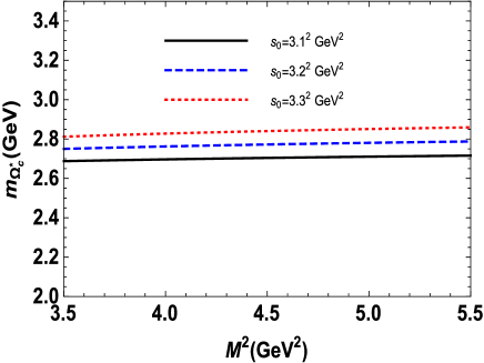
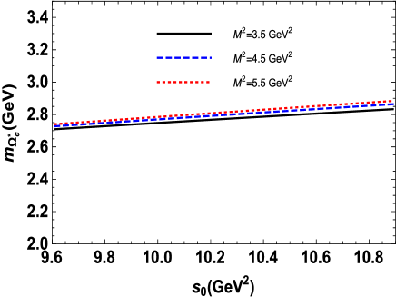
Figure 1: The mass of the ground-state $\Omega_{c}^{\star}$ baryon as a function of the Borel parameter $M^{2}$ at fixed $s_{0}$ (left panel), and as a function of the continuum threshold $s_{0}$ at fixed $M^{2}$ (right panel).

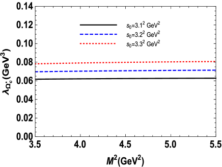
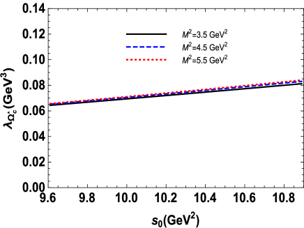
Figure 2: The dependence of the $\Omega_{c}^{\star}$ baryon’s residue $\lambda_{\Omega_{c}^{\star}}$ on the Borel parameter $M^{2}$ at chosen values of $s_{0}$ (left panel), and on the $s_{0}$ at fixed $M^{2}$ (right panel).

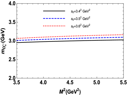
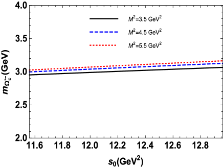
Figure 3: The same as in Fig. 1, but for the orbitally excited $\Omega_{c}^{\star-}$ baryon.

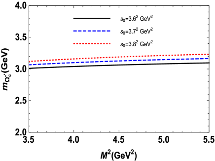
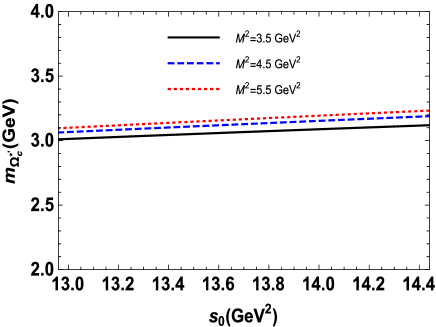
Figure 4: The same as in Fig. 1, but for the radially excited $\Omega_{c}^{\star\prime}$ baryon.

It is instructive to explore the ”convergence” of the iterative process used in the present work to evaluate parameters of the $\Omega_{c}$ baryons. It is known, that the ground-state contributes dominantly to the spectral density. The excited states included into the sum rules are sub-leading terms. To quantify this statement we calculate the pole contribution (PC) to the sum rules in the successive stages of the iterative process to reveal effects due to the ground-state and excited baryons. To this end, we fix the Borel parameter $M^{2}=4.5\ \mathrm{GeV}^{2}$ (for spin-1/2 baryons also $\cos\theta=-0.5$) and compute the PC at each stage using for the continuum threshold $s_{0}$ its upper limit from the relevant intervals (see, Tables 1 and 2). We start from the spin-1/2 baryons and from the ”ground-state + continuum” phase, and find that PC arising from $\Omega_{c}$ equals to $44\%$ of the result. Computations in the ”ground-state + 1P state + continuum” step allows us to fix the total PC from $\Omega_{c}$ and $\Omega_{c}^{-}$ baryons at the level $58\%$ of the whole prediction, or $14\%$ effect appearing due to $\Omega_{c}^{-}$. Finally, in the ”ground-state + 1P + 2S states + continuum” stage the PC arising from the $\Omega_{c}$, $\Omega_{c}^{-}$ and $\Omega_{c}^{\prime}$ baryons amounts to $68\%$ of the sum rules, which indicates $10\%$ contribution of the $\Omega_{c}^{\prime}$ baryon. The same analysis carried out for the spin-3/2 baryons leads to the following results: the ground-state baryon $\Omega_{c}^{\star}$ forms $41\%$ of the sum rule, whereas the excited states $\Omega_{c}^{\star-}$ and $\Omega_{c}^{\star\prime}$ constitute $15\%$ and $9\%$ of the whole prediction, respectively. It is worth noting that dependence of the presented estimations on $M^{2}$ and $\cos\theta$ is negligible.

It is seen, that the procedure adopted in the present work is consistent with general principles of the sum rule calculations. Because contributions of the higher excited states decrease, it is legitimate to restrict analysis by considering only two of them. But there are another reasons to truncate the iterative process at this phase. Indeed, the next spin-1/2 excited baryons in this range should be $(2P,1/2^{-})$ and $(3S,1/2^{+})$ states. By taking into account the mass splitting between $\Omega_{c}$ and first orbitally and radially excited $\Omega_{c}^{-}$ and $\Omega_{c}^{\prime}$ baryons, it is not difficult to anticipate that masses of the $(2P,1/2^{-})$ and $(3S,1/2^{+})$ states will be higher than recent LHCb data. The same arguments are valid for the spin-3/2 baryons, as well. The parameters of the higher excited states of $\Omega_{c}$ and $\Omega_{c}^{\star}$ baryons may provide a valuable information on their properties, which are interesting for hadron spectroscopy, nevertheless, this task is beyond the scope of the present investigation.

Basing on the results for the masses of $\Omega_{c}^{0}$ baryons, taking into account the central values in the sum rules’ predictions, and comparing them with LHCb data we, at this stage of our investigations, assign the orbitally and radially excited $\Omega_{c}^{0}$ baryons to be newly discovered states, as it is shown in Table 3. Thus, we have correlated the excited $\Omega_{c}^{0}$ baryons to states, which were recently observed by the LHCb Collaboration. Nevertheless, we consider this assignment as a preliminary one, because systematic errors in sum rule calculations are significant, and robust conclusions can be drawn only after analysis of the width of decays $\Omega_{c}^{0}\rightarrow\Xi_{c}^{+}K^{-}$ and $\Omega_{c}^{0}\rightarrow\Xi_{c}^{\prime+}K^{-}$.

	$\Omega_{c}^{0}$	$\Omega_{c}(2770)^{0}$	$\Omega_{c}(3000)^{0}$	$\Omega_{c}(3050)^{0}$	$\Omega_{c}(3066)^{0}$	$\Omega_{c}(3090)^{0}$	$\Omega_{c}(3119)^{0}$
	($\mathrm{M}eV$)	($\mathrm{M}eV$)	($\mathrm{M}eV$)	($\mathrm{M}eV$)	($\mathrm{M}eV$)	($\mathrm{M}eV$)	($\mathrm{M}eV$)
$(n,J^{P})$	$(1S,\frac{1}{2}^{+})$	$(1S,\frac{3}{2}^{+})$	$(1P,\frac{1}{2}^{-})$	$(1P,\frac{3}{2}^{-})$	$(2S,\frac{1}{2}^{+})$	$-$	$(2S,\frac{3}{2}^{+})$
Ref. LHCb	$-$	$-$	$3000.4\pm 0.2\pm 0.1$	$3050.2\pm 0.1\pm 0.1$	$3065.6\pm 0.1\pm 0.3$	$3090.2\pm 0.3\pm 0.5$	$3119.1\pm 0.3\pm 0.9$
Ref. Olive:2016xmw	$2695.2\pm 1.7$	$2765.9\pm 2.0$	$-$	$-$	$-$	$-$	$-$
This w.	$2685\pm 123$	$2769\pm 89$	$2990\pm 129$	$3056\pm 103$	$3075\pm 142$	$-$	$3119\pm 108$

Table 3: Our results for the masses of $\Omega_{c}^{0}$ baryons with spins $1/2$ and $3/2$, and experimental data from Refs. LHCb ; Olive:2016xmw .

III $\Omega_{c}^{-}$ and $\Omega_{c}^{\prime}$ transitions to $\Xi_{c}^{+}K^{-}$

The results for the masses of the excited $\Omega_{c}^{0}$ baryons show that all of them are above the $\Xi_{c}^{+}K^{-}$ threshold. Hence, these four states can decay through the $\Omega_{c}^{0}\to\Xi_{c}^{+}K^{-}$ channels.

In this section we study the vertices $\Omega_{c}^{-}\Xi_{c}^{+}K^{-}$ and $\Omega_{c}^{\prime}\Xi_{c}^{+}K^{-}$, and calculate corresponding strong couplings $g_{\Omega^{-}\Xi K}$ and $g_{\Omega^{\prime}\Xi K}$ (the sub-index $c$ is omitted from the baryons for simplicity), which are necessary to calculate widths of the decays $\Omega_{c}^{-}\rightarrow\Xi_{c}^{+}K^{-}$ and $\Omega_{c}^{\prime}\rightarrow\Xi_{c}^{+}K^{-}$. To this end we introduce the correlation function

$$\Pi(p,q)=i\int d^{4}xe^{ipx}\langle K(q)|\mathcal{T}\{\eta_{\Xi_{c}}(x)\overline{\eta}(0)\}|0\rangle,$$ (15)

where $\eta_{\Xi_{c}}(x)$ is the interpolating current for the $\Xi_{c}^{+}$ baryon. The $\Xi_{c}^{+}$ belongs to the anti-triplet configuration of the heavy baryons with a single heavy quark. Its current is anti-symmetric with respect to exchange of the two light quarks, and has the form

$$\eta_{\Xi_{c}} = \frac{1}{\sqrt{6}}\epsilon^{abc}\left\{2\left(u^{aT}Cs^{b}\right)\gamma_{5}c^{c}+2\beta\left(u^{aT}C\gamma_{5}s^{b}\right)c^{c}\right.$$ (16)

$$+\left(u^{aT}Cc^{b}\right)\gamma_{5}s^{c}+\beta\left(u^{aT}C\gamma_{5}c^{b}\right)s^{c}$$

$$\left.+\left(c^{aT}Cs^{b}\right)\gamma_{5}u^{c}+\beta\left(c^{aT}C\gamma_{5}s^{b}\right)u^{c}\right\}.$$

We first represent the correlation function $\Pi(p,q)$ using the parameters of the involved baryons, and, by this manner determine the phenomenological side of the sum rules. We get

$$\Pi^{\mathrm{Phys}}(p,q)=\frac{\langle 0|\eta_{\Xi_{c}}|\Xi_{c}(p,s)\rangle}{p^{2}-m_{\Xi_{c}}^{2}}\langle K(q)\Xi_{c}(p,s)|\Omega_{c}^{-}(p^{\prime},s^{\prime})\rangle$$

$$\times\frac{\langle\Omega_{c}^{-}(p^{\prime},s^{\prime})|\overline{\eta}|0\rangle}{p^{\prime 2}-\widetilde{m}^{2}}+\frac{\langle 0|\eta_{\Xi_{c}}|\Xi_{c}(p,s)\rangle}{p^{2}-m_{\Xi_{c}}^{2}}$$

$$\times\langle K(q)\Xi_{c}(p,s)|\Omega_{c}^{\prime}(p^{\prime},s^{\prime})\rangle\frac{\langle\Omega_{c}^{\prime}(p^{\prime},s^{\prime})|\overline{\eta}|0\rangle}{p^{\prime}{}^{2}-m^{\prime 2}}+\ldots,$$ (17)

where $p^{\prime}=p+q,\ p$ and $q$ are the momenta of the $\Omega_{c},\ \Xi_{c}$ baryons and $K$ meson, respectively. In the last expression $m_{\Xi_{c}}$ is the mass of the $\Xi_{c}^{+}$ baryon. The dots in Eq. (17) stand for contributions of the higher resonances and continuum states. Note that in principle the ground state $\Omega_{c}^{0}$ baryon can also be included into the correlation function. However its mass remain considerably below the threshold $\Xi_{c}^{+}K^{-}$ and its decay to the final state $\Xi_{c}^{+}K^{-}$ is not kinematically allowed.

We introduce the matrix element of the $\Xi_{c}^{+}$ baryon

$$\langle 0|\eta_{\Xi}|\Xi_{c}(p,s)\rangle=\lambda_{\Xi_{c}}u(p,s),$$

and define the strong couplings:

$$\langle K(q)\Xi_{c}(p,s)|\Omega_{c}^{\prime}(p^{\prime},s^{\prime})\rangle=g_{\Omega^{\prime}\Xi K}\overline{u}(p,s)\gamma_{5}u(p^{\prime},s^{\prime}),$$

$$\langle K(q)\Xi_{c}(p,s)|\Omega_{c}^{-}(p^{\prime},s^{\prime})\rangle=g_{\Omega^{-}\Xi K}\overline{u}(p,s)u(p^{\prime},s^{\prime}).$$

Then using the matrix elements of the $\Omega_{c}^{-}$ and $\Omega_{c}^{\prime}$ baryons, and performing the summation over $s$ and $s^{\prime}$ we recast the function $\Pi^{\mathrm{Phys}}(p,q)$ into the form:

$$\Pi^{\mathrm{Phys}}(p,q)=-\frac{g_{\Omega^{-}\Xi K}\lambda_{\Xi_{c}}\widetilde{\lambda}}{(p^{2}-m_{\Xi_{c}}^{2})(p^{\prime}{}^{2}-\widetilde{m}^{2})}(\not{p}+m_{\Xi_{c}})$$

$$\times\left(\not{p}+\not{q}+\widetilde{m}\right)\gamma_{5}+\frac{g_{\Omega^{\prime}\Xi K}\lambda_{\Xi_{c}}\lambda^{\prime}}{(p^{2}-m_{\Xi_{c}}^{2})(p^{\prime}{}^{2}-m^{\prime 2})}$$

$$\times(\not{p}+m_{\Xi_{c}})\gamma_{5}\left(\not{p}+\not{q}+m^{\prime}\right)+\ldots.$$ (19)

The double Borel transformation on the variables $p^{2}$ and $p^{\prime 2}$ applied to $\Pi^{\mathrm{Phys}}(p,q)$ yields

$$\mathcal{B}\Pi^{\mathrm{Phys}}(p,q)=g_{\Omega^{-}\Xi K}\lambda_{\Xi_{c}}\widetilde{\lambda}e^{-\widetilde{m}^{2}/M_{1}^{2}}e^{-m_{\Xi_{c}}^{2}/M_{2}^{2}}$$

$$\times\left\{\not{q}\not{p}\gamma_{5}-m_{\Xi_{c}}\not{q}\gamma_{5}-\left(\widetilde{m}+m_{\Xi_{c}}\right)\not{p}\gamma_{5}\right.$$

$$\left.+\left[m_{K}^{2}-\widetilde{m}(\widetilde{m}+m_{\Xi_{c}})\right]\gamma_{5}\right\}+g_{\Omega^{\prime}\Xi K}\lambda_{\Xi_{c}}\lambda^{\prime}$$

$$\times e^{-m^{\prime 2}/M_{1}^{2}}e^{-m_{\Xi_{c}}^{2}/M_{2}^{2}}\left\{\not{q}\not{p}\gamma_{5}-m_{\Xi_{c}}\not{q}\gamma_{5}+\left(m^{\prime}-m_{\Xi_{c}}\right)\not{p}\gamma_{5}\right.$$

$$\left.+\left[m_{K}^{2}-m^{\prime}(m^{\prime}-m_{\Xi_{c}})\right]\gamma_{5}\right\},$$ (20)

where $m_{K}^{2}=q^{2}$ is the mass of the $K$ meson, and $M_{1}^{2}$ and $M_{2}^{2}$ are the Borel parameters.

As is seen, there are different structures in Eq. (20), which can be used to derive the sum rules for the strong couplings. We work with the structures $\not{q}\not{p}\gamma_{5}$ and $\not{p}\gamma_{5}$. Separating the relevant terms in the Borel transformation of the correlation function $\Pi^{\mathrm{OPE}}(p,\,q)$ computed employing the quark-gluon degrees of freedom we get:

$$g_{\Omega^{-}\Xi K}=\frac{e^{\widetilde{m}^{2}/M_{1}^{2}}e^{m_{\Xi_{c}}^{2}/M_{2}^{2}}}{\lambda_{\Xi_{c}}\widetilde{\lambda}(m^{\prime}+\widetilde{m})}\left[(m^{\prime}-m_{\Xi_{c}})\mathcal{B}\Pi_{1}^{\mathrm{{}^{\prime}OPE}}-\mathcal{B}\Pi_{2}^{\mathrm{{}^{\prime}OPE}}\right],$$ (21)

and

$$g_{\Omega^{\prime}\Xi K}=\frac{e^{m^{\prime 2}/M_{1}^{2}}e^{m_{\Xi_{c}}^{2}/M_{2}^{2}}}{\lambda_{\Xi_{c}}\lambda^{\prime}(m^{\prime}+\widetilde{m})}\left[(\widetilde{m}+m_{\Xi_{c}})\mathcal{B}\Pi_{1}^{\mathrm{{}^{\prime}OPE}}+\mathcal{B}\Pi_{2}^{\mathrm{{}^{\prime}OPE}}\right],$$ (22)

where $\Pi_{1}^{\mathrm{{}^{\prime}OPE}}(p^{2},\,p^{\prime 2})$ and $\Pi_{2}^{\mathrm{{}^{\prime}OPE}}(p^{2},\,p^{\prime 2})$ are the invariant amplitudes corresponding to structures $\not{q}\not{p}\gamma_{5}$ and $\not{p}\gamma_{5}$, respectively.

The general expressions obtained above contain two Borel parameters $M_{1}^{2}$ and $M_{1}^{2}$. But in our analysis we choose

$$M_{1(2)}^{2}=2M^{2},\,\,M^{2}=\frac{M_{1}^{2}M_{2}^{2}}{M_{1}^{2}+M_{2}^{2}},$$ (23)

which is traditionally justified by a fact that masses of the involved heavy baryons $\Omega_{c}^{0}$ and $\Xi_{c}^{+}$ are close to each other.

Using the couplings $g_{\Omega^{-}\Xi K}$ and $g_{\Omega^{\prime}\Xi K}$ we can easily calculate the width of $\Omega_{c}^{-}\rightarrow\Xi_{c}^{+}K^{-}$ and $\Omega_{c}^{\prime}\rightarrow\Xi_{c}^{+}K^{-}$ decays. After some computations we obtain:

$$\Gamma\left(\Omega_{c}^{-}\rightarrow\Xi_{c}^{+}K^{-}\right) = \frac{g_{\Omega^{-}\Xi K}^{2}}{8\pi\widetilde{m}^{2}}\left[(\widetilde{m}+m_{\Xi_{c}})^{2}-m_{K}^{2}\right]$$ (24)

$$\times f(\widetilde{m},m_{\Xi_{c}},m_{K}).$$

and

$$\Gamma\left(\Omega_{c}^{\prime}\rightarrow\Xi_{c}^{+}K^{-}\right) = \frac{g_{\Omega^{\prime}\Xi K}^{2}}{8\pi m^{\prime 2}}\left[(m^{\prime}-m_{\Xi_{c}})^{2}-m_{K}^{2}\right]$$ (25)

$$\times f(m^{\prime},m_{\Xi_{c}},m_{K}),$$

In expressions above the function $f(x,y,z)$ is given as:

$$f(x,y,z)=\frac{1}{2x}\sqrt{x^{4}+y^{4}+z^{4}-2x^{2}y^{2}-2x^{2}z^{2}-2y^{2}z^{2}}.$$

The QCD side of the correlation function $\Pi^{\mathrm{OPE}}(p,q)$ can be found by contracting quark fields, and inserting into the obtained expression relevant propagators. The remaining non-local quark fields $\overline{s}_{\alpha}^{a}u_{\beta}^{b}$ have to be expanded using

$$\overline{s}_{\alpha}^{a}u_{\beta}^{b}=\frac{1}{4}\Gamma_{\beta\alpha}^{i}(\overline{s}^{a}\Gamma^{i}u^{b}),$$

where $\ \Gamma^{i}=1,\ \gamma_{5},\ \gamma_{\mu},\ i\gamma_{5}\gamma_{\mu},\ \sigma_{\mu\nu}/\sqrt{2}$ is the full set of Dirac matrices. Sandwiched between the K-meson and vacuum states these terms, as well as ones generated by insertion of the gluon field strength tensor $G_{\lambda\rho}(uv)$  from quark propagators, give rise to the K-meson’s distribution amplitudes of various quark-gluon contents and twists. Both in analytical and numerical calculations we take into account the K-meson DAs up to twist-4 and employ their explicit expressions from Ref. Ball:2006wn .

Apart from parameters in the distribution amplitudes, the sum rules for the couplings depend also on numerical values of the $\Xi_{c}^{+}$ baryon’s mass and pole residue. In numerical calculations we utilize

$$m_{\Xi_{c}}=2467.8^{+0.4}_{-0.6}\ \mathrm{MeV},\ \lambda_{\Xi_{c}}=0.054\pm 0.020\ \mathrm{GeV}^{3},$$ (26)

from Refs. Olive:2016xmw and Azizi:2016dmr , respectively. The Borel and threshold parameters for the decay of a baryon are chosen exactly as in computations of its mass. The auxiliary parameters $\beta$ in the interpolating currents of $\Omega_{c}^{0}$ and $\Xi_{c}^{+}$ baryons are taken equal to each other and varied within the limits $\cos\theta\in[-0.75,-0.3]$ and $[0.3,0.75]$, which are a little bit extended compared to the mass rules (see, Eq. (14)).

Numerical calculations lead to the following values for the strong couplings

$$g_{\Omega^{-}\Xi K}=0.48\pm 0.09,\ \ g_{\Omega^{\prime}\Xi K}=6.18\pm 1.92.$$ (27)

The predictions for the width of $\Omega_{c}^{-}\to\Xi_{c}^{+}K^{-}$ and $\Omega_{c}^{\prime}\to\Xi_{c}^{+}K^{-}$ decays are collected in Table 4 and compared with the LHCb data and results of other theoretical works.

$\Omega_{c}^{0}$	$\Omega_{c}(3000)^{0}$	$\Omega_{c}(3050)^{0}$	$\Omega_{c}(3066)^{0}$	$\Omega_{c}(3090)^{0}$	$\Omega_{c}(3119)^{0}$
	($\mathrm{MeV}$)	($\mathrm{MeV}$)	($\mathrm{M}eV$)	($\mathrm{MeV}$)	($\mathrm{MeV}$)
Ref. LHCb	$4.5\pm 0.6\pm 0.3$	$0.8\pm 0.2\pm 0.1$	$3.5\pm 0.4\pm 0.2$	$8.7\pm 1.0\pm 0.8$	$1.1\pm 0.8\pm 0.4$
This work	$4.7\pm 1.2$	$0.6\pm 0.2$	$6.4\pm 1.7$	$-$	$1.9\pm 0.6$
Ref. Wang:2017hej	$4.18$	$1.12$	$2.0$	$4.71$	$0.074$
Ref. Chen:2017	$-$	$2.7$	$3.3$	$8.8$	$0.7$

Table 4: The theoretical predictions and experimental data for width of the $\Omega_{c}^{0}$ states.

IV $\Omega_{c}^{\star-}\to\Xi_{c}^{+}K^{-}$, $\Omega_{c}^{\star\prime}\to\Xi_{c}^{+}K^{-}$ and $\Omega_{c}^{\star\prime}\to\Xi_{c}^{\prime+}K^{-}$ decays

The decays of the spin-$3/2$ baryons $\Omega_{c}^{\star\prime}$ and $\Omega_{c}^{\star-}$ to $\Xi_{c}^{+}\,K^{-}$ can analyzed as it has been done for the spin-$1/2$ baryons. Additionally, we take into account, that the radially excited $\Omega_{c}^{\star\prime}$ baryon can decay through the channel $\Omega_{c}^{\star\prime}\rightarrow\Xi_{c}^{\prime+}\,K^{-}$, as well. The $\Xi_{c}^{\prime+}$ is spin-$1/2$ ground-state baryon, and it belongs to sextet part of the heavy baryons. Its interpolating current should be symmetric under exchange of the two light quarks. In this section we consider these three decay processes.

Again we start from the same correlation function, but with the current $\eta(x)$ replaced by $\eta_{\mu}(x)$:

$$\Pi_{\mu}(p,q)=i\int d^{4}xe^{ipx}\langle K(q)|\mathcal{T}\{\eta_{\Xi_{c}}(x)\overline{\eta}_{\mu}(0)\}|0\rangle.$$ (28)

We define the strong couplings $g_{\Omega^{\star-}\Xi K}$ and $g_{\Omega^{\star\prime}\Xi K}$ through matrix elements

$$\langle K(q)\Xi_{c}(p,s)|\Omega_{c}^{\ast-}(p^{\prime},s^{\prime})\rangle=g_{\Omega^{\star-}\Xi K}\overline{u}(p,s)\gamma_{5}u_{\alpha}(p^{\prime},s^{\prime})q^{\alpha},$$

$$\langle K(q)\Xi_{c}(p,s)|\Omega_{c}^{\ast\prime}(p^{\prime},s^{\prime})\rangle=g_{\Omega^{\star\prime}\Xi K}\overline{u}(p,s)u_{\alpha}(p^{\prime},s^{\prime})q^{\alpha}.$$

and for $\Pi_{\mu}^{\mathrm{Phys}}(p,q)$ obtain the following expression:

$$\Pi_{\mu}^{\mathrm{Phys}}(p,q)=\frac{g_{\Omega^{\star-}\Xi K}\lambda_{\Xi_{c}}\widetilde{\lambda}}{(p^{2}-m_{\Xi_{c}}^{2})(p^{\prime}{}^{2}-\widetilde{m}^{2})}q^{\alpha}(\not{p}+m_{\Xi_{c}})\gamma_{5}$$

$$\times\left(\not{p}+\not{q}+\widetilde{m}\right)F_{\alpha\mu}(\widetilde{m})\gamma_{5}-\frac{g_{\Omega^{\star\prime}\Xi K}\lambda_{\Xi_{c}}\lambda^{\prime}}{(p^{2}-m_{\Xi_{c}}^{2})(p^{\prime 2}-m^{\prime 2})}$$

$$\times q^{\alpha}(\not{p}+m_{\Xi_{c}})\left(\not{p}+\not{q}+m^{\prime}\right)F_{\alpha\mu}(m^{\prime})+\ldots,$$ (30)

where we have used the shorthand notation

$$F_{\alpha\mu}(m)=g_{\alpha\mu}-\frac{1}{3}\gamma_{\alpha}\gamma_{\mu}-\frac{2}{3m^{2}}(p_{\alpha}+q_{\alpha})(p_{\mu}+q_{\mu})$$

$$+\frac{1}{3m}\left[(p_{\alpha}+q_{\alpha})\gamma_{\mu}-(p_{\mu}+q_{\mu})\gamma_{\alpha}\right].$$ (31)

For the Borel transformation of $\Pi_{\mu}^{\mathrm{Phys}}(p,q)$ we get

$$\mathcal{B}\Pi_{\mu}^{\mathrm{Phys}}(p,q)=g_{\Omega^{\star-}\Xi K}\lambda_{\Xi_{c}}\widetilde{\lambda}e^{-\widetilde{m}^{2}/M_{1}^{2}}e^{-m_{\Xi_{c}}^{2}/M_{2}^{2}}q^{\alpha}$$

$$\times(\not{p}+m_{\Xi_{c}})\gamma_{5}\left(\not{p}+\not{q}+\widetilde{m}\right)F_{\alpha\mu}(\widetilde{m})\gamma_{5}-g_{\Omega^{\star\prime}\Xi K}\lambda_{\Xi_{c}}\lambda^{\prime}$$

$$\times e^{-m^{\prime 2}/M_{1}^{2}}e^{-m_{\Xi_{c}}^{2}/M_{2}^{2}}q^{\alpha}(\not{p}+m_{\Xi_{c}})\left(\not{p}+\not{q}+m^{\prime}\right)F_{\alpha\mu}(m^{\prime}).$$

To extract the sum rules we choose the structures $\not{q}\not{p}\gamma_{\mu}$ and $\not{q}q_{\mu}$.  The same structures should be isolated in $\mathcal{B}\Pi_{\mu}^{\mathrm{QCD}}(p,q)$ and matched with ones from $\mathcal{B}\Pi_{\mu}^{\mathrm{Phys}}(p,q)$. The final formulas for the strong couplings are rather lengthy, therefore we refrain from providing their explicit expressions.

The knowledge of the strong couplings allows us to find the widths of the corresponding decay channels. Thus, the width of the $\Omega_{c}^{\ast-}\rightarrow\Xi_{c}^{+}K^{-}$ decay can be obtained as

$$\Gamma(\Omega_{c}^{\ast-} \rightarrow \Xi_{c}^{+}K^{-})=\frac{g_{\Omega^{\star-}\Xi K}^{2}}{24\pi\widetilde{m}^{2}}\left[(\widetilde{m}-m_{\Xi_{c}})^{2}-m_{K}^{2}\right]$$ (33)

$$\times f^{3}(\widetilde{m},m_{\Xi_{c}},m_{K}).$$

whereas for $\Gamma(\Omega_{c}^{\ast\prime}\rightarrow\Xi_{c}^{+}K^{-})$ we get

$$\Gamma(\Omega_{c}^{\ast\prime} \rightarrow \Xi_{c}^{+}K^{-})=\frac{g_{\Omega^{\star\prime}\Xi K}^{2}}{24\pi m^{\prime 2}}\left[(m^{\prime}+m_{\Xi_{c}})^{2}-m_{K}^{2}\right]$$ (34)

$$\times f^{3}(m^{\prime},m_{\Xi_{c}},m_{K}),$$

In order to find $g_{\Omega^{\star\prime}\Xi^{\prime}K}$ corresponding to the vertex $\Omega_{c}^{\star\prime}\Xi_{c}^{\prime+}K^{-}$, we again use the correlation function $\Pi_{\mu}(p,q)$, but with the current $\eta_{\Xi_{c}^{\prime}}$,

$$\eta_{\Xi_{c}^{\prime}}=-\frac{1}{\sqrt{2}}\epsilon^{abc}\left\{\left(u^{aT}Cc^{b}\right)\gamma_{5}s^{c}+\beta\left(u^{aT}C\gamma_{5}c^{b}\right)s^{c}\right.$$

$$\left.-\left[\left(c^{aT}Cs^{b}\right)\gamma_{5}u^{c}+\beta\left(c^{aT}C\gamma_{5}s^{b}\right)u^{c}\right]\right\}.$$ (35)

We skip details and provide below only final expression for the double Borel transformation of the term $\sim\not{q}\not{p}\gamma_{\mu}$ in $\widetilde{\Pi}_{\mu}^{\mathrm{Phys}}(p,q)$, which is utilized to derive the required sum rule

$$\mathcal{B}\widetilde{\Pi}_{\mu}^{\mathrm{Phys}}(p,q)=-\frac{g_{\Omega^{\star\prime}\Xi^{\prime}K}\lambda_{\Xi_{c}^{\prime}}\lambda^{\prime}}{6m^{\prime}}e^{-m^{\prime 2}/M_{1}^{2}}e^{-m_{\Xi_{c}^{\prime}}^{2}/M_{2}^{2}}$$

$$\times\left[\left(m^{\prime}+m_{\Xi_{c}^{\prime}}\right)^{2}-m_{K}^{2}\right]\not{q}\not{p}\gamma_{\mu}.$$ (36)

In Eq. (36) $m_{\Xi_{c}^{\prime}}$ and $\lambda_{\Xi_{c}^{\prime}}$ are the $\Xi_{c}^{\prime+}$ baryon’s mass and pole residue, respectively.

The coupling $g_{\Omega^{\star\prime}\Xi^{\prime}K}$ and widths of the decay $\Omega_{c}^{\ast\prime}\rightarrow\Xi_{c}^{\prime+}K^{-}$ are given be the expressions:

$$g_{\Omega^{\prime}\Xi^{\prime}K}=-\frac{e^{m^{\prime 2}/M_{1}^{2}}e^{m_{\Xi_{c}^{\prime}}^{2}/M_{2}^{2}}6m^{\prime}}{\lambda_{\Xi_{c}^{\prime}}\lambda^{\prime}\left[(m^{\prime}+m_{\Xi_{c}^{\prime}})^{2}-m_{K}^{2}\right]}\mathcal{B}\widetilde{\Pi}^{\mathrm{OPE}},$$

and

$$\Gamma(\Omega_{c}^{\star\prime} \rightarrow \Xi_{c}^{\prime+}K^{-})=\frac{g_{\Omega^{\star\prime}\Xi^{\prime}K}^{2}}{24\pi m^{\prime 2}}\left[(m^{\prime}+m_{\Xi_{c}^{\prime}})^{2}-m_{K}^{2}\right]$$ (37)

$$\times f^{3}(m^{\prime},m_{\Xi_{c}^{\prime}},m_{K}).$$

In numerical computations for the mass and residue of the $\Xi_{c}^{\prime+}$ baryon we use

$$m_{\Xi_{c}^{\prime}}=2575.6\pm 3.1\ \mathrm{MeV},\ \lambda_{\Xi_{c}^{\prime}}=0.055\pm 0.016\ \mathrm{GeV}^{3},$$ (38)

which are borrowed from Refs. Olive:2016xmw and Wang:2009cr , respectively.

Numerical computations for the strong couplings yield (in $\mathrm{GeV}^{-1}$):

$$g_{\Omega^{\star-}\Xi K}=12.59\pm 1.78,\ \ g_{\Omega^{\star\prime}\Xi K}=0.75\pm 0.20,\$$

$$g_{\Omega^{\star\prime}\Xi^{\prime}K}=1.21\pm 0.41.$$ (39)

For the decay widths we get:

$$\Gamma(\Omega_{c}^{\star-}\rightarrow\Xi_{c}^{+}K^{-})=0.6\pm 0.2\,\ \mathrm{MeV},$$

$$\Gamma(\Omega_{c}^{\star\prime}\rightarrow\Xi_{c}^{+}K^{-})=1.3\pm 0.4\,\ \mathrm{MeV},$$

$$\Gamma(\Omega_{c}^{\star\prime}\rightarrow\Xi_{c}^{\prime+}K^{-})=0.6\pm 0.2\,\ \mathrm{MeV}.$$ (40)

Obtained predictions for widths of the $\Omega_{c}^{\star-}$ and $\Omega_{c}^{\star\prime}$ baryons are shown in Table 4: for $\Omega_{c}^{\star\prime}$ we present there a sum of its two possible decay channels.

V Discussion and Concluding remarks

In the present work we have investigated the newly discovered $\Omega_{c}^{0}$ baryons by means of QCD sum rule method. We have calculated masses and pole residues of the ground-state and first orbitally and radially excited $\Omega_{c}^{0}$ baryons with the spin-$1/2$ and -$3/2$. To this end, we have employed two-point QCD sum rule method and started from the ground-state baryons. We have derived required sum rules for $m_{\Omega_{c}}$ and $\lambda_{\Omega_{c}}$ using two different structures in the relevant correlation functions. The masses and residues of the ground-states have been treated as input information in the sum rules obtained to evaluate parameters of the first orbitally excited baryons. The same manipulations have been repeated also in the case of the radially excited states.

The predictions for the masses and residues obtained in the present work almost coincide with results of our previous paper Agaev:2017jyt excluding numerically small modifications in parameters of the radially excited baryons. This may be expected, because in the present work we have employed more sophisticated iterative scheme. Nevertheless, assignments for $\Omega_{c}^{0}$ made in Ref. Agaev:2017jyt remain valid here, as well (see, Table 3).

The widths of the $\Omega_{c}^{0}\to\Xi_{c}^{+}K^{-}$ decays, calculated in the context of the QCD full LCSR method, have allowed us to confirm an essential part of our previous conclusions. Thus, the mass and width of the $(1P,\,1/2^{-})$ and $(2S,\,3/2^{+})$ states are in a nice agreements with the same parameters of the $\Omega_{c}(3000)$ and $\Omega_{c}(3119)$ baryons, respectively. The mass of the orbitally excited state $(1P,\,3/2^{-})$ is close to $\Omega_{c}(3050)$. But it may be considered also as the $\Omega_{c}(3066)$ baryon. A decisive argument in favor of $\Omega_{c}(3050)$ is the width of the state $(1P,\,3/2^{-})$, which is in excellent agreement with LHCb measurements. As a result, we do not hesitate to confirm our previous assignment of $\Omega_{c}(3050)$ to be the baryon with $J^{P}=3/2^{-}$. Situation with the orbitally excited state $(2S,\,1/2^{+})$ is not quite clear. In fact, its mass and width, allow one to interpret it either as $\Omega_{c}(3066)$ or $\Omega_{c}(3090)$. We have kept in Tables 3 and 4 our previous classification of the $(2S,\,1/2^{+})$ state as the $\Omega_{c}(3066)$ baryon, but its interpretation as $\Omega_{c}(3090)$ is also legitimate.

The masses of the excited $\Omega_{c}^{0}$ baryons were predicted in theoretical literature long before the recent LHCb data. Most of them were made in the framework of different quark models (see, for example Refs. Ebert:2011kk ; Valcarce:2008dr ; Vijande:2012mk ; Shah:2016nxi ). Within the two-point QCD sum rule method problems of the $\Omega_{c}^{0}$ baryons were addressed in Refs. Wang:2007sqa ; Wang:2008hz ; Wang:2009cr ; Azizi:2015ksa , where the masses of the ground-state and excited $\Omega_{c}^{0}$ were found. Obtained in Refs. Azizi:2015ksa mass of $\Omega_{c}^{0}$ baryon with $J^{P}=3/2^{-}$

$$m_{\Omega_{c}^{\star}}=3080\pm 120\ \mathrm{GeV}$$ (41)

within errors agrees both with LHCb data and our present result for $(1P,\ 3/2^{-})$ state.

After discovery of the LHCb Collaboration, parameters of new states in the context of QCD sum rule approach have been also investigated in Refs. Wang:2017hej ; Aliev:2017led . In Ref. Wang:2017hej all of five states have been considered as negative-parity baryons, whereas in Ref. Aliev:2017led only two of them have been classified as negative-parity states. But lack of information about widths of $\Omega_{c}^{0}$ makes incomplete comparison of their results with available LHCb data.

A situation around excited $\Omega_{c}^{0}$ states remains controversial and unclear. Additional efforts of experimental collaborations are necessary to explore $\Omega_{c}^{0}$ states, mainly to fix their spin-parities.

Appendix A The correlation functions and quark propagators

The correlation function for the spin $1/2$ baryons

$$\Pi(p)=i\int d^{4}xe^{ipx}\langle 0|\mathcal{T}\{\eta(x)\overline{\eta}(0)\}|0\rangle,$$

in terms of the quark propagators takes the following form:

$$\Pi^{\mathrm{OPE}}(p)=\int d^{4}xe^{ipx}\frac{\epsilon\epsilon^{\prime}}{4}\left\{-\gamma_{5}S_{s}^{ca^{\prime}}(x)\widetilde{S}_{c}^{ab^{\prime}}(x)S_{s}^{bc^{\prime}}(x)\gamma_{5}+\gamma_{5}S_{s}^{ca^{\prime}}(x)\widetilde{S}_{c}^{bb^{\prime}}(x)S_{s}^{ac^{\prime}}(x)\gamma_{5}+\gamma_{5}S_{s}^{cb^{\prime}}(x)\widetilde{S}_{c}^{aa^{\prime}}(x)S_{s}^{bc^{\prime}}(x)\gamma_{5}\right.$$

$$-\gamma_{5}S_{s}^{cb^{\prime}}(x)\widetilde{S}_{c}^{ba^{\prime}}(x)S_{s}^{ac^{\prime}}(x)\gamma_{5}+\gamma_{5}S_{s}^{cc^{\prime}}(x)\gamma_{5}\left[-\mathrm{Tr}\left[S_{c}^{aa^{\prime}}(x)\widetilde{S}_{s}^{bb^{\prime}}(x)\right]+\mathrm{Tr}\left[S_{c}^{ab^{\prime}}(x)\widetilde{S}_{s}^{ba^{\prime}}(x)\right]-\mathrm{Tr}\left[S_{s}^{aa^{\prime}}(x)\widetilde{S}_{c}^{bb^{\prime}}(x)\right]\right.$$

$$\left.+\mathrm{Tr}\left[S_{s}^{ab^{\prime}}(x)\widetilde{S}_{c}^{ba^{\prime}}(x)\right]\right]+\beta\left[-\gamma_{5}S_{s}^{ca^{\prime}}(x)\gamma_{5}\widetilde{S}_{c}^{ab^{\prime}}(x)S_{s}^{bc^{\prime}}(x)+\gamma_{5}S_{s}^{ca^{\prime}}(x)\gamma_{5}\widetilde{S}_{c}^{bb^{\prime}}(x)S_{s}^{ac^{\prime}}(x)+\gamma_{5}S_{s}^{cb^{\prime}}(x)\gamma_{5}\widetilde{S}_{c}^{aa^{\prime}}(x)S_{s}^{bc^{\prime}}(x)\right.$$

$$\left.-\gamma_{5}S_{s}^{cb^{\prime}}(x)\gamma_{5}\widetilde{S}_{c}^{ba^{\prime}}(x)S_{s}^{ac^{\prime}}(x)-S_{s}^{ca^{\prime}}(x)\widetilde{S}_{c}^{ab^{\prime}}(x)\gamma_{5}S_{s}^{bc^{\prime}}(x)\gamma_{5}+S_{s}^{ca^{\prime}}(x)\widetilde{S}_{c}^{bb^{\prime}}(x)\gamma_{5}S_{s}^{ac^{\prime}}(x)\gamma_{5}+S_{s}^{cb^{\prime}}(x)\widetilde{S}_{c}^{aa^{\prime}}(x)\gamma_{5}S_{s}^{bc^{\prime}}(x)\gamma_{5}\right.$$

$$\left.-S_{s}^{cb^{\prime}}(x)\widetilde{S}_{c}^{ba^{\prime}}(x)\gamma_{5}S_{s}^{ac^{\prime}}(x)\gamma_{5}+\gamma_{5}S_{s}^{cc^{\prime}}(x)\left[-\mathrm{Tr}\left[S_{c}^{aa^{\prime}}(x)\gamma_{5}\widetilde{S}_{s}^{bb^{\prime}}(x)\right]+\mathrm{Tr}\left[S_{c}^{ab^{\prime}}(x)\gamma_{5}\widetilde{S}_{s}^{ba^{\prime}}(x)\right]-\mathrm{Tr}\left[S_{s}^{aa^{\prime}}(x)\gamma_{5}\widetilde{S}_{c}^{bb^{\prime}}(x)\right]\right.\right.$$

$$\left.+\mathrm{Tr}\left[S_{s}^{ab^{\prime}}(x)\gamma_{5}\widetilde{S}_{c}^{ba^{\prime}}(x)\right]\right]+S_{s}^{cc^{\prime}}(x)\gamma_{5}\left[-\mathrm{Tr}\left[S_{c}^{aa^{\prime}}(x)\widetilde{S}_{s}^{bb^{\prime}}(x)\gamma_{5}\right]+\mathrm{Tr}\left[S_{c}^{ab^{\prime}}(x)\widetilde{S}_{s}^{ba^{\prime}}(x)\gamma_{5}\right]-\mathrm{Tr}\left[S_{s}^{aa^{\prime}}(x)\widetilde{S}_{c}^{bb^{\prime}}(x)\gamma_{5}\right]\right.$$

$$\left.\left.+\mathrm{Tr}\left[S_{s}^{ab^{\prime}}(x)\widetilde{S}_{c}^{ba^{\prime}}(x)\gamma_{5}\right]\right]\right]+\beta^{2}\left[-S_{s}^{ca^{\prime}}(x)\gamma_{5}\widetilde{S}_{c}^{ab^{\prime}}(x)\gamma_{5}S_{s}^{bc^{\prime}}(x)+S_{s}^{ca^{\prime}}(x)\gamma_{5}\widetilde{S}_{c}^{bb^{\prime}}(x)\gamma_{5}S_{s}^{ac^{\prime}}(x)\right.$$

$$+S_{s}^{cb^{\prime}}(x)\gamma_{5}\widetilde{S}_{c}^{aa^{\prime}}(x)\gamma_{5}S_{s}^{bc^{\prime}}(x)-S_{s}^{cb^{\prime}}(x)\gamma_{5}\widetilde{S}_{c}^{ba^{\prime}}(x)\gamma_{5}S_{s}^{ac^{\prime}}(x)+S_{s}^{cc^{\prime}}(x)\left[\mathrm{Tr}\left[S_{c}^{ba^{\prime}}(x)\gamma_{5}\widetilde{S}_{s}^{ab^{\prime}}(x)\gamma_{5}\right]\right.$$

$$\left.\left.-\mathrm{Tr}\left[S_{c}^{bb^{\prime}}(x)\gamma_{5}\widetilde{S}_{s}^{aa^{\prime}}(x)\gamma_{5}\right]+\mathrm{Tr}\left[S_{s}^{ba^{\prime}}(x)\gamma_{5}\widetilde{S}_{c}^{ab^{\prime}}(x)\gamma_{5}\right]-\mathrm{Tr}\left[S_{c}^{bb^{\prime}}(x)\gamma_{5}\widetilde{S}_{c}^{aa^{\prime}}(x)\gamma_{5}\right]\right]\right\}.$$ (A.42)

For the correlation function of spin $3/2$ baryons we get:

$$\Pi_{\mu\nu}^{\mathrm{OPE}}(p)=\int d^{4}xe^{ipx}\frac{\epsilon\epsilon^{\prime}}{3}\left\{S_{c}^{ca^{\prime}}(x)\gamma_{\nu}\widetilde{S}_{s}^{ab^{\prime}}(x)\gamma_{\mu}S_{s}^{bc^{\prime}}(x)-S_{c}^{ca^{\prime}}(x)\gamma_{\nu}\widetilde{S}_{s}^{bb^{\prime}}(x)\gamma_{\mu}S_{s}^{ac^{\prime}}(x)-S_{c}^{cb^{\prime}}(x)\gamma_{\nu}\widetilde{S}_{s}^{aa^{\prime}}(x)\gamma_{\mu}S_{s}^{bc^{\prime}}(x)\right.$$

$$+S_{c}^{cb^{\prime}}(x)\gamma_{\nu}\widetilde{S}_{s}^{ba^{\prime}}(x)\gamma_{\mu}S_{s}^{ac^{\prime}}(x)+S_{s}^{ca^{\prime}}(x)\gamma_{\nu}\widetilde{S}_{c}^{ab^{\prime}}(x)\gamma_{\mu}S_{s}^{bc^{\prime}}(x)-S_{s}^{ca^{\prime}}(x)\gamma_{\nu}\widetilde{S}_{c}^{bb^{\prime}}(x)\gamma_{\mu}S_{s}^{ac^{\prime}}(x)+S_{s}^{ca^{\prime}}(x)\gamma_{\nu}\widetilde{S}_{s}^{ab^{\prime}}(x)\gamma_{\mu}S_{c}^{bc^{\prime}}(x)$$

$$-S_{s}^{ca^{\prime}}(x)\gamma_{\nu}\widetilde{S}_{s}^{bb^{\prime}}(x)\gamma_{\mu}S_{c}^{ac^{\prime}}(x)-S_{s}^{cb^{\prime}}(x)\gamma_{\nu}\widetilde{S}_{c}^{aa^{\prime}}(x)\gamma_{\mu}S_{s}^{bc^{\prime}}(x)+S_{s}^{cb^{\prime}}(x)\gamma_{\nu}\widetilde{S}_{c}^{ba^{\prime}}(x)\gamma_{\mu}S_{s}^{ac^{\prime}}(x)-S_{s}^{cb^{\prime}}(x)\gamma_{\nu}\widetilde{S}_{s}^{aa^{\prime}}(x)\gamma_{\mu}S_{c}^{bc^{\prime}}(x)$$

$$+S_{s}^{cb^{\prime}}(x)\gamma_{\nu}\widetilde{S}_{s}^{ba^{\prime}}(x)\gamma_{\mu}S_{c}^{ac^{\prime}}(x)-S_{s}^{cc^{\prime}}(x)\left[\mathrm{Tr}\left[S_{c}^{ba^{\prime}}(x)\gamma_{\nu}\widetilde{S}_{s}^{ab^{\prime}}(x)\gamma_{\mu}\right]-\mathrm{Tr}\left[S_{c}^{bb^{\prime}}(x)\gamma_{\nu}\widetilde{S}_{s}^{aa^{\prime}}(x)\gamma_{\mu}\right]+\mathrm{Tr}\left[S_{s}^{ba^{\prime}}(x)\gamma_{\nu}\widetilde{S}_{c}^{ab^{\prime}}(x)\gamma_{\mu}\right]\right.$$

$$\left.\left.-\mathrm{Tr}\left[S_{s}^{bb^{\prime}}(x)\gamma_{\nu}\widetilde{S}_{c}^{aa^{\prime}}(x)\gamma_{\mu}\right]\right]-S_{c}^{cc^{\prime}}(x)\left[\mathrm{Tr}\left[S_{s}^{ba^{\prime}}(x)\gamma_{\nu}\widetilde{S}_{s}^{ab^{\prime}}(x)\gamma_{\mu}\right]-\mathrm{Tr}\left[S_{s}^{bb^{\prime}}(x)\gamma_{\nu}\widetilde{S}_{s}^{aa^{\prime}}(x)\gamma_{\mu}\right]\right]\right\}.$$ (A.43)

In Eqs. (A.42) and (A.43) $\epsilon\epsilon^{\prime}=\epsilon^{abc}\epsilon^{a^{\prime}b^{\prime}c^{\prime}}$ and $\widetilde{S}_{s(c)}(x)=CS_{s(c)}^{T}(x)C$.

The quark propagators are important ingredients of sum rules calculations. Below we provide explicit expressions of the light and heavy quark propagators in the $x$-representation. For the light $q=u,d,s$ quarks we have

$$S_{q}^{ab}(x)=\frac{i\not{x}}{2\pi^{2}x^{4}}\delta_{ab}-\frac{m_{q}}{4\pi^{2}x^{2}}\delta_{ab}-\frac{\langle\overline{q}q\rangle}{12}\left(1-i\frac{m_{q}}{4}\not{x}\right)\delta_{ab}-\frac{x^{2}}{192}m_{0}^{2}\langle\overline{q}q\rangle\left(1-i\frac{m_{q}}{6}\not{x}\right)\delta_{ab}$$

$$-ig_{s}\int_{0}^{1}du\left\{\frac{\not{x}}{16\pi^{2}x^{2}}G_{ab}^{\mu\nu}(ux)\sigma_{\mu\nu}-\frac{iux_{\mu}}{4\pi^{2}x^{2}}G_{ab}^{\mu\nu}(ux)\gamma_{\nu}-\frac{im_{q}}{32\pi^{2}}G_{ab}^{\mu\nu}(ux)\sigma_{\mu\nu}\left[\ln\left(\frac{-x^{2}\Lambda^{2}}{4}\right)+2\gamma_{E}\right]\right\},$$ (A.44)

where $\gamma_{E}\simeq 0.577$ is the Euler constant and $\Lambda$ is the QCD scale parameter. We have also used the notation $G_{ab}^{\mu\nu}\equiv G_{A}^{\mu\nu}t_{ab}^{A},\ A=1,2,\ldots 8$, and $t^{A}=\lambda^{A}/2$, with $\lambda^{A}$ being the Gell-Mann matrices.

The heavy $Q=c,b$ quark propagators we get

$$S_{Q}^{ab}(x)=\frac{m_{Q}^{2}}{4\pi^{2}}\frac{K_{1}\left(m_{Q}\sqrt{-x^{2}}\right)}{\sqrt{-x^{2}}}\delta_{ab}+i\frac{m_{Q}^{2}}{4\pi^{2}}\frac{\not{x}K_{2}\left(m_{Q}\sqrt{-x^{2}}\right)}{\left(\sqrt{-x^{2}}\right)^{2}}\delta_{ab}-\frac{g_{s}m_{Q}}{16\pi^{2}}\int_{0}^{1}duG_{ab}^{\mu\nu}(ux)\left[(\sigma_{\mu\nu}\not{x}+\not{x}\sigma_{\mu\nu})\right.$$

$$\left.\times\frac{K_{1}\left(m_{Q}\sqrt{-x^{2}}\right)}{\sqrt{-x^{2}}}+2\sigma_{\mu\nu}K_{0}\left(m_{Q}\sqrt{-x^{2}}\right)\right].$$ (A.45)

The first two terms above is the free heavy quark propagator in the coordinate representation, and $K_{n}(z)$ are the modified Bessel functions of the second kind.

References

• (1) R. Aaij et al. [LHCb Collaboration], arXiv:1703.04639 [hep-ex].
• (2) C. Patrignani et al. [Particle Data Group], Chin. Phys. C 40, 100001 (2016).
• (3) S. Capstick and N. Isgur, Phys. Rev. D 34, 2809 (1986).
• (4) E. Bagan, M. Chabab, H. G. Dosch and S. Narison, Phys. Lett. B 278, 367 (1992).
• (5) E. Bagan, M. Chabab, H. G. Dosch and S. Narison, Phys. Lett. B 287, 176 (1992).
• (6) G. Chiladze and A. F. Falk, Phys. Rev. D 56, R6738 (1997).
• (7) C. S. Huang, A. l. Zhang and S. L. Zhu, Phys. Lett. B 492, 288 (2000).
• (8) D. W. Wang, M. Q. Huang and C. Z. Li, Phys. Rev. D 65, 094036 (2002).
• (9) D. Ebert, R. N. Faustov and V. O. Galkin, Phys. Lett. B 659, 612 (2008).
• (10) D. Ebert, R. N. Faustov and V. O. Galkin, Phys. Rev. D 84, 014025 (2011).
• (11) H. Garcilazo, J. Vijande and A. Valcarce, J. Phys. G 34, 961 (2007).
• (12) A. Valcarce, H. Garcilazo and J. Vijande, Eur. Phys. J. A 37, 217 (2008).
• (13) W. Roberts and M. Pervin, Int. J. Mod. Phys. A 23, 2817 (2008).
• (14) Z. G. Wang, Eur. Phys. J. C 54, 231 (2008).
• (15) Z. G. Wang, Eur. Phys. J. C 61, 321 (2009).
• (16) Z. G. Wang, Phys. Lett. B 685, 59 (2010).
• (17) J. Vijande, A. Valcarce, T. F. Carames and H. Garcilazo, Int. J. Mod. Phys. E 22, 1330011 (2013).
• (18) T. Yoshida, E. Hiyama, A. Hosaka, M. Oka and K. Sadato, Phys. Rev. D 92, 114029 (2015).
• (19) R. G. Edwards et al. [Hadron Spectrum Collaboration], Phys. Rev. D 87, 054506 (2013).
• (20) M. Padmanath, R. G. Edwards, N. Mathur and M. Peardon, arXiv:1311.4806 [hep-lat].
• (21) H. X. Chen, W. Chen, Q. Mao, A. Hosaka, X. Liu and S. L. Zhu, Phys. Rev. D 91, 054034 (2015).
• (22) H. X. Chen, Q. Mao, A. Hosaka, X. Liu and S. L. Zhu, Phys. Rev. D 94, 114016 (2016).
• (23) Z. Shah, K. Thakkar, A. K. Rai and P. C. Vinodkumar, Chin. Phys. C 40, 123102 (2016).
• (24) T. M. Aliev, K. Azizi, T. Barakat and M. Savci, Phys. Rev. D 92, 036004 (2015).
• (25) K. Azizi and H. Sundu, Eur. Phys. J. Plus 132, 22 (2017).
• (26) S. L. Zhu, W. Y. P. Hwang and Z. S. Yang, Phys. Rev. D 56, 7273 (1997).
• (27) T. M. Aliev, K. Azizi and A. Ozpineci, Nucl. Phys. B 808, 137 (2009).
• (28) T. M. Aliev, K. Azizi and A. Ozpineci, Phys. Rev. D 79, 056005 (2009).
• (29) T. M. Aliev, K. Azizi and M. Savci, Nucl. Phys. A 852, 141 (2011).
• (30) T. M. Aliev, K. Azizi and M. Savci, Eur. Phys. J. C 71, 1675 (2011).
• (31) T. M. Aliev, K. Azizi, M. Savci and V. S. Zamiralov, Phys. Rev. D 83, 096007 (2011).
• (32) T. M. Aliev, K. Azizi and M. Savci, Nucl. Phys. A 870-871, 58 (2011).
• (33) T. M. Aliev, K. Azizi and M. Savci, Eur. Phys. J. A 47, 125 (2011).
• (34) T. M. Aliev, K. Azizi and M. Savci, Phys. Lett. B 690, 164 (2010).
• (35) S. S. Agaev, K. Azizi and H. Sundu, arXiv:1703.07091 [hep-ph].
• (36) H. X. Chen, Q. Mao, W. Chen, A. Hosaka, X. Liu and S. L. Zhu, arXiv:1703.07703 [hep-ph].
• (37) M. Karliner and J. L. Rosner, arXiv:1703.07774 [hep-ph].
• (38) W. Wang and R. L. Zhu, arXiv:1704.00179 [hep-ph].
• (39) M. Padmanath and N. Mathur, arXiv:1704.00259 [hep-ph].
• (40) G. Yang and J. Ping, arXiv:1703.08845 [hep-ph].
• (41) H. Huang, J. Ping and F. Wang, arXiv:1704.01421 [hep-ph].
• (42) H. C. Kim, M. V. Polyakov and M. Praszałowicz, arXiv:1704.04082 [hep-ph].
• (43) K. L. Wang, L. Y. Xiao, X. H. Zhong and Q. Zhao, arXiv:1703.09130 [hep-ph].
• (44) H. Y. Cheng and C. W. Chiang, arXiv:1704.00396 [hep-ph].
• (45) Z. G. Wang, arXiv:1704.01854 [hep-ph].
• (46) B. Chen and X. Liu, arXiv:1704.02583 [hep-ph].
• (47) Z. Zhao, D. D. Ye and A. Zhang, arXiv:1704.02688 [hep-ph].
• (48) T. M. Aliev, S. Bilmis and M. Savci, arXiv:1704.03439 [hep-ph].
• (49) I. I. Balitsky, V. M. Braun and A. V. Kolesnichenko, Nucl. Phys. B 312, 509 (1989).
• (50) T. M. Aliev, K. Azizi and H. Sundu, arXiv:1612.03661 [hep-ph].
• (51) T. M. Aliev and S. Bilmis, Adv. High Energy Phys. 2017, 1350140 (2017).
• (52) P. Ball, V. M. Braun and A. Lenz, JHEP 0605, 004 (2006).
• (53) K. Azizi, N. Er and H. Sundu, Nucl. Phys. A 960, 147 (2017).