Bounds on quantum nonlocality
PhD Thesis
Gláucia Murta Guimarães
Tese apresentada ao Programa de Pós-Graduação em Física da Universidade Federal de Minas Gerais, como requisito parcial para a obtenção do título de Doutora em Física.
February 2016
“Que beleza é conhecer o desencanto
e ver tudo bem mais claro no escuro”
— Tim Maia
Acknowledgements
Em um país onde educação superior é um provilégio para poucos, começo agradecendo aos meus pais, Nilma e Francisco, que sempre se empenharam em encontrar os meios para garantir que eu tivesse todas as oportunidades para chegar até aqui.
Secondly, I thank my supervisor Marcelo Terra Cunha for almost 6 years of supervision. I am grateful for all the stimulating discussions we had during this time and for all you taught me about research and life. For your guidance through my first research steps, for encouragement during important decisions and for always being ready to support me in the difficult (academic and personal) moments111E claro, pelos açaís, pelos cafés, e por me apresentar várias músicas que hoje são parte da minha trilha sonora favorita..
Many thanks to Fernando Brandão (again) for the first course in quantum information, and for playing a fundamental rule in the international opportunities that I had during the PhD.
I am grateful to Michał Horodecki for receiving me for a one-year ‘sandwich’ PhD in KCIK. This time was extremely valuable for my development as a researcher and crucial for many of the results presented in this thesis.
From the great researchers I interacted with during my PhD I would like to specially thank: Daniel Cavalcanti, for being a role model since my Master’s; Adán Cabello, for participating in my first steps in science and for all enthusiastic discussions; Marcin Pawłowski, for always transmitting such a great excitement about science, for great trip adventures and funny discussions, and for the opportunity to come back to KCIK for a few more months222And of course, for making me watch the Indiana Jones trilogy with Polish dubs and English subtitles.; Karol Horodecki, for a really nice collaboration from which I learned a lot; and Paweł Horodecki, for many enlightening discussions.
A lot of the work presented in this thesis would not have been possible if it was not for the careful guidance of Ravishankar Ramanathan. I am grateful for all I have learned from you during this time. Much of the researcher I became was shaped by our collaboration.
Dziękuję bardzo to all the people from KCIK for such nice atmosphere at work. In special I thank all the inhabitants of room ‘sto dwa’ for all the physics and specially the non-physics discussions. Pankaj Joshi, thanks for all the “sweet food" you made me try, and Paweł Mazurek, thanks for the dance! And to Ania and Czarek, thanks for making me feel home 10.000 km away. This year in Poland was an amazing time from which I carry many good memories.
A todos os integrantes do Departamento de Física da UFMG, muito obrigada por serem minha segunda casa nos últimos 10 anos. À PG Física por todo apoio administrativo e acadêmico. À Shirley por estar sempre pronta para nos assistir e por tornar a Biblioteca do Departamento de Física um lugar de apoio para a pesquisa e ensino realizados no departamento.
Às mulheres do departamento de Física, obrigada por serem exemplo e ins-piração.
Agradeço aos integrantes do corredor do doutorado e aos vizinhos da astro-física pela ótima convivência, e em especial aos que contribuíram para que as edições do ‘Bar da Gláucia’ fossem um sucesso! Aos meus colegas de Sala, Mangos, Mychel e Rapaiz, muito obrigada pela melhor sala de todas (e me desculpem por todas as vezes que troquei vocês pelo ar condicionado). Em especial agradeço ao Mangos, pelo ombro amigo em muitos momentos difíceis.
Aos Terráqueos contemporâneos: Bárbara Amaral333Exemplo de irmã mais velha., Cristhiano Duarte444Certamente contribuiu para me tornar uma pessoa menos pura. Que horror!, Na-tália Móller555Fico feliz de você ser minha primeira co-autora!, Leonardo Guerini666Léo, valeu por todas as nossas conversas não-locais sobre a vida :), Gabriel Fagundes777Gabriel! Nunca dá pra trás num evento, e ainda traz a caixa de som., Marcello Nery888Marcellooow, ainda tô esperando você se redimir por não ir na(s) minha(s) festa(s)., Jessica Bavaresco999Viu, obrigada pela amizade, pelas saídas em BH e pela super força na reta final!, Tassius Maciel101010Fonte das histórias mais trolls que eu já ouvi. e José Roberto Pereira Júnior111111Grande filósofo., e os contemporâneos de mestrado Mateus Araújo121212Mateus! É sempre muito massa discutir com você! e Marco Túlio Quintino131313Mais importante que todas as nossas conversar de física, obrigada por sempre tomar conta de mim :), muito obrigada por fazerem parte dessa etapa. E por compartilharem tantas discussões, almoços, dúvidas, festas, reuniões, cafés, Paratys …
Aos membros do EnLight, professores, pós-docs e alunos, muito obrigada por todo o conhecimento compartilhado durante esses anos. Em especial, agra-deço ao Carlos Parra por me lembrar ocasionalmente, durante a escrita desta Tese, de manter minha sanidade mental. E ao Pierre-Louis de Assis, por ocasionalmente141414Na verdade, frequentemente. me fazer perdê-la com suas interrupções inconvenientes (das quais já sinto saudades). Ao Dudu (Eduardo Mascarenhas), obrigada por cuidar de mim nos momentos difíceis e por ser um exemplo como pesquisador.
I thank Marcus Huber, Fabien Clivaz, and Atul Mantri for the very nice collaborations initiated during my PhD, from which I certainly profit a lot.
I am grateful to all the quantum friends I have made during this time. It is always pleasant to meet you somewhere in the world. In special I thank Alexia Salavrakos, Joe Bowles, and Flavien Hirsch for so many special moments.
À minha irmã Bizy, agradeço por sempre me apoiar. Por ser exemplo e ins-piração. E por me alimentar durante a escrita desta Tese.
This Thesis was significantly improved due to the careful reading of my supervisor Marcelo Terra Cunha and Jessica Bavaresco. I also thank Mateus Araújo, Marco Túlio Quintino, and Hakob Avetisyan for comments and feedback in earlier versions. I thank the referees of this Thesis: Daniel Cavalcanti, Reinaldo Oliveira Vianna, Fernando de Melo, Raphael Campos Drumond, and Andreas Winter for very nice discussions and feedbacks. I owe a special thanks to Jessica Bavaresco and Thiago Maciel151515Tchê, obrigada também por sempre estar disponível para tirar minhas dúvidas numéricas (e foram inúmeras) ao longo desses anos. for the technical support, making it possible to have an international committee in my PhD defense.
Finally, I acknowledge CNPq for my first year scholarship and I am greatful to Fundação de Amparo à Pesquisa do Estado de Minas Gerais (FAPEMIG) for the remaining three years of scholarship, for the sandwich PhD program which opened so many doors for me, and for financial support to many conferences. I also acknowledge support from NCN grant 2013/08/M/ST2/00626, Polish MNiSW Ideas-Plus Grant IdP2011000361, ERC Advanced Grant QOLAPS and National Science Centre project Maestro DEC- 2011/02/A/ST2/00305.
Resumo
Não-localidade é um dos aspectos mais intrigantes da teoria quântica, que revela que a natureza é intrinsecamente diferente da nossa visão clássica do mundo. Um dos principais objetivos no estudo de não-localidade é determinar a máxima violação obtida por correlações quânticas em um cenário de Bell. Entretanto, dada uma desigualdade de Bell, nenhum algoritmo geral é conhecido para calcular esse máximo. Como um passo intermediário, o desenvolvimento de cotas eficientemente computáveis para o valor quântico de desigualdades de Bell tem tido um papel importante para o desenvolvimento da área. Nessa tese, apresentamos nossas contribuições explorando cotas eficientemente computáveis, baseada na norma de certas matrizes, para o valor quântico de uma classe particular de desigualdades de Bell: os jogos lineares. Na primeira parte introduzimos os pré-requisitos necessários para os resultados principais: Conceitos e resultados das teorias de otimização e complexidade de computação, com foco em problemas de não-localidade; O formalismo de jogos não-locais como um caso particular de desigualdades de Bell; E a abordagem de grafos para não-localidade. Na segunda parte apresentamos nossos resultados principais sobre a caracterização de condições necessárias e suficientes para um jogo xor não ter vantagem quântica, e provamos uma cota eficientemente computável para o valor quântico de jogos lineares. Os principais resultados apresentados aqui são: (i) Determinação da capacidade de Shannon para uma nova família de grafos; (ii) Generalização, para funções com possíveis valores, do princípio de não-vantagem em computação não-local; (iii) Um método sistemático de gerar testemunha de emaranhamento genuíno independente de dispositivo para sistemas tripartidos.
Abstract
Nonlocality is one of the most intriguing aspects of quantum theory which reveals that nature is intrinsically different than our classical view of the world. One of the main goals in the study of quantum nonlocality is to determine the maximum violation achieved by quantum correlations in a Bell scenario. However, given a Bell inequality, there is no general algorithm to perform this task. As an intermediate step, the development of efficiently computable bounds has played an important role for the advance of the field. In this thesis we present our contributions exploring efficiently computable bounds, based on a norm of some matrices, to the quantum value of a particular class o Bell inequalities: the linear games. In the first part of the thesis we introduce the necessary background to follow the main results: Concepts and results of optimization and computational complexity theories, focusing on nonlocality problems; The framework of nonlocal games as a particular class of Bell inequalities; And the graph-theoretic approach to nonlocality. In the second part we present our main results concerning the characterization of necessary and sufficient conditions for an XOR game to have no quantum advantage, and we prove an efficiently computable upper bound to the quantum value of linear games. The main outcomes of the research presented in this thesis are: (i) The determination of the Shannon capacity for a new family of graphs; (ii) A larger alphabet generalization of the principle of no-advantage for nonlocal computation; (iii) And a systematic way to design device-independent witnesses of genuine multipartite entanglement for tripartite systems.
List of papers
The content of this Thesis is based on results developed in the following papers:
-
1.
Characterizing the Performance of xor Games and the Shannon Capacity of Graphs
R. Ramanathan, A. Kay, G. Murta and P. Horodecki
Phys. Rev. Lett., 113, 240401, (2014). -
2.
Generalized xor games with outcomes and the task of nonlocal computation
R. Ramanathan, R. Augusiak, and G. Murta
Phys. Rev. A, 92, 022333 (2016). -
3.
Quantum bounds on multiplayer linear games and device-independent witness of genuine tripartite entanglement
G. Murta, R. Ramanathan, N. Móller, and M. Terra Cunha
Phys. Rev. A, 93, 022305, (2016).
The author also contributed to the work:
-
•
Bounds on quantum nonlocality via partial transposition
K. Horodecki and G. Murta
Phys. Rev. A, 92, 010301(R), (2015).
A summary of the results developed in this work is presented in Appendix B.
Prologue
One of the most intriguing aspects of quantum theory is the fact that it is intrinsically probabilistic. This probabilistic character led Einstein, Podolsky, and Rosen, in the remarkable EPR paper of 1935 [EPR35], to question whether quantum theory was an incomplete theory, and therefore this probabilistic character would emerge from our lack of knowledge of some variables. These questionings were answered in a negative way by Bell in 1964 [Bel64]. With a mathematical formulation of the EPR paradox, Bell showed that if we were able to complete quantum mechanics in the way proposed by EPR then we should not observe some phenomenon (the violation of a Bell inequality) that we actually do! The work of Bell does not imply that quantum theory is the ultimate theory, however no such refinement as the one pursued by EPR can exist.
Even worse than this probabilistic character, what is really intriguing about quantum theory is the fact that, up to the moment, there is no set of physical principles that fully characterizes it. If we consider special relativity, this theory has some surprising predictions that goes against our daily life experiences. However as weird as they seem, all these predictions can be derived from two physical principles: (i) The laws of physics are the same in all inertial reference frames; (ii) The speed of light in vacuum is in all inertial reference frames. Once we accept these principles (and I do not claim this is an easy task!) there is no mystery, and we are able to explain all the phenomena that arise from the theory.
Quantum theory is very well established by a bunch of mathematical axioms that tells us how to predict the statistics of the results of experiments. However we still do not have many clues on which are the physical principles behind this purely mathematical formulation. In his famous quotation, Feynman (in the prestigious ‘Messenger Lectures’ at Cornell University [Fey65]) said
“There was a time when the newspaper said that only twelve men understood the theory of relativity. I do not believe there ever was such a time. There might have been a time when only one man did, because he was the only guy who caught on, before he wrote his paper. But after people read the paper a lot of people understood the theory of relativity in some way or other, certainly more than twelve. On the other hand, I think I can safely say that nobody understands quantum mechanics.”
This lack of principles receives a clear formulation in the study of nonlocality. When defining the sets of local and no-signaling correlations, we have clear mathematical constraints that delimit them, and, additionally, these constraints have a physical (information theoretic) interpretation. For example, the no-signaling principle states, in an information theoretic language, that if Alice and Bob do not communicate no information can be obtained about the other party by analyzing only the local statistics. The additional constraints imposed to the set of local correlations also have a physical interpretation. However, when it concerns the set of quantum correlations all that we know is that the probability distributions can be described by positive operator valued measures applied to a trace-one positive operator that acts on a Hilbert space . Which, definitely, does not sound very physical! And this is why Feynman says that “nobody understands quantum mechanics”.
Almost a century has passed since the questionings of EPR and we still do not have a satisfactory description of quantum theory in terms of physical axioms. However, in the mean time we have developed technologies based on quantum effects and explored in many different ways the novelties brought by quantum theory. In the quantum nonlocality domain people found a way to explore Bell inequality violations in order to develop secure cryptographic protocols that do not rely in any assumption about the specific description of the system, but rather only on the statistics of the results of experiments, the called device-independent paradigm. And besides the manipulation of quantum effects, we have also achieved some understanding on the consequences and limitations due to the mathematical formulation of the theory.
So at this point I should apologize and warn the reader that unfortunately the following pages will not make you understand quantum mechanics. However, if you keep going you might have a glance on the subject of quantum nonlocality, which highlights one of the weirdest aspects of quantum theory in a very clear and simple scenario: where Alice and Bob, space-like separated, perform local measurements on their systems, and the only thing that matters is the statistics of their inputs and outputs. This simple scenario opens space for a rich discussion of the fundamental aspects of quantum theory. The analysis of the performance of Alice and Bob in some particular tasks when they have access to quantum resources or not gives us a framework to explore the extent and limitations of the theory. This thesis is devoted to the study of the task of evaluating the quantum value of a Bell expression. We will discuss the difficulty of this problem putting it into the language of computational complexity and optimization theories. And we will present our contributions concerning bounds on the quantum value of a particular class of Bell expressions: the linear games. At the end of the day, I hope the reader enjoy it!
Outline161616This Thesis was revised in March/2017 and Journal references were updated.
In Part I we introduce the necessary background to follow the results presented here. In Chapter 1 we present a brief introduction to nonlocality stating some concepts and general results. Chapter 2 introduces optimization and computational complexity theories. Chapter 3 presents the framework of nonlocal games, which can be seen as a particular class of Bell expressions, focusing on linear games which are the main subject of study of this thesis. In Chapter 4 we introduce the graph-theoretic approach to nonlocality, showing how some graph invariants are related to the classical, quantum and no-signaling values of Bell expressions.
Part II is devoted to the results developed by the author, together with collaborators, during the last four years.
-
•
In Chapter 5 we focus on xor games. We present a necessary and sufficient condition for an xor game to have no quantum advantage and, exploring this result, we are able to determine the Shannon capacity of a broad new family of graphs.
-
•
In Chapter 6 we present an efficiently computable upper bound to the quantum value of linear games. We explore it re-deriving a recently discovered bound to the CHSH- game. We also show that these bounds can exclude the existence of some no-signaling boxes that would lead to the trivialization of communication complexity. As the main outcome of the introduced bound, we derive a larger alphabet generalization of the principle of no-advantage for nonlocal computation.
-
•
In Chapter 7 we extend the previous bound to -player linear games. We also derive an upper bound to the quantum value of a multipartite version of the CHSH- game and we extend the result concerning no-quantum realization of no-signaling boxes that would lead to the trivialization of communication complexity in a multipartite scenario. Finally, we present a systematic way to derive device-independent witnesses of genuine multipartite entanglement for tripartite systems.
“So do not take the lecture too seriously, feeling that you really have to understand in terms of some model what I am going to describe, but just relax and enjoy it.” (Feynman [Fey65])
Part I Preliminaries
Chapter 1 Nonlocality
Let us analyze the following story:
Alice and Bob went abroad for their PhD studies and now they are flatmates.
After some months living together Bob noticed a strange behavior of Alice: every time
Bob wakes up looking forward to tell Alice the news from his hometown, she coincidently
wakes up particularly grumpy, even though in general she is a very easy going and talkative person.
When Bob realizes that this grumpy behavior of Alice is recurrent, but only happens in the specific days he has some news to tell,
he tries to find out what could be the cause of this strange correlation.
He is sure that this cannot be caused by himself, since they meet every evening when they get back home, and everything is fine
before they go to their respective rooms until the next day. Moreover, this situation happens in random days but coincidently
every time Bob wants to tell news during the breakfast.
After a long analysis he finally finds out the explanation for this correlation: the phone call to his family the evening before.
Every time he made a phone call, the Internet of the house stopped working.
And this was happening because their wireless router was settled to the same frequency as the one used by their wireless phone.
Alice, on the other hand, checks her computer simulations at home every evening (accessing her working computer remotely). Because the internet
fails to work for the hours Bob spend in the phone, she is only able to finish her work very late at night, which causes a big grump!
By adjusting the router’s frequency, the problem was solved and Alice and Bob lived happily ever after…
At first the correlation between Alice and Bob may sound very strange, however when we become aware of the previously “hidden” fact that the frequency of their wireless router was interfering with the frequency of their wireless phone, causing all the trouble, everything looks pretty natural.
That is the idea of a local hidden variable model: To find an explanation for correlations in terms of some common cause (the term local will become clear soon). However, as we will see, there exist correlations in nature which cannot be explained by a local hidden variable model, these correlations are then called nonlocal correlations. Nonlocal correlations are one of the most intriguing aspects of nature. And besides their foundational interest, these correlations have also shown to be very useful in cryptographic and information processing tasks as, for example, device-independent randomness amplification and expansion [CR12, PAM+10], device-independent quantum key distribution [Eke91, PAB+09, MPA11, VV14], and reduction of communication complexity [vD13, BBL+06, BCMdW10].
In the study of nonlocality we consider the following scenario: Alice and Bob are far away from each other111In technical words, we want Alice and Bob to be space-like separated. and they are going to observe things that happen around them, i.e. they are going to ask questions to their systems (or in a more scientific language, they are going to perform experiments/measurements in their respective laboratories). The set of possible questions that Alice can ask to her system is denoted and the set of possible questions that Bob can ask is denoted . The sets of possible answers (outcomes) to these questions222For simplicity, here we focus on the case where each experiment that Alice and Bob perform has the same set of outputs, but this need not to be the case. Nevertheless, most of the results are straightforward generalized to the asymmetric case. are denoted respectively and . An example of a question that can be asked is ‘Is it raining now?’, which has two possible outcomes: ‘yes’ or ‘no’. They can also throw a dice and observe the upper face, which has six possible outcomes: 1, 2, 3, 4, 5 and 6.
We also consider that Alice and Bob can ask their systems only one question at a time (i.e. Alice is not allowed to check if it is raining and throw a dice at the same time333Of course in a classical world there is no restriction in performing this task. One can perfectly go outdoors and trow a dice obtaining at the same time a number and the answer about the weather. However we cannot assert this for a quantum system, and there exist pairs of questions such an experiment to determine the output of one disturbs the output of the other.). The motivation for this restriction is that, when we consider quantum theory, we might deal with incompatible observables, as for example a measurement of spin in the -direction and a measurement of spin in the -direction, hence we have questions that cannot be asked together.
Our goal is to analyze the joint probability distribution that Alice performs the experiment and obtains the outcome and Bob observes and obtains the outcome :
| (1.1) |
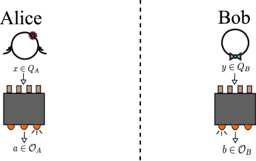
Since we are only concerned with the statistics of the outputs given the inputs, and nothing else matters for us, we can model any such experiment as a black box (see Figure 1.1): which has some buttons as inputs (the possible questions) and a set of light bulbs as outputs (the possible answers to the question). This is called a device-independent scenario, where we do not make any assumption over the internal mechanisms of the devices used for the experiment.
A box is a vector specifying all the joint probability distributions of a particular scenario444For the particular case where Alice and Bob have two possible inputs with two outputs, , is the sixteen-component vector: . In the following sections we are going to analyze which properties the set of boxes satisfies.
In this Chapter we are going to give a brief overview of the concepts and main results in the study of nonlocality. For an introduction to nonlocality, with detailed proofs of many results, the reader is referred to Ref. [Mur12] (only in Portuguese) or Ref. [Qui12]. A nice review, from 2014, contains the references for many important results on the field of nonlocality [BCP+14].
1.1 Local correlations
In the study of nonlocality we are considering a scenario where Alice and Bob are far away from each other during the course of their experiments. We also assume that their choices of which experiment they are going to perform are made when they are already far apart. Our classical intuition leads us to expect that, whichever correlations they observe, they have to be explained by a common cause that does not depend on which experiment they chose to perform (since this choice was made when they were far apart). The boxes that capture this classical intuition are called local boxes.
Definition 1.1.1 (Local correlations).
Local correlations are the ones that can be explained by a local hidden variable model, i.e. a box is local if there exists a variable , independent of the choice of inputs of Alice and Bob, such that
| (1.2) |
where is a probability distribution.
The definition of a local box states that all the correlations observed by Alice and Bob in their experiments are due to the lack of knowledge of some hidden variable . Note that in Definition 1.1.1 we do not make any assumption over the nature of the variable , it can be a continuous variable, it can be a set of variables and so on …The only assumption is that is not correlated with the choices of inputs of Alice and Bob555This assumption is also referred as free will, as, if Alice and Bob can freely make their choices, this assumption will be satisfied. Since here we do not want to make any metaphysical discussion, let us just assume that this independence (between the hidden variable and the choice of inputs) holds, no matter what justifies it. (measurement independence). Another important assumption in Definition 1.1.1 is that, conditioning on all variables that could have a causal relation with a particular event, the probability of this event is independent of any other variable. This is often refereed to as local causality. Therefore for each value of the local probability distribution on Alice’s outcome is independent of Bob’s experiment, i.e. , and the same holds for Bob’s local distribution. This captures the interpretation that the hidden variable would be a common cause in the past that is responsible for generating the correlations.
There are other equivalent ways to formulate Definition 1.1.1, see, for example, Ref. [Fin82]. Moreover, Eq. (1.2) can be derived from a slightly different set of assumptions. But it is important to have in mind that there is always a set of assumptions (measurement independence and local causality in the previous discussion) present in the definition of local correlations, and the violation of a Bell inequality do not tell us which particular assumption is being invalidated. For a very nice discussion on the assumptions implicit in the definition of locality we refer the reader to Ref. [Ara]666This nonlocal reference was added in the revised version of the thesis.. Therefore whenever we use the term nonlocal in this thesis we refer to the impossibility of writing a joint probability distribution in the form of Eq. (1.2).
Definition 1.1.1 reflects the intuition we learn from our daily life experience and it also expresses the predictions of classical theories (as classical mechanics and special relativity), which were the theories that prevailed before the advent of quantum theory.
The local polytope
The set of all boxes that can be written in the form (1.2) is called the local set of correlations, . For any scenario that we consider, i.e. for any finite set of inputs and and any finite set of outputs and , the local set is a polytope. A polytope is a convex set with a finite number of extremal points. The extremal points of the local polytope are the deterministic local boxes:
| (1.3) |
where , is a deterministic probability distribution, and analogously for . One can actually derive that every box that satisfies Eq. (1.2) can be written as a convex combination of deterministic probability distributions, Eq. (1.3)777For this reason Definition 1.1.1 is also called local realism or local determinism..
Proposition 1.1.1 (Local polytope).
The local polytope is the convex hull of the deterministic local boxes:
| (1.4) |
where , , and runs over all possible deterministic boxes of the scenario.
For a scenario with and , the local set is a convex polytope of dimension888The dimension of the polytope is determined by taking into account the normalization of the probability distributions, and the no-signaling condition that we are going to specify soon. with vertices [Pir04].
A convex polytope is fully characterized by its vertices, but an equivalent characterization is given by its facets999This is the Main Theorem for polytopes, see Theorem 1.1 in Ref. [Zie95].. The facets are hyperplanes that delimit the set. The nontrivial facets101010The trivial ones are the positivity condition of the probabilities: . of the local polytope are called tight Bell inequalities [Bel64]. A Bell inequality is a condition that is necessarily satisfied by all local correlations. It can be a tight condition and correspond to a facet of the local polytope, or else it may correspond to faces of the local polytope with lower dimension, or may even not touch the polytope.
In the scenario where Alice and Bob each can chose one between two possible inputs and each input has two possible outputs , the local polytope has as its unique nontrivial facet (up to relabeling of inputs and outputs) the notorious CHSH inequality [CHSH69].
Consider the following expression:
| (1.5) |
where . A substitution of Eq. (1.2) into the RHS of Eq. (1.5) shows that
| (1.6) |
for any local box.
The CHSH inequality (1.6) is the simplest and most well explored of all the Bell inequalities. It was introduced in 1969 by Clauser, Horne, Shimony and Holt [CHSH69]. After the work of Bell [Bel64], which finally opened the possibility to formalize in a mathematical way the concepts of local realism first discussed by Einstein, Podolsky and Rosen [EPR35], the CHSH inequality was proposed as a condition that could be experimentally tested. Inequality (1.6) was used in the first experiment that closed the locality loophole [ADR82], performed by Aspect’s group, and also in the recent groundbreaking loophole-free Bell experiment by Hensen et al.[HBD+15]. A variant of the CHSH inequality (the CH-Eberhard inequality111111The CH-Eberhard inequality is a reformulation of the CHSH inequality which is more suitable for taking into account detection efficiencies. [CH74, Ebe93]) was used in the subsequent experiments by Giustina et al.[GVW+15] and Shalm et al.[SMSC+15]. These last three experiments have finally ruled out local realism in nature121212Up to some stronger loopholes, as the super-determinism, that by definition cannot scientifically be ruled out..
1.2 No-signalling correlations
We may be less picky and not seek a local hidden variable model to explain our correlations, but we want to keep some minimal assumptions about the possible boxes: If Alice and Bob are far away from each other and do not communicate during their experiments, it is reasonable to expect that Bob can get no information about what happens in Alice’s laboratory and vice-versa. This is the no-signaling principle and the most general boxes we are going to deal with are the ones that at least satisfy this constraint. More formally, the no-signaling principle states that the marginals of the local experiments do not depend on the other part’s experiment.
Definition 1.2.1 (No-signaling condition).
A box is no-signaling iff
| (1.7a) | ||||
| (1.7b) | ||||
Note that the no-signaling condition implies that local marginal probabilities are well defined:
| (1.8a) | |||
| (1.8b) | |||
The boxes that satisfy the no-signaling condition (1.7) form the set of no-signaling correlations . is also a convex polytope (as only linear constraints were made to the probability distributions), which contains the classical polytope. This can be easily seen by checking that local boxes (1.2) satisfy the no-signaling condition (1.7), hence
| (1.9) |
Later we are going to see (Section 1.4) that, in general, this inclusion can be a strict relation.
The no-signaling polytope is much easier to characterize than the local polytope since is fully characterized by Eqs. (1.7) (and by the trivial conditions of positivity and normalization of the probability distributions) which are linear constraints that can be easily checked. Although is also delimited by linear constraints, the tight Bell inequalities are not easy to derive and we are left with a description in terms of the deterministic points, which is an integer quadratic problem (see Section 2.2).
1.3 Quantum correlations
Quantum correlations are boxes that can be described as quantum local measurements being performed in a shared quantum state (see Appendix A for an overview of concepts and definitions in quantum theory).
Definition 1.3.1 (Quantum correlation).
A box is quantum if there exist a quantum state and local POVMs and acting on and respectively, such that
| (1.10) |
for arbitrary Hilbert spaces and .
The set of all boxes that admit a description as Eq. (1.10) is the set of quantum correlations . Note that in Definition 1.3.1 we do not put any restriction on the dimension of the system.
The set of quantum correlations contains the local polytope . This is expected by the fact that quantum theory is a generalization of classical theory, hence . Some facts concerning the relation of and are:
-
•
Local measurements in separable quantum states only generate correlations in .
-
•
If the local measurements of one of the parties are jointly measurable131313Two sets of POVMs and are jointly measurable if there exists a third POVM such that for every quantum state . This means that the statistics of the original measurements can be obtained by the marginals of the statistics for the POVM . then the correlations generated are in .
Therefore, in order to observe correlations beyond the classical polytope one necessarily needs entanglement and not joint measurability. Whether these conditions are sufficient to generate nonlocal correlations is a fruitful field of research. In the standard Bell scenario, it is known that some entangled quantum states can only generate classical correlations [Wer89, Bar02] (a systematic method to check whether entangled states admit a local model was recently derived in Refs. [CGRS16, HQV+16]). Partial results concerning joint measurability can be found in Refs. [WPGF09, QBHB16]. More general scenarios were introduced in the study of nonlocality: The hidden nonlocality scenario [Pop95, ZHHH98] where Alice and Bob are allowed to pre-process one copy of their state by a local filtering operation before starting the Bell test; The many-copy scenario where many copies of a state are shared between Alice and Bob [Pal12, CABV13]; And the network scenario [CASA11, CRS12] where copies of a bipartite quantum state are distributed in a network of arbitrary shape and number of parties. These general scenarios were shown to be more powerful than the standard one [HQBB13, CASA11, CRS12] and even the phenomena of super-activation of nonlocality was exhibited [Pal12, CABV13]. However, whether nonlocality, entanglement and not joint measurability are equivalent in these general scenarios remains an open problem.
In Ref. [HM15] we show that the value achieved by a quantum state in a Bell scenario is bounded by a term related to its distinguishability from the set of separable states by means of a restricted class of operations. We also propose quantifiers for the nonlocality of a quantum state in the asymptotic scenarios where many copies and filter operations are allowed, and we show that these quantities can be bounded by the relative entropy of entanglement of the state (or the partially transposed state, in the case of PPT states). A summary of the results of Ref. [HM15] is presented in Appendix B.
Concerning the relation between and , we can straightforwardly verify that quantum correlations satisfy the no-signaling condition (1.7):
| (1.11) | ||||
where is the reduced state of Alice (as defined in (A.5)), and analogously for Bob’s marginal.
In summary, we have
| (1.12) |
and we are going to see in the next Section that all these inclusions can be strict in a general Bell scenario.
Even though the quantum set lies in between two polytopes, in general is not a polytope. The characterization of the quantum set of correlations is the main open problem in the field of nonlocality, and it is not even known for the simplest scenario of two inputs and two outputs141414A partial result characterizes the border of the quantum set in the simplest two-input two-output scenario in the correlation representation [Mas03], i.e. when we consider only the correlators instead of the probabilities .. We know that is a convex set151515It is not hard to show that the convex combination of two quantum boxes can be expressed as a quantum box with measurements and state in a Hilbert space of higher dimension., but it is not known if this set is closed161616A set is closed if every converging sequence of points in converges to a point of .. An alternative way to define the quantum set of correlations is to impose commutativity of every measurement of Alice with every measurement of Bob, in place of the tensor product structure. The set of correlations generated by these assumptions is denoted . It is clear that , and for finite dimensional Hilbert spaces we have equivalence, but whether or not these two sets171717Actually Tsirelson’s statement is concerned with the equivalence of the closure of the sets. are equivalent for the infinite dimensional case is known as the Tsirelson’s problem181818See Tsirelson’s comments on the problem in: http://www.tau.ac.il/~tsirel/Research/bellopalg/main.html. [NCPGV12] (this problem is equivalent to a long standing open problem in -algebra, called the Connes’ embedding conjecture, see [JNP+11]). An infinite hierarchy of well characterized sets that converges to the set , called NPA hierarchy, was introduced by Navascués, Pironio and Acín in Ref. [NPA08] (see more in Section 2.4). This constitutes one of the most powerful tools to deal with problems in the field of quantum nonlocality.
When we are dealing with a particular nonlocality scenario and given a particular Bell expression, as for example , we might be interested in knowing which value can be achieved if Alice and Bob have access to quantum boxes (as we will see later, they can reach ). Due to the lack of characterization of the quantum set of correlations, this is in general a very hard problem. More than that: it is not even known whether the quantum value of a Bell inequality is computable in general, since there is a priori no restriction on the dimension of the Hilbert space for the quantum state and measurements. Only for some particular instances it is possible to compute the value exactly or to find efficient approximations. The NPA hierarchy [NPA08] is typically used to get upper bounds on the quantum bound of Bell expressions. However the quality of approximation achieved by these bounds remains unknown and the number of parameters to be optimized in each level of the hierarchy increases exponentially. Lower bounds are usually obtained by the called see-saw iterative method, where we fix the dimension of the system and recursively optimize over a small set of the variables (the quantum state or one of the party’s measurements) fixing the value of the other variables as obtained in the previous step (see Ref. [WW01b]). Each step of the see-saw is an SDP and can be efficiently solved, however this procedure is not guaranteed to converge not even to the global maximum of the fixed dimension. Hence a central problem of great importance in nonlocality theory is to find easily computable and good bounds to handle general classes of Bell inequalities. In Chapters 5, 6 and 7 we present our contributions in this direction.
1.4 The CHSH scenario
We now illustrate the concepts introduced in the previous Sections exploring the simplest scenario that can exhibit nonlocal correlations: the CHSH scenario [CHSH69]. In the CHSH scenario Alice and Bob each has two possible inputs and each input has two possible outputs .
The local polytope for this scenario can be characterized by the 16 deterministic local boxes or equivalently by its facets. Up to relabel of inputs and outputs the only nontrivial facet of the local polytope is the CHSH inequality Let us write
| (1.13) |
to denote the maximum value attainable by classical (local) theories for the CHSH expression. We have already introduced the CHSH expression in Eq. (1.5) and now we evaluate it for quantum and no-signaling boxes.
In quantum theory, in order to calculate the expected values , we can associate an observable to the measurements of Alice and Bob in the following way
| (1.14) | |||
where are the POVM elements associated to experiment performed by Alice, and analogously for . Hence we have that the correlator is equivalent to the expected value of the operator :
| (1.15) |
Now, consider that Alice and Bob share the maximally entangled singlet state
| (1.16) |
and they perform the measurements associated with the following observables:
| (1.17) |
A direct calculation gives for this experiment.
It was shown by Tsirelson [Cir80] that this is actually the maximum value we can achieve with quantum correlations, hence we have
| (1.18) |
where denotes the maximum value attainable by quantum theory for the CHSH expression.
Now let us consider the following box :
| (1.19) |
All the marginals are well defined and hence this box is no-signaling. However this box is not quantum since one can straightforwardly verify that the value achieved in the CHSH expression is This is actually the maximum possible value (note that the expected values are numbers in the interval ), therefore
| (1.20) |
The box (1.19) was first introduced in Ref. [KT85] and it became well known after the work of Popescu and Rorlich (and hence denoted PR-box) [PR94], where they discussed whether the no-signaling principle was sufficient to limit the nonlocality of quantum theory, showing that actually no-signaling correlations can go far beyond.
So in the simplest nontrivial scenario we have seen that there exist quantum correlations that can violate the locality assumption, hence they cannot be explained by a local hidden variable model. Also we can conclude that the no-signaling principle (1.7) is not enough to set the limits of quantum theory, as it can give rise to correlations much more general than the ones restricted by the quantum formalism. In Chapters 6 and 7 we are going to discuss a bit of the implications of these extremal no-signaling boxes in the scenario of communication complexity.
1.5 Multipartite scenarios
In the study of nonlocality we can also consider scenarios with many parties involved, , all of them performing experiments far away from each other. In these scenarios, our objects of study are the multipartite boxes , where represent the output of part when she/he performs the experiment
The locality condition is straightforwardly generalized for the case of parties:
Definition 1.5.1.
A multipartite box is local if there exists a local hidden variable model that reproduces the correlations, i.e. if there exists a variable , independent of the choice of inputs of the parties, such that
| (1.21) |
where is a probability distribution.
The no-signaling condition is a bit trickier, since now we want to assure no-signaling among all parties.
Definition 1.5.2.
A multipartite box is no-signaling if the no-signaling condition is satisfied by all bi-partition of the parties. More formally, consider a subset of the parties , hence the no-signaling condition states that
| (1.22a) | ||||
for all , , , and all proper subset of the parties, where and , for .
Concerning multipartite nonlocality, we have now different levels of correlations. Analogously to the case of multipartite entanglement (see Appendix A.2.3), where we have the concept of genuine multipartite entanglement (GME), for multipartite Bell scenarios we have the concept of genuine multipartite nonlocality.
Definition 1.5.3.
A -partite box is genuine -partite nonlocal if it cannot be written as
| (1.23) |
for any hidden variables , where and are probability distributions, and runs over all proper subset of the parties. Moreover, each are no-signaling probability distributions191919In the first time the concept of genuine multipartite nonlocality was introduced [Sve87] no assumptions was made about the joint probability distributions. Nowadays, different definitions are considered, see [BBGP13] for a discussion..
Bi-separable quantum states (see Eq. (A.22)) can only generate correlations of the form (1.23), hence if an -partite quantum state exhibits genuine -partite nonlocality, we can conclude that is genuinely -partite entangled. However the converse is not true, and there exist genuinely -partite entangled states that do not exhibit genuine multipartite nonlocality [ADTA15, BFF+16]. In Ref. [Sve87] Svetlichny proposed a method of detecting genuine multipartite nonlocality, designing a tripartite “Bell-like” inequality that was satisfied for all correlations of the form (1.23) but could be violated for genuinely nonlocal correlations. These results were later generalized for multipartite systems in Refs. [CGP+02, SS02]. Other references on the subject are [BBGP13, BBGL11, ACSA10].
Multipartite nonlocality is still poorly explored and the characterization of these scenarios is less known than the bipartite case. In Chapter 7 we are going to present bounds for the quantum value of a particular class of multipartite Bell inequalities and, as an application of these bounds, we present a systematic way to design device independent witnesses of genuine tripartite entanglement.
Chapter 2 A glance at Optimization and Complexity theories
In our daily life we are constantly dealing with constrained optimization problems. As for example, when we go to the cinema with a group of friends. We want to have the best seats (the more central ones in the upper rows of the cinema room, so that we do not have to tilt our heads to watch the movie), but at the same time we want to seat all together, so this is not always an easy problem to solve. And while we choose among the vacant seats, taking into account the pros and cons of the available options and choosing the one that will give a higher gain (which can be accounted by the number of happy people minus the number of unsatisfied people), we are mentally solving this hard optimization problem.
In science the situation is not different and many of the interesting problems can be phrased as an optimization problem. In Chapter 1 we have discussed the concept of nonlocality and how linear expressions (Bell expressions) can be designed to differentiate classical theories (with a local hidden variable model), to quantum theory, and these ones from no-signaling theories. Therefore in the study of nonlocality an important question we recurrently ask is:
Given a Bell expression, what is the maximum value one can achieve if subjected to local/quantum/no-signaling correlations?
The answers to these optimization problems have fundamental importance, since the gaps between the classical and quantum, and the quantum and no-signaling optimal values show an intrinsic difference between these theories. Also these gaps have practical applications for the development of quantum algorithms for information processing tasks.
In this chapter we introduce some concepts and theoretical results in optimization and computational complexity theories.
2.1 Computability and computational complexity
In this Section we present some basic concepts of computability and computational complexity. Our goal is only to give an intuitive idea on the subject. For a formal introduction see [GJ90, AB09] (and also [Kav] for a quick overview).
Uncomputability/Undecidability
Given an problem that we want to solve, the first step in computability theory is to try to design an algorithm which is a systematic way to deal with the problem. For any instance111An instance is a particular input of the problem. In our example of the cinema problem, the problem itself is specified by the parameters: number of people and available seats. A particular instance of the cinema problem is, for example, four people and the two first rows available. (input) of the problem, the algorithm follows a number of specified steps in order to reach the final answer. A problem is said to be computable if there exists an algorithm that, for every input, returns the (approximately) right answer in a finite number of steps.
Definition 2.1.1 (Computability).
A problem (P) is computable if there exists an algorithm such that, for every instance and for every , there exists an integer such that for steps the algorithm returns a value -close222By -close we mean , where is the optimal value and is the value obtained after steps. to the correct value.
In Definition 2.1.1 we consider that the problem might have a continuum of possible answers. For problems with a finite set of possible solutions, -closeness is reduced to exact computation. A very important class of problems with a finite set of solutions are the decision problems. A decision problem is a problem with only two possible answers:“YES” or “NO”.
A remarkable result is that there exist uncomputable/undecidable333Decidability is the term used for the particular case of decision problems. problems, i.e. there exist problems for which it is impossible to construct a single algorithm that for every input will compute the answer in a finite number of steps.
One of the first problems shown to be undecidable was the halting problem. The halting problem is the problem of determining, for a given algorithm and input , whether the algorithm stops (i.e. it gives the output in a finite number of steps), or if it continues running forever. The proof of undecidability was presented by Turing [Tur37] in the same work where he introduced the idea of a universal computing machine: the Turing machine (for a nice presentation and discussion of the halting problem, see [Pen89]).
Computational complexity
Computable problems can be classified according to the amount of resources required to solve them. And by resources we mean time, memory, energy, and so on. The problems are then classified according to the minimum amount of resources required by the best possible algorithm that solves it.
The classes of computational complexity are usually defined in terms of decisions problems. Every optimization problem has a counterpart decision problem associated to it, for example, instead of asking ‘What is the maximum value of a function ?’, we could ask ‘Is the maximum value of greater than ?’. The associated decision problem can be no more difficult than the optimization problem itself (since we could simply solve the optimization problem finding the maximum of and then compare it with ), but interestingly many decision problems can be shown to be no easier than their corresponding optimization problems [GJ90]. Therefore the restriction to decision problems does not lose much generality.
Here we are going to consider the classification of the problems in terms of the time required for the solution of the problem. Given an input of length , the time complexity function of an algorithm, , is the largest amount of time needed by the algorithm to solve a problem with input size . Usually time complexity is expressed in the ‘big O notation’ which describes the limiting behavior of a function. We say if there exists and a constant such that for all .
A problem is considered easy, tractable or feasible if there exists an algorithm that solves the problem using a polynomial in amount of time. In case there is no such polynomial time algorithm, the problem is said to be hard, intractable or infeasible.
The first complexity class we are going to define is the class P, which is the class of problems that can be solved by an algorithm with time complexity polynomial in the size of the input.
Definition 2.1.2 (The complexity class P).
A decision problem belongs to the complexity class P if there exists an algorithm , with time complexity (where is a polynomial in ), such that for any instance of the problem, ,
-
•
if “YES” then “YES”,
-
•
if “NO” then “NO”.
The class P was introduced by Cobham in 1964 [Cob65] and suggested to be a reasonable definition of an efficient algorithm. A similar suggestion was made by Edmonds in Ref. [Edm87]. The belief that the class P constitutes the class of efficiently computable problems444Note that a polynomial time algorithm of complexity seconds would take many orders of magnitude more than the age of the Universe for an input of size 10, while the exponential algorithm of complexity would take only about 17 minutes for the same input size. However the Cobham–Edmonds thesis is supported by many examples of natural problems and how they scale with the input size. Furthermore, polynomial time algorithms involve a deep knowledge of the structure of the problem, in contrast with exponential time algorithms which are usually a mere brute-force search over all possibilities. Here we are just going to assume that the class P is a reasonable definition of efficient (for more discussion on this point, see [AB09, GJ90]). is called the Cobham–Edmonds thesis.
Another important class is the class NP. NP is the class of decision problems that can be efficiently verified555Originally the class NP was defined in terms of non-deterministic Turing machines (a very abstract computational model), and only later it was recognized as the class of problems that can be easily verified (see [Kav])., i.e. once a proof is provided together with the input , one can check in polynomial time whether the answer is “YES”.
Definition 2.1.3 (The complexity class NP).
A decision problem belongs to the complexity class NP if there exists an algorithm , of time complexity (where is a polynomial in ), such that for any instance of the problem , ,
-
•
if “YES” then there is a proof such that “YES”,
-
•
if “NO” then for all proofs “NO”,
It is easy to see that P NP, since for a problem in P one can simply ignore the proof and solve the problem in polynomial time. But whether or not PNP is one of the biggest open problems in computer science.
Complete and hard problems
Many researches believe PNP, based on the fact that some problems in NP seems to be intrinsically more difficult than the problems in P. However up to now no formal proof in any direction was ever found. An intermediate advance in the classification of NP problems was made by the introduction of the concept of a polynomial time reduction, which allowed to select the hardest problems of the class NP. These hardest problems are the ones for which it is most unlikely to find an efficient algorithm, and in case PNP these problems definitely belong to the non-intersecting region.
Definition 2.1.4 (Polynomial time reduction).
A problem is polynomial time reducible to , if there exists a polynomial time algorithm such that for every input of problem
| (2.1) |
and in this case we say .
The idea of a reduction is to map a problem into another problem , such that by solving one is able to get the solution of . However, since we are concerned with efficiency, a good reduction is one that can be performed in polynomial time. With that in mind, by Definition 2.1.4 we see that if problem is efficiently solvable then is also efficiently solvable666We simply have to apply the reduction algorithm which takes polynomial time, and then we solve which also takes polynomial time.. And if is not efficiently solvable, we can conclude that cannot be efficiently solvable, otherwise we would have a contradiction. Therefore if , then we can say that is at least as hard as .
Definition 2.1.5 (NP-hard problems).
A problem is NP-hard if there exists a polynomial time reduction of every problem NP to problem :
| (2.2) |
Definition 2.1.6 (NP-complete problems).
A problem is NP-complete if is NP-hard and if NP.
The NP-complete problems are the hardest problems of the NP class, since by finding a polynomial time algorithm for solving an NP-complete problem one automatically solves any problem in NP in polynomial time (and then would have proved PNP!).
Note that once we identify an NP-complete problem , by reducing it to an NP problem , we automatically prove that is also NP-complete. Hence the concept of reduction opens the possibility of many proofs of hardness in the field of computational complexity. The first proof of NP-completeness was given by Stephen Cook in Ref. [Coo71], where he showed that the SAT problem777The SAT (satisfiability problem) is the problem of determining whether there exists a consistent assignment for the variables of a particular Boolean circuit such that the whole expression is evaluated as true. For example, the Boolean circuit can be evaluated as true with the assignment true, false, and true. is NP-complete (known as the Cook-Levin theorem[Coo71, Lev73]).
In Ref. [Kar72], Richard Karp uses Cook-Levin theorem in order to show that there is a polynomial reduction from the SAT problem to each of 21 combinatorial and graph theoretical computational problems. In particular a -integer programming and the calculus of the independence number of a graph (that we are going to discuss later) are NP-complete problems.
2.2 Optimization problems
In the previous Section we presented the concepts of computability and uncomputability. Also, we have seen that the computable problems can be divided in classes of complexity which classify the problems according to how many resources are necessary to solve it. In this section we discuss a bit of the theory of optimization following approaches of Refs. [BTN13] and [BV04].
Let us consider an optimization problem where we want to minimize a function subjected to some constraints:
| (2.3) |
where
-
•
is the optimization variable,
-
•
is an -variable real function called objective function,
-
•
are -variable real functions called constraint functions.
The set of points for which the objective and constraint functions are defined is called the domain of the problem :
| (2.4) |
A point is feasible if it satisfy all the constraints, i.e. and . The set of all feasible points is called the feasible set ,
| (2.5) |
The optimal value of problem is the infimum of over the feasible points
| (2.6) |
If the optimal value is achieved by a feasible point then the problem is said to be solvable. However, for some problems the optimal value may not be achieved by any feasible point.
The simplest optimization problem is the linear programming (LP) where the objective and constraints are affine functions888A function is affine if .. For an LP the numerical method of interior-point999For details of the interior-point method see Ref. [BV04]., developed in the 1980s, can solve it efficiently with operations, where is the number of variables and the number of inequality constraints. Therefore LP P.
Many advances in numerical methods for solving optimization problems are due to the recognition that the interior-point method can also be used to solve other convex optimization problems efficiently. Convex optimization problems are the ones where the objective and constraint functions are convex101010A function is convex if , .. Hence a convex optimization problem is usually considered a tractable one, whereas non-convex problems are in general hard. Fortunately many interesting problems in many areas: physics, mathematics, engineering and so on, can be phrased as a convex optimization problem.
A particular case of convex optimization problem is the semidefinite programming (SDP). For SDPs, algorithms which utilize the method of interior-point are well established, therefore, these problems can also be solved efficiently (in polynomial time in the number of variables). For more general convex problems the numerical methods are not so well established as for LP and SDP, still the interior-point methods work well in practice.
As nicely pointed by Boyd and Vandenberghe [BV04] these numerical methods for solving these problems are so well structured that they can be considered a technology:
“Solving [LP and SDP] is a technology that can be reliably used by many people who do not know, and do not need to know, the details.”
In this Section, we present the formal definitions of linear programming (LP), semidefinite programming (SDP), and integer programming (IP).
Linear optimization
A linear programming (LP) is an optimization problem (2.3) where the objective and constraint functions are affine. An LP can be expressed as
| (2.7) |
where all the constraint functions are expressed in a unique vector inequality111111And remember that an equality constraint can always be expressed as two inequality constraints: and . , , which represents a component-wise relation . , , , and is a matrix. We are making use of Dirac’s notation121212The called “braket” notation, used in quantum theory, was introduced by Dirac in Ref. [Dir39]. for consistency with the other chapters.
Semi-definite programming
In order to generalize an LP one can relax the linearity condition of the objective or the constraint functions. However another way to generalize an LP that leads to a class of very interesting problems is to keep the objective and constraint functions linear but to relax the meaning of in the inequality constraints.
The order relation in an LP, Eq. (2.7), is a coordinate-wise relation where and satisfy
| (2.8) |
However a partial order relation can be defined in a more general framework. A good partial ordering is completely determined by a subset , of a vector space , where the relation is defined as:
| (2.9) |
and determines the set of positive elements:
| (2.10) |
In order to satisfy some expected properties (see [BTN13] for more details) the set cannot be arbitrary and it has to be a pointed cone, i.e.
-
(i)
is nonempty and closed under addition: .
-
(ii)
is a conic set: .
-
(iii)
is pointed: and .
An optimization problem whose constraints are defined by the partial ordering , for a set satisfying properties (i)-(iii), is called a conic problem.
Now let be the cone of symmetric positive semidefinite matrices , this defines a semidefinite programming (SDP):
| (2.11) |
where is a linear map from vectors in to the space of symmetric matrices . , and and are vectors in .
The standard form of an SDP (and the one we are going to deal with in the following chapters) is
| (2.12) |
where .
The formulations (2.11) and (2.12) are equivalent, and a problem in form (2.11) can always be rephrased into the from (2.12) and vice-versa[BV04].
From now on we are going to omit the subscript in the ordering relation , but from the context it will be clear which ordering relation is being applied.
Integer programming
An integer programming (or integer linear programming) is a problem where the objective and constraint functions are affine functions but the variables are restricted to be integers131313 This restriction can be seen as a non-linear constraint, for example, if is restricted to assume values , this is equivalent to require the quadratic constraint to be satisfied.. -integer programming is the particular case of integer programming where the variables are restricted to assume the values 0 or 1. A general -integer programming (IP) can be written as
| (2.13) |
where and is an real matrix.
Problems of the form (2.13) appear in the study of nonlocality, in the calculus of the classical value of a Bell expression. Note that a Bell expression is a linear function of the joint probability distributions , and one can easily check that imposing no-signaling constraints (which are linear constraints) together with determinism, i.e. , is equivalent to impose deterministic locality: . Consequently, the search over all deterministic local boxes, which is sufficient to obtain the classical value of a Bell expression (see Chapter 1), is a -integer programming.
As previously mentioned, -integer programming was shown to be an NP-complete problem [Kar72], therefore the task of obtaining the classical value of a Bell inequality is hard in general.
2.3 Duality
The idea of the dual of a problem is to play with the constraint inequalities (summing equations, adding trivial inequalities and so on) in order to obtain a quantity that is always smaller then the optimal value of problem . In this Section we will study the theory of Lagrange duality [BV04].
Given an optimization problem :
| (2.14) |
the Lagrangian function, , is defined as
| (2.15) |
where and . Note that if , for every feasible point of we have .
Now we define the dual function, as
| (2.16) |
The dual function is the point-wise infimum of a family of affine functions of the variables , and hence is always concave141414A point-wise infimum of an affine function over variable can in general be written as . Now, taking , we have even though no structure was assumed about the problem .
Let be the optimal solution of the problem . By construction we have that
| (2.17) |
And therefore is always a lower bound to the value of problem . One can then look for the best lower bound that can be obtained from , and that is the idea of the Lagrange dual problem :
| (2.18) |
Note that the Lagrange dual problem is the maximization of a concave function subjected to linear constraints. The maximization of is equivalent to the minimization of , which is then a convex function. Therefore is a convex optimization problems.
Theorem 2.3.1 (Weak duality).
Let be the optimal value of a problem , and be the corresponding Lagrange dual problem with optimal value . It holds that
| (2.19) |
Where is the duality gap.
The Weak duality Theorem follows by construction of the dual problem. Weak duality holds in general for any kind of optimization problem, as no restriction on the nature of the objective and constraint functions was made for the construction of the Lagrangean. However for many convex problems an even stronger result holds, that the optimal value of the dual is actually equal to the optimal value of the problem . This is stated by Slater’s condition.
Theorem 2.3.2 (Strong duality- Slater’s condition).
Given a convex optimization problem of the form
| (2.20) |
where is a convex function bounded below and are -convex functions151515A function is -convex if , for . . If there exists a strictly feasible point161616A point belongs to the relative interior of a set , if (2.21) where .
| (2.22) |
then .
There are other results which establishes conditions for strong duality for non-convex problems. These conditions are in general called constraint qualifications [BV04].
2.4 SDP relaxations of hard problems
The idea of a relaxation is the following: In an optimization problem we want to find the optimum value of a function searching over the domain , which is determined by the constraints of the problem. However even when the function is simple (a linear function for example), it might be the case (and it is the case in many interesting problems) that the domain is extremely hard to characterize. An alternative way to deal with this difficulty is to consider the problem , where, instead of searching for the minimum of over the set , we make the search over a bigger (relaxed) set (see Figure 2.1), , which is simpler to describe.
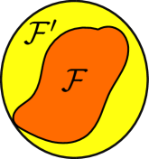
Since , the optimal value obtained for problem is smaller than or equal the optimal value obtained for problem . Hence a relaxation is a way to get lower bounds for an optimization problem .
A relaxation is wanted to satisfy two features: it should be efficiently solvable (i.e. the relaxed set has to be nicely characterized), and at the same time it should be good meaning that the value obtained in the relaxation is close to the actual value (we do not want a relaxation that gives a completely non-informative result).
As an example let us consider the problem of finding the independence number of a graph 171717The independence number of a graph is the maximum number of vertices such that no two of each are connected by an edge (see Chapter 4). with vertices, which can be formulated as the following -integer programming:
| (2.23) |
As we have argued before, this is an NP-complete problem and hence considered intractable for large . A simple relaxation can be derived by just turning the nonlinear constraint into a linear one
| (2.24) |
We have that for every graph , since we now allow to assume all the values between 0 and 1. Moreover, problem (2.24) is a linear program which can be efficiently solved.
For a long time the only known practical relaxations were the LP ones. However, with the advent, over the last decades, of techniques for efficiently solving semidefinite programs, it came the possibility of exploring semidefinite relaxations, which has become a fruitful area of research181818For a detailed discussion see the Preface of Ref. [BTN13].. Semidefinite relaxations have been shown to be particularly useful for combinatorial problems. We are going to see, in Section 4.1, an SDP relaxation for the independence number problem (2.23) (the Lovász number).
NPA hierarchy
We have stated that calculating the classical value of a Bell inequality is a -integer programming, and thus it is NP-hard. For the quantum value the situation is even worse! Note that in Chapter 1, when we define the quantum boxes, we make no restriction over the dimension of the system, and hence to obtain the quantum value one should optimize over all possible states and measurements in all possible dimensions. There is no known algorithm to determine the quantum value of a general Bell inequality191919We are going to see in Chapter 3 that for a particular class of Bell inequalities, the xor games, the quantum value can be determined efficiently by an SDP. in a finite number of steps and therefore this problem may even be uncomputable (In Ref. [AFLS15] the authors conjecture that it is actually non-computable.).
The most general method known to deal with this intractable problem was introduced by Navascués, Pironio and Acín, in Ref. [NPA08]: the NPA hierarchy. The NPA hierarchy is a hierarchy of semidefinite programs where each level corresponds to an optimization over a tighter relaxation of the quantum set of correlations. These sets are nicely constrained by a relation and therefore calculating the optimal value of a Bell inequality over a level of the hierarchy is a semidefinite program. The hierarchy is proved to converge to the set which is defined as following:
Definition 2.4.1.
The set is the set of boxes such that
| (2.25) |
for some state and projective measurements202020Since we do not fix dimension, there is no loss of generality in restrict to pure states and projective measurements. This is due to Naimark’s Theorem, see https://cs.uwaterloo.ca/~watrous/CS766/LectureNotes/05. and , acting on , satisfying
| (2.26) |
Note that the set of quantum correlations is contained in , since all local measurements of Alice commutes with local measurements of Bob. But whether or not is an open problem known as Tsirelson’s problem [NCPGV12] (see discussion in Section 1.3).
The NPA hierarchy constitutes one of the most powerful tools in the field of nonlocality, and it has led to the derivation of innumerous results. However the quality of the approximation achieved by these bounds remains unknown in general. Moreover for a Bell inequality with inputs and outputs per party, the -th level of the hierarchy involves a matrix of size as an SDP variable, so, in general, the complexity increases exponentially with the level of the hierarchy.
Chapter 3 Nonlocal games
Some Bell inequalities can be naturally phrased in the framework of a game. A nonlocal game is a cooperative task where the players receive questions from a referee and they are supposed to give answers in order to maximize some previously defined payoff function. Upon starting the game, the players are not allowed to communicate anymore, therefore any strategy has to be agreed in advance.
Nonlocal games have a wide range of applications. They play an important role in the study of communication complexity [BCMdW10, BZPZ04] (and vice-versa) and in the formulation of device-independent cryptographic protocols [Eke91, CR12].
In a computer science language, a nonlocal game with players can be seen as the particular case of multiprover interactive proof systems with provers and one round. An interactive proof system consists of an all powerful111Powerful in a computational sense, meaning that the prover has unbounded resources, although only classical resources, and unlimited computational power., but untrusted, prover who wants to convince a verifier, who has limited computational power, of the truth of some statement by exchanging messages in many rounds. A multiprover interactive proof system is an interactive proof system with many provers, who may be bounded not to communicate during the proof. Multiprover interactive proof systems were introduced in Ref. [BOGKW88] as an alternative to allow for the performance of some cryptographic tasks without relying on extra assumptions, such as the existence of one-way functions222A one-way function is a function that can be computed in polynomial time for any input , however the function is hard to invert. The existence of one-way functions would imply that PNP. or limitations on the computational power. With the introduction of many provers these extra assumptions can be replaced by the condition of physical separation of the provers during the course of the protocols. For further remarks on the connection of interactive proof systems with entangled provers and the quantum value of nonlocal games see Ref. [CHTW04].
In this chapter we present definitions and results on nonlocal games. In the first sections we restrict the presentation to the case of -player games. The case of -player games is discussed in Section 3.4. For a nice introduction to nonlocal games see Ref. [CHTW04].
3.1 Definitions
Definition 3.1.1 (Nonlocal Game).
A nonlocal game is a cooperative task where players, Alice and Bob, who are not allowed to communicate after the game starts, receive respectively questions and , chosen from a probability distribution by a referee. Upon receiving the questions, Alice is supposed to give an answer and Bob . The winning condition of the game is defined by the payoff function which assumes value to indicate when the players win and value to indicate when they lose.
Given a particular strategy applied by the players, which is specified by a box , the figure of merit that we are interested in analyzing is the average probability of success given by
| (3.1) |
Note that can be regarded as a Bell expression, since it is a linear function of the joint probability distributions .
Classical strategies
The maximum average probability of success optimizing over all possible classical strategy is the classical value of the game, denote . In order to obtain we have to optimize over the local boxes of the particular Bell scenario defined by the game. As we argued before, the maximum value of is attained by a deterministic strategy, hence:
| (3.2) |
where and are deterministic probability distributions. The number of possible deterministic strategies for a particular game is , which increases exponentially with the number of inputs.
Quantum strategies
A general quantum strategy is described by the players sharing a bipartite quantum state of arbitrary dimension and giving their answers according to the result of local measurements, and , that they perform in their systems:
| (3.3) |
Since we do not make any restriction on the Hilbert space dimension of the system we can actually restrict ourselves to pure states and projective measurements333It is a consequence of Naimark’s Theorem that an arbitrary POVM on a system of Hilbert space is equivalent to a global projective measurement in , where is the Hilbert space of an auxiliary system. See https://cs.uwaterloo.ca/~watrous/CS766/LectureNotes/05.. Therefore, the quantum value of the game, , which is the maximum average probability of success of players applying a quantum strategy, is given by:
| (3.4) |
where , for arbitrary Hilbert spaces and , and and are projective measurements.
As discussed before, we do not put any restriction on the dimension of the system and, as a particular class of Bell inequalities, it is not known if the quantum value of a nonlocal game is computable in general (see Section 2.4).
No-signaling strategies
We also define the no-signaling value of the game, denoted
| (3.5) |
The no-signaling value is easily calculated by a linear programming, since we have a linear function of the variables , subjected to linear constraints given by the no-signaling conditions (1.7).
3.2 xor games
In this Section we focus on the so-called xor games, introduced in Ref. [CHTW04]. xor games are the simplest class of nonlocal games where the players have two possible answers, , and the payoff function only depends on the sum modulo two444The sum modulo 2 is equivalent to the logical operation exclusive or, also denoted xor, that is the reason for the name of the games. of their outputs:
| (3.6) |
for some function .
Definition 3.2.1 (xor games).
An xor game, is a nonlocal game where Alice and Bob receive respectively questions and , chosen from a probability distribution by a referee. Upon receiving the questions, Alice outputs a bit and Bob outputs bit . The players win the game if .
The average probability of success (3.1) for an xor game can be written as555Where we have used the fact that (3.7)
| (3.8) |
The first on the RHS of Eq. (3.8) can be interpreted as the probability of success of the players when they apply a totally random strategy (i.e. if upon receiving her input Alice tosses a coin to determine her output , and Bob does the same).
The bias of the game represents how much a particular strategy is better (or worse) than the completely random strategy, and is defined as:
| (3.9) | ||||
In expression (3.8) we see that is related to the expected value of binary observables (see Eq. (1.15)), . Therefore xor games are equivalent to the important class of Bell expressions that involve only terms with correlators , the full-correlation Bell inequalities, which is a widely studied class of Bell inequalities [Weh06, WW01a]. The CHSH inequality (1.5) being the most remarkable example of a full-correlation Bell inequality.
The game matrix
To every xor game we can associate a matrix, the game matrix , which carries all the information necessary to describe the game: the inputs’ probability distribution and the winning condition specified by :
| (3.10) |
where and define orthonormal basis and and run over the inputs of Alice and Bob respectively.
SDP characterization of the quantum value of an xor game
For the particular class of bipartite xor games, a theorem due to Tsirelson [Tsi80, Tsi87], leads to the result that the quantum value of these games can be computed efficiently by a semidefine program [CHTW04, Weh06].
Theorem 3.2.1 (Tsirelson [Tsi80]).
Let and be observables with eigenvalues in the interval acting on and respectively. Then, for any state , there exist unit vectors such that
| (3.11) |
Conversely, let , be unit vectors. Then, for the maximally entangled state , with , , there exist -observables, acting on and acting on , such that
| (3.12) |
Tsirelson’s Theorem establishes a one-to-one relation between quantum strategies and the inner product of real vectors.
From now on let us set and . The optimal quantum strategy of an xor game is given, in general, by Alice and Bob measuring observables and on a shared pure quantum state of arbitrary dimension. By Tsirelson’s theorem 3.2.1 the expected value of these observables can be replaced by the inner product of unit vectors in . This implies that calculating the quantum value of an xor game can be formulated as a semidefinite program [Weh06].
Theorem 3.2.2.
The optimal quantum bias, , of an xor game with game matrix is given by
| (3.13) |
where is a vector whose entries are the diagonal elements of matrix , is the all 1’s vector, and . is the strategy matrix defined as . The matrices with and represent local terms.
Proof.
Let us consider an xor game with questions for Alice, questions for Bob, associated game matrix , and winning condition determined by function . We have that
| (3.14) |
and for a quantum strategy where Alice and Bob perform the measurements and , respectively, in a quantum state
| (3.15) |
where and are defined as in Eq. (1.14). Hence
| (3.16) |
Now we can define the vectors
| (3.17) | ||||
so that
| (3.18) |
Let
| (3.19) |
be the strategy matrix that represents this particular strategy. Together with the game matrix given by Eq. (3.10) we have that
| (3.20) |
Now let us define the matrix whose columns are composed by the vectors and :
| (3.21) |
and set . is the so-called Gram matrix of the set of vectors , and . Note that if the vectors are normalized, all the diagonal elements of are equal to 1. By defining we have
| (3.22) |
Finally, we use the fact that iff it is the Gram matrix of a set of vectors [HJ12], in order to guarantee that, for every feasible in problem , there exist a set of normalized vectors , , for some . And by Tsirelson’s theorem 3.2.1, each solution can then be described by -observables applied to a quantum state . Which ends the proof. ∎
For a classical deterministic strategy, all vectors and are equal to , for a single unit vector , since the expected values assume values . The strategy matrix of a classical deterministic strategy is thus a matrix with entries with all columns (and rows) being proportional to each other.
An upper bound to the quantum value of xor games
We now show that the quantum value of an xor game can be upper bounded by a quantity related to the spectral norm of the game matrix .
Theorem 3.2.3.
Given a bipartite xor-game, with inputs for Alice, inputs for Bob, and an associated game matrix , the quantum value is upper bounded by
| (3.23) |
where is the maximum singular value, or the spectral norm, of the matrix .
Proof.
We follow the approach of Ref. [LPSW07]. Given a bipartite xor-game, , its quantum value is given by
| (3.24) |
Note that we have replaced the supremum of Eq. (3.4) by a maximum, since Tsirelson’s Theorem 3.2.1 guarantees that the optimal quantum value for xor games is always achieved by a quantum strategy (and even more, that this strategy involves a finite dimensional system).
Now let be the quantum state and observables corresponding to the optimal strategy for the game , and let us define the unit vectors
| (3.25a) | ||||
| (3.25b) | ||||
So that we have
| (3.26) | ||||
∎
The bound (3.23) was also derived and studied in details in Ref. [EKB13], where the authors provide necessary and sufficient conditions for the bound to be tight. For the case of , Theorem 3.2.3 can be derived from the dual of problem (3.13). One can show that is a feasible solution to the dual problem , and hence, by the weak duality theorem 2.3.1, it is an upper bound on the quantum bias [Weh06] (see Appendix E.1).
No-signaling value of an xor game
An xor-game can always be won with certainty by a no-signaling strategy, i.e. .
In order to see that, consider the strategy defined by
| (3.27) |
This strategy is no-signaling, because all the marginals are uniform
| (3.28) |
and by construction it wins the game with certainty. The no-signaling boxes defined by Eq. (3.27) are the generalization of the PR-boxes (Eq. (1.19)), introduced in Chapter 1, for the case of more inputs per party.
3.3 Linear games
Another class of games that we are going to consider are the called linear games. They are a generalization of xor games to a larger alphabet output size. Linear games constitute a particular case of a more general class of nonlocal games, the unique games.
Unique games have been extensively used in the study of hardness of approximation of some NP-complete problems, in attempts to identify the existence of polynomial time algorithms to approximate the optimal solution of the problem to within a constant factor [Hås01, KKMO07]. Unique games is the class of nonlocal games where for each pair of questions, , there is an associated permutation and the players win the game iff Bob’s output corresponds to the permutation of Alice’s output. Linear games constitute the particular case of unique games where all the associated permutations commute and therefore it can be defined in terms of an Abelian group .
Definition 3.3.1.
A two-player linear game is a nonlocal game where two players Alice and Bob receive questions , from sets and respectively, chosen from a probability distribution by a referee. They reply with respective answers where is a finite Abelian group with associated operation . The winning condition of the game is defined by a function , such that if and 0 otherwise.
Some concepts and formal definitions on groups are stated in Appendix C.
The average probability of success of the players in a linear game can be written as
| (3.29) |
An xor game can be seen as a linear game with . We can also define the generalized xor games, xor- games, denoted , as the class of linear games associated to the cyclic group (the set with the operation of addition modulo ).
Perfect no-signaling strategy for linear games
The existence of a perfect no-signaling strategy that wins the game with probability 1 also holds for linear games. For every linear game there exist a no-signaling strategy that perfectly wins the game:
| (3.30) |
Such a strategy is defined as
| (3.31) |
The strategy (3.31) clearly wins the game, and also it is no-signaling since all the marginals are fully random:
| (3.32) |
and analogously for .
3.4 -player games
In this Section we present the generalization of the previous definitions for games with players.
Definition 3.4.1 (-player nonlocal Game).
An -player nonlocal game is a cooperative task where players , who are not allowed to communicate after the game starts, receive respectively questions , where , chosen from a probability distribution by a referee. Upon receiving question player is supposed to answer . The winning condition of the game is defined by a payoff function which assumes value to indicate when the players win and value to indicate when they lose.
The probability of success of the players for a particular strategy defined by the box is given by
| (3.33) |
where denotes the input string, and analogously for and .
The definition of linear games can be straightforwardly generalized for an -player game in the following way:
Definition 3.4.2.
An -player linear game is a nonlocal game where the players answer with , where is a finite Abelian group with associated operation , and the predicate function only depends on the sum of the players outputs:
| (3.34) |
for .
The probability of success of a particular strategy in a -player linear game is given by
| (3.35) |
The classical value of an -player game
The classical value of an -player nonlocal game is obtained by an optimization over deterministic local strategies
| (3.36) |
where represents a deterministic probability distribution.
The number of possible deterministic strategies also increases exponentially with the number of parties. For a game with players, questions per player and outputs per question, the number of deterministic strategies is .
The quantum value of an -player game
A general -partite quantum strategy can be described by the players sharing an -partite pure state of arbitrary dimension and performing local measurements on it. The quantum value of the -player game is then given by
| (3.37) |
The case of multiplayer games is even more challenging than the bipartite case. For bipartite XOR games, we have seen that Tsirelson’s theorem (Theorem 3.2.1) guarantees that the best performance of quantum players can be calculated exactly and efficiently using a semidefinite program, Eq. (3.13). For three players, even for the case of xor games the quantum value is known to be NP-hard666In terms of the number of possible questions. to approximate [Vid13].
In chapter 5 we deal with bipartite xor games and present results of Ref. [RKMH14] concerning games with no-quantum advantage and results on the Shannon capacity of xor-game graphs. In Chapter 6 we provide an upper bound to the quantum value of a 2-player linear game and present results of Ref. [RAM16]. In Chapter 7 we generalize the results for -player linear games presenting the results of Ref. [MRMT16].
Chapter 4 Graph theoretic approach to nonlocality
The graph theoretic approach to quantum correlations was introduced by Cabello, Severini and Winter [CSW10, CSW14] in the framework of contextuality scenarios111In a contextuality scenario we do not necessarily have parties. The hypothesis in question is whether an observable that belongs to two different sets of mutually commuting observables, called the contexts, and , can have a description independent of the context. In a Bell scenario the commutation of observables that form each context is guaranteed by the tensor product structure of the parties’ experiments., where Bell scenarios can be seen as a particular case of it. Further refinements to the particular case of nonlocality scenarios where made in Refs. [AFLS15, CMSS14, RDLT+14]. In this chapter, we will see how the classical, quantum, and no-signaling values of a Bell expression can be associated to graph parameters.
4.1 A bit of zero-error information theory
In 1956 Shannon [Sha56] studied the concept of zero-error capacity of a communication channel. The zero-error capacity is defined as the maximum rate at which it is possible to transmit information with zero probability of error through a channel .
A channel is described by a set of input letters , a set of output letters , and the transition probabilities that represents the probability that an input will generate an output . In the analysis of zero-error capacity we are not interested in the particular values of the transition probabilities but only whether they are zero or not. In order to deal with the important properties of the zero-error capacity , we can associate a graph to the channel in consideration.
Definition 4.1.1 (Confusability Graph).
The confusability graph associated to a channel is a graph where each input letter of the channel corresponds to a vertex
| (4.1) |
and there is an edge connecting two vertices and if these inputs can be confused by the channel
| (4.2) |
An alternative quantity that carries all the information contained in the graph is the adjacency matrix.
Definition 4.1.2 (Adjacency Matrix).
The adjacency matrix associated to a graph is defined as
| (4.3) |
The maximal number of 1-letter messages, , which can be sent through a channel without confusion can be extracted directly from a graph invariant. A bit of thinking222Or maybe a few bits. But note that since the independence number picks the maximum number of vertices such that no two of which are adjacent, this represents the maximum number of letters such that none of them can be confused. leads us to conclude that is equal to the independence number of the confusability graph :
| (4.4) |
The independence number of a graph is the cardinality of the maximal independent set, which is a subset of vertices such that none of which are adjacent . It is described by the optimization problem (2.23).
Formally, the zero-error capacity is defined as
| (4.5) |
where is the largest number of -letter messages that can be sent through the channel without confusion. The number of non-confusable -letter messages is given by the independence number of the graph :
| (4.6) |
where denotes the strong product of graph with itself times.
Definition 4.1.3.
The strong product of graphs and is such that
-
•
,
-
•
and .
In terms of a channel , Definition 4.1.3 captures the idea that two 2-letter words are confusable if they are confusable in the first and in the second letter.
So we have that
| (4.7) |
where
| (4.8) |
From now on we refer to as the Shannon capacity of graph333The supremum in Eq. (4.5) can actually be replaced by a limit, since the strong product satisfies (4.9) which can be proved by noting that given an independent set of graph , one can generate an independent set for by taking . .
As an example let us consider the channel with confusability graph given by the pentagon :
![[Uncaptioned image]](/html/1704.04922/assets/x3.png)
The maximum number of 1-letter messages we could send through this channel without confusion is 2, and we have . We could for example send letter or . Now, considering 2-letter messages, we could obviously make the four non-confusable words: , and . However one can check that the following five words of size two: , are such that no two of them can be confused, and actually . Therefore, we conclude that .
In contrast to the ordinary channel capacity where a vanishing probability of error is allowed [Sha48] and the capacity can be efficiently calculate, it is not know whether the zero-error capacity is computable. By the definition given in Eq. (4.8), we have a supremum over and at the moment there is no algorithm to decide the value of in a finite number of steps for an arbitrary graph.
In 1979 Lovász [Lov79] introduced an efficiently computable upper bound to the Shannon capacity (and therefore also for the independence number ). The Lovász number is a graph invariant defined as follows:
Definition 4.1.4 (Lovász Number).
Consider an -vertex graph . Let the set of vectors be an orthonormal representation of and be a unit vector. The Lovász number is given by
| (4.10) |
An orthonormal representation of the complementary graph is a set of real vectors associated to the vertices of graph such that and .
By calculating , Lovász proved [Lov79] that the previously known lower bound for the Shannon capacity of the pentagon, , is actually the exact value: .
There are many equivalent characterizations of the Lovász number [Lov09, Knu94], here we consider one that will be useful in Chapter 5:
Theorem 4.1.1 ([Lov79]).
Given a graph , consider the family of symmetric matrices such that
| (4.11) |
The Lovász number is the minimum of the maximum eigenvalue of such matrices:
| (4.12) |
Theorem 4.1.1 can be formulated as the semidefinite program :
| (4.13) |
where imposes that is greater than or equal to the maximum eigenvalue of a symmetric matrix satisfying (4.11), and the minimization picks the smallest of the maximum eigenvalues. Characterization (4.13) makes it clear (see Section 2.2) that the Lovász number can be efficiently determined.
4.2 The exclusivity graph
The graph theoretic approach to contextuality and nonlocality, that we call CSW approach, was first introduced in Ref.[CSW10] (and published later in Ref. [CSW14]). The idea is to associate with a given Bell scenario a graph called the exclusivity graph. The exclusivity graph has the vertices labeled by the events444By event we denote the occurrence of Alice measuring and obtaining outcome , and Bob measuring and obtaining outcome . of the particular Bell scenario , and the edges connect vertices which correspond to exclusive events (e.g., Alice measuring and obtaining is exclusive with any event where Alice measures the same and obtains ). The idea of the CSW approach is to take into account that the probabilities of exclusive events should sum up to no more than one.
Definition 4.2.1 (Exclusivity graph).
The exclusivity graph associated to a Bell scenario is a graph with vertices representing the possible events: , and adjacencies defined by
| (4.14) |
where and denotes respectively the logical operations AND and OR.
Given a Bell scenario with boxes , we denote a Bell expression by such that its value for a particular box is given by . Note that every Bell expression can be written with non-negative coefficients only555One just has to use the normalization condition of probability distributions, , in order to avoid the negative coefficients., .
Now, given a Bell expression with positive coefficients , we can consider the weighted exclusivity graph , where the weight is attributed to each vertex of the exclusivity graph . What is shown in the CSW approach [CSW14] is that the local, quantum and no-signaling values of a Bell expression , respectively , , and , are related with invariants of the associated weighted exclusivity graph.
Theorem 4.2.1 ([CSW14]).
Given a Bell expression , and the weighted exclusivity graph , it holds that
| (4.15) |
where , , and are respectively the weighted independence number, the weighted Lovász number, and the weighted fractional packing number.
The graph invariants that appear in Theorem 4.2.1 are defined bellow.
Definition 4.2.2.
The weighted version of the independence number , the Lovász number , and the fractional packing number of the weighted graph are defined by the following optimization problems:
| (4.16) |
| (4.17) |
| (4.18) |
In order to understand Theorem 4.2.1, note that the weighted independence number (4.16) captures the idea that a deterministic probability is associated to vertex , and therefore gives the classical value of a Bell inequality . Concerning the Lovász number (4.17), the term can be interpreted as the probability resultant of a projective measurement (determined by the vector ) in the quantum state . However note that no tensor product structure was imposed for these measurements and state, which justifies the upper bound . For the fractional packing number (4.18), the constraint that for all clique666A clique in the graph is a subset of vertices such that every two vertices in are adjacent. captures the no-signaling conditions (1.7) and normalization of the probabilities (), and therefore it justifies .
The weighted Lovász number (4.17) was introduced and studied in Ref. [Knu94], and it also admits an SDP characterization. The weighted independence number (4.16) is a -integer program which is in general NP-complete, and the weighted fractional packing number777The fractional packing number is easy to determine once the cliques of the graph are known, however if this is not the case, the problem of finding the cliques of a graph is also NP-complete. (4.18) is defined by an LP.
The CSW approach had great impact in the field of nonlocality and contextuality, allowing us to use techniques of combinatorics to derive many results in these fields (see for example [ATC14, CMSS14] and references therein). The CSW approach was further refined in Ref. [AFLS15] where the authors consider hypergraphs from which it is possible to extract information about the complete nonlocality/contextuality scenario, and not only about the Bell inequalities.
For contextuality it holds that given an exclusivity graph there always exists a contextuality scenario and an inequality whose quantum value is equal to the Lovász number of the graph . This can be seen by the definition (4.10), where one can interpret the vectors as projective measurements being performed on the quantum state . However for nonlocality, equality does not hold in general since the tensor product structure is not captured by the Lovász number. In Ref. [RDLT+14] the authors introduce the exclusivity multigraph with the aim to capture the structure presented in the nonlocality scenario. In the exclusivity multigraph, exclusive events are connected by colored edges, which make explicit if the exclusivity is due to Alice’s measurement or due to Bob’s measurement. They defined the multigraph Lovász number which satisfies for some Bell inequality . Therefore, is a quantity that may be uncomputable, but an hierarchy of SDPs (based on the NPA hierarchy [NPA08]) can be used to derive upper bounds on .
Part II Results
Chapter 5 xor games with no-quantum advantage and the Shannon capacity of graphs
In this chapter we present results of Ref. [RKMH14]:
Characterizing the Performance of xor Games and the Shannon Capacity of Graphs
R. Ramanathan, A. Kay, G. Murta and P. Horodecki
Phys. Rev. Lett., 113, 240401, (2014).
Our main result is to use insights from the field of nonlocality in order to derive a result in classical information theory. More specifically: We study the performance of quantum players in two-player xor games, and we derive a set of necessary and sufficient conditions such that quantum players cannot perform any better than classical players. We then consider the exclusivity graph associated to an xor game and examine its Shannon capacity. This allows us to specify new families of graphs for which the Shannon capacity can be determined.
5.1 Motivation
In Chapter 4 we have seen that, according to the CSW approach [CSW14], we can associate a weighted graph to a Bell inequality such that the classical, quantum, and no-signaling values of are related to graph invariants.
For an xor game with questions per player, uniformly chosen by the referee, , we can associate the non-weighted graph which only contains the vertices representing events satisfying the winning condition ( s.t. ), and we have the relation
| (5.1) |
At the same time we have seen that the confusability graph associated to a classical channel satisfies
| (5.2) |
In what concerns the Shannon capacity of a graph , very few classes of graphs are known for which has been established analytically. Among these classes are:
-
•
perfect graphs111A graph is perfect if the chromatic number of every induced subgraph equals the size of the largest clique of that subgraph.: have (see [CDLTP13]).
-
•
Kneser graphs222Kneser graphs are graphs whose vertices correspond to -element subsets of a set of elements (, ), and vertices and are adjacent .: satisfy [Lov79].
-
•
vertex-transitive self-complementary graphs: satisfy [Lov79].
- •
In Section 5.4 we are going to discuss a bit more about some properties of these families of graphs. However we are not going to give any detailed presentation, but rather state only the properties that will be useful for our discussion. For the reader interested in learning more about graphs we refer to Ref. [Die10].
Note that, except for the vertex-transitive self-complementary graphs, all the classes satisfy . And actually this constitutes a simple way to determine the Shannon capacity of a graph: to prove that . From Eq. (5.1), we see that for an xor-game exclusivity graph this is only possible if . Our goal in this chapter is to characterize xor games with no-quantum advantage, , and, with their corresponding graphs in hand, to study the value of .
5.2 xor games and their graphs
Let us consider an xor game where each player receives one among possible questions, , chosen by the referee with probability . The associated game matrix (3.10) is given by
| (5.3) |
where is the winning condition of the game, and denotes the set .
If the referee choses questions with uniform distribution, , we can simply consider the non-normalized game matrix:
| (5.4) |
where .
Following the CSW approach [CSW14], every xor game has an associated graph [CMSS14, CSW14, AFLS15], where the vertices are the events that satisfy the winning condition444Note that we could include in the graph all the events and just give a weight zero to the ones that do not satisfy . of the game (i.e. such that ), and the edges are determined by
| (5.5) |
Now, by making use of the winning relation , we can parameterize the vertices of an xor-game graph with only three parameters .
Definition 5.2.1.
The graph associated to the xor game with game matrix consists of vertices, which can be labeled as where and . Two vertices form an edge of the graph iff
| (5.6) |
Some properties of the xor-game graphs are given in the following proposition.
Proposition 5.2.1.
An xor game-graph has the following properties:
-
•
is -regular555A graph is said to be -regular if every vertex has degree , i.e. every vertex is connected to other vertices..
-
•
is triangle-free666A triangle is a set of three vertices such that all of them are connected. A graph is triangle-free if it has no subset of vertices forming a triangle..
-
•
has perfect matching777A matching in is a set of edges such that no two of them have a vertex in common. A perfect matching is a matching that covers all the vertices of the graph..
Moreover, the adjacency matrix of can be expressed as
| (5.7) | ||||
where is the Pauli- matrix, is the all-ones vector , and the matrix is defined as
| (5.8) |
In order to see that an xor-game graph is -regular note that every vertex has neighbors due to exclusivity with respect to Alice’s measurement, and neighbors due to exclusivity with respect to Bob’s measurement, where one of these neighbors is exclusive due to both. Therefore, each vertex has neighbors.
By taking two adjacent vertices , a straightforward analysis shows that if there exists a third vertex which is adjacent to and to that would lead to a contradiction, hence there can be no triangle in .
A perfect matching for is obtained by taking the edges corresponding to the same inputs for both parties .
Concerning the adjacency matrix (5.7), the first term, , accounts for the edges representing exclusivity only due to Alice’s measurement since it corresponds to
| (5.9) |
The remaining terms, , accounts for exclusivity due to Bob and due to both, and corresponds to:
| (5.10) |
Finally we present the spectrum of the adjacency matrix, which will be very important in the proof of the main result of this chapter.
Theorem 5.2.1.
The adjacency matrix of an xor-game graph , , has the following spectrum and corresponding degeneracies:
| (5.11) |
where denotes the singular values of .
5.3 No-quantum advantage
We have seen in Chapter 1 that quantum mechanics can lead to the violation of Bell inequalities, contradicting the hypothesis of local realism (Definition 1.1.1). This fact opens the possibility to explore quantum systems in many tasks, going beyond what can be achieved with classical systems. In the framework of nonlocal games, quantum theory can make the players to succeed with higher probability. However, it is not only the tasks in which quantum theory brings advantage that are of interest. The tasks in which quantum systems can perform no better than classical systems also tell us something about nature. Most of the proposed principles to explain the set of quantum correlations were based on tasks where quantum theory brings no advantage, as for example the principle of Information Causality [PPK+09] and the principle of Local Orthogonality [FSA+13] (which was based on the guess your neighbor’s input (GYNI) multiplayer game [ABB+10]). Another task which brings no quantum advantage, and also constitutes a class of xor games, is the Nonlocal Computation (NLC) task investigated in Ref. [LPSW07].
Definition 5.3.1 (Nonlocal computation).
Consider that the referee picks a string of bits with an arbitrary probability distribution , and for each bit he chooses randomly and such that . Then the referee gives the input bit string for Alice and for Bob. Upon receiving their inputs, Alice and Bob give respective binary outputs and . Their goal is to satisfy the winning condition
| (5.12) |
for an arbitrary function .
The constraint that the function depends only on the bits , which are distributed between Alice and Bob by the relation , gives to this game the interpretation of a distributed computation of function (nonlocal computation). Moreover, given a string , the referee chooses with uniform distribution, among the ’s and ’s that satisfy , i.e.
| (5.13) |
Therefore, even upon receiving their respective inputs Alice and Bob get no information about the string .
In Ref. [LPSW07], the authors have shown that no matter with which probability distribution the referee chooses among strings , the players sharing quantum resources cannot perform any better in the computation of function than players with only classical resources. Interestingly enough, as this is an xor game, there always exist a no-signaling strategy which can compute perfectly. Given the lack of advantage even with the freedom of the referee’s choice, and by the fact that more general probabilistic theories can perform this task perfectly, the no-advantage for nonlocal computation was also considered one of the principles to distinguish the quantum set of correlations.
It was known that the nonlocal computation inequalities, for 2-bit and 3-bit input strings, do not constitute facets of the local polytope [ABB+10], and recently it was proved that this is also the case for any number of inputs [RQS+17]888This result was derived before the conclusion of this Thesis, but the full work was completed and published only a few months later. However I am allowing myself to violate causality and include the journal reference here.. Therefore, all the non-local computation inequalities are faces of lower dimension. A facet defining Bell inequality with no-quantum advantage would also be a facet of the set of quantum correlations. It is an open problem whether there exist such facets in the set of bipartite quantum correlations (for multipartite scenarios the GYNI game constitutes facets of [ABB+10]).
5.4 Results
We now present the main results derived in Ref. [RKMH14].
xor games with no quantum advantage
We are interested in characterizing xor games which have the property of no quantum advantage. In the following we present a necessary and sufficient condition for , and a very simple sufficient condition to guarantee no-quantum advantage.
Theorem 5.4.1.
Consider a two-party xor game with game matrix (with no all-zero row or column) for which represents the optimal classical strategy matrix. Let and . There is no quantum advantage for if and only if and
| (5.14) |
where denotes the spectral radius999The spectral radius is the maximum eigenvalue in modulus of a matrix..
Proof.
We have seen in Chapter 3 that the quantum bias of an xor game can be calculated by the semidefinite program (3.13):
| (5.15) |
where is a vector whose entries are the diagonal elements of matrix , and . is the strategy matrix, , and are local terms, and .
By the Lagrange duality theory, the bias can be bounded from above by a feasible solution of the Lagrange dual problem . The application of Lagrange duality, presented in Section 2.3, leads us to:
| (5.16) |
where the are variables and Diag() denotes the diagonal matrix with entries .
Problem satisfies strong duality (Theorem 2.3.2) since is a strictly feasible point and, therefore, Slater’s conditions (2.22) are satisfied. As such, we need to derive the conditions under which the solution of (5.16) achieves the classical value , which may also be written as , for being the direct sum of vectors and . So we require that
| (5.17) |
By the semi-definite condition , this means that is an eigenvector, with zero eigenvalue, of :
| (5.18) |
Now, since is a vector of entries (as it corresponds to a classical deterministic strategy), we have that
| (5.19) |
Therefore, an element by element comparison in Eq. (5.18) gives us
| (5.20) |
from which we can derive that whenever a classical strategy achieves the optimal quantum value, we have:
| (5.21) |
The constraint can be rewritten as . And since has no all-zero row or column, this condition is satisfied only if (see observation 7.1.10 in Ref. [HJ12]). Theorem 7.7.9 in Ref. [HJ12] states that in these conditions
| (5.22) |
Finally, when the optimal solution of the dual problem is given by the classical strategy, the inequality on the LHS of Eq. (5.22) is saturated. Therefore, condition can be replaced by equality. ∎
When and , the condition of Theorem 5.4.1 reduces to and .
Corollary 5.4.1.
If the (non-normalized) singular vectors corresponding to the maximum singular value of can be written with entries , then there is no quantum advantage for players of the game .
Proof.
Let the (unnormalised) maximum singular vectors with elements be and such that , where is the maximum singular value of and is the square of the norm of . In this case, . Then such that . Evidently, these are positive and
| (5.23) |
∎
This is only a sufficient condition and not a necessary one. For example, the maximum eigenvector of
| (5.24) |
does not consist of elements, and yet it can be verified that .
Examples of no-quantum advantage
Corollary 5.4.1 gives us a simple way to construct games with no quantum advantage. In the uniform probability case, it suffices to construct any symmetric matrix for which the total of every row is the same, and at least , which ensures that the all 1’s vector is a maximum eigenvector.
The NLC game (Definition 5.3.1) is a trivial example of Corollary 5.4.1 because the associated game matrix is diagonal in the Hadamard basis for any number of input bits [LPSW07]. So now we address the question posed in Ref. [LPSW07]: ‘Finding families of xor games that differ from NLC, but with no quantum advantage’. Let us consider an anti-circulant matrix101010An anti-circulant matrix is a matrix where each row has the same elements, but shifted one position to the left, with respect to the previous row. , then for any , is an eigenvector, and if is even, so is the alternating signs vector. All we have to do is to restrict the matrix elements to guarantee that one of these two eigenvectors yields the eigenvalue of maximum modulus. For , let , subject to , specifies the first row of . If
| (5.25) |
we have a game for which there is no quantum advantage. A sufficient condition for this to happen is that
| (5.26) |
Many different patterns for the probability distribution satisfy condition (5.26), as for example
| (5.27) |
where and . Which leads to matrices that (except for the uniformly distributed case) are not diagonal in the Hadamard basis.
In order to construct a new families of games with no quantum advantage, we can base on the following observation:
- (*)
This observation allows us to extend any examples for small input size to examples with an arbitrarily large number of inputs.
Actually observations (*) can be extended for any two games satisfying Theorem 5.4.1 by the additivity property of the quantum value of these games. In Ref. [CSUU08], it was shown that the quantum value of xor games satisfy additivity: Consider two xor games and , the sum of these games is the xor game
| (5.28) |
where the referee picks questions with probability and the winning condition of the game is defined by
| (5.29) |
The game is said to be additive if the optimal strategy is achieved when the players play each game individually and Alice outputs bit and Bob outputs bit . The classical value does not satisfy additivity in general, however the quantum value does [CSUU08]. And the game matrix of game is the tensor product of the individual game matrices .
Shannon capacity of game graphs
Game graphs for which are good candidates to have a Shannon capacity . We now prove that it is the case for games satisfying the hypothesis of Corollary 5.4.1.
Theorem 5.4.2.
Every two-party xor game with uniformly chosen inputs for each party and satisfying the hypothesis of Corollary 5.4.1 has a game graph for which .
Proof.
To establish the Shannon capacity, our strategy is to find both and , and to show that they are equal. is straightforward, it coincides with the optimal strategy, and by Corollary 5.4.1 it is specified by the maximum singular value111111In terms of the normalized game matrix we have . Note, however, that we are using the unnormalized game matrix . of :
| (5.30) |
In order to compute , we use the characterization of the Lovász number given by Theorem 4.1.1 [Lov79], in which is upper bounded by the largest eigenvalue of any symmetric matrix such that
| (5.31) |
Our goal is to find a symmetric matrix whose maximum eigenvalue matches and since we would finish the proof.
Consider the matrix
| (5.32) |
The matrix satisfies the conditions (5.31), and moreover, all of the three terms in commute with each other. Therefore, the diagonalization is the same as for the adjacency matrix , and the eigenvalues can be readily obtained: (see proof of Theorem 5.2.1 in Appendix E):
| (5.33) |
It is now our task to select such that the largest eigenvalue is . If we set and , this yields a maximum eigenvalue equal to . We conclude then that , and therefore . ∎
Previously known families of graphs with
We now come back to the previously known families of graphs for which the Shannon capacity is equal to the independence number, and we compare it with the graphs specified by Theorem 5.4.2:
-
•
For Perfect graphs, it was shown in Ref. [CDLTP13] that the classical value coincides with the no-signalling value of any Bell expression associated to a perfect graph, this implies for xor games associated to perfect graphs.
- •
-
•
König-Egerváry (KE) family satisfies . Since the xor game graphs have a perfect matching, , they can only belong to the KE family in the case of .
5.5 Discussion and open problems
We have presented a necessary and sufficient condition for a bipartite xor game to have no quantum advantage. And with this characterization we could single out new families of games with no quantum advantage, even when the referee has some freedom in the probability of choosing the inputs. However, the generated examples (based on condition (5.26) and observation (*)) rely on ensuring that the optimal classical strategy coincides with the vectors of the maximum singular value of the game matrix. It would be interesting to know whether there exists any such classes which do not require this condition.
We have also shown that for games satisfying the condition of Corollary 5.4.1, the associated graphs have . This is an entirely classical result derived as a consequence of insights provided from the study of quantum nonlocality. The proof of this result required Corollary 5.4.1 to hold. However, we believe that this restriction can be dropped, and that a necessary and sufficient condition for a game graph to have is given by Theorem 5.4.1. So far, the proof of this statement remains an open point.
A more challenging goal would be to prove similar results concerning no quantum advantage and the Shannon capacity of the corresponding graphs for games with more outputs and more players. However, the difficulty in extending the techniques used here relies mainly on the fact that there is no equivalent of Tsirelson’s Theorem 3.2.1 for these more general scenarios. In Ref. [RAM16] we were able to find a generalization of the principle of no-advantage for nonlocal computation for a class of functions with possible values. This result will be presented in the next Chapter.
Finally, we want to remark that relations (5.1) and (5.2) show that the quantum value of a Bell inequality and the Shannon capacity of the corresponding exclusivity graph are both bounded by the same graph parameters ( and ). Moreover, as we have discussed previously, both quantities fall into the class of problems not known to be computable. We point out as an interesting question whether there is a fundamental relation between the quantum value of a Bell inequality and the Shannon capacity of the corresponding graph. In the affirmative case, the physical interpretation of this relation can shed light on foundational aspects of quantum theory.
Chapter 6 Linear games and the task of nonlocal computation
In this chapter we present results of Ref. [RAM16]:
Generalized xor games with outcomes and the task of nonlocal computation
R. Ramanathan, R. Augusiak, and G. Murta
Phys. Rev. A, 92, 022333 (2016).
We now focus on bipartite linear games, . Our main result is to prove an efficiently computable upper bound to the quantum value of a linear game. We then use the bound to derive, in a straightforward way, an upper bound to the quantum value of the CHSH- game. We also show that boxes that would lead to trivialization of communication complexity are not realized in quantum theory. As the main application of the bound, we prove a larger alphabet generalization of the principle of no-advantage for nonlocal computation discussed in Section 5.3.
6.1 Motivation
As we have discussed in Chapters 2 and 3, it is not known, in general, whether the quantum value of a Bell inequality is computable or not (since there is a priori no restriction on the dimension of the Hilbert space for the quantum states and measurements). Only in some instances it is possible to compute the value efficiently, as it is the case for 2-player xor games. Apart from this, typically the NPA hierarchy [NPA08] is used to get upper bounds to the quantum value. However, the quality of the approximation achieved by these bounds is not known in general, and the size of these programs increases exponentially with the level of the hierarchy.
In Ref. [KRT10] it was shown that the quantum value of unique games can be efficiently approximated. Formally, the authors present an efficient algorithm such that, given a unique game with quantum value , it outputs a specific quantum strategy that achieves a value . This remarkable result was very useful to prove parallel repetition for the quantum value of this class of games [KRT10]. However, this approximation is only good when the quantum value of the game is close to unity, which is not the case for simple examples like the CHSH- game that we are going to discuss here.
Recently, there has been an increasing interest in developing applications of higher-dimensional entanglement (see, for example, [BPT00, MVWZ01, GJV+06, WLAR06, HP13, ECG+13]) for which Bell inequalities with more than two outcomes are naturally suited. Moreover, in Ref. [KC16] it was shown that, in general, -chotomic measurements cannot be explained as a classical selection of intrinsically dichotomic measurements. Therefore, both for fundamental reasons as well as for these applications, the study of Bell inequalities with more outcomes is crucial.
6.2 An efficiently computable bound to the quantum value of linear games
Let us recall that a linear game is defined by Alice and Bob answering with elements of an Abelian group , , and the winning condition depending only on the group operation of their outputs (Definition 3.3.1). In order to obtain the main result of this Chapter, which is an upper bound to the quantum value of a linear game, we are going to make use of the Fourier transform on finite Abelian groups [Ter99] and introduce the generalized correlators.
Definition 6.2.1 (Generalized correlators).
Let be elements of a finite Abelian group , where is the associated group operation. The generalized correlators are defined via the Fourier transform of the probabilities as
| (6.1) |
where are the characters of the Abelian group and is the conjugate character.
The characters of an Abelian group are complex numbers which satisfy the following relations (see Appendix C):
| (6.2) |
More details on groups and the Fourier transform on Abelian groups are presented in Appendix C (see also Ref. [Ter99]).
Given Definition 6.2.1, the probabilities are recovered by the inverse Fourier transform:
| (6.3) |
And in terms of the correlators, normalization is expressed as
| (6.4) |
The one-party correlators are defined as
| (6.5) |
where denotes the identity element of the group with being the trivial character () and we have used the no-signaling condition . An analogous expression holds for .
In order to determine the success probability in a linear game, we are only interested in terms of the form . Consequently, we can use the characters’ properties in order to get a very simplified expression.
Lemma 6.2.1.
The average probability of success for a particular box , in a linear game , can be written as
| (6.6) |
Proof.
In order to prove the lemma we start by evaluating the probability:
| (6.7) | ||||
where we have used the characters’ properties (6.2).
Finally, taking the average sum over the inputs and , and using normalization (), we have the desired result. ∎
Lemma 6.2.1 inspire us to define a set of game matrices associated to the linear game which carry information about the probability distribution of the inputs and the winning condition of the game. These matrices are the analogue of the xor game matrices, Eq. (3.10), to the case of linear games.
Definition 6.2.2 (Linear game matrices).
Given a linear game , the associated game matrices are
| (6.8) |
where and are orthonormal basis in and respectively.
Now, let us analyze the meaning of the generalized correlators for a quantum strategy. In a quantum strategy, local projective measurements and are performed by each player in a shared quantum state . Now if we define the (in general non-Hermitian) ‘observables’
| (6.9) |
we have that the generalized correlators correspond to:
| (6.10) |
And therefore, the average success probability of a quantum strategy, specified by , is given by
| (6.11) |
Now we are ready to state the main result of this Chapter.
Theorem 6.2.1.
The quantum value of a linear game , with input sets and , can be bounded as
| (6.12) |
where are the game matrices, are the characters of the group , and denotes the maximum singular value of matrix (the spectral norm).
Proof.
In order to derive the upper bound to , let us consider a quantum strategy given by the measurements and , from which we derive the observables and , being applied to the pure state . Now, let us define the unit vectors:
| (6.13) | ||||
By substituting into Eq. (6.11) we have
| (6.14) | ||||
where the supremum in the first equation is taken over all vectors and that can be expressed as in Eq. (6.13). ∎
The particular case of linear games corresponding to the cyclic group (the set with the operation of sum modulo ) we denote by generalized xor games, or simply xor- games. The characters of the cyclic group correspond to the -th roots of unity , where . For an xor-, the Eq. (6.12) reduces to
| (6.15) |
with
| (6.16) |
The computational complexity of our bound
Theorem 6.2.1 states an upper bound to the quantum value of linear games based on the spectral norm of the game matrices. Although we still do not know how good the bound is in general, it satisfies one of the requirements of a good relaxation: the bound is easy to compute.
The spectral norm of a matrix , , is equal to its maximum singular value. The singular value decomposition (SVD) of an matrix is the decomposition of into the form
| (6.17) |
where
-
•
: is an matrix whose columns are composed by a set of orthonormal vectors which are called the left singular vectors of .
-
•
: is an matrix whose columns are composed by a set of orthonormal vectors which are called the right singular vectors of .
-
•
: is an matrix with nonnegative elements in the principal diagonal, the singular values of , and zero elsewhere.
Many algorithms are known for the singular value decomposition (see Ref. [GVL96]). The best known SVD algorithms have polynomial complexity in terms of the size of the matrices. If one is interested in determining only the singular values of an matrix, there exists an algorithm with time complexity [GVL96]. In a linear game with possible outcomes and questions per player, we have game matrices. Therefore the time complexity of computing our bound is , which increases polynomially in the number of inputs and outputs.
6.3 Applications of the bound
The CHSH- game
As a direct application of Theorem 6.2.1, we consider a -output generalization, for prime or power of a prime, of the CHSH game. The CHSH- game is defined with the operations of sum and multiplication over the finite field (For more details on finite fields see Appendix C.4).
Definition 6.3.1.
The CHSH- game is a linear game with inputs and outputs per player, defined for prime or power of a prime. In the CHSH- game, Alice and Bob receive questions and and output answers and respectively, , with the goal to satisfy
| (6.18) |
where and are operations defined over the field .
Definition 6.3.1 is the generalization of the CHSH game for more outputs considered in Ref. [BS15]. Similar definitions were previously considered in Refs. [BM05, JLL+08, LLD09]. It is interesting to note that these games have recently found application in the security analysis of a relativistic bit commitment protocol [KTHW13].
In Ref. [BS15], an intensive study of this game was performed. The authors present results on the asymptotic classical and quantum values of the game. They also prove, for the first time, an upper bound on the quantum value of the CHSH- game. Their proof is based on reducing these games to other information theoretic principles like no-advantage for nonlocal computation [LPSW07] and information causality [PPK+09]. We now apply Theorem 6.2.1 to re-derive in a different way the upper bound for the quantum value of the CHSH- game obtained in Ref. [BS15].
Theorem 6.3.1 (see also [BS15]).
The quantum value of the CHSH- game, for prime or power of a prime, is upper bounded by
| (6.19) |
Proof.
The proof follows from the explicit analysis of the game matrices for the CHSH- game. For the CHSH- game, the inputs are uniformly distributed and the winning condition is defined by . Therefore the game matrices are:
| (6.20) |
where is the character of the additive group formed by the elements of the field .
Comparison with the numerical results of Ref. [LLD09] (see Table III in Ref. [LLD09]) indicates that the bound (6.19) is not tight in general111For , results of Ref. [LLD09] show that the optimal value is smaller than the bound (6.19). And moreover it is attained with the maximally entangled state of dimension 3. but might correspond to the value obtained for the first level of the NPA hierarchy. Note that in Ref. [LLD09] the authors only present the value attained at the first level of the hierarchy up to . This is probably due to the fact that the NPA hierarchy becomes impractical for dealing with Bell inequalities with high number of inputs and outputs, which shows that our simple bound can be very powerful for these cases.
No trivialization of communication complexity
We now address the question of whether there exist linear games that can be won perfectly with a quantum strategy, i.e. if there exist games for which . The interest in this question comes from communication complexity. In Ref. [vD13] it was shown that if Alice and Bob had unlimited access to PR-boxes (1.19), they could compute any distributed Boolean function with only one bit of communication. This result was later generalized [Wan11] to functions with possible values. In Ref. [Wan11] it was shown that the called functional boxes, which are no-signaling boxes that win perfectly some xor- games, would lead to a trivialization of communication complexity, where a distributed function could be computed with a single it of communication (See Appendix D for more details).
The xor- games for which a perfect no-signaling strategy can trivialize communication complexity are the uniformly distributed total function games with the winning condition given by a non-additively-separable function. A total function game is one for which all inputs have a probability strictly greater than zero to be chosen by the referee, . And a function is additively separable if it can be decomposed into the form .
We now make use of Theorem 6.2.1 to show that, for xor- games with uniformly chosen inputs, there is a quantum strategy that wins the game with probability one if and only if this game is trivial, i.e. when .
Theorem 6.3.2.
For xor- games with questions per player and uniformly distributed inputs, , iff .
Proof.
The constraint of uniformly distributed questions, for all , is equivalent to since both the maximum absolute value column sum and row sum of the matrix are equal to . Hence, from our bound, Eq. (6.15), we have that
| (6.22) |
Now, let us consider the matrix :
| (6.23) |
where . Let be an eigenvector corresponding to the maximum eigenvalue of , with complex entries . Assume, without loss of generality, that the entries of the eigenvector are ordered by absolute value, . From the eigenvalue equation corresponding to the first entry of we have
| (6.24) |
Since , the above equation can only be satisfied when
| (6.25a) | ||||
| (6.25b) | ||||
in particular choosing we get
| (6.26) |
where all the operations are modulo . With all equal, the rest of the eigenvalue equations (for ) lead to similar consistent constraint equations. We then deduce that only when the columns of the game matrix are proportional to each other, the proportionality factor between columns being , and therefore the game matrix has . Now consider and satisfying , by setting
| (6.27) | ||||
| (6.28) |
we have a classical strategy that wins the game with probability 1. ∎
A more general result was recently proved in Ref. [RTHH16], showing that all the extremal points of the no-signaling polytope, in any Bell scenario, cannot be realized within quantum theory. Here, by a direct application of the norm bound (Theorem 6.2.1) we are able to exclude the quantum realization of those boxes corresponding to xor- games that would lead to trivialization of communication complexity.
6.4 xor- games and the task of nonlocal computation
In Section 5.3 we have introduced the principle of no-advantage for nonlocal computation proposed in Ref. [LPSW07], which corresponds to a class of xor games for which . The question of the generalization of this class to a larger alphabet size was also left posed as an open question in Ref. [LPSW07]. Here we use Theorem 6.2.1 in order to characterize a class of xor- games, that resembles NLC, for which there is no quantum advantage.
Consider the following generalization of the non-local computation task to the computation of a particular function on its, for prime.
Definition 6.4.1 ().
The generalized nonlocal computation of a -nary function, , for prime, is the task where Alice and Bob each receives a -it string from a referee, and , , which obey . They output respectively dits with the goal to satisfy
| (6.29) |
for a previously agreed function , where are sum and multiplication modulo . Moreover, the input strings are chosen by the referee according to the distribution
| (6.30) |
for being an arbitrary probability distribution.
We now prove that the games , as defined above, exhibit no quantum advantage. The idea behind the proof is to show that the matrices for these games are diagonal in a basis composed of tensor products of the Fourier vectors of dimension . We then present a classical strategy which achieves the quantum value, which is essentially given by the maximum singular vectors of .
Theorem 6.4.1.
The games for arbitrary prime and input distribution satisfying (6.30) have no quantum advantage, i.e., .
Proof.
We first consider the case of uniformly chosen inputs. The games consider functions of the following form
| (6.31) |
where and are sum and multiplication modulo , and is an arbitrary function. Given the winning condition (6.31), the game matrices of are composed of “building-block games" :
| (6.32) |
with , i.e., .
There are different games , each with a single it input for each party (which we will take to be and ). Every game has the classical value . Explicitly, the classical strategy
| (6.33) |
wins the game with probability one. The corresponding (non-normalized) game matrices for game are given by
| (6.34) |
with . Here the superscript denotes that these matrices correspond to the game matrices for .
Let us state some properties of the matrices :
-
(i)
for any is diagonal in the Fourier basis defined by the Fourier vectors with
(6.35) with .
-
(ii)
Each has only one eigenvalue (=) different from zero and this corresponds to the eigenvector .
Properties (i) and (ii) imply the orthogonality
| (6.36) |
Since, we will be concerned with finding the maximum singular vectors corresponding to a fixed , we can encapsulate the above properties by the equation
| (6.37) |
Now we use the properties of in order to analyze the game matrices for the general games with -it strings of input. Due to the structure of the function in Eq. (6.29), namely the fact that the winning condition depends only on the it-wise sum of the dits, and moreover the dependence on the last its, , is given by the games , we see that acquires a block circulant structure (for the corresponding matrices for each are block-wise circulant matrices). For example, if for an unnormalized game matrix has the form
| (6.38) |
with defined as in Eq. (6.34), we would have equals to
| (6.39) |
which is a block-wise circulant matrix. In general, the entries of are explicitly given by
| (6.40) | ||||
Due to this block circulant structure, we have that for any and is diagonal in the basis formed by the tensor products of the Fourier vectors with .
We now proceed to find the eigenvector corresponding to the maximum eigenvalue of among the basis formed by . Using the properties of the game matrices encapsulated by Eq. (6.37), one can see that for any fixed , the eigenvalue corresponding to cannot be smaller than that corresponding to any other . Therefore we can concentrate only on the vectors .
Let us compute the eigenvalues corresponding to for . To do this, let us fix an input string (say ) and vary over , in other words we consider the first row block of corresponding to the game blocks , with . Denote by the number of times the game appears for this choice of in the matrix . Due to the symmetry of the winning condition, is independent of the choice of row so we may drop the superscript. Moreover, since is a symmetric matrix, we also have for an analogously defined .
Let us define and let for the value of for which the maximum of is achieved. Using Eq. (6.37), we have that
| (6.41) |
from which we obtain that .
For prime , multiplication (mod ) by maps each game into a game such that if then . Therefore the maximum number of elementary games of the same type composing matrix is the same for all , . Hence we obtain the following bound on the quantum value of for the uniformly distributed inputs case
| (6.42) |
We now consider the classical deterministic strategy where Alice outputs independently of her inputs and Bob outputs independently of his input . Note that for the blocks described by the game all the constraints will be satisfied. On the other hand, for the blocks described by for , only constraints are satisfied (when . Therefore the score achieved by this strategy is given by
| (6.43) |
which equals the upper bound on the quantum value in Eq. (6.42). This completes the proof for uniformly chosen inputs.
Now we consider the case of input probability distributions
| (6.44) |
For this input distribution, the matrix is still composed of the elementary games that can be classically saturated. The difference is that a weight is now attributed to each block
| (6.45) |
This preserves the block-wise circulant structure of ensuring that these matrices are still diagonal in the basis formed by the tensor product of Fourier vectors. As in the case of uniformly distributed inputs, the properties of in Eq. (6.37) imply that the maximum eigenvalue corresponds to one of the vectors .
To compute the eigenvalues corresponding to , we now have to take into account the number of times a game appears in a given row block as well as the respective weights. Let us denote by the weighted sum of the times the game appears in a row block, i.e.,
| (6.46) |
As before, let us define and let for the which achieves the maximum. For the game matrix we have
| (6.47) |
We therefore obtain that .
Again, for prime , the maximum of is independent of . Therefore, we obtain the following upper bound on the quantum value of a general game
| (6.48) |
Consider the classical deterministic strategy where Alice outputs independently of and Bob outputs independently of . Analogously to the uniformly distributed inputs case, the score achieved by this strategy is
| (6.49) |
which again equals the upper bound on the quantum value in Eq.(6.48). This completes the proof that quantum strategies cannot outperform classical strategies in the game. ∎
Note that our proof relies on the assumption that the winning constraint function has the form , which seems more restrictive than stated for the binary [LPSW07]. Now, let us consider the 3-input and 3-output game , i.e. and , whose winning condition is specified by
| (6.50) |
and the associated game matrices are and . An SDP optimization over measurements for the maximally entangled state in dimension 3 shows that the quantum value overcomes the classical value of the game (6.50). Therefore Theorem 6.4.1 cannot be extended to an arbitrary function .
6.5 Discussion and open problems
In this chapter, we have presented an upper bound to the quantum value of linear games. The bound is not tight in general but it is very simple and, as we have shown by examples, it allowed us to derive several results: We have used the bound to rule out from the quantum set a class of no-signaling boxes that would result in trivialization of communication complexity; Also, we have shown that the recently discovered bound on the quantum value of the CHSH- game, obtained in Ref. [BS15], can be derived in a simple manner using our bound; And finally, we have extended the principle of no-advantage for nonlocal computation to a class of functions with prime possible values.
Moreover the derived bound is efficiently computable since, for a linear game with outcomes, it requires the spectral norm of game matrices, where the size of these matrices grows polynomially with the number of questions in the game (a game with question per player has game matrices of size ).
As a future direction, it would be particularly interesting to investigate if one can extend the result of Theorem 5.4.2 to the graphs associated to . As a more challenging next step, we point to the generalization of the technique of norm bounds to classes of Bell inequalities beyond linear games. Due to its simplicity, it could lead to general results of fundamental and practical interest.
Chapter 7 Multiplayer linear games and device-independent witness of genuine tripartite entanglement
In this chapter we present results of Ref. [MRMT16]
Quantum bounds on multiplayer linear games and device-independent witness of genuine tripartite entanglement
G. Murta, R. Ramanathan, N. Móller, and M. Terra Cunha
Now we consider the case of linear games with players. We generalize the bound obtained in the previous Chapter [RAM16] to the quantum value of an -player game. We extend the examples of the 2-player case, deriving an upper bound to the quantum value of a generalization of the CHSH- game for players, and also we exclude the possibility of quantum realization of multipartite functional boxes that would lead to trivialization of communication complexity in a multipartite scenario. As our main result for the multipartite scenario, we use the bounds to design devide-independent witnesses of genuine multipartite entanglement for tripartite systems.
7.1 Motivation
Multipartite scenarios bring fundamental and practical new features. From the fundamental point of view, the possibility of having more parties interacting with each other brings the novelty of different classes of correlations (now all the parties can share nonlocal correlations or, else, only a subgroup of the parties can be non-classically correlated), and therefore we can have a much richer nonlocality structure. Moreover, as shown in Ref. [GWAN11], no bipartite principle is sufficient to single out the set of quantum correlations for an arbitrary number of parties, and hence the study of the intrinsically multipartite features is necessary. From the practical point of view, multipartite scenarios allow for the realization of many cryptographic tasks whose unconditional security cannot be guaranteed in a bipartite scenario [BOGKW88]. A remarkable example is the task of bit commitment for which no-go theorems [May97, LC97] state the impossibility of having an unconditionally secure bipartite protocol. This impossibility was circumvented by Kent [Ken11, Ken12] who proposed the idea of adding multiple space-like separated agents for each party (what is called a “relativistic protocol”), allowing unconditional security as long as the agents remain separated. In Ref. [KTHW13] a relativistic protocol was proposed, where the commitment can be made arbitrarily long by the introduction of a rounding procedure. Interestingly, the security against classical adversaries is guaranteed by a mapping to the problem of estimating the performance of the players in a multiplayer game.
7.2 An efficiently computable bound to the quantum value of multiplayer linear games
Our goal in this Section is to bound the performance of players sharing quantum resources in an -player linear game (Definition 3.4.2).
A generalization of Lemma 6.2.1 also holds for multiplayer games, and the average probability of success on the game, , can be written in terms of the generalized correlators. The multipartite generalized correlators are defined as the Fourier transform of the probabilities
| (7.1) |
and the inverse Fourier transform gives us
| (7.2) |
Lemma 7.2.1.
Given a particular strategy , the average probability of success in an -player linear game can be written as
| (7.3) |
For the particular case of a 3-player linear game , Lemma 7.2.1 gives us
| (7.4) |
Proof of Lemma 7.2.1.
We present the proof for the case of 3 players. The case of players follows in an analogous way.
Given the probabilities in terms of the generalized correlators:
| (7.5) |
we can proceed to calculate :
| (7.6) | ||||
where we have used the characters’ properties (6.2).
The weighted sum over the inputs, gives us the desired result. ∎
Considering a particular quantum strategy given by the set of projective measurements , , performed on the tripartite quantum state , the tripartite correlators correspond to
| (7.7) |
where, as defined in the previous Chapter:
| (7.8) |
and analogously for and .
Motivated by Lemma 7.2.1, for tripartite linear games we can also associate a set of (rectangular) matrices which carry information about the probability distribution with which the referee picks questions and also the winning condition of the game.
Definition 7.2.1 (Multiplayer linear game matrices).
Given a linear game the associated game matrices are defined as
| (7.9) |
where , and form orthonormal basis in , and respectively, and .
Note that in Definition 7.2.1 we have chosen to write the game matrices in terms of the partition of the inputs. However, we could equally chose any other partition or and define the respective game matrices in an analogous way. If the winning condition of the game is not invariant over the permutation of parties, each partition would give rise to different matrices.
Given all these definitions we are ready to state the main result of this Chapter which generalizes the norm bound presented in Chapter 6 for multiplayer linear games. We start with a 3-player game.
Theorem 7.2.1.
The quantum value of a tripartite linear game, , where players , and receive respectively questions and answer with elements of an Abelian group , is upper bounded by
| (7.10) |
where denotes the maximum singular value of the matrix, is the identity element of the group G, and are the game matrices.
Proof.
The proof follows analogously to the 2-player case. Consider a quantum strategy where measurements , , are performed on the tripartite quantum state , hence we have
| (7.11) |
And we can define the normalized vectors
| (7.12) | ||||
The generalization for -player games is given by the following Theorem.
Theorem 7.2.2.
Consider an -player linear game, . Let be a proper subset of the parties, . The quantum value of an -player linear game, , is upper bounded by
| (7.14) |
where denotes the maximum singular value of matrix and the game matrices for partition are defined as
| (7.15) |
denotes the vector of inputs of the players that belong to set , and is the complement of .
Proof.
Let be a proper subset of the parties , and the associated game matrices be defined as
| (7.16) |
Now by defining the normalized vectors
| (7.17) | ||||
where , and for , we have that
| (7.18) | ||||
By the construction of the proof we see that for all subset we have a valid upper bound to the quantum value. ∎
In Theorem 7.2.2 each partition of the set of parties provides an upper bound to the quantum value, the minimum in Eq. (7.14) selects the most restrictive one. In Definition 7.2.1 we have chosen for the 3-player game, but writing the game matrices with or can lead to tighter bounds than the one derived from Eq. (7.9).
The computational complexity of our bound
Theorem 7.2.2 states an upper bound to the quantum value of -player linear games in terms of the spectral norm of the game matrices , whose dimension depends on the number of players and the number of questions per player. Given an -player linear game with questions per player and possible outcomes, the game matrices have dimension (where the number of rows and columns depends on the subset chosen to construct the matrix). The singular value decomposition of these matrices has time complexity at most111In Ref. [GVL96], an algorithm for finding the singular values of an matrix, , in time is presented. Therefore, for the worst case of containing elements, is an matrix, and . [GVL96]. Therefore, for a particular subset , an upper bound to the quantum value of game can be obtained with time complexity . So we see that the complexity increases exponentially with the number of players. Moreover if we want to obtain the smallest of the upper bounds we would have to run the algorithm an exponential number of times, since there are possible subsets222Note that which therefore leads to the same bound. . Nevertheless, for particular problems (as for example the -player CHSH- game that we are going to discuss in the next Section) the bound may be easily calculated analytically by using the symmetries of the game matrix, without the need to perform an explicit numerical calculation.
7.3 -player CHSH- game
In Section 6.3 we considered a -output generalization of the CHSH game, for prime or power of a prime. Here we generalize this game for players following an expression first introduced by Svetlichny [Sve87] in the context of detecting genuine multipartite nonlocality.
Definition 7.3.1.
The -input and -output per player, -player CHSH game, the CHSHn- game, for prime or a power of prime, is a linear game with the winning condition given by
| (7.19) |
where addition and multiplication are operations defined over the finite field .
In order to exemplify, let us consider the CHSH3- game, where the inputs and outputs are elements of , , and are sum and multiplication modulo 3. The winning condition (7.19) reduces to
| (7.20) |
The game matrix for the CHSH3- is then given by
| (7.21) |
which is explicitly written as
| (7.22) |
where is a 3rd root of unity.
Now we use Theorem 7.2.2 to prove an upper bound on the performance of quantum players in the CHSHn- game.
Theorem 7.3.1.
The quantum value of the CHSHn- game, for prime or a power of a prime, obeys
| (7.23) |
Proof.
The proof follows from a direct calculation of with the partition . The game matrices associated to partition are the following:
| (7.24) |
Interestingly these bounds are independent of the number of parties showing that by increasing the number of players the performance is still limited. Note that in order to derive Theorem 7.3.1 we have used . For the 3-player case all the other possible partitions of the players would lead to the same result since the winning condition of the game, Eq. (7.19), is invariant under the permutation of parties. However for games with players it is possible that exploring partitions with more players can lead to a better bound.
7.4 No quantum realization of non-trivial multiparty functional boxes
In Ref. [vD13] it was shown that the possibility of existence of strong correlations known as PR-boxes [PR94] would lead to the trivialization of communication complexity. As Alice and Bob would be able to compute any distributed Boolean function with only one bit of communication, by sharing a sufficient number of PR-boxes. Therefore, the belief that communication complexity is not trivial (i.e. , some distributed functions require more than one bit of communication in order to be computed) is viewed as a principle that should be respected by nature.
As we discussed in Section 6.3, this result was later generalized [Wan11] to the so-called functional boxes, i.e. a -output generalization of PR-boxes for in arithmetic, with d prime and any non-additively separable function (i.e. ). Any functional box which cannot be simulated classically would also lead to trivialization of communication complexity [Wan11]. Furthermore, a generalization to multiparty communication complexity scenarios for binary outcome was considered in Ref. [BP05]. In the multipartite problem, parties are each given an input and must compute a function of their joint inputs with as little communication as possible. If the parties share a sufficient number of boxes with input-output relation satisfying , then any -party communication complexity problem can be solved with only bits of communication (from parties to the first party who then computes the function) [BP05].
In Appendix D, we analyze the task of computing a multipartite function with possible values, and show that multipartite functional boxes associated to non-trivial xor- games with uniformly distributed inputs, for prime, lead to a trivialization of communication complexity in this scenario. Here we use Theorem 7.2.2 to show that an -party functional box which maximally saturates these games cannot be realized in quantum theory.
Theorem 7.4.1.
For an -player xor- game , with questions per player and uniform input distribution , iff .
Proof.
We start by proving the result for 3 players. We first chose the partition to write the game matrices.
The constraint that the input distribution is for all implies since is an matrix with the absolute value of all elements (and then ). For the particular case of 3-player xor- games, the bound (7.10) is given by
| (7.27) |
where
| (7.28) |
So we see that
| (7.29) |
Let be the eigenvector corresponding to the maximum eigenvalue of . Consider and assume . Then we have
| (7.30) | ||||
and
| (7.31) | ||||
By analyzing the first component of the eigenvalue equation we have
| (7.32) |
In order to satisfy this equation we need to have
| (7.33a) | ||||
| (7.33b) | ||||
The equations for the other components of the eigenvalue equation imply:
| (7.34a) | |||
| where the operations are modulo . | |||
We can do the same argument for the other partitions, and , and the hypothesis of implies that for all , and
| (7.34b) | ||||
| (7.34c) |
By the relations (7.34a), (7.34b) and (7.34c) we deduce that
| (7.35) | ||||
Now, consider such that , the classical strategy
| (7.36) | ||||
wins the game with probability 1.
The proof for an -player game follows in the same way. Considering the partition . The constraint of equally distributed inputs implies is an matrix with the absolute value of all elements equal to (and then ). Now considering the bound
| (7.37) |
we see that requires for all .
Following the same argument as for the 3-player game, we conclude that in order to satisfy all the rows of the game matrix have to be proportional to each other and then
| (7.38) |
Running the analysis over the partitions for we can specify a classical strategy, given by , that wins the game with probability 1. ∎
Note that the no-signaling boxes that win some of these -player xor- games with probability one correspond to nontrivial functional boxes, hence our bound excludes the possibility of quantum realization of functional boxes that trivialize communication complexity in the multiparty scenario.
7.5 Device independent witnesses of genuine tripartite entanglement
We now present a systematic way to derive device-independent witnesses for genuine tripartite entanglement.
The characterization of entanglement is a very challenging task (see Appendix A.2). For bipartite systems, positive maps which are not completely positive constitute a powerful tool for generating simple operational criteria for detecting entanglement in mixed states [HHH96]. The most celebrated example is the Peres-Horodecki criterion [Per96b] (Proposition A.2.2), also known as PPT criterion. The characterization of multipartite entanglement, however, is much more challenging since inequivalent forms of entanglement appear. When we are considering correlations among many parties it can happen that all of the parties share quantum correlations, in which case we say that we have genuine multipartite entanglement, or it can be the case that the state is composed by quantum correlations only between subsets of the parties, in which case the state of the system is said to be biseparable333This concept can be refined to many levels which is denoted -separability. An -partite state is -separable (see [GHH10] for more detailed definition) if it can be write as a convex combination of states that are products of subspaces: where . An -partite state is separable if it is -separable. . Formally, a biseparable state of three parties is a state that can be decomposed into the form
| (7.39) |
where , . If a tripartite quantum state cannot be written as Eq. (7.39), it is said to be genuinely tripartite entangled.
For the detection of genuine multipartite entanglement there is no known direct criteria like the PPT-criterion. For this reason, the development of device-independent entanglement witnesses (DIEW) for genuine multipartite entanglement brings together with all the advantage of distinguishing the type of entanglement in a multipartite system, the possibility of performing this task in a scenario where we do not have full trust in our devices, which is of extreme importance for cryptographic tasks.
Device independent witnesses of genuine multipartite entanglement were introduced in Ref. [BGLP11]. The idea of a DIEW for genuine multipartite entanglement is to find the maximal value that a biseparable quantum state (Eq. (7.39) for 3 parties) can achieve in a Bell expression (which in general is in between the classical and the quantum value of this expression). Therefore, in a Bell experiment, if a quantum state overtakes the biseparable bound we can assert that this state is genuinely multipartite entangled.
It is important to note that a DIEW is a weaker condition than the Svetilichny inequalities [Sve87]. Svetlichny inequalities were introduced in multipartite Bell scenarios in order to detect the existence of genuine multipartite nonlocality (see Section 1.5). The violation of a Svetlichny inequality guarantees that even if some parties are allowed to perform a joint strategy (which includes a global quantum measurement in their systems) they are not able to simulate the exhibited multipartite correlations. The violation of a DIEW guarantees that the parties share a genuinely multipartite entangled state but not necessarily that they are able to exhibit genuine multipartite nonlocality.
Concerning previous works in the subject of DIEWs of genuine multipartite entanglement: A tripartite 3-input 2-output inequality which is able to detect genuine tripartite entanglement in a noisy three-qubit GHZ state, , for parameter , was presented in Ref. [BGLP11]. This result was later [PV11] generalized for multisetting Bell inequalities that in the limit of infinitely many inputs are able to detect genuine tripartite entanglement for with parameter as low as , which is the limiting value for which there exist a local model for the noisy GHZ state for full-correlation Bell inequalities [PV11, BGLP11]. Other examples of DIEWs with binary outcomes can be found in Ref. [BBB+12].
Let us consider that Alice, Bob, and Charlie are playing a 3-player linear game, , and they have access to the shared biseparable quantum state:
| (7.40) |
In that case Alice and Bob can take advantage of a quantum strategy using their shared entangled state . However, the best Charlie can do is to apply a classical (deterministic) strategy, since he shares no resources with Alice and Bob. For this case, their probability of success will be given by
| (7.41) |
where represents the deterministic strategy performed by Charlie, where upon receiving input he outputs .
Now we have essentially a bipartite expression to evaluate, and by making use of the theorem 6.2.1 we can bound the performance of the players sharing a state biseparable with respect to the partition . We denote by the maximum value the players can achieve in the game when they share a state of the form (7.40):
| (7.42) |
where
| (7.43) |
Let us denote by the maximum probability of success in the game that can be achieved with a biseparable state. In Eq. (7.42) we have derived an upper bound for , which is the performance when the players share a quantum state biseparable with respect to the partition . In the case of Bell expressions which are invariant under the permutation of the parties, it is sufficient to consider Eq. (7.42) in order to bound . For general Bell inequalities, an upper bound on the biseparable bound, that holds for any state of the form given by Eq. (7.39), can be obtained by taking the maximum over all bipartitions, since
| (7.44) |
where .
In general we have
| (7.45) |
and then, for games where the strict relation holds, by violating the biseparable bound we can certify in a device-independent way that Alice, Bob and Charlie share a genuine tripartite entangled quantum state.
By using our norm bounds, Eq. (7.42), we have a simple way to upper bound the biseparable value of a Bell expression. Hence, our techniques of bounding the quantum value of linear games open the possibility of exploring higher dimensional device-independent witnesses of genuine tripartite entanglement.
We now exemplify the method by deriving a DIEW from a 3-input 3-output tripartite Bell expression.
Example:
Inspired by the Mermin’s inequality [Mer90] for the GHZ paradox, we consider the following game that we denote : A referee picks questions with the promise that . The players are supposed to give answers in order to satisfy
| (7.46) |
where the operations , are sum and multiplication modulo 3.
Substituting the winning condition of the game, Eq. (7.46), into Eq. (7.42) (note that the constraints of the game are invariant under the permutation of the parties), allows us to derive
| (7.47) |
with RHS approximated up to the third decimal.
On the other hand, the state defined as
| (7.48) |
can win the game with probability .
Consequently, we have a device-independent witness of genuine tripartite entanglement: .
The explicit measurements that lead the to reach value one in the game are presented in Appendix E. However, an important property of these measurements is that they define traceless ‘observables’ (by the relation ):
| (7.49) |
Therefore, we can easily calculate the success probability one can achieve with a noisy state
| (7.50) |
when these measurements are performed:
| (7.51) | ||||
Hence, by using the optimal measurements for the state we are able to witness genuine multipartite entanglement on noisy state for parameter .
This example also stresses the difference between genuine multipartite entanglement and genuine multipartite nonlocality. Since the Svetlichny bound [Sve87] for this game is , it cannot be used as a witness of genuine tripartite nonlocality, despite being a good witness for genuine tripartite entanglement.
The 3-input 2-output witness presented in Ref. [BGLP11] can detect genuine multipartite entanglement in for , however the two-outcome DIEW involves the calculation of 18 expected values whereas for the game, only 9 expected values are involved.
7.6 Discussion and open problems
In this Chapter we have extended the bound presented in Chapter 6 to -player linear games. As for the bipartite case, the bound derived for multiplayer games is not tight in general, nevertheless we could apply it to derive non-trivial results. It would be interesting to characterize the classes of linear games for which the norm bound is tight. This could lead us to understand a bit more about the structure of the set of quantum correlations. In addition, the characterization of multiplayer games with no quantum advantage is interesting to highlight the limitations of quantum theory in the multipartite scenario. For multipartite Bell scenarios it is known that the quantum set of correlations contains facets [ABB+10], it would be interesting to investigate if a multiplayer linear game can constitute a facet of the quantum set.
By using Theorem 7.2.2, we have proved upper bounds to the quantum value of a multipartite generalization of the CHSH- game, for any number of players. Also, we have shown that boxes that trivialize communication complexity in the multipartite scenario cannot be realized in quantum theory. An important question for further investigation would be to analyze the relation between the bounds on linear games (bipartite and multipartite) we presented here and the communication complexity of the associated functions.
Finally, we have presented a systematic way to derive device independent witnesses of genuine tripartite entanglement. The method is very general and can be applied to any tripartite linear game in order to derive a DIEW of genuine tripartite entanglement with many inputs and outputs. We exhibited an example were a DIEW involving only expected values is able to detect genuine tripartite entanglement in a noisy state. It remains an open point whether these DIEWs with outcomes are optimal in terms of the number of inputs to detect genuine tripartite entanglement of -dimensional systems. The search for optimal witnesses with few inputs per player can lead to feasible applications and experiments.
It is important to stress that the bound derived in Theorem 7.2.2 involves the norm of matrices, which is an object with an intrinsic bipartite structure. A possible future direction would be to explore the use of tensors, which have a natural multipartite structure, in order to describe the games.
Final remarks
In this Thesis we have studied nonlocality focusing on the quantum value of a Bell expression. In particular, we took the approach of stressing how difficult is the problem of determining the quantum value of a Bell expression by situating it in the framework of computational complexity. In this framework, the main result of this Thesis can be summarized as: efficiently computable upper bounds to the quantum value of linear games (a particular class of Bell inequalities).
Those bounds are based on the spectral norm of some matrices associated to the games. The major advantage of our bounds is that they are easy to compute analytically for games with a small number of inputs and they can be implemented numerically by efficient algorithms. The drawback, however, is that the bounds are not tight in general and the quality of approximation is not known. Besides that, we could explore the bounds deriving several non-trivial results.
For the case of xor games, the SDP characterization of the quantum value, due to Tsirelson’s theorem, allowed us to derive necessary and sufficient conditions for a game to have no quantum advantage. This led to the characterization of a new family of graphs for which the Shannon capacity is equal to the independence number.
Concerning linear games with more outputs we could easily re-derive a recently discovered upper bound to the quantum value of the CHSH- game, and we also extended it to the case of players, the CHSHn- game. Also, we have shown that the norm bounds can exclude the existence of some boxes that would lead to trivialization of communication complexity in the bipartite and the multipartite case.
Furthermore, we defined an extension of the no-advantage for nonlocal computation principle, introduced in Ref. [LPSW07], to functions with prime possible values. And finally, as the main outcome of exploring the norm bounds in the multipartite scenario, we presented a systematic way of deriving device-independent witnesses of genuine multipartite entanglement for tripartite systems.
In conclusion, we had a glance in the intricacy of quantum nonlocality by phrasing the problem of finding the maximal quantum violation of a Bell inequality in the framework of computational complexity. At the end of the day, I hope I have convinced the reader that finding simple bounds to this problem is a good game to play, or, at least, I hope the reader enjoyed it!
Appendix
Appendix A Quantum Mechanics
In this Appendix we give an overview of Quantum theory, introducing the main concepts and properties discussed along the text. For an excellent introduction to the quantum theory formalism with an information theoretic approach the reader is referred to the book of Nielsen and Chuang [NC10].
A.1 A few concepts and definitions
In the study of nonlocality we usually adopt a minimalistic view of quantum theory: We do not exploit particular interactions among systems, or how is the dynamics of the systems and so on, other than that, we only capture the fundamental features and consequences of the mathematical formulation of quantum theory.
A.1.1 Concepts and axioms
Every quantum system has an associated complex Hilbert space (i.e. a complete vector space with inner product). The system is mathematically described by a quantum state, which is an operator acting on . The quantum state contains all the information necessary to predict the statistics of the results of measurements performed in the system.
Definition A.1.1.a (Quantum state).
A quantum state (also called density operator) is an operator with the following properties:
-
(i)
,
-
(ii)
.
We denote the set of positive trace-1 operators acting on by .
A very important particular case of quantum states are the pure states.
Definition A.1.1.b (Pure state).
A pure state is a quantum state of rank 1, which means that they are one-dimensional projections111Note that the two vectors and give rise to the same density operator, therefore pure quantum states are defined up to a global phase., . A pure state can be represented by a vector .
If a state is not pure we call it a mixed state.
Given that we know the quantum state of a physical system, quantum theory tells us how to predict the statistics of results of any experiment performed in the system. An experiment is a question that we are asking about our system and each experiment has its set of expected outcomes (e.g. when tossing a coin we have two possible outcomes: head or tail). In the quantum theory formalism, the experiments are described as following:
Definition A.1.2.a (Quantum measurements).
A quantum measurement is described by a ‘Positive Operator-Valued Measure’ POVM, i.e. a set of operators acting on , such that
-
(i)
,
-
(ii)
,
The ’s are denoted elements of POVM and is the number of possible outcomes of the measurement.
A particular case of POVM are the Projective measurements.
Definition A.1.2.b (Projective measurements).
A projective measurement is the particular case of measurements where the all the POVM elements, , are orthogonal projectors i.e.
-
1.
,
-
2.
.
The recipe for obtaining the probabilities of outcomes of experiments given these mathematical objects is state by Born’s rule, introduced by Max Born in [Bor26].
Definition A.1.3 (Born rule).
If an -outcome measurement, described by the POVM set , is performed in a system described by a quantum state , then the probability of obtaining the outcome is given by
| (A.1a) | |||
| And for the particular case of projective measurement in a pure state the probability of obtaining the outcome is given by | |||
| (A.1b) | |||
A.1.2 Composite systems
When dealing with more than one system, or systems with many degrees of freedom, we have to establish a way to describe these systems in the formalism of quantum theory.
Given two single systems, and , with respective associated Hilbert spaces and , the composite system has an associated Hilbert space:
| (A.2) |
Now, a very interesting phenomenon arises from this mathematical structure: the quantum states associated with system are still described by Definition A.1.1 and hence every positive operator of trace one acting on is an allowed quantum state. But not all quantum states of have the product structure:
and hence we have a rich structure arising from multipartite systems.
A quantum state of a bipartite system is a separable state if it can be approximated by a state of the form
| (A.3) |
where is a probability distribution, and , are quantum states of single systems. Formally:
Definition A.1.4 (Separable states).
A quantum state is separable if for every , there exist such that
| (A.4) |
where is the trace norm.
Given a system with Hilbert space , the set of all separable states is denoted , and it is a closed convex set. For finite dimensional systems, , Carathéodory’s theorem guarantees that every separable state can be written as a convex combination of at most pure separable states (i.e. states of the form ), and therefore every finite dimensional separable state has the for of Eq. (A.3).
If a quantum state is not separable, i.e. if it cannot be approximated by a separable decomposition (A.4), it is called an entangled state. Entanglement is in the core of the novelties brought by quantum theory. It gives rise to totally new phenomena with no classical analogue. As a remarkable example: the existence of entangled states gives rise to the quantum nonlocality.
Reduced state
When in possession of a multipartite system we might be interested in describing only part of it (or only few degrees of freedom). For that task we have the concept of reduced state.
Definition A.1.5 (Reduced state).
Given a bipartite system in state , the reduced state of system is given by
| (A.5) |
and analogously for the reduced state of system . denotes partial trace222The partial trace is a linear map, , defined by and extended by linearity. with respect to subsystem . is a positive operator with trace one acting on , and hence is a quantum state of system .
The reduced state is the best description we can give for a subsystem, in case we ignore completely what is happening with the other subsystems. It is sufficient to describe the statistics of all local measurements (measurements performed only in the subsystem). If we have a composite system and we want to perform a POVM in the system , this is equivalent to performing the measurement in the system , and the probability of getting an outcome is given by
| (A.6) |
A very interesting fact is that the complete knowledge of the state of the parties do not allow us to recover the global state of the system, as in general
| (A.7) |
For a separable state of the form we have that
| (A.8) |
but the reduced state (A.8) does not uniquely recover the global state , and it could even correspond to the reduced state of a global entangled state.
A.2 Entanglement theory
We have presented the definition of an entangled state as the one which is not separable. However given a quantum state, checking whether or not it satisfies Eq. (A.4) is not an easy problem. In this section we briefly discuss entanglement detection and quantification.
A.2.1 Entanglement criteria
In general, given a finite dimensional quantum state, it is hard to conclude whether or not it can be written as Eq. (A.3). For pure states, however, the situation is much simpler, and we just have to look at the rank of the reduced state.
Proposition A.2.1.
A pure state is separable iff .
Proposition A.2.1 follows from the fact that is a one operator, and if it is separable it has to be written as the tensor product of one operators in and .
For mixed states the situation is way harder, since a reduced state with greater than one leads us to no conclusion. Nevertheless it is possible to derive simple criteria that gives sufficient conditions for a state to be entangled. One of the most remarkable of these criteria was introduced by Peres in Ref. [Per96b]. Let us consider the partial transposition map, which is a linear map
| (A.9) | ||||
where denotes the partial transposition of state . The action of is to transpose the matrix with respect to subsystem ( and extended by linearity).
Let us look at the application of this map to a separable state (A.3):
| (A.10) |
where denotes transposition. Since transposition is a trace preserve positive map we have that are quantum states, hence is also a quantum state (i.e. it is a positive operator with trace one).
So we have seen that the application of the partial transposition map into a separable state results in a positive operator. But that is not true for every quantum state! Let us consider the maximally entangled 2-qubit state , . A direct calculation shows that
| (A.11) |
And we have just demonstrated our first entanglement criteria:
Proposition A.2.2 (The PPT criteria).
If then is entangled.
In Ref. [HHH96] the Horodeccy showed that the PPT criteria (also know as Peres-Horodecki criteria) is a necessary and sufficient condition for systems with Hilbert space or , but only a sufficient condition for higher dimensional systems.
An interesting feature of the transposition is that it is a positive map that is not completely positive333A completely positive map is a positive map such that any trivial extension is also a positive map.. In Ref. [HHH96] it was shown that this is the main property that leads to an entanglement criteria. The same argument as above, applied to a generic map, implies that every separable state should remain positive under the application of a generic positive but not completely positive linear map. Hence each non-completely positive map can give rise to an entanglement criteria (a sufficient condition for a state to be entangled). But the breakthrough of Ref. [HHH96] comes with the proof that actually the formalism of positive but not completely positive maps can fully characterize the set of bipartite entangled states.
Theorem A.2.1 ([HHH96]).
A quantum state is separable iff
| (A.12) |
for any positive map .
A.2.2 Entanglement quantification
Let us start by the two most common operational ways to quantify entanglement: distillable entanglement, , and entanglement cost, . In the operational paradigm the unit of bipartite entanglement is the maximally entangled two qubit state, . And the operations that are considered free are the local operations and classical communication (LOCC). Hence the and are defined in terms of how many resources, states, one need or one can obtain out of a state , when only LOCC operations are applied.
The paradigm of LOCC as free operations in entanglement theory is justified by the fact that entanglement cannot be created if only local operations and classical communication are available. LOCC operations can only generate a separable states (A.4). Conversely, any separable state can be created using LOCC.
Let us represent a general protocol (i.e. a set of maps/operations that take quantum states into quantum states) by .
Definition A.2.1 (Distillable entanglement).
A distillation protocol is an LOCC map that takes a certain number of copies of a state and turn it into another number, , of copies of :
| (A.13) |
where means that the states are asymptotically close in trace distance:
| (A.14) |
The distillable entanglement is defined as the best rate at which one can distil singlets out of the state :
| (A.15) |
In a similar way we have the cost of entanglement.
Definition A.2.2 (Entanglement cost).
A creation protocol is a map that takes a certain number of copies of the singlet state and turn in into copies of the state :
| (A.16) |
where means that the states are asymptotically close in trace distance:
| (A.17) |
The entanglement cost is defined as the best rate at which one can generate the state :
| (A.18) |
In general , with equality carrying a meaning of reversibility. For pure states , but for mixed states the strict relation can hold . The entanglement cost is always strictly positive for an entangled state, however the distillable entanglement can be zero even though the state is entangled. There exist entangled states which cannot be distillable [HHH98], these are called bound entangled states. In particular it is known that states which do not violate the PPT criteria (Proposition A.2.2), i.e. states which are positive under partial transposition (that we call PPT states), cannot be distilled [HHH98]. Whether these are the only non-distillable states, or if there exists NPT states (states which are not positive under partial transposition) for which , is one of the big open problems in quantum information theory.
A.2.3 Multipartite entanglement
Multipartite systems have a much richer structure them the bipartite ones. Already in the tripartite case we have example of two inequivalent maximally entangled states. The states:
| (A.19) | ||||
| (A.20) |
cannot be taken one into the other by any SLOCC protocol (i.e. an LOCC protocol that has a probability of success)[DVC00], whereas in the bipartite case, all the maximally entangled states are equivalent.
The generalization of separability for multipartite systems is straightforward. A finite dimensional444Separability of infinite dimensional systems are defined analogously to Eq. (A.4). -partite state is separable if it can be written as:
| (A.21) |
But when it concerns entanglement in a multipartite system the situation is not so simple. It can be the case that all the parties share quantum correlations, in which case the state is said to be genuinely multipartite entangled (GME), or else, we can have a combination of states where only subsets of the parties share entanglement, which is called a biseparable state.
Definition A.2.3 (Biseparable state).
Let . An -partite state is biseparable if it can be decomposed into the form:
| (A.22) |
where , , and is the complement of .
A state which is not biseparable is genuinely multipartite entangled. One can also define intermediate classes between biseparable and fully separable states, which are basically characterized by the number of subsystems that share entanglement.
In the tripartite case we have three possible bipartitions of the set of parties: , and , and a general biseparable state is written as:
| (A.23) |
In order to explore a multipartite scenario in its full extent, one is usually interested in having a GME state. Detection of genuine multipartite entanglement is a fruitful area of research, but, for this task, there is no such direct criteria like the PPT-criteria. A connexion between positive maps and witnesses of genuine multipartite entanglement was established in Ref. [HS14]. There, a framework to construct witnesses of genuine multipartite entanglement from positive maps was derived. Other criteria to detect genuine multipartite entanglement were proposed in Refs. [MCC+11, HdV13]. And a device-independent witness of GME, based on Bell inequalities was proposed in [BGLP11]. A systematic method to derive device-independent witnesses of genuine tripartite entanglement was presented in Chapter 7.
Appendix B State dependent bounds
In this Appendix we briefly describe the main results of Ref. [HM15]:
Bounds on quantum nonlocality via partial transposition
K. Horodecki and G. Murta
Phys. Rev. A, 92, 010301, (2015).
The quantitative study of quantum nonlocality has two opposite approaches: One is to ask, for a fixed Bell scenario, what is the highest violation one can obtain optimizing over all possible quantum resources (states and measurements); Another is to fix the quantum state, or a class of states, and ask what is the best one can achieve using this state as a nonlocal resource, i.e. optimizing over all Bell scenarios. In this thesis we have focused on the first approach, deriving bounds on the quantum value of a particular classes of Bell inequalities: the linear games. In Ref. [HM15] we have taken the opposite direction and asked ‘How much nonlocality one can extract from a particular quantum state?’.
B.1 Bound on single copy nonlocality
In this section we consider a standard Bell scenario where Alice and Bob share a single copy of a quantum state and perform local measurements on it, and we want to bound, for an arbitrary Bell inequality, the violation Alice and Bob can achieve by using .
Some previous results in this direction include the seminal work of Werner [Wer89] showing that some entangled quantum states cannot violate any Bell inequality111The result of Werner [Wer89] concerns only projective measurements. It was extended for POVMs in Ref. [Bar02].. Another general result shows that typically the violation of correlation Bell inequalities by multipartite qudit states is very small [DO12]. And also an hierarchy of semidefinite programs that allows one to bound the violation achievable by a PPT state was developed in Ref. [MBL+13].
Our goal is to derive a state dependent bound for the violation of a particular Bell inequality. In order to achieve this goal, we explore the link between two concepts: the level of violation of a Bell inequality by a quantum state and discrimination between two states by means of a restricted classes of operations. Note that since only entangled quantum states can exhibit nonlocality, Bell inequalities can be viewed as particular cases of entanglement witnesses [HGBL05, Ter00]. Moreover, the test of a Bell inequality can be seen as the application of a separable operator to the quantum state. Therefore, we can say that a Bell inequality is an entanglement witness which only involves a restricted class of operations, the separable ones.
Definition B.1.1.
A separable operation is a quantum operation that can be written in the form:
| (B.1) |
The class of separable operations includes the LOCC operations, and they are a subset of a larger class called operations.
Definition B.1.2.
A PPT operation is a quantum operation that can be written in the form:
| (B.2) |
It is easier to impose the constraint that an operator is PPT compared to imposing separability. For this reason, PPT operations are used many times to upper bound results concerning separable and LOCC operations[YDY14].
The first surprising result concerning distinguishability of quantum states by a restricted class of operations was obtained in Ref. [BDF+99], where the authors showed the existence of a set of separable orthogonal states which cannot be perfectly distinguishable by any sequence of LOCC operations. Later, it was shown that there exist pairs of states which are hardly distinguishable from each other by means of LOCC, although being almost orthogonal. This gave rise to the quantum data hiding, which is the task of hiding classical bits in a quantum state [TDL01, DLT02, EW02]. In Ref. [Hor08] it is shown that there exist even entangled states containing a bit of private key, which are almost indistinguishable by LOCC operations from some separable (insecure) states. This fact has been shown recently to rule them out as a potential resource for swapping of a private key, in the so called quantum key repeaters [BCHW15].
Given a Bell expression , we denote by , and respectively the classical, quantum and no-signaling value of this expression. For a particular bipartite state and local POVMs and , we represent the corresponding box by . The value of the Bell expression for these particular POVMs and state is denoted
| (B.3) |
where
| (B.4) |
is the Bell operator for POVMs and . Note that the Bell operator is a separable operator (Definition B.1.1), so, intuitively, we expect that if a given state is hardly distinguishable from some separable one by means of separable operations, it cannot exhibit large violation in any Bell scenario, or else, one could use the procedure of checking the violation of a Bell inequality to discriminate between these two states. We now make this idea quantitative and state our first result, relating the value of a Bell expression on two bipartite states to the their distinguishability by means of operations.
Lemma B.1.1.
Given two states , a Bell expression and a set of POVMs , it holds that:
| (B.5) |
where denotes the trace norm, is the largest eigenvalue in modulus of operator (which is equivalent to the spectral norm), and denotes partial transposition.
Note that is also a Bell operator, since partial transposition maps the POVMs into another set of allowed measurements , and is nothing but the largest quantum value of the Bell expression given the particular measurements . The second term on the RHS represents the distinguishability of these two states by means of PPT operations. Calculating distinguishability by separable operations is a hard problem since there is no simple description for the set of separable operations. A relaxation of this problem is to consider the set of PPT operations which is much simpler to characterize [Rai01]. A weaker form of Lemma B.1.1, concerning distinguishability under general measurements, was similarly derived in Ref. [BV12].
Proof.
| (B.6) | ||||
In the first and second equality we used the linearity of the trace, then the identity . In the fourth step we used the triangle inequality, and the last step follows from Hölder’s inequality for norms, which states that . ∎
As we have discussed in Chapter 1, separable states can only generate local boxes. Therefore, we have that
| (B.7) |
Given this observation, we can derive the main result of this Section.
Theorem B.1.1.
For any bipartite Bell expression , and state , it holds that:
| (B.8) |
where
| (B.9) |
with supremum taken over all POVMs and .
Proof.
By substituting any separable state in Lemma B.1.1, and using the fact that we have:
| (B.10) |
Now taking supremum over POVMs , on both sides, and infimum over all separable states , we have the desired result . Note that , and that is upper bounded by . ∎
Theorem B.1.1 shows that, given a Bell inequality , the best violation one can achieve with a particular quantum state cannot outperform the classical bound by the quantum value of the Bell inequality shrunk by a factor reporting the distinguishability of state from the set of separable states by means of operations. Since the bound (B.8) only depends on the distance to the set of separable states, every state which is distinguishable from a separable state by the same content will exhibit the same limitations in a Bell scenario. Hence we can define the sets
| (B.11) |
Observe that is a convex set, which includes the set of separable states for any . Due to Theorem B.1.1, we have the following dependence (see Fig. B.1):
| (B.12) |
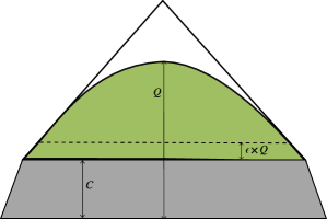
B.2 Bound on the asymptotic scenario
In the previous section we have considered the standard Bell scenario, where a single copy of a bipartite state is shared between Alice and Bob. However, if the state is distillable, as it was noted by Peres [Per96a], a pre-processing of many copies of a state by LOCC, before the Bell test, could lead to the violation of a Bell inequality, even for states that have local model in the standard scenario. Here we quantify the asymptotic nonlocality by defining the asymptotic relative entropy of nonlocality and applying methods of Ref. [BCHW15] to bound it. In the first step, we will bound this quantity by a function of the relative entropy distance under restrictive measurements introduced by Piani in Ref. [Pia09].
In Ref. [vDGG05] a nonlocality quantifier, based on the relative entropy, was introduced. The relative entropy between two probability distributions, and , is defined as . The statistical strength of nonlocality defined in Ref. [vDGG05] captures quantitatively how “similar” a given probability distribution is to a local one: Given a box , where for fixed we have distribution , its nonlocality is quantified by
| (B.13) |
where infimum in the above is taken over all local boxes, , for the particular scenario and is the relative entropy.
Now, we are interested in quantifying how much nonlocality one can obtain from copies of a given state , per number of copies, in the asymptotic limit, after processing it by LOCC. For that we introduce the asymptotic relative entropy of nonlocality.
Definition B.2.1.
For a bipartite state its asymptotic relative entropy of nonlocality, , is given by:
| (B.14) |
where is the supremum limit, and denote local POVMs .
The asymptotic relative entropy of nonlocality captures the idea of an optimization over all Bell scenarios after a pre-processing of many copies of a quantum state by LOCC operations.
We want to set bounds for the nonlocality attainable in the asymptotic scenario. In order to state the bound, we will need a well known entanglement measure called relative entropy of entanglement [VPRK97]:
| (B.15) |
where is the quantum relative entropy.
Now we are ready to state the main result of this Section.
Theorem B.2.1.
For any bipartite state it holds that
| (B.16) |
For a PPT state, it holds that
| (B.17) |
The upper bound gives meaningful results only when the state is close to separable states under global operations. More important is the second bound, which can give meaningful results even for some states which are highly distinguishable from separable states by global operations, but cannot be distinguished if only PPT operations are allowed. We refer the reader to Ref. [HM15] for the proof of Theorem B.2.1.
We can also extend Theorem B.2.1 to asymptotic scenarios where the parties can perform a ‘filtering’ operation (a non-trace-preserving map) before the Bell test: the so called hidden nonlocality scenario, introduced by Popescu in Ref. [Pop95]. Popescu showed that by performing a ‘filtering’ operation it is possible to obtain a much larger violation of a Bell inequality on the resulting state. However, we note that, in order to quantify nonlocality in this scenario, it is important to take into account the probability of obtaining the ‘filtered’ result. For this reason, we propose to consider the asymptotic relative entropy of hidden-nonlocality, , defined as follows:
| (B.18) |
Where we can see a filtering process as an operation that takes the state to a flag form
| (B.19) |
and later erasures all other results except the “good” one, that leads to the highest violation of the Bell inequality. The probability that the filter results in the desired outcome is given by
| (B.20) |
We can have the same bound for , as for .
Theorem B.2.2.
For any bipartite state it holds that
| (B.21) |
For a bipartite PPT state it holds that
| (B.22) |
B.3 Examples
In Ref. [HHHO05], it was shown that the general form of a quantum state from which it is possible to extract one bit of classical private key, a private bit, is given by
where is an arbitrary operator with trace norm 1 acting on . .
Consider a private state defined by being the (normalized) swap operator. Then for the CHSH inequality we have the following bound [Hor08]:
| (B.23) |
In [ACPA10] it was shown that all perfect private states violate the CHSH inequality. With our techniques we can bound this violation and also analyze PPT approximate private states.
Consider the following PPT approximate private state:
| (B.24) |
with and , , and . By Theorem B.1.1, we have
| (B.25) |
In Ref. [HHHO05], it was shown that there exists a family of states invariant under partial transposition for which the distillable key can be made arbitrarily close to one, . By applying Theorem B.1.1 to this family of states we obtain the following proposition.
Proposition B.3.1.
There exist bipartite states with , satisfying with increasing , such that:
| (B.26) |
Proposition B.3.1 shows that for the class of states in consideration, although the rate of distillable key can be made arbitrarily close to one by increasing the dimension of the systems, the possibility of violating any Bell inequality is bounded by an amount vanishing with the dimension of the system. For a bipartite Bell inequality with inputs and outputs it holds that , up to some universal constant independent of the parameters of the scenario [JP11]. Therefore, Theorem B.1.1 ensures that for any fixed Bell scenario, as we wish to increase the key rate obtained from the exhibited family of states, the possibility of observing a violation of a Bell inequality vanishes.
An application of Theorems B.2.1 and B.2.2 follows from the fact that the relative entropy of entanglement, , is asymptotically continuous222A function is asymptotically continuous if (B.27) where is a constant and . [SRH06]. Generally, for , and , we have:
Hence, if decreases with faster than , the asymptotic relative entropy of nonlocality vanishes with increasing dimension The family of states shown in Eq. (B.24) have this property.
B.4 Discussion and open problems
We have presented bounds on the quantum nonlocality of a bipartite state, both, in the single copy case, as well as in the asymptotic scenarios. Although we use partial transposition techniques for obtaining nontrivial results, our method is based on the concept of state discrimination via a restricted classes of operations: the separable ones.
As future directions exploring the bounds: For the single copy scenario, instead of discrimination from separable states, a refinement would be to consider the distance from states admitting a local hidden-variable model, which could possibly lead to tighter bounds; For the asymptotic scenarios, it would be interesting to find nontrivial upper bounds on the asymptotic relative entropy of (hidden) nonlocality of NPT states. Note that, for these states, we only have as an upper bound, which is small only for the cases where the state is almost indistinguishable from a separable state under global operations.
In Refs. [HHH+08, HLLO06] it was shown that one can launch quantum key distribution (QKD) protocols based on shared private bits. However, if we are interested in device-independent quantum key distribution (DI QKD) protocols we need to have a violate of some Bell inequality. A DI QKD protocol is based on some Bell inequality , and admits some level of violation, say , below which it aborts. Now, due to Eqs. (B.25) and (B.26) there are (approximate) private bits, which exhibit violation of inequality only up to , and hence will be aborted. This rules out such states from usage in this particular DI QKD protocol. Moreover, every realization of a DI QKD has inevitable errors. In such a case, the level of violation can be even below the precision of the experiment. An interesting question for further investigation is the difference in terms of key rates between QKD and DI QKD protocols.
It is worth noting, that our results are strongly related to the so called Peres conjecture [Per99], recently disproved in [VB14]. Namely, we have asked a quantitative rephrasing of the original question posed by Asher Peres: how much one can violate a Bell inequality with PPT states? We have shown that, for certain PPT states, the level of violation, both for single copy as well as in terms of the relative entropy of (hidden) nonlocality in the asymptotic cases, can be negligible. Notably, as we showed in the examples, even some states containing privacy admit such limited nonlocality content.
Appendix C A group of facts about groups
In Chapters 6 and 7 we have discussed a class of games associated to finite Abelian groups. Here we state some results and properties of finite Abelian groups. For more details the reader in referred to the book [Ter99].
C.1 Some definitions
Definition C.1 (Group).
A group is a set of elements with the associated operation satisfying
-
(i)
, ,
-
(ii)
s.t. ,
-
(iii)
s.t. ,
-
(iv)
Associativity holds:
Definition C.2 (Abelian group).
An Abelian group is a group with associated operation denoted by that, additionally to properties -, also satisfies commutativity:
| (C.1) |
Definition C.3 (Cyclic group).
A group is called cyclic if it can be generated by a single element , called the generator of the group.
A finite cyclic group is a group with the property that all the elements can be obtained by starting with the generator and applying the group operation to it many times, i.e. . This makes it clear that all finite cyclic groups are Abelian groups.
Definition C.4 (Homomorphism).
An homomorphism of a group into a group is a function such that
| (C.2) |
A remarkable example of these concepts is given by the cyclic group , for which:
-
•
.
-
•
The associated operation is the sum modulo .
-
•
The identity element is .
-
•
The inverse element of is .
-
•
is a generator111A cyclic group can have more than one generator. For example, for prime , every element of is a generator. for all .
-
•
An homomorphism from to the group of unitary complex numbers with the product operation is given by
(C.3)
C.2 The characters of an Abelian group
Definition C.5.
A character of a finite Abelian group is a group homomorphism from to the group of unitary complex numbers with the product operation:
| (C.4) |
By Definition C.5 we have that the characters of an Abelian group are complex numbers satisfying the properties:
| (C.5) |
For the cyclic group , the characters are the roots of unit
| (C.6) |
where .
A very interesting result is the called fundamental theorem of finite Abelian groups (see Ref. [Ter99]), which states that any finite Abelian group can be seen as a direct product of cyclic groups
| (C.7) |
where every element is as a -tuple with and the operation in is given by
| (C.8) |
With this characterization, the characters of the Abelian group , can be written as the product of the characters of the cyclic groups that compose :
| (C.9) |
where is a -th root of unity, and .
C.3 The Fourier transform over finite Abelian groups
A Fourier transform can be seen as a change of basis, where we pass from a description of a function in terms of a set of variables to a description in terms of different variables, but keeping all the information about . When we have a function of the elements of a finite Abelian group, the Fourier transform can be expressed in terms of the characters of the group.
Let be a complex valued function on the finite Abelian group
The Fourier transform of is defined as :
| (C.10) |
with the inverse given by
| (C.11) |
For non-Abelian groups the characters are more subtle, and the Fourier transform uses the irreducible representations of the group. For the reader interested in a further reading about Fourier transform on groups we refer to Ref. [Ter99].
C.4 Finite Fields
Fields are sets which have more structure than an Abelian group. While for an Abelian group we only have the associated sum operation , a field has two associated operations and satisfying the properties specified bellow.
Definition C.6 (Finite Field).
A finite field is a set of elements with the operations sum and multiplication such that
-
(i)
, , ,
-
(ii)
s.t. ,
-
(iii)
s.t. ,
-
(iv)
s.t. ,
-
(v)
s.t. ,
-
(vi)
Associativity:
-
(vii)
Commutativity:
-
(viii)
Distributivity:
(C.12)
Finite fields can only be defined for a set of prime or a power of prime elements. For prime all the conditions - can be satisfied by arithmetic modulo . For the arithmetic operations222See https://en.wikipedia.org/wiki/Finite_field_arithmetic. can be defined by addition and multiplication of polynomials of degree over , . In order to construct a field one can start by choosing an irreducible polynomial of degree over , this polynomial will define the zero of the field by the so called quotient.
As an example for the field with we can pick the polynomial from which we can obtain the relation
| (C.13) |
Now the elements of the field can be represented by strings , with , and we can associate each string with the polynomial . Given that, addition and multiplication will be taken as addition and multiplication of polynomials reduced by the relation (C.13).
Appendix D Functional boxes and multipartite communication complexity
Here we discuss functional boxes and the communication complexity task in the multipartite scenario. These results were also presented in Ref. [MRMT16].
We start by defining the - boxes, a generalization of boxes [PR94] for parties and prime outputs.
Definition D.1.
| (D.1) |
where is prime and sum and multiplication are operations modulo .
A multipartite communication complexity scenario consists of parties, denoted , where each party receives an input , and their goal is to exchange the least number of classical messages in order to compute the value of a global function of their inputs .
In what follows we prove that if the parties have access to a sufficient large amount of - boxes, they can compute any function with only dits of communication: where each player communicate one dit to player which them computes the function.
Theorem D.1.
If parties are allowed to share an arbitrary number of - boxes, any -partite communication complexity problem can be solved with only dits of communication.
Proof.
Our proof is a straightforward generalization of Ref. [Wan11]. We prove for the case . The proof for general follows directly.
Let us consider that Alice receives input string , Bob receives and Charlie receives . We start by observing that any function , , can be written as a multivariate polynomial with degree at most in each variable and
| (D.2) |
where , , , , and . And analogously for and . Now if the players have access to - boxes they can execute the following protocol in order to compute :
-
1.
For each the players picks one -,
-
2.
Alice inputs . Bob inputs . Charlie inputs . And they get respectively the outputs , and .
-
3.
Bob sets and send to Alice. Charlie sets and send to Alice.
-
4.
Alice sets and she computes .
where only 2 dits were communicated in order to compute the function.
The generalization for -party function follows in analogous way, where any function will be written as a multivariate polynomial with degree at most in each variable and using an analogous protocol, with parties communicating only one dit to the first party, the computation of function will be performed. ∎
Now we consider a natural generalization of bipartite functional boxes, introduced in Ref. [Wan11], to the multipartite case:
Definition D.2.
For any function , the multipartite functional box corresponding to is defined as
| (D.3) |
Now we argue that all -partite functional box with non-additively separable ( is additively separable if ) would lead to some kind of trivialization of communication complexity.
Theorem D.2.
All with such that there exists a partial derivative of some order equals to can be used to simulate a -, and then can be used to solve any -partite communication complexity problem with only dits of communication.
Proof.
First let us consider
| (D.4) |
So by using box Alice, Bob and Charlie can input and respectively and get outputs , and . Now following Ref. [Wan11] Alice sets , Bob sets and Charlie sets , so that we have
| (D.5) |
In order to randomize the results they can randomly chose and output , and , so that they perfectly simulate a - box.
Now for other functions we can use the method of Ref. [Wan11] of applying partial derivatives to the function. The partial derivative of with respect to is defined as
| (D.6) |
and it generates a polynomial with the degree in reduced by 1, while the degree in and remains the same or is smaller. And note that with two boxes we can simulate the box .
If a function is not additively separable it will contain at least one term involving product of two variables, for example and this box can be reduced, by derivatives, into a box of the form . Now using the results for the bipartite case [Wan11], if Charlie always inputs , with only 2 dits of communication they can compute any function of two variables .
Appendix E Proofs of some results
E.1 Some proofs on xor games
Theorem E.1.
Given a bipartite xor-game, with inputs for Alice, inputs for Bob, and an associated game matrix , the quantum value is upper bounded by
| (E.1) |
Proof.
We now prove this result using Lagrange duality. Let us consider the SDP characterization given by Theorem 3.2.2:
| (E.2) |
By weak duality (Theorem 2.3.1), every feasible solution to the dual Lagrange problem provides an upper bound to the quantum bias . So let us consider the dual problem of (E.2):
| (E.3) |
Note that for all is a feasible solution to problem , since and then
| (E.4) |
Therefore we have that
| (E.5) |
Now
| (E.6) |
which ends the proof. ∎
For the case where and , the same analysis results in the upper bound
| (E.7) |
which is worse then the bound given by Theorem 3.2.3.
Theorem E.1.1.
The adjacency matrix of an xor-game graph
| (E.8) | ||||
has the following spectrum and corresponding degeneracies:
| (E.9) |
where denotes the singular values of .
Proof.
We start by nothing that the adjacency matrix, Eq. (E.8), can be written in the form
| (E.10) | ||||
which allows us to write it as a direct sum
| (E.11) |
where
| (E.12) | ||||
Therefore we can proceed to diagonalize and separately.
Let us start with the eigenvalues of . Note that contains only the identity and the all 1’s matrix , therefore an eigenbasis for is formed by the Fourier vectors , where
| (E.13) |
with , where . Since we have that
-
•
is an eigenvector of with eigenvalue ,
-
•
and are eigenvectors with eigenvalue ,
-
•
are eigenvectors with eigenvalue -1.
which completes the diagonalization of .
Now let us proceed to find the eigenvalues of . First, note that, if and are the singular vectors of the game matrix , corresponding to the singular value , then, by using the relation , we can derive that
| (E.14) |
By using relation (E.14) one can verify that the following vectors
| (E.15) |
are eigenvectors of , with respective eigenvalues .
The remaining eigenvalues of are all equal to 1. This can be shown by the fact that subtracting an appropriate amount of the projector into the eigenvectors leaves us with identity, i.e. the following equality holds
| (E.16) |
This completes the proof. ∎
E.2 On DIEWs
Bellow we list the projective measurements , , that allow the players to win the generalized Mermin game discussed in Section 7.5, Eq. (7.46), with probability 1 when they share the state:
| (E.17a) | ||||
| (E.17b) | ||||
| (E.17c) | ||||
| (E.18a) | ||||
| (E.18b) | ||||
| (E.18c) | ||||
| (E.19a) | ||||
| (E.19b) | ||||
| (E.19c) | ||||
where .
References
- [AB09] S. Arora and B. Barak. Computational Complexity: A Modern Approach. Cambridge University Press, (2009).
- [ABB+10] M. L. Almeida, J.-D. Bancal, N. Brunner, A. Acín, N. Gisin, and S. Pironio. Guess Your Neighbor’s Input: A Multipartite Nonlocal Game with No Quantum Advantage. Phys. Rev. Lett., 104:230404, (2010). arXiv: 1003.3844.
- [ACPA10] R. Augusiak, D. Cavalcanti, G. Prettico, and A. Acín. Perfect Quantum Privacy Implies Nonlocality. Phys. Rev. Lett., 104:230401, (2010). arXiv: 0911.3274.
- [ACSA10] M. L. Almeida, D. Cavalcanti, V. Scarani, and A. Acín. Multipartite fully nonlocal quantum states. Phys. Rev. A, 81:052111, (2010). arXiv: 0911.3559.
- [ADR82] A. Aspect, J. Dalibard, and G. Roger. Experimental Test of Bell’s Inequalities Using Time- Varying Analyzers. Phys. Rev. Lett., 49:1804–1807, (1982).
- [ADTA15] R. Augusiak, M. Demianowicz, J. Tura, and A. Acín. Entanglement and Nonlocality are Inequivalent for Any Number of Parties. Phys. Rev. Lett., 115:030404, (2015). arXiv: 1407.3114.
- [AFLS15] A. Acín, T. Fritz, A. Leverrier, and A. B. Sainz. A Combinatorial Approach to Nonlocality and Contextuality. Communications in Mathematical Physics, 334(2):533–628, (2015). arXiv: 1212.4084.
- [Ara] M. Araújo. Understanding Bell’s theorem. More Quantum, Mateus Araújo’s Blog. http://mateusaraujo.info/2016/07/15/understanding-bells-theorem-part-1-the-simple-version/.
- [ATC14] B. Amaral, M. Terra Cunha, and A. Cabello. Exclusivity principle forbids sets of correlations larger than the quantum set. Phys. Rev. A, 89:030101, (2014). arXiv: 1306.6289.
- [Bar02] J. Barrett. Nonsequential positive-operator-valued measurements on entangled mixed states do not always violate a Bell inequality. Phys. Rev. A, 65:042302, (2002). arXiv: quant-ph/0107045.
- [BBB+12] J.-D. Bancal, C. Branciard, N. Brunner, N. Gisin, and Y.-C. Liang. A framework for the study of symmetric full-correlation Bell-like inequalities. Journal of Physics A: Mathematical and Theoretical, 45(12):125301, (2012). arXiv: 1201.2055.
- [BBGL11] J.-D. Bancal, N. Brunner, N. Gisin, and Y.-C. Liang. Detecting Genuine Multipartite Quantum Nonlocality: A Simple Approach and Generalization to Arbitrary Dimensions. Phys. Rev. Lett., 106:020405, (2011). arXiv: 1011.0089.
- [BBGP13] J.-D. Bancal, J. Barrett, N. Gisin, and S. Pironio. Definitions of multipartite nonlocality. Phys. Rev. A, 88:014102, (2013). arXiv: 1112.2626.
- [BBL+06] G. Brassard, H. Buhrman, N. Linden, A. A. Méthot, A. Tapp, and F. Unger. Limit on Nonlocality in Any World in Which Communication Complexity Is Not Trivial. Phys. Rev. Lett., 96:250401, (2006). arXiv: quant-ph/0508042.
- [BCHW15] S. Bauml, M. Christandl, K. Horodecki, and A. Winter. Limitations on quantum key repeaters. Nat Commun, 6, (2015). arXiv: 1402.5927.
- [BCMdW10] H. Buhrman, R. Cleve, S. Massar, and R. de Wolf. Nonlocality and communication complexity. Rev. Mod. Phys., 82:665–698, (2010). arXiv: 0907.3584.
- [BCP+14] N. Brunner, D. Cavalcanti, S. Pironio, V. Scarani, and S. Wehner. Bell nonlocality. Rev. Mod. Phys., 86:419–478, (2014). arXiv: 1303.2849.
- [BDF+99] C. H. Bennett, D. P. DiVincenzo, C. A. Fuchs, T. Mor, E. Rains, P. W. Shor, J. A. Smolin, and W. K. Wootters. Quantum nonlocality without entanglement. Phys. Rev. A, 59:1070–1091, (1999). arXiv: quant-ph/9804053.
- [Bel64] J. S. Bell. On the Eintein Podolsky Rosen paradox. Physics 1, 195-200, (1964).
- [BFF+16] J. Bowles, J. Francfort, M. Fillettaz, F. Hirsch, and N. Brunner. Genuinely Multipartite Entangled Quantum States with Fully Local Hidden Variable Models and Hidden Multipartite Nonlocality. Phys. Rev. Lett., 116:130401, (2016). arXiv: 1511.08401.
- [BGLP11] J.-D. Bancal, N. Gisin, Y.-C. Liang, and S. Pironio. Device-Independent Witnesses of Genuine Multipartite Entanglement. Phys. Rev. Lett., 106:250404, (2011). arXiv: 1102.0197.
- [BM05] H. Buhrman and S. Massar. Causality and Tsirelson’s bounds. Phys. Rev. A, 72:052103, (2005). arXiv: quant-ph/0409066.
- [BOGKW88] M. Ben-Or, S. Goldwasser, J. Kilian, and A. Wigderson. Multi-prover Interactive Proofs: How to Remove Intractability Assumptions. In Proceedings of the Twentieth Annual ACM Symposium on Theory of Computing, STOC ’88, pages 113–131, New York, NY, USA, (1988). ACM.
- [Bor26] M. Born. Zur Quantenmechanik der Stossvorgänge. (English translation: On the quantum mechanics of collisions, in Quantum theory and measurement, section I.2, J. A. Wheeler and W. H. Zurek, Princeton University Press, 1983). Zeitschrift für Physik, 37(12):863–867, (1926).
- [BP05] J. Barrett and S. Pironio. Popescu-Rohrlich Correlations as a Unit of Nonlocality. Phys. Rev. Lett., 95:140401, (2005). arXiv: quant-ph/0506180.
- [BPT00] H. Bechmann-Pasquinucci and W. Tittel. Quantum cryptography using larger alphabets. Phys. Rev. A, 61:062308, (2000). arXiv: quant-ph/9910095.
- [BS15] M. Bavarian and P. W. Shor. Information Causality, Szemerédi-Trotter and Algebraic Variants of CHSH. In Proceedings of the 2015 Conference on Innovations in Theoretical Computer Science, ITCS ’15, pages 123–132, New York, NY, USA, (2015). ACM. arXiv: 1311.5186.
- [BTN13] A. Ben-Tal and A. Nemirovski. Lectures on Modern Convex Optimization. (2013). Online version: http://www2.isye.gatech.edu/~nemirovs/Lect_ModConvOpt.
- [BV04] S. Boyd and L. Vandenberghe. Convex Optimization. Cambridge University Press, (2004).
- [BV12] N. Brunner and T. Vértesi. Persistency of entanglement and nonlocality in multipartite quantum systems. Phys. Rev. A, 86:042113, (2012). arXiv: 1207.3986.
- [BZPZ04] Č. Brukner, M. Żukowski, J.-W. Pan, and A. Zeilinger. Bell’s Inequalities and Quantum Communication Complexity. Phys. Rev. Lett., 92:127901, (2004). arXiv: quant-ph/0210114.
- [CABV13] D. Cavalcanti, A. Acín, N. Brunner, and T. Vértesi. All quantum states useful for teleportation are nonlocal resources. Phys. Rev. A, 87:042104, (2013). arXiv: 1207.5485.
- [CASA11] D. Cavalcanti, M. L. Almeida, V. Scarani, and A. Acin. Quantum networks reveal quantum nonlocality. Nat Commun, 2:184, (2011). arXiv: 1010.0900.
- [CDLTP13] A. Cabello, L. E. Danielsen, A. J. López-Tarrida, and J. R. Portillo. Basic exclusivity graphs in quantum correlations. Phys. Rev. A, 88:032104, (2013). arXiv: 1211.5825.
- [CGP+02] D. Collins, N. Gisin, S. Popescu, D. Roberts, and V. Scarani. Bell-Type Inequalities to Detect True -Body Nonseparability. Phys. Rev. Lett., 88:170405, (2002). arXiv: quant-ph/0201058.
- [CGRS16] D. Cavalcanti, L. Guerini, R. Rabelo, and P. Skrzypczyk. General Method for Constructing Local Hidden Variable Models for Entangled Quantum States. Phys. Rev. Lett., 117:190401, (2016). arXiv: 1512.00277.
- [CH74] J. F. Clauser and M. A. Horne. Experimental consequences of objective local theories. Phys. Rev. D, 10:526–535, (1974).
- [CHSH69] J. F. Clauser, M. A. Horne, A. Shimony, and R. A. Holt. Proposed Experiment to Test Local Hidden-Variable Theories. Phys. Rev. Lett., 23:880–884, (1969).
- [CHTW04] R. Cleve, P. Hoyer, B. Toner, and J. Watrous. Consequences and limits of nonlocal strategies. In Computational Complexity, 2004. Proceedings. 19th IEEE Annual Conference on, pages 236–249, (2004). arXiv: quant-ph/0404076.
- [Cir80] B. Cirel’son. Quantum generalizations of Bell’s inequality. Letters in Mathematical Physics, 4(2):93–100, (1980).
- [CMSS14] A. Chailloux, L. Mancinska, G. Scarpa, and S. Severini. Graph-theoretical Bounds on the Entangled Value of Non-local Games. In 9th Conference on the Theory of Quantum Computation, Communication and Cryptography (TQC 2014), volume 27 of Leibniz International Proceedings in Informatics (LIPIcs), pages 67–75, (2014). arXiv: 1404.3640.
- [Cob65] A. Cobham. The intrinsic computational difficulty of functions. In B.-H. Yehoshua, editor, Proceedings of the 1964 International Congress, Studies in logic and the foundations of mathematicss, pages 24–30. North-Holland Publishing Company, (1965).
- [Coo71] S. A. Cook. The Complexity of Theorem-proving Procedures. In Proceedings of the Third Annual ACM Symposium on Theory of Computing, STOC ’71, pages 151–158, New York, NY, USA, (1971). ACM.
- [CR12] R. Colbeck and R. Renner. Free randomness can be amplified. Nat Phys, 8(6):450–453, (2012). arXiv: 1105.3195.
- [CRS12] D. Cavalcanti, R. Rabelo, and V. Scarani. Nonlocality Tests Enhanced by a Third Observer. Phys. Rev. Lett., 108:040402, (2012). arXiv: 1110.3656.
- [CSUU08] R. Cleve, W. Slofstra, F. Unger, and S. Upadhyay. Perfect Parallel Repetition Theorem for Quantum Xor Proof Systems. computational complexity, 17(2):282–299, (2008). arXiv: quant-ph/0608146.
- [CSW10] A. Cabello, S. Severini, and A. Winter. (Non-)Contextuality of Physical Theories as an Axiom. (2010). arXiv: 1010.2163.
- [CSW14] A. Cabello, S. Severini, and A. Winter. Graph-Theoretic Approach to Quantum Correlations. Phys. Rev. Lett., 112:040401, (2014). arXiv: 1401.7081.
- [Die10] R. Diestel. Graph Theory, volume 173 of Graduate Texts in Mathematics. Springer-Verlag New York, 4th edition, (2010). Electronic Edition: http://diestel-graph-theory.com/index.html.
- [Dir39] P. A. M. Dirac. A new notation for quantum mechanics. Mathematical Proceedings of the Cambridge Philosophical Society, 35:416–418, (1939).
- [DLT02] D. P. DiVincenzo, D. Leung, and B. Terhal. Quantum data hiding. Information Theory, IEEE Transactions on, 48(3):580–598, (2002). arXiv: quant-ph/0103098.
- [DO12] R. C. Drumond and R. I. Oliveira. Small violations of full-correlation Bell inequalities for multipartite pure random states. Phys. Rev. A, 86:012117, (2012). arXiv: 1209.1755.
- [DVC00] W. Dür, G. Vidal, and J. I. Cirac. Three qubits can be entangled in two inequivalent ways. Phys. Rev. A, 62:062314, (2000). arXiv: quant-ph/0005115.
- [Ebe93] P. H. Eberhard. Background level and counter efficiencies required for a loophole-free Einstein-Podolsky-Rosen experiment. Phys. Rev. A, 47:R747–R750, (1993).
- [ECG+13] S. Etcheverry, G. Cañas, E. S. Gómez, W. A. T. Nogueira, C. Saavedra, G. B. Xavier, and G. Lima. Quantum key distribution session with 16-dimensional photonic states. Scientific Reports, 3:2316, (2013). arXiv: 1308.0019.
- [Edm87] J. Edmonds. Paths, Trees, and Flowers. In I. Gessel and G.-C. Rota, editors, Classic Papers in Combinatorics, Modern Birkhäuser Classics, pages 361–379. Birkhäuser Boston, (1987).
- [EKB13] M. Epping, H. Kampermann, and D. Bruß. Designing Bell Inequalities from a Tsirelson Bound. Phys. Rev. Lett., 111:240404, (2013). arXiv: 1306.3805.
- [Eke91] A. K. Ekert. Quantum cryptography based on Bell’s theorem. Phys. Rev. Lett., 67:661–663, (1991).
- [EPR35] A. Einstein, B. Podolsky, and N. Rosen. Can Quantum-Mechanical Description of Physical Reality Be Considered Complete? Phys. Rev., 47:777–780, (1935).
- [EW02] T. Eggeling and R. F. Werner. Hiding Classical Data in Multipartite Quantum States. Phys. Rev. Lett., 89:097905, (2002). arXiv: quant-ph/0203004.
- [Fey65] R. P. Feynman. The character of physical law. The M.I.T Press, (1965). The lectures can be watched at: www.cornell.edu/video/playlist/richard-feynman-messenger-lectures.
- [Fin82] A. Fine. Hidden Variables, Joint Probability, and the Bell Inequalities. Phys. Rev. Lett., 48:291–295, (1982).
- [FSA+13] T. Fritz, A. Sainz, R. Augusiak, J. B. Brask, R. Chaves, A. Leverrier, and A. Acin. Local orthogonality as a multipartite principle for quantum correlations. Nat Commun, 4, (2013). arXiv: 1210.3018.
- [GHH10] A. Gabriel, B. C. Hiesmayr, and M. Huber. Criterion for K-separability in Mixed Multipartite States. Quantum Info. Comput., 10(9):829–836, (2010). arXiv: 1002.2953.
- [GJ90] M. R. Garey and D. S. Johnson. Computers and Intractability; A Guide to the Theory of NP-Completeness. W. H. Freeman & Co., New York, NY, USA, (1990).
- [GJV+06] S. Gröblacher, T. Jennewein, A. Vaziri, G. Weihs, and A. Zeilinger. Experimental quantum cryptography with qutrits. New Journal of Physics, 8(5):75, (2006). arXiv: quant-ph/0511163.
- [GVL96] G. H. Golub and C. F. Van Loan. Matrix Computations (3rd Ed.). Johns Hopkins University Press, Baltimore, MD, USA, (1996).
- [GVW+15] M. Giustina, M. A. M. Versteegh, S. Wengerowsky, J. Handsteiner, A. Hochrainer, K. Phelan, F. Steinlechner, J. Kofler, J.-A. Larsson, C. Abellán, W. Amaya, V. Pruneri, M. W. Mitchell, J. Beyer, T. Gerrits, A. E. Lita, L. K. Shalm, S. W. Nam, T. Scheidl, R. Ursin, B. Wittmann, and A. Zeilinger. Significant-Loophole-Free Test of Bell’s Theorem with Entangled Photons. Phys. Rev. Lett., 115:250401, (2015). arXiv: 1511.03190.
- [GWAN11] R. Gallego, L. E. Würflinger, A. Acín, and M. Navascués. Quantum Correlations Require Multipartite Information Principles. Phys. Rev. Lett., 107:210403, (2011). arXiv: 1107.3738.
- [Hås01] J. Håstad. Some Optimal Inapproximability Results. J. ACM, 48(4):798–859, (2001).
- [HBD+15] B. Hensen, H. Bernien, A. E. Dreau, A. Reiserer, N. Kalb, M. S. Blok, J. Ruitenberg, R. F. L. Vermeulen, R. N. Schouten, C. Abellan, W. Amaya, V. Pruneri, M. W. Mitchell, M. Markham, D. J. Twitchen, D. Elkouss, S. Wehner, T. H. Taminiau, and R. Hanson. Loophole-free Bell inequality violation using electron spins separated by 1.3 kilometres. Nature, 526(7575):682–686, (2015). arXiv: 1508.05949.
- [HdV13] M. Huber and J. I. de Vicente. Structure of Multidimensional Entanglement in Multipartite Systems. Phys. Rev. Lett., 110:030501, (2013). arXiv: 1210.6876.
- [HGBL05] P. Hyllus, O. Gühne, D. Bruß, and M. Lewenstein. Relations between entanglement witnesses and Bell inequalities. Phys. Rev. A, 72:012321, (2005). arXiv: quant-ph/0504079.
- [HHH96] M. Horodecki, P. Horodecki, and R. Horodecki. Separability of mixed states: necessary and sufficient conditions. Physics Letters A, 223(1–2):1 – 8, (1996). arXiv: quant-ph/9605038.
- [HHH98] M. Horodecki, P. Horodecki, and R. Horodecki. Mixed-State Entanglement and Distillation: Is there a “Bound” Entanglement in Nature? Phys. Rev. Lett., 80:5239–5242, (1998). arXiv: quant-ph/9801069.
- [HHH+08] K. Horodecki, M. Horodecki, P. Horodecki, D. Leung, and J. Oppenheim. Quantum Key Distribution Based on Private States: Unconditional Security Over Untrusted Channels With Zero Quantum Capacity. Information Theory, IEEE Transactions on, 54(6):2604–2620, (2008). arXiv: quant-ph/0608195.
- [HHHO05] K. Horodecki, M. Horodecki, P. Horodecki, and J. Oppenheim. Secure Key from Bound Entanglement. Phys. Rev. Lett., 94:160502, (2005). arXiv: quant-ph/0309110.
- [HJ12] R. A. Horn and C. R. Johnson. Matrix Analysis. Cambridge University Press, New York, NY, USA, 2nd edition, (2012).
- [HLLO06] K. Horodecki, D. Leung, H.-K. Lo, and J. Oppenheim. Quantum Key Distribution Based on Arbitrarily Weak Distillable Entangled States. Phys. Rev. Lett., 96:070501, (2006). arXiv: quant-ph/0510067.
- [HM15] K. Horodecki and G. Murta. Bounds on quantum nonlocality via partial transposition. Phys. Rev. A, 92:010301, (2015). arXiv: 1407.6999.
- [Hor08] K. Horodecki. General paradigm for distilling classical key from quantum states — On quantum entanglement and security. PhD thesis, University of Warsaw, (2008).
- [HP13] M. Huber and M. Pawłowski. Weak randomness in device-independent quantum key distribution and the advantage of using high-dimensional entanglement. Phys. Rev. A, 88:032309, (2013). arXiv: 1301.2455.
- [HQBB13] F. Hirsch, M. T. Quintino, J. Bowles, and N. Brunner. Genuine Hidden Quantum Nonlocality. Phys. Rev. Lett., 111:160402, (2013). arXiv: 1307.4404.
- [HQV+16] F. Hirsch, M. T. Quintino, T. Vértesi, M. F. Pusey, and N. Brunner. Algorithmic Construction of Local Hidden Variable Models for Entangled Quantum States. Phys. Rev. Lett., 117:190402, (2016). arXiv: 1512.00262.
- [HS14] M. Huber and R. Sengupta. Witnessing Genuine Multipartite Entanglement with Positive Maps. Phys. Rev. Lett., 113:100501, (2014). arXiv: 1404.7449.
- [JLL+08] S.-W. Ji, J. Lee, J. Lim, K. Nagata, and H.-W. Lee. Multisetting Bell inequality for qudits. Phys. Rev. A, 78:052103, (2008). arXiv: 0810.2838.
- [JNP+11] M. Junge, M. Navascues, C. Palazuelos, D. Perez-Garcia, V. B. Scholz, and R. F. Werner. Connes’ embedding problem and Tsirelson’s problem. Journal of Mathematical Physics, 52(1), (2011). arXiv: 1008.1142.
- [JP11] M. Junge and C. Palazuelos. Large Violation of Bell Inequalities with Low Entanglement. Communications in Mathematical Physics, 306(3):695–746, (2011). arXiv: 1007.3043.
- [Kar72] R. Karp. Reducibility among Combinatorial Problems. In R. Miller, J. Thatcher, and J. Bohlinger, editors, Complexity of Computer Computations, The IBM Research Symposia Series, pages 85–103. Springer US, (1972).
- [Kav] Kaveh(http://cs.stackexchange.com/users/41/kaveh). What is the definition of P, NP, NP-complete and NP-hard? Computer Science Stack Exchange. http://cs.stackexchange.com/q/18666 (version: 2013-12-06).
- [KC16] M. Kleinmann and A. Cabello. Quantum Correlations Are Stronger Than All Nonsignaling Correlations Produced by -Outcome Measurements. Phys. Rev. Lett., 117:150401, (2016). arXiv: 1505.04179.
- [Ken11] A. Kent. Unconditionally secure bit commitment with flying qudits. New Journal of Physics, 13(11):113015, (2011). arXiv: 1101.4620.
- [Ken12] A. Kent. Unconditionally Secure Bit Commitment by Transmitting Measurement Outcomes. Phys. Rev. Lett., 109:130501, (2012). arXiv: 1108.2879.
- [KKMO07] S. Khot, G. Kindler, E. Mossel, and R. O’Donnell. Optimal Inapproximability Results for MAX-CUT and Other 2-Variable CSPs? SIAM J. Comput., 37(1):319–357, (2007).
- [Knu94] D. E. Knuth. The Sandwich Theorem. The Electronic Journal of Combinatorics, 1:# A1, (1994). arXiv: math/9312214.
- [KRT10] J. Kempe, O. Regev, and B. Toner. Unique Games with Entangled Provers Are Easy. SIAM J. Comput., 39(7):3207–3229, (2010). arXiv: 0710.0655.
- [KT85] L. Khalfin and B. Tsirelson. Quantum and quasi-classical analogs of Bell inequalities. Symposium on the Foundations of Modern Physics 1985, pages 441–460, (1985).
- [KTHW13] J. Kaniewski, M. Tomamichel, E. Hanggi, and S. Wehner. Secure Bit Commitment From Relativistic Constraints. Information Theory, IEEE Transactions on, 59(7):4687–4699, (2013). arXiv: 1206.1740.
- [Lar13] C. E. Larson. A Class of Graphs Where Alpha=Theta. The Conjecturing Project, (2013). https://independencenumber.wordpress.com/2013/12/09/a-class-of-graphs-where-alphatheta/.
- [LC97] H.-K. Lo and H. F. Chau. Is Quantum Bit Commitment Really Possible? Phys. Rev. Lett., 78:3410–3413, (1997). arXiv: quant-ph/9603004.
- [Lev73] L. Levin. Universal search problems (Russian: Universal’nye perebornye zadachi). Problems of Information Transmission (Russian: Problemy Peredachi Informatsii), 9(3):265–266, (1973). Translated into English by Trakhtenbrot, B. A. (1984). "A Survey of Russian Approaches to Perebor (Brute-Force Searches) Algorithms". Annals of the History of Computing 6 (4): 384–400.
- [LLD09] Y.-C. Liang, C.-W. Lim, and D.-L. Deng. Reexamination of a multisetting Bell inequality for qudits. Phys. Rev. A, 80:052116, (2009). arXiv: 0903.4964.
- [Lov79] L. Lovasz. On the Shannon capacity of a graph. Information Theory, IEEE Transactions on, 25(1):1–7, (1979).
- [Lov09] L. Lovász. Geometric representations of graphs. (2009). Lecture notes: www.cs.elte.hu/~lovasz/geomrep.pdf.
- [LPSW07] N. Linden, S. Popescu, A. J. Short, and A. Winter. Quantum Nonlocality and Beyond: Limits from Nonlocal Computation. Phys. Rev. Lett., 99:180502, (2007). arXiv: quant-ph/0610097.
- [Mas03] L. Masanes. Necessary and sufficient condition for quantum-generated correlations. (2003). arXiv: quant-ph/0309137.
- [May97] D. Mayers. Unconditionally Secure Quantum Bit Commitment is Impossible. Phys. Rev. Lett., 78:3414–3417, (1997). arXiv: quant-ph/9605044.
- [MBL+13] T. Moroder, J.-D. Bancal, Y.-C. Liang, M. Hofmann, and O. Gühne. Device-Independent Entanglement Quantification and Related Applications. Phys. Rev. Lett., 111:030501, (2013). arXiv: 1302.1336.
- [MCC+11] Z.-H. Ma, Z.-H. Chen, J.-L. Chen, C. Spengler, A. Gabriel, and M. Huber. Measure of genuine multipartite entanglement with computable lower bounds. Phys. Rev. A, 83:062325, (2011). arXiv: 1101.2001.
- [Mer90] N. D. Mermin. Extreme quantum entanglement in a superposition of macroscopically distinct states. Phys. Rev. Lett., 65:1838–1840, (1990).
- [MPA11] L. Masanes, S. Pironio, and A. Acin. Secure device-independent quantum key distribution with causally independent measurement devices. Nat Commun, 2:238, (2011). arXiv: 1009.1567.
- [MRMT16] G. Murta, R. Ramanathan, N. Móller, and M. Terra Cunha. Quantum bounds on multiplayer linear games and device-independent witness of genuine tripartite entanglement. Phys. Rev. A, 93:022305, (2016). arXiv: 1510.09210.
- [Mur12] G. Murta. Não-Localidade em Sistemas Quânticos. Master thesis. Programa de Pós-Graduação em Física - UFMG, (2012).
- [MVWZ01] A. Mair, A. Vaziri, G. Weihs, and A. Zeilinger. Entanglement of the orbital angular momentum states of photons. Nature, 412:313–316, (2001). arXiv: quant-ph/0104070.
- [NC10] M. A. Nielsen and I. L. Chuang. Quantum Computation and Quantum Information. Cambridge University Press, (2010).
- [NCPGV12] M. Navascués, T. Cooney, D. Pérez-García, and N. Villanueva. A Physical Approach to Tsirelson’s Problem. Foundations of Physics, 42(8):985–995, (2012). arXiv: 1105.3373.
- [NPA08] M. Navascués, S. Pironio, and A. Acín. A convergent hierarchy of semidefinite programs characterizing the set of quantum correlations. New Journal of Physics, 10(7):073013, (2008). arXiv: 0803.4290.
- [PAB+09] S. Pironio, A. Acín, N. Brunner, N. Gisin, S. Massar, and V. Scarani. Device-independent quantum key distribution secure against collective attacks. New Journal of Physics, 11(4):045021, (2009). arXiv: 0903.4460.
- [Pal12] C. Palazuelos. Superactivation of Quantum Nonlocality. Phys. Rev. Lett., 109:190401, (2012). arXiv: 1205.3118.
- [PAM+10] S. Pironio, A. Acín, S. Massar, A. B. de la Giroday, D. N. Matsukevich, P. Maunz, S. Olmschenk, D. Hayes, L. Luo, T. A. Manning, and C. Monroe. Random numbers certified by Bell’s theorem. Nature, 464(7291):1021–1024, (2010). arXiv: 0911.3427.
- [Pen89] R. Penrose. The Emperor’s New Mind: Concerning Computers, Minds, and the Laws of Physics. Oxford University Press, Inc., New York, NY, USA, (1989).
- [Per96a] A. Peres. Collective tests for quantum nonlocality. Phys. Rev. A, 54:2685–2689, (1996). arXiv: quant-ph/9603023.
- [Per96b] A. Peres. Separability Criterion for Density Matrices. Phys. Rev. Lett., 77:1413–1415, (1996). arXiv: quant-ph/9604005.
- [Per99] A. Peres. All the Bell Inequalities. Foundations of Physics, 29(4):589–614, (1999). arXiv: quant-ph/9807017.
- [Pia09] M. Piani. Relative Entropy of Entanglement and Restricted Measurements. Phys. Rev. Lett., 103:160504, (2009). arXiv: 0904.2705.
- [Pir04] S. Pironio. Aspects of Quantum Non Locality. PhD thesis, Université Libre de Bruxelles, (2004).
- [Pop95] S. Popescu. Bell’s Inequalities and Density Matrices: Revealing “Hidden” Nonlocality. Phys. Rev. Lett., 74:2619–2622, (1995). arXiv: quant-ph/9502005.
- [PPK+09] M. Pawlowski, T. Paterek, D. Kaszlikowski, V. Scarani, A. Winter, and M. Żukowski. Information causality as a physical principle. Nature, 461(7267):1101–1104, (2009). arXiv: 0905.2292.
- [PR94] S. Popescu and D. Rohrlich. Quantum nonlocality as an axiom. Foundations of Physics, 24(3):379–385, (1994). arXiv: quant-ph/9508009.
- [PV11] K. F. Pál and T. Vértesi. Multisetting Bell-type inequalities for detecting genuine multipartite entanglement. Phys. Rev. A, 83:062123, (2011). arXiv: 1102.4320.
- [QBHB16] M. T. Quintino, J. Bowles, F. Hirsch, and N. Brunner. Incompatible quantum measurements admitting a local-hidden-variable model. Phys. Rev. A, 93:052115, (2016). arXiv: 1510.06722.
- [Qui12] M. T. Quintino. Black Box Correlations: Locality, Noncontextuality, and Convex Polytopes. Master thesis. Programa de Pós-Graduação em Física - UFMG, (2012).
- [Rai01] E. Rains. A semidefinite program for distillable entanglement. Information Theory, IEEE Transactions on, 47(7):2921–2933, (2001). arXiv: quant-ph/0008047.
- [RAM16] R. Ramanathan, R. Augusiak, and G. Murta. Generalized xor games with outcomes and the task of nonlocal computation. Phys. Rev. A, 93:022333, (2016). arXiv: 1502.02974.
- [RDLT+14] R. Rabelo, C. Duarte, A. J. López-Tarrida, M. Terra Cunha, and A. Cabello. Multigraph approach to quantum non-locality. Journal of Physics A: Mathematical and Theoretical, 47(42):424021, (2014). arXiv: 1407.5340.
- [RKMH14] R. Ramanathan, A. Kay, G. Murta, and P. Horodecki. Characterizing the Performance of xor Games and the Shannon Capacity of Graphs. Phys. Rev. Lett., 113:240401, (2014). arXiv: 1406.0995.
- [RQS+17] R. Ramanathan, M. T. Quintino, A. B. Sainz, G. Murta, and R. Augusiak. Tightness of correlation inequalities with no quantum violation. Phys. Rev. A, 95:012139, (2017). arXiv: 1607.05714.
- [RTHH16] R. Ramanathan, J. Tuziemski, M. Horodecki, and P. Horodecki. No Quantum Realization of Extremal No-Signaling Boxes. Phys. Rev. Lett., 117:050401, (2016). arXiv: 1410.0947.
- [Sha48] C. Shannon. A mathematical theory of communication. Bell System Technical Journal, The, 27(3):379–423, (1948).
- [Sha56] C. Shannon. The zero error capacity of a noisy channel. Information Theory, IRE Transactions on, 2(3):8–19, (1956).
- [SMSC+15] L. K. Shalm, E. Meyer-Scott, B. G. Christensen, P. Bierhorst, M. A. Wayne, M. J. Stevens, T. Gerrits, S. Glancy, D. R. Hamel, M. S. Allman, K. J. Coakley, S. D. Dyer, C. Hodge, A. E. Lita, V. B. Verma, C. Lambrocco, E. Tortorici, A. L. Migdall, Y. Zhang, D. R. Kumor, W. H. Farr, F. Marsili, M. D. Shaw, J. A. Stern, C. Abellán, W. Amaya, V. Pruneri, T. Jennewein, M. W. Mitchell, P. G. Kwiat, J. C. Bienfang, R. P. Mirin, E. Knill, and S. W. Nam. Strong Loophole-Free Test of Local Realism*. Phys. Rev. Lett., 115:250402, (2015). arXiv: 1511.03189.
- [SRH06] B. Synak-Radtke and M. Horodecki. On asymptotic continuity of functions of quantum states. Journal of Physics A: Mathematical and General, 39(26):L423, (2006). arXiv: quant-ph/0507126.
- [SS02] M. Seevinck and G. Svetlichny. Bell-Type Inequalities for Partial Separability in -Particle Systems and Quantum Mechanical Violations. Phys. Rev. Lett., 89:060401, (2002). arXiv: quant-ph/0201046.
- [Sve87] G. Svetlichny. Distinguishing three-body from two-body nonseparability by a Bell-type inequality. Phys. Rev. D, 35:3066–3069, (1987).
- [TDL01] B. M. Terhal, D. P. DiVincenzo, and D. W. Leung. Hiding Bits in Bell States. Phys. Rev. Lett., 86:5807–5810, (2001). arXiv: quant-ph/0011042.
- [Ter99] A. Terras. Fourier Analysis on Finite Groups and Applications. Cambridge University Press, (1999). Cambridge Books Online.
- [Ter00] B. M. Terhal. Bell inequalities and the separability criterion. Physics Letters A, 271(5–6):319 – 326, (2000). arXiv: quant-ph/9911057.
- [Tsi80] B. Tsirelson. Quantum generalizations of Bell’s inequality. Letters in Mathematical Physics, 4(2):93–100, (1980).
- [Tsi87] B. Tsirelson. Quantum analogues of the Bell inequalities. The case of two spatially separated domains. Journal of Soviet Mathematics, 36(4):557–570, (1987).
- [Tur37] A. M. Turing. On Computable Numbers, with an Application to the Entscheidungsproblem. Proceedings of the London Mathematical Society, s2-42(1):230–265, (1937).
- [VB14] T. Vértesi and N. Brunner. Disproving the Peres conjecture by showing Bell nonlocality from bound entanglement. Nat Commun, 5, (2014). arXiv: 1405.4502.
- [vD13] W. van Dam. Implausible consequences of superstrong nonlocality. Natural Computing, 12(1):9–12, (2013). arXiv: quant-ph/0501159.
- [vDGG05] W. van Dam, R. Gill, and P. Grunwald. The statistical strength of nonlocality proofs. Information Theory, IEEE Transactions on, 51(8):2812–2835, (2005). arXiv: quant-ph/0307125.
- [Vid13] T. Vidick. Three-Player Entangled XOR Games Are NP-Hard to Approximate. In Foundations of Computer Science (FOCS), 2013 IEEE 54th Annual Symposium on, pages 766–775, (2013). arXiv: 1302.1242.
- [VPRK97] V. Vedral, M. B. Plenio, M. A. Rippin, and P. L. Knight. Quantifying Entanglement. Phys. Rev. Lett., 78:2275–2279, (1997). arXiv: quant-ph/9702027.
- [VV14] U. Vazirani and T. Vidick. Fully Device-Independent Quantum Key Distribution. Phys. Rev. Lett., 113:140501, (2014). arXiv: 1210.1810.
- [Wan11] G. Wang. Functional boxes, communication complexity and information causality. (2011). arXiv: 1109.4988.
- [Weh06] S. Wehner. Tsirelson bounds for generalized Clauser-Horne-Shimony-Holt inequalities. Phys. Rev. A, 73:022110, (2006). arXiv: quant-ph/0510076.
- [Wer89] R. F. Werner. Quantum states with Einstein-Podolsky-Rosen correlations admitting a hidden-variable model. Phys. Rev. A, 40:4277–4281, (1989).
- [WLAR06] S. P. Walborn, D. S. Lemelle, M. P. Almeida, and P. H. S. Ribeiro. Quantum Key Distribution with Higher-Order Alphabets Using Spatially Encoded Qudits. Phys. Rev. Lett., 96:090501, (2006). arXiv: quant-ph/0510088.
- [WPGF09] M. M. Wolf, D. Perez-Garcia, and C. Fernandez. Measurements Incompatible in Quantum Theory Cannot Be Measured Jointly in Any Other No-Signaling Theory. Phys. Rev. Lett., 103:230402, (2009). arXiv: 0905.2998.
- [WW01a] R. F. Werner and M. M. Wolf. All-multipartite Bell-correlation inequalities for two dichotomic observables per site. Phys. Rev. A, 64:032112, (2001). arXiv: quant-ph/0102024.
- [WW01b] R. F. Werner and M. M. Wolf. Bell Inequalities and Entanglement. Quantum Info. Comput., 1(3):1–25, (2001). arXiv: quant-ph/0107093.
- [YDY14] N. Yu, R. Duan, and M. Ying. Distinguishability of Quantum States by Positive Operator-Valued Measures With Positive Partial Transpose. Information Theory, IEEE Transactions on, 60(4):2069–2079, (2014). arXiv: 1209.4222.
- [ZHHH98] M. Żukowski, R. Horodecki, M. Horodecki, and P. Horodecki. Generalized quantum measurements and local realism. Phys. Rev. A, 58:1694–1698, (1998). arXiv: quant-ph/9608035.
- [Zie95] G. M. Ziegler. Lectures on Polytopes, volume 152 of Graduate Texts in Mathematics. Springer-Verlag New York, (1995).