Abstract

In this paper, we review the discrete Hamilton–Jacobi theory from a geometric point of view. In the discrete realm, the usual geometric interpretation of the Hamilton–Jacobi theory in terms of vector fields is not straightforward.

Here, we propose two alternative interpretations: one is the interpretation in terms of projective flows, the second is the temptative of constructing a discrete Hamiltonian vector field renacting the usual continous interpretation.

Both interpretations are proven to be equivalent and applied in optimal control theory. The solutions achieved through both approaches are sorted out and compared by numerical computation.

1 Introduction

The discretization of differential equations is efficient on frameworks in which we cannot compute analytical solutions of the equation and numerical methods worked upon discretizations provide approximate solutions of our differential problem.

In recent years, there has been a growing effort to set proper discrete analogues of continuous models and design numerical methods to solve them. In this paper, we are interested in dynamical systems and optimal control problems endowed with a discrete Hamiltonian system. Hence, numerical methods in geometric mechanics must preserve symplecticity since we work on a phase space, among some other restrictions.

The first inklings of discrete mechanics appeared in the realm of Lagrangian mechanics [22]. The lack of a corresponding Hamiltonian theory lead to the development of discrete Hamiltonian mechanics. Since then, some works appeared on the discretization of Lagrangian and Hamiltonian systems on tangent and cotangent bundles, what lead to variational principles for dynamical systems and principles of critical action on both the tangent and cotangent bundle [13, 21]. This gave rise to analogies between discrete and continuous symplectic forms, Legendre transformations, momentum maps and Noether’s theorem. The Hamiltonian side specially gave rise to optimal control problems by developing a discrete maximum principle that yields discrete necessary conditions for optimality. Furthermore, discrete Hamiltonian theories have been particulary useful in distributed network optimization and derivation of variational integrators [17]. These constructions rely on numerical methods that do not only preserve symplecticity but also the momentum map in the presence of symmetries. This is why the design of working numerical integrators is in vogue, since they do not necessarily preserve conservation laws. The geometry of the space is also keypoint to perform better discretizations. For this matter, it is important to rely on symmetries and invariants of the geometric space. For example, we examine conservation of energy, conservation of angular momentum, etc., when there exists a physical interpretation of the system under study.

In this work, we consider important to observe how objects differ from their continuous version if we implement a discretization of the system and how solutions are achieved by minimazing the error in approximation.

This is why we propose two different approaches for the same problem of obtaining a discrete, geometric Hamilton–Jacobi theory. The passing from a continous to a discrete Hamilton–Jacobi theory is not straightforward as it might seem. Discrete vector fields are new keypoint objects that need to be defined. Then, our outlook is twofold: on one hand, we propose a discrete geometric Hamilton–Jacobi theory interpreted in terms of discrete flows. This viewpoint has not been devised in the literature before. On the other hand, we define a discrete Hamiltonian vector field and propose a Hamilton–Jacobi theory in terms of these discrete Hamiltonian vector fields. Both approaches shall be used for the derivation of solutions of discrete Hamiltonians appearing in optimal control theories.

The goal is to reduce the amount of error derived from both approaches, to a level considered negligible for the modeling purposes at hand. Convergence between both approaches is numerically justified. In particular, it is shown how the second approach, or that of using a discrete vector field provides better approximations than the former discrete equation for the generating function.

So, the outline of the paper goes as follows: in Section 2, we review the common notation and fundamentals of classical continuous mechanics and introduce paralell concepts on discrete mechanics briefly, alongside the continuous and discrete Hamilton–Jacobi equation. Section 3 contains a discrete, geometric Hamilton–Jacobi theory that is twofold. First, we interpret the Hamilton–Jacobi theory in terms of discrete flows, from which we derive a discrete Hamilton–Jacobi equation. Second, we propose an alternative discrete, geometric Hamilton–Jacobi theory in terms of a discrete Hamiltonian vector field. Another discrete Hamilton–Jacobi equation is also derived. Both approaches are compared and proven equivalent. Next, in Section 4 we propose a numerical example through a optimal control problem, with which we show the convergence between the two proposed methods and display the better outcome of the second proposal.

To avoid mathematical conflict and without loss of generality, we assume all objects to be smooth and globally defined unless stated otherwise. Manifolds are connected and differentiable.

2 Fundamentals

2.1 Continuous Mechanics

We consider the tangent bundle $TQ$ and the canonical projection $\tau_{Q}:TQ\rightarrow Q$. A Lagrangian is a function $L:TQ\rightarrow\mathbb{R}$, where $L=L(q^{i},\dot{q}^{i})$ with $(q^{i})$ being coordinates on the manifold $Q$ and $(\dot{q}^{i})$ are the corresponding velocities. We introduce the Poincaré–Cartan 1-form as

$$\theta_{L}=S^{*}(dL)=\frac{\partial L}{\partial{\dot{q}}^{i}}dq^{i},$$

where $S=\frac{\partial}{\partial\dot{q}^{i}}\otimes dq^{i}$ is the canonical vertical endomorphism and $S^{*}$ denotes the adjoint operator. The Poincaré–Cartan two-form is defined as

$$\omega_{L}=-d\theta_{L}$$

and the total energy of the system corresponds with $E_{L}=\Delta(L)-L\in C^{\infty}(TQ),$ where $\Delta=\dot{q}^{i}\frac{\partial}{\partial\dot{q}^{i}}$ is the Liouville vector field [5, 16, 18]. We say that $L(qî,\dot{q}^{i})$ is regular if the Hessian matrix

$$\left(W_{ij}\right)=\left(\frac{\partial^{2}L}{\partial\dot{q}^{i}\partial\dot{q}^{j}}\right)$$ (1)

is invertible. From here, we recover the classical expressions

$$\omega_{L}=dq^{i}\wedge dp_{i},\quad\text{such that}\quad p_{i}=\frac{\partial L}{\partial\dot{q}^{i}},\quad E_{L}=\dot{q}^{i}p_{i}-L.$$

Geometrically, the Euler–Lagrange equations can be written in the symplectic way as

$$\iota_{\xi_{L}}\omega_{L}=dE_{L}$$ (2)

whose solution $\xi_{L}$ is called the Euler–Lagrange vector field. It is a second-order differential equation (SODE, for short); indeed if we write the Euler–Lagrange vector field explicitly,

$$\xi_{L}=q^{i}\frac{\partial}{\partial q^{i}}+\xi_{i}(q_{i},\dot{q}_{i})\frac{\partial}{\partial{\dot{q}}^{i}}$$ (3)

its integral curves $(q^{i}(t),\dot{q}^{i}(t))$ are lifts of their projections $(q^{i}(t))$ on $Q$ and are solutions of the system of differential equations

$$\frac{dq^{i}(t)}{dt} =\dot{q}^{i},$$

$$\frac{d\dot{q}^{i}(t)}{dt} =\xi^{i},$$ (4)

which is equivalent to

$$\frac{d^{2}q^{i}(t)}{dt^{2}}=\xi^{i}.$$ (5)

The curves $q(t)$ in $Q$ are called the solutions of $\xi_{L}$ that correspond with the solutions of the Euler–Lagrange equation

$$\frac{d}{dt}\left(\frac{\partial L}{\partial\dot{q}^{i}}\right)=\frac{\partial L}{\partial q^{i}},\quad 1\leqslant i\leqslant n=\text{dim}Q.$$ (6)

The passing from the Lagrangian to the Hamiltonian setting is introduced by a Legendre transformation, as the fibered mapping $FL:TQ\rightarrow T^{*}Q$ such that $\pi_{Q}\circ FL=\tau_{Q}$. Here, $T^{*}Q$ is the cotangent bundle of $Q$ with canonical projection $\pi_{Q}:T^{*}Q\rightarrow Q$. A simple computation shows that FL is a local diffeomorphism if and only if $L$ is regular. We say that the Lagrangian is hyperregular if the Legendre transform $FL(q^{i},\dot{q}^{i})=(q^{i},p_{i})$ is a global diffeomorphism. From now on, and since this is the usual case in Mechanics, we will assume that $L$ is hyperregular. The Hamiltonian is retrieved through $H(q^{i},p_{i})=E_{L}\circ FL^{-1}$.

If $\omega_{Q}$ is the canonical symplectic form on $T^{*}Q$ where $(q^{i},p_{i})$ are the canonical coordinates $T^{*}Q$, then $\omega_{Q}=dq^{i}\wedge dp_{i}$ and therefore

$$\iota_{X_{H}}\omega_{Q}=dH$$ (7)

is the geometric Hamilton equation, where the Hamiltonian vector field $X_{H}$ on $T^{*}Q$ has the expression

$$X_{H}=\sum_{i=1}^{n}\left(\frac{\partial H}{\partial p_{i}}\frac{\partial}{\partial q^{i}}-\frac{\partial H}{\partial q^{i}}\frac{\partial}{\partial p_{i}}\right)$$ (8)

on a $2n$ dimensional manifold. Its integral curves $(q^{i}(t),p_{i}(t))$ satisfy the Hamilton equations

$$\left\{\begin{aligned} {\dot{q}}^{i}&=\frac{\partial H}{\partial p_{i}},\\ {\dot{p}}_{i}&=-\frac{\partial H}{\partial q^{i}}\end{aligned}\right.$$ (9)

for all $i=1,\dots,n$.

Definition 1.

Given two manifolds and a map between them, $F:M_{1}\rightarrow M_{2}$, we say that a vector field $X$ on $M_{1}$ and another vector field $Y$ on $M_{2}$ are $F$-related if

$$Y{(F(x))}=dF(x)(X(x)),\qquad\text{for all}\quad x\in M_{1}$$ (10)

The Legendre transformation maps solutions of $\xi_{L}$ to solutions of $X_{H}$ since the Legendre transform is a symplectomorphism, that is $(FL)^{*}\omega_{Q}=\omega_{L}$. Therefore, $\xi_{L}$ and $X_{H}$ are $FL$-related by the Legendre transformation.

2.2 The Hamilton–Jacobi equation

The Hamilton–Jacobi equation comes from the integral action along the solution over the time interval $(0,t)$

$$S(q^{i},t):=\int_{0}^{t}{\left(p_{i}(s)\dot{q}^{i}(s)-H(q^{i}(s),p_{i}(s))\right)ds}$$ (11)

where the result is a function of the end point $(q,t)\in Q\times\mathbb{R}$. By taking variations of the end point, we arrive at the time-dependent Hamilton–Jacobi equation [11, 15]

$$\frac{\partial S}{\partial t}+H\left(q^{i},\frac{\partial S}{\partial q^{i}}\right)=0.$$ (12)

Solving this equation consists on finding the principal function $S(q^{i},t)$, where $H=H(q^{i},p_{i})$ is the Hamiltonian of the system. Conversely, it can be proven that if $S(q^{i},t)$ is a solution of the Hamilton–Jacobi equation, then $S(q^{i},t)$ is a generating function for a family of symplectic flows that describe the dynamics of the Hamilton equations (9). If the principal function is separable in time, then we can propose the Ansatz $S=W(q^{1},\dots,q^{n})-Et,$ where $E$ is the total energy of the system.

Then, equation (12) turns into

$$H\left({q}^{i},\frac{\partial W}{\partial{q}^{i}}\right)=E.$$ (13)

which is known as the time-independent Hamilton–Jacobi equation. Indeed, if we find a solution $W$ of (13), then any solution of the Hamilton equations is retrieved by taking $p_{i}=\partial W/\partial{q}^{i}.$

Geometrically, this can be interpreted through a diagram (see below) in which a Hamiltonian vector field $X_{H}$ can be projected into the configuration manifold by means of a 1-form $dW$, and then the integral curves of the projected vector field $X_{H}^{dW}$ can be transformed into integral curves of $X_{H}$ provided that $W$ is a solution of (13),

where

$$X_{H}^{dW}=T_{\pi}\circ X_{H}\circ dW$$ (14)

This implies that $(dW)^{*}H=E$, with $dW$ being a section of the cotangent bundle. In other words, we are looking for a section $\alpha$ of $T^{*}Q$ such that $\alpha^{*}H=E$. As it is well-known, the image of a one-form is a Lagrangian submanifold of $(T^{*}Q,\omega_{Q})$ if and only if $d\alpha=0$ [1, 2]. That is, $\alpha$ is locally exact, say $\alpha=dW$ on an open subset around each point.

Let $(T^{*}Q,\omega=-d\theta)$ be the cotangent bundle of $Q$ equipped with its canonical symplectic form $\omega_{Q}$, let $X_{H}$ be a Hamiltonian vector field on $T^{*}Q$ for a Hamiltonian $H$ and $X_{H}^{dW}$ a vector field on $Q$. Consider a function $W:Q\rightarrow\mathbb{R}$. The vector fields $X_{H}$ and $X_{H}^{dW}$ are $dW$-related if and only if

$$d(H\circ dW)=0.$$ (15)

2.3 Discrete Mechanics

Discrete Mechanics is a reformulation of the classical Lagrangian and Hamiltonian Mechanics with discrete variables. Its formulation appears from discrete variational principles from which to derive analogues of the Euler–Lagrange (EL) and Hamilton equations in discrete form. There exist analogues of concepts of the continuous time framework. For example, we have symplectic forms, Legendre transformations, momentum maps and Noether theorems [24].

Let $a,b\in\mathbb{R}$ and $a<b$, and $h=\frac{b-a}{N}$, where $N$ is the number of divisions of the discrete lattice where motion occurs. Consider $\mathbb{T}$ is a subspace of $\mathbb{R}$ defined by $\mathbb{T}=hZ\bigcap[a,b]$ where $hZ=\{hz|z\in\mathbb{R}\}$. Here, we denote by $C^{l}([a,b],\mathbb{R}^{n})$ the set of $l$-times differentiable functions, for example $q:[a,b]\rightarrow\mathbb{R}^{n}$, this is $q\mapsto(q_{1},\dots,q_{n})$. In the discrete framework, the Lagrangian is substituted by a discrete Lagrangian $L_{d}:Q\times Q\rightarrow\mathbb{R}$, where $Q$ is made of discrete variables $q\in C^{1}([a,b],\mathbb{R}^{n})$. This discrete Lagrangian is an approximation of the exact discrete Lagrangian

$$L_{d}^{ex}(q_{j},q_{j+1})=\int_{t_{j}}^{t_{j+1}}{L(q(t),\dot{q}(t))dt},$$

where $q:[t_{j},t_{j+1}]\rightarrow Q$ is the solution of the continuous EL equation with boundary conditions $q(t_{j})=q_{j},q(t_{j+1})=q_{j+1}$.

Now there exists a discrete Lagrangian flow in terms of points $\{q_{j}\}$ with $j=1,\dots,N$ on $Q$. The EL equations can be described by a discrete variational principle $\delta S_{d}=0$, where

$$S_{d}(\{q_{j}\})=\sum_{j=1}^{N-1}L_{d}(q_{j},q_{j+1})$$ (16)

with $j=1,\dots,N-1$. In similar fashion as in Classical Mechanics, we can perform variations to derive the discrete EL equations in this case. If we calculate $\delta S_{d}(q_{j})=0$ with respect to a fixed point $q_{j}$, we obtain

$$D_{2}L_{d}(q_{j-1},q_{j})+D_{1}L_{d}(q_{j},q_{j+1})=0,$$ (17)

where $D_{1}$ denotes partial derivative with respect to the first argument in the function $L_{d}$ and $D_{2}$ is the partial derivative with respect to the second argument. Equations in (17) are known as the discrete Euler–Lagrange equations (DEL for short).

They give rise to a Lagrangian discrete flow $\mathcal{F}_{L_{d}}:Q\times Q\rightarrow Q\times Q$ on the trivialized vector bundle $TQ\simeq Q\times Q$ such that

$$\mathcal{F}_{L_{d}}(q_{j-1},q_{j})\rightarrow(q_{j},q_{j+1}).$$

Equivalently, we can define the discrete one forms,

$$\theta^{+}_{d} =D_{2}L_{d}(q_{j},q_{j+1})dq_{j+1},$$

$$\theta^{-}_{d} =-D_{1}L_{d}(q_{j},q_{j+1})dq_{j}$$ (18)

that define a unique discrete symplectic form

$$\Omega_{d}(q_{j},q_{j+1})=-d\theta^{\pm}_{d}=-D_{1}D_{2}L_{d}(q_{j},q_{j+1})\ dq_{j}\wedge dq_{j+1}$$ (19)

and the flow $\mathcal{F}_{L_{d}}$ is a symplectomorphism, that is

$$\mathcal{F}_{L_{d}}^{*}\Omega_{d}=\Omega_{d}.$$

To derive a discrete Hamiltonian approach, we define discrete Legendre transformations, which are the right and left discrete Lagrange transformations. Respectively,

$$\mathbb{F}L_{d}^{+}(q_{j},q_{j+1}) =(q_{j+1},D_{2}L_{d}(q_{j},q_{j+1})),$$

$$\mathbb{F}L_{d}^{-}(q_{j},q_{j+1}) =(q_{j},-D_{1}L_{d}(q_{j},q_{j+1})),$$ (20)

for all $j=1,\dots,N-1.$ Generally, we will refer to the Legendre transformation (right $\mathbb{F}L_{d}^{+}$ or $\mathbb{F}L_{d}^{-}$, independently) as $FL$ simply. From here, we can define the corresponding momenta as

$$p^{+}_{j,j+1} =D_{2}L_{d}(q_{j},q_{j+1}),$$

$$p^{-}_{j,j+1} =-D_{1}L_{d}(q_{j},q_{j+1}).$$ (21)

which are normally unified under the common notation

$$p_{j}:=p^{+}_{j-1,j}=p^{-}_{j,j+1},$$

due to the discrete Euler–Lagrange equations in (17)

The composition of the right discrete and left Legendre transforms is a flow defined on the cotangent space $\mathcal{F}^{H}_{d}:T^{*}Q\rightarrow T^{*}Q$

$$\mathcal{F}^{H}_{d}=\mathbb{F}L_{d}^{+}\circ(\mathbb{F}L_{d}^{-})^{-1}$$ (22)

The following diagram summarizes the discrete Legendre transformations and their composition

Point to point,

The discrete Hamiltonian flow is $\mathcal{F}_{d}^{H}:T^{*}Q\rightarrow T^{*}Q$ is a symplectomorphism, that is $(\mathcal{F}_{d}^{H})^{*}\omega_{Q}=\omega_{Q}$ that brings points into points

$$\mathcal{F}_{d}^{H}:(q_{j},p_{j})\rightarrow(q_{j+1},p_{j+1})$$

To derive a Hamiltonian formalism, we use that a discrete Lagrangian is essentially a generating function of type one [2] and that we can apply the defined Legendre transformations to the discrete Lagrangian to find a discrete Hamiltonian [2, 12]. With the right Legendre transformation, we have

$$p_{j+1}=D_{2}L_{d}(q_{j},q_{j+1}).$$ (23)

Here we perform local computations. We can identify the configuration manifold $Q$ with $\mathbb{R}^{n}$, then we can define a discrete Hamiltonian as the function $H:\mathbb{R}^{n}\times\mathbb{R}^{n}\rightarrow\mathbb{R}$ such that for $(q,p)\in C^{1}(\mathbb{T},\mathbb{R}^{n})\times C^{1}(\mathbb{T},\mathbb{R}^{n})$ we have time evolution of $(q,p)$ given by the discrete Hamilton equations. We define the right discrete Hamiltonian

$$H^{+}_{d}(q_{j},p_{j+1})=p_{j+1}q_{j+1}-L_{d}(q_{j},q_{j+1})$$ (24)

and we obtain the right discrete Hamilton equations

$$q_{j+1} =D_{2}H^{+}_{d}(q_{j},p_{j+1}),$$

$$p_{j} =D_{1}H^{+}_{d}(q_{j},p_{j+1}).$$ (25)

Equivalently, with the left Legendre transformation, we can obtain the left discrete Hamiltonian

$$H^{-}_{d}=-p_{j}q_{j}-L_{d}(q_{j},q_{j+1})$$

and the left discrete Hamilton equations

$$q_{j} =-D_{2}H^{-}_{d}(q_{j+1},p_{j}),$$

$$p_{j+1} =-D_{1}H^{-}_{d}(q_{j+1},p_{j}).$$ (26)

Remark: There exists a discrete version of the extended Hamilton’s variational principle [11]. It says

Theorem 2.

The points $(q,p)\in C^{1}([a,b],\mathbb{R}^{n})\times C^{1}([a,b],\mathbb{R}^{n})$ satisfying the discrete Hamilton equations are critical points of the functional

$$\mathcal{L}_{H}:C^{1}([a,b],\mathbb{R}^{n})\times C^{1}([a,b],\mathbb{R}^{n})\longrightarrow\mathbb{R}$$ (27)

such that

$$\mathcal{L}_{H}(q,p)=\int_{a}^{b}{L_{H}(q(t),\dot{q}(t),p(t),\dot{p}(t))dt}$$ (28)

where

$$L_{H}=p_{j+1}q_{j+1}-H^{+}(q_{j},q_{j+1}).$$

2.4 The discrete Hamilton–Jacobi equation

The discrete Hamiltonian theory and in particular, the discrete Hamilton–Jacobi equation were developed as a generalization of nonsingular, discrete optimal control problems [17]. The discrete Hamilton–Jacobi equation is expected as the outcome of a discrete variational problem. If we reconsider the discrete action (16),

$$S_{d}^{N}(\{q_{j}\}_{j=1,\dots,N})=\sum_{j=0}^{N-1}L_{d}(q_{j},q_{j+1})$$

that written in terms of the right discrete Hamiltonian (24),

$$S_{d}^{j}(q_{j})=\sum_{k=1}^{j-1}\left(p_{k+1}q_{k+1}-H_{d}^{+}(q_{k},p_{k+1})\right)$$

which if evaluated along the solution of the right discrete Hamilton equations (2.3), then $S_{d}^{j}(q_{j})$ is a function of the end point coordinates $q_{j}$ and the discrete end time $j$.

On the other hand, some previous works [8] have specifically derived an equation based on the philosophy of a generating function of a coordinate transformation that trivializes the dynamics [11, 12]. The work by T. Oshawa, A.M. Bloch and M. Leok [24] generalizes the previous statement by finding a discrete generating function $S^{j}(q_{j})$ of a transformation $(q_{j},p_{j})\rightarrow(Q_{j},P_{j})$ in which the discrete dynamics is trivial. The main theorem is the following.

Theorem 3.

Consider the right discrete Hamilton equations (2.3) and a discrete phase space $\{(q_{j},p_{j})\}_{j=1}^{N}$. Consider a change of coordinates $(q_{j},p_{j})\rightarrow(Q_{j},P_{j})$, for all $j=1,\dots,N$ that satisfies

1. The old and new coordinates are related by a generating function $S^{j}:\mathbb{R}^{n}\rightarrow\mathbb{R}$ of the type

   $$P_{j} =-D_{1}S^{j}(Q_{j},q_{j}),$$

   $$p_{j} =D_{2}S^{j}(Q_{j},q_{j}).$$ (29)

2. The dynamics in the new coordinates $\{(Q_{j},P_{j})\}_{j=1}^{N}$ is rendered trivial, i.e., $(Q_{j+1},P_{j+1})=(Q_{j},P_{j}).$

Then, the set of functions $\{S^{j}_{d}\}$ with $j=1,\dots,N$ satisfies the discrete Hamilton–Jacobi equation:

$$S_{d}^{j+1}(q_{j+1}) -S_{d}^{j}(q_{j})$$

$$-DS_{d}^{j+1}(q_{j+1})q_{j+1}+H_{d}^{+}(q_{j},DS^{j+1}_{d}(q_{j+1}))=0.$$ (30)

See reference [24] for proof of this theorem.

3 A geometric and discrete Hamilton–Jacobi theory

In this section we obtain a discrete geometric Hamilton–Jacobi theory in terms of projected flows and projected Hamiltonian vector fields. In particular, the problem of a discrete theory in terms of vector fields roots in the definition of a discrete vector field, that we introduce in forthcoming subsections.

3.1 The discrete flow approach

A different approach but equivalent to the usual Hamilton–Jacobi theory relying on the projection of a Hamiltonian vector field via $\gamma=dW$ is here substituted by the projection of discrete flows.

We propose an analogue for the geometric diagram as follows [19, 20]. Consider the discrete flow $\mathcal{F}_{d}^{H}:T^{*}Q\rightarrow T^{*}Q$ and a discrete section $\gamma=DS_{d}$, where $S_{d}:Q\rightarrow\mathbb{R},$ is the discrete generating function. The projected flow is here $(\mathcal{F}_{d}^{H})^{DS_{d}}:Q\rightarrow Q$.

The point to point interpretation is

where $\pi_{Q}$ is the natural projection to the configuration manifold and the flow is such that

$$(\mathcal{F}_{d}^{H}):(q_{j},DS_{d}^{j}(q_{j}))\longrightarrow(q_{j+1},DS_{d}^{j+1}(q_{j+1})).$$

Here $\{S_{d}^{j}\}$ is a family of generating functions of the Hamilton–Jacobi equation. We say that two flows are related if the following condition is fulfilled

$$(\mathcal{F}_{d}^{H})^{DS_{d}}=\pi_{Q}\circ\mathcal{F}_{d}^{H}\circ DS^{j}(q_{j}).$$ (31)

This is equivalent to saying that, point to point,

$$\mathcal{F}_{d}^{H}(q_{j},DS_{d}(q_{j}))=(q_{j+1},DS_{d}(q_{j+1}))$$

This is key to the following theorem.

Theorem 4 (The discrete Hamilton–Jacobi theorem).

The two flows
$(\mathcal{F}_{d}^{H})^{DS_{d}(q_{j})}$ and $\mathcal{F}_{d}^{H}$ are $DS_{d}$-related if the following equation

$$S_{d}^{j+1}(q_{j+1}) -S_{d}^{j}(q_{j})$$

$$-DS_{d}^{j+1}(q_{j+1})q_{j+1}+H_{d}^{+}(q_{j},DS^{j+1}_{d}(q_{j+1}))=0$$ (32)

is satisfied. We shall refer to (4) as the discrete Hamilton–Jacobi equation.

Then, we say that $DS_{d}$ is a discrete solution for the discrete Hamilton–Jacobi equation and $S_{d}$ is the generating function.

Proof.

Considering the definition of the action in (16) and the right Legendre transform (2.3), we have that

$$S_{d}^{j+1}(q_{j+1})-S_{d}^{j}(q_{j})=p_{j+1}q_{j+1}-H_{d}^{+}(q_{j},p_{j+1}).$$ (33)

If we derivate with respect to $q_{j+1}$, we obtain

$$p_{j+1}=DS^{j+1}_{d}(q_{j+1}),$$ (34)

and considering the right discrete Hamilton equations, in which $q_{j+1}=D_{2}H_{d}^{+}(q_{j},p_{j+1})$, if we introduce (34) into (33), we arrive at (4), which is the discrete Hamilton–Jacobi equation. On the other hand, the flow interpretation using (31) provides

$$\mathcal{F}_{d}^{H}\circ DS_{d}^{j}(q_{j})=\mathcal{F}_{d}^{H}(q_{j},p_{j})=(q_{j+1},D_{2}L(q_{j},q_{j+1})),\quad\text{and}$$ (35)

$$DS_{d}^{j+1}\circ(\mathcal{F}_{d}^{H})^{DS_{d}}(q_{j})=DS_{d}(q_{j+1})=(q_{j+1},DS_{d}(q_{j+1})).$$ (36)

From the commutativity of the diagram, we have

$$D_{2}L(q_{j},q_{j+1})=DS_{d}^{j+1}(q_{j+1}).$$ (37)

that means

$$D_{2}L(q_{j},q_{j+1})q_{j+1}=H_{d}^{+}(q_{j},p_{j+1})+S_{d}^{j+1}(q_{j+1})-S_{d}^{j}(q_{j})$$ (38)

according to (4), and necessarily

$$p_{j+1}=D_{2}L_{d}(q_{j},q_{j+1})$$ (39)

which is true due to definition (23).

∎

There is an equivalent interpretion of the equation in terms of the left discrete action. See Appendix A.

3.2 The discrete vector field approach

According to the usual geometric Hamilton–Jacobi theory constructed out of vector fields, analogously to the continuous case, we introduce a commutative diagram for the discrete case based on the results of discrete Hamiltonian vector fields introduced by Cresson and Pierret [6]. The discrete least action principle (DLAP for short) worked upon a discrete Lagrangian gives rise to the discrete Euler–Lagrange equations. A discrete Hamilton gives rise to a discrete Hamiltonian vector field $X_{d}$.

Using the right discrete Hamiltonian (24), we define its corresponding right discrete Hamilton equations (2.3), and the right discrete Hamiltonian vector field reads [6]

$$X_{d}=\sum_{j=1}^{N-1}\left(D_{2}H^{+}(q_{j},p_{j+1})\frac{\partial}{\partial q_{j+1}}+D_{1}H^{+}(q_{j},p_{j+1})\frac{\partial}{\partial p_{j}}\right)$$ (40)

Equivalently, a left discrete Hamiltonian vector field can be defined and the theory can be reconstructed in terms of it (see appendix B).

We propose the following commutative diagram for a discrete Hamilton–Jacobi formulation in terms of discrete vector fields, where $S_{d}:\mathbb{R}^{n}\rightarrow\mathbb{R}$ and the vertical arrows denote the obvious projections. We consider the cotangent bundle $T^{*}Q$ and suppose that $Q$ is locally diffeomorphic to $\mathbb{R}^{n}.$ Of course, this would be the case because we are performing local computations.

Definition 5.

We define the projected vector field $X_{d}^{DS_{d}}:\mathbb{R}^{n}\rightarrow T\mathbb{R}^{n}$ depicted in the diagram above, in the following way

$$X_{d}^{DS_{d}}=T_{\pi_{\mathbb{R}^{n}}}\circ X_{d}\circ DS_{d}$$ (41)

so that the diagram is commutative.

Theorem 6 (The discrete Hamilton–Jacobi theorem).

The discrete vector fields $X_{d}$ and $X_{d}^{DS_{d}}$ are $DS_{d}$-related if the following equation is satisfied

$$D_{2}H^{+}(q_{j},p_{j+1})D_{q_{j}}\gamma_{j}(q_{j+1})=D_{1}H^{+}(q_{j},p_{j+1})$$ (42)

where $\gamma=DS_{d}$. If the two discrete vector fields are $DS_{d}$-related or $\gamma$-related, equivalently, we can say that $DS_{d}$ maps integral curves of $X_{d}^{DS_{d}}$ into solutions of $X_{d}$, that is, solutions of the Hamilton equations.

Proof.

In order for (41) to be satisfied, we have to perform the calculation

$$T_{\gamma}X_{d}^{DS_{d}}=X_{d},\qquad\gamma=DS_{d}$$ (43)

We look for a section $\gamma=\{\gamma_{j}(q_{j+1}),\forall j=1,\dots,N-1\}$ such that

$$T_{\gamma}X_{d}^{DS_{d}} =T_{\gamma}\left(\sum_{j=1}^{N-1}D_{2}H^{+}(q_{j},p_{j+1})\frac{\partial}{\partial q_{j+1}}\right)=\sum_{j=1}^{N-1}D_{2}H^{+}(q_{j},p_{j+1})T_{\gamma}\left(\frac{\partial}{\partial q_{j+1}}\right)$$

$$=\sum_{j=1}^{N-1}D_{2}H^{+}(q_{j},p_{j+1})\left(\frac{\partial}{\partial q_{j+1}}+D_{q_{j+1}}\gamma_{j}(q_{j+1})\frac{\partial}{\partial p_{j+1}}\right)$$ (44)

which has to be equal to (40). From this, we obtain the expression

$$D_{2}H^{+}(q_{j},p_{j+1})D_{q_{j+1}}\gamma_{j}(q_{j+1})-D_{1}H^{+}(q_{j},p_{j+1})=0$$ (45)

that is another way of describing the discrete Hamilton–Jacobi equation

$$D_{2}H^{+}_{d}D\gamma=D_{1}H^{+}_{d}.$$ (46)

∎

Note: The left discrete formulation leads to equivalent results.

Proposition 7.

The discrete flow formulation and the discrete vector field approach for the discrete, geometric Hamilton–Jacobi equation are equivalent.

Proof.

The proof is straightforward. It consists of taking the total derivative of expression (4) and considering $q_{j+1}=D_{2}H^{+}(q_{j},p_{j+1})$ from the right discrete Hamilton equations. As a byproduct we obtain two copies of the same expression, that corresponds with (46).

∎

4 Applications

In [26] the authors propose two approximation methods to solve optimal control problems: the Hamiltonian perturbation technique and the stable manifold approach. Here, we propose the use of discrete Hamilton–Jacobi equations as an alternative and third method to obtain approximate solutions of optimal control problems. We can compare the power of our approach by comparising our results with the two proposed approaches in [26].

Definition 8.

A control problem of ordinary differential equations is usually given by

$$\dot{q}^{i}=\Gamma^{i}(q(t),u(t)),\quad 1\leq i\leq n$$ (47)

where $\{q^{i}\}$ are called state variables and $\{u^{a}\},1\leq a\leq k$ are control functions.

The optimal control is the following. Given initial and final states $q_{0}$ and $q_{f}$, the objective is to find a $C^{2}$ piecewise curve $c(t)=(q(t),u(t))$ such that $q(t_{0})=q_{0}$ and $q(t_{f})=q_{f}$, satisfying the control equations and minimizing the functional

$$\mathcal{J}(c)=\int_{t_{0}}^{t_{f}}\mathbb{L}(q(t),u(t))dt$$

for some cost function $\mathbb{L}=\mathbb{L}(q,u)$.

For a geometrical description, one assumes a fiber bundle structure $\pi:C\rightarrow B$, where $B$ is the configuration manifold with local coordinates $\{q^{i}\}$ and $C$ is the bundle of controls with local coordinates $\{q^{i},u^{a}\}$. The ordinary differential equations in (47) on $B$ depending on the parameters $u$ can be seen as a vector field $\Gamma$ along the projection map $\pi$ that is, $\Gamma$ is a smooth map $\Gamma:C\rightarrow TB$ such that the following diagram is commutative.

The dynamics is here restricted to a submanifold given the restrictions of the control equations (47).

So, the optimal control problem $(C,\mathbb{L},\Gamma)$ is associated with the Lagrangian function $L:TC\rightarrow\mathbb{R}$, where $L=\mathbb{L}\circ\tau_{C}$ and the constraint submanifold $M$ defined by

$$M=\{(q^{i},u_{a},\dot{q}^{i},\dot{u}_{a})\quad|\quad\dot{q}^{i}=\Gamma^{i}(q^{i},u_{a})\}$$ (48)

for bundle coordinates $\{q^{i},u_{a},\dot{q}^{i},\dot{u}_{a}\}$ on $TC$, then $L=L(q^{i},u_{a},\dot{q}^{i},\dot{u}_{a})$ and $\mathbb{L}=\mathbb{L}(q^{i},u_{a})$.

Let us define a singular Lagrangian $\mathcal{L}:T(C\times\mathbb{R}^{n})\rightarrow\mathbb{R}$ in terms of Lagrange multipliers $\lambda_{i}$ [3],

$$\mathcal{L}=\mathbb{L}+\lambda_{i}(\dot{q}^{i}-\Gamma^{i}(q^{i},u_{a}))$$ (49)

and the Legendre transformation $FL$ of this Lagrangian

where $FL_{1}$ is the restriction of the Legendre transformation to the first-order constraint submanifold $M_{1}$.

Now, we apply the Dirac-Bergmann algorithm [7] geometrized by M. Gotay and J.M. Nester [9, 10]. In bundle coordinates $(q^{i},u_{a},\lambda_{i},\dot{q}^{i},\dot{u}_{a},\dot{\lambda}_{i})$ on $T^{*}(C\times\mathbb{R}^{n})$, the first-order constraint submanifold $M_{1}$ is locally defined by the implicit equations

$$\left(q^{i},u_{a},\lambda_{i},\frac{\partial\mathcal{L}}{\partial q^{i}}=\lambda_{i},\frac{\partial\mathcal{L}}{\partial u_{a}}=0,\frac{\partial\mathcal{L}}{\partial\lambda_{i}}=0\right)$$ (50)

on $T^{*}(C\times\mathbb{R}^{n})$. The definition of the energy function is

$$E_{\mathcal{L}}=\dot{q}^{i}\lambda_{i}-\mathcal{L}=\lambda_{i}\Gamma^{i}(q^{i},u_{a})-\mathbb{L}(q^{i},u_{a})$$ (51)

Here, $E_{\mathcal{L}}$ constant along the fibers of $FL_{1}$ and projects to $M_{1}$. For this we say that $\mathcal{L}$ is almost regular. Hence, the constrained Hamiltonian is

$$H_{1}(q^{i},u_{a},\lambda_{i})=\lambda_{i}\Gamma^{i}-\mathbb{L}$$ (52)

The symplectic form on $T^{*}(C\times\mathbb{R}^{n})$ is

$$\omega_{T^{*}(C\times\mathbb{R}^{n})}=dq^{i}\wedge dp_{q^{i}}+du_{a}\wedge dp_{u_{a}}+d\lambda_{i}\wedge dp_{\lambda_{i}}$$ (53)

and then, its restriction to $M_{1}$ is

$$\omega_{1}=\omega_{C\times\mathbb{R}^{n}}|_{M_{1}}=dq^{i}\wedge d\lambda_{i}$$ (54)

and the vector field $X_{1}$ providing the dynamics on $M_{1}$ will fulfill

$$\iota_{X_{1}}\omega_{1}=dH_{1}$$ (55)

It reads,

$$X_{1}=-\Gamma^{i}\frac{\partial}{\partial q^{i}}+\left(\lambda_{i}\frac{\partial\Gamma}{\partial q^{i}}-\frac{\partial\mathbb{L}}{\partial q^{i}}\right)\frac{\partial}{\partial\lambda_{i}}$$

from where we obtain restrictions that define the secondary constraint manifold $M_{2}$,

$$\phi_{a}=\lambda_{i}\frac{\partial\Gamma^{i}}{\partial u^{a}}-\frac{\partial\mathbb{L}}{\partial u^{a}}=0$$ (56)

which are called secondary constraints. Furthermore, the tangency condition $X_{1}(\phi_{a})=0$ provides the regularity condition we assume for optimal control problems.

Example 1 (A one dimensional nonlinear control problem).

Consider a one dimensional nonlinear control problem [26] whose continuous version is

$$\dot{q} =q-q^{3}+u,$$ (57)

$$\mathcal{J} =\int_{0}^{\infty}\left(\frac{s}{2}q^{2}+\frac{r}{2}u^{2}\right)dt$$ (58)

and whose restricted Hamiltonian according to the algorithm described above (but using the opposite sign criterion in order to retrieve results exposed in [26] where they use the positive sign) is

$$H=p(q-q^{3})-\frac{1}{2r}p^{2}+\frac{s}{2}q^{2}.$$ (59)

The constraint (60) is

$$\phi_{a}=\lambda_{i}\frac{\partial\Gamma^{i}}{\partial u^{a}}+\frac{\partial\mathbb{L}}{\partial u^{a}}=0$$ (60)

with the positive sign criterion in [26]. For this one dimensional nonlinear control problem,

$$\phi_{a}=p+ru=0$$ (61)

and the vector field $\Gamma$ reads

$$\Gamma=(q-q^{3}+u)\frac{\partial}{\partial q}.$$ (62)

In the discrete case, the right discrete Hamiltonian would read

$$H_{d}^{+}=(q_{j}-q_{j}^{3})p_{j+1}-\frac{p_{j+1}^{2}}{2r}+\frac{s}{2}q_{j}^{2}$$ (63)

So, the associated right discrete Hamilton equations are

$$q_{j+1} =q_{j}-q_{j}^{3}-\frac{1}{r}p_{j+1},$$

$$p_{j} =(1-3q_{j}^{2})p_{j+1}+sq_{j}.$$ (64)

As a matter of simplicity let us choose the parameters $r=s=1$, without loss of generalization. The orbits in the discrete phase space take the form

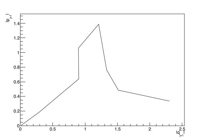
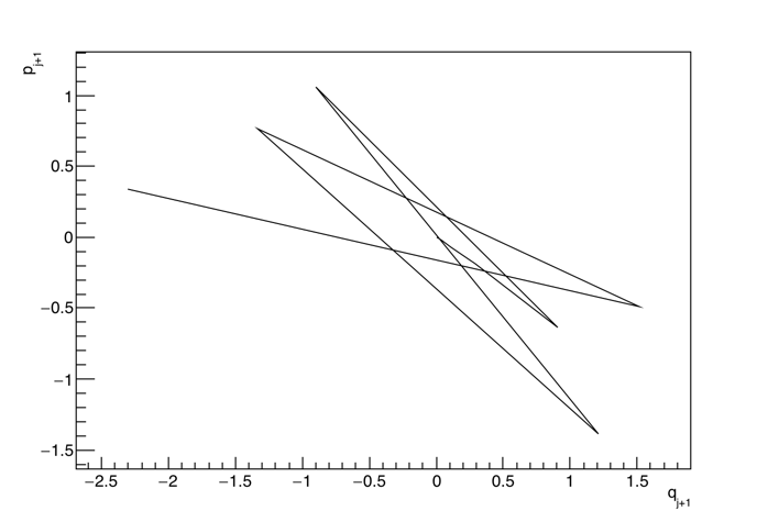
Figure 1: $|p_{j+1}|$ vs. $|q_{j+1}|$ and $p_{j+1}$ vs. $q_{j+1}$

for values $q_{1}=0.00000005$ and $p_{1}=0$, which is compatible with results given in [26] for a continuous version. It is easy to see that the curve in [26] is an equivalent continuous version of our representation above. This could be reenacted in terms of the left discrete Hamiltonian.

The discrete flow approach

To obtain a result of the Hamilton–Jacobi equation applied to our optimal control problem, we need to solve the generating function $S_{d}^{j}$ or equivalently, $DS_{d}^{j}$. For this, we use equation (4), whose solution for this particular example is

$$DS^{j+1}_{d}=- q_{j}^{3}+q_{j}-q_{j+1}\pm$$

$$\sqrt{q_{j}^{6}-2q_{j}^{4}+2q_{j}^{3}q_{j+1}+2hDS^{j}_{d}+2q_{j}^{2}-2q_{j}q_{j+1}+q_{j+1}^{2}}$$ (65)

Solving recurrently this expression for initial values $q_{1}=0.00000005,q_{2}=1.5*10^{-7}$ and $DS^{1}_{d}=0$ and a value $h=0.0001$, we obtain a graphic for values of $DS_{d}^{j}$ versus $q_{j}$ and for the absolute values of $|DS_{d}^{j}|$ versus $|q_{j}|$.

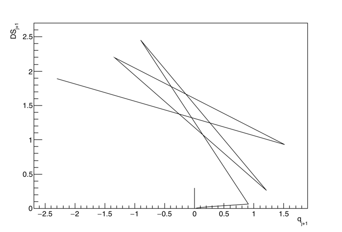
Figure 2: $|DS^{j+1}_{d}|$ vs. $|q_{j+1}|$ and $DS^{j+1}_{d}$ vs. $q_{j+1}$

The graphic on the right hand side shows that the phase space obtained for $(DS^{j+1}_{d},q_{j+1})$ where $DS^{j+1}_{d}$ plays the role of $p_{j+1}$ is equivalent to the phase space $(p_{j+1},q_{j+1})$ given by the right discrete Hamilton equations (1). Indeed, the form and variation of the variable are the same but there is a displacement along the $y$ axis because of constant terms in (4) that produce this shift.

The graphic on the left hand side shows a similar behavior between the absolute value phase space $(|DS^{j+1}_{d}|,|q_{j+1}|)$ and the absolute value phase space $(|p_{j+1}|,|q_{j+1}|)$ from (1). Indeed, there is a linear growth of $|DS^{j+1}_{d}|$ and $|p_{j+1}|$ between values $|q_{j+1}|=\{0,0.9\}$ and a peak around $|q_{j+1}|=1$. The discordance between both graphics is rooted in the $y$ axis shift commented for the case on right hand side.

This means that although it is evident that $DS^{j+1}_{d}$ obtained from equation (4) by (4) and $p_{j+1}$ are equivalent, given the representations $DS^{j+1}_{d}$ vs. $q_{j+1}$ and $p_{j+1}$ vs. $q_{j+1}$, the phase shift in the $y$ axis is quite visible in the absolute value phase space.

The next subsection shows that the results obtained through the discrete vector field approach are more accurate and there is no axis shift.

The discrete vector field approach

To apply the discrete vector field approach in our optimal control problem, we need to impose condition (41) for a vector field that reads

$$X_{d}=\sum_{j=1}^{N-1}\left(q_{j}-q_{j}^{3}-p_{j+1}\right)\frac{\partial}{\partial q_{j+1}}+\left((1-3q_{j}^{2})p_{j+1}+q_{j}\right)\frac{\partial}{\partial p_{j}}$$ (66)

and whose projection is

$$X_{d}^{\gamma}=\sum_{j=1}^{N-1}\left(q_{j}-q_{j}^{3}-p_{j+1}\right)\frac{\partial}{\partial q_{j+1}}$$ (67)

We choose a section $\gamma=\{\gamma_{j}(q_{j+1}),\forall j=1,\dots,N-1\}$ and through (41), we obtain the following equation,

$$\left(q_{j}-q_{j}^{3}-p_{j+1}\right)\frac{\partial\gamma_{j}(q_{j+1})}{\partial q_{j+1}}=\left(1-3q_{j}^{2}\right)p_{j+1}+q_{j}$$ (68)

whose solution is

$$\gamma_{j+1}(q_{j+2})=\frac{-\left(\gamma_{j}(q_{j+1})q_{j}^{2}-\gamma_{j}(q_{j+1})+q_{j+1}\right)q_{j}}{\gamma_{j}(q_{j+1})+q_{j+1}-3q_{j}^{2}q_{j+1}}$$ (69)

Solving this expression by imposing initial values $\gamma_{1}=0$, $q_{1}=0.00000005$ and $q_{2}=0.00000005$, we obtain the following values if we represent $|\gamma_{j+1}(x_{j+2})|$ vs. $|q_{j+1}|$ and $\gamma_{j+1}(q_{j+2})$ vs. $q_{j+1}$, we have

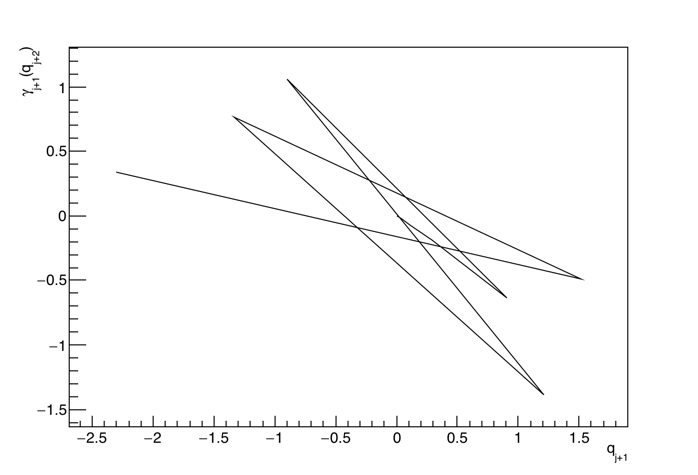
Figure 3: $|\gamma_{j+1}|$ vs. $|q_{j+1}|$ and $\gamma_{j+1}$ vs. $q_{j+1}$.

From these graphics, we can clearly see that there is a good match between the results obtained for $\gamma_{j+1}$ playing the role of the momenta $p_{j+1}$ and the momenta themselves $p_{j+1}$ of the phase space (1). There exists no phase shift in the $y$ axis as it happened in the discrete flow interpretation.

Comparion of methods

From the previous graphics, it is clear that the discrete vector field interpretation seems more accurante than the discrete flow interpretation and the discrete generating function formula (4). To see the accuracy of the discrete Hamiltonian vector field approach, we represent the matching between $\gamma_{j}(q_{j+1})$ representing the role of $|p_{j+1}|$ and $|p_{j+1}|$ from (1).

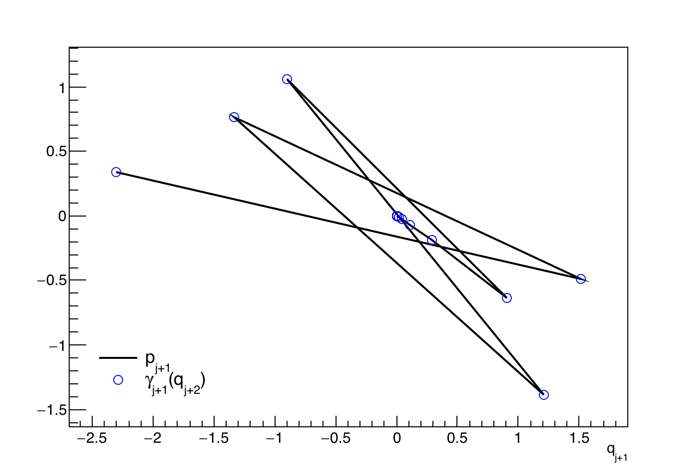
Figure 4: $\gamma_{j+1}(q_{j+2})$ and $p_{j+1}$ vs. $q_{j+1}$

5 Conclusions

In this paper we have proposed two alternative ways of solving a discrete Hamiltonian problem through two different geometric interpretations. The first approach consists of reinterpreting former results available in the literature of discrete Mechanics, by their geometric understanding based on projected flows and the existence of a generating function whose first-order derivative is a Lagrangian submanifold of the discrete phase space. The second approach consists of understanding the discrete dynamics in terms of a discrete vector field whose integral curves are the discrete Hamilton equations. We propose a geometric interpretation by a projected discrete vector field which composed with a Lagrangian submanifold of the discrete phase space provides the dynamics of the complete discrete Hamiltonian vector field. For this matter, we have constructed a discrete Hamiltonian vector field, whose interpretation in the discrete realm is not straightforward. As a byproduct, we obtain two different discrete Hamilton–Jacobi equations. From the first approach we retrieve the discrete Hamilton–Jacobi equation existing in the literature. From the second, we obtain a different Hamilton–Jacobi equation which is proven to be equivalent to the first. An optimal control example compares the accuracy of the two approaches. It is evident that our interpretation in terms of discrete vector fields is more accurate than former theories of discrete Mechanics. Evidency is given through numerical computation and graphic results. In this way, this manuscript provides an alternative way of obtaining the momenta of a dynamical system through a geometric and discrete Hamilton–Jacobi theory founded on discrete Hamiltonian vector fields.

Appendix A

The left discrete action is

$$S_{d}^{j+1}(q_{j+1})-S_{d}^{j}(q_{j})=-p_{j}q_{j}-H_{d}^{-}(p_{j},q_{j+1}).$$ (70)

If we derivate with respect to $q_{j}$, we have that $p_{j}=DS_{d}^{j}(q_{j})$. Introducing this in the expression, we obtain the left discrete Hamilton–Jacobi equation.

$$S_{d}^{j+1}(q_{j+1})-S_{d}^{j}(q_{j})+DS_{d}^{j}(q_{j})q_{j}+H_{d}^{-}(DS_{d}^{j}(q_{j}),q_{j+1})=0$$ (71)

The left discrete Hamilton–Jacobi equation is equivalent to the right discrete Hamilton–Jacobi equation (2.3). Their equivalence gives us the relationship between the right and left Hamiltonians,

$$H_{d}^{-}(p_{j},q_{j+1})+p_{j}q_{j}=H_{d}^{+}(q_{j},p_{j+1})-p_{j+1}q_{j+1}$$ (72)

The discrete flow interpretation can be reenacted for the left formalism.

Appendix B

The left discrete vector field is constructed with the left Hamilton equations (2.3). In this way,

$$X_{d}^{-}=\sum_{i=1}^{N-1}\left(-D_{2}H_{d}^{-}(q_{j+1},p_{j})\frac{\partial}{\partial q_{j}}-D_{1}H_{d}^{-}(q_{j+1},p_{j})\frac{\partial}{\partial p_{j+1}}\right)$$ (73)

Equivalently, the Hamilton–Jacobi theory can be interpreted through the left vector field as performed in (41) for the right case. The projected vector field is

$$X_{d}^{-}=-\sum_{j=1}^{N-1}D_{2}H_{d}^{-}(q_{j+1},p_{j})\frac{\partial}{\partial q_{j}}$$ (74)

Choosing a section $\gamma=\{\gamma_{j}(q_{j+1}),j=1,\dots,N-1\}$ and imposing (41), we arrive at

$$D_{2}H_{d}^{-}(q_{j+1},p_{j})\frac{\partial\gamma_{j+1}}{\partial q_{j}}=D_{1}H_{d}^{-}(q_{j+1},p_{j})$$ (75)

This Hamilton-Jacobi equation is equivalent to the right discrete Hamilton–Jacobi equation in (42). Furthermore, this equation can also be obtained through the left discrete flow interpretation in terms of generating functions.

References

- [1] R. Abraham, J.E. Marsden, Foundations of Mechanics, 2nd Ed. Benjamin–Cumming, Reading, 1978.
- [2] V.I. Arnold, Mathematica methods of Classical Mechanics, Graduate Texts in Mathematics 60, Springer–Verlag, Berlin, 1978.
- [3] V.I. Arnold, Dynamical Systems III, Enciclopaedia of Mathematical Sciences, Springer-Verlag 1988.
- [4] A.M. Bloch, Asymptotic Hamiltonian Dynamics: the Toda Lattice, the three wave interaction and nonholonomic Chaplygin sleigh, Physica D Nonlinear phenomena 141, 297–315 (2000).
- [5] M. Crampin, On the differential geometry of the Euler–Lagrange equations and the inverse problem of Lagrangian dynamics. J. Phys. A: Math. Gen. 14, 2567–2575 (1981).
- [6] J. Cresson, F. Pierret, Continuous versus discrete structures II- discrete Hamiltonian systems and Helmholtz condition, arXiv preprint: 1411.7117 (2015).
- [7] P. Dirac, Lectures on Quantum Mechanics, Dover Pul. Inc. 2001.
- [8] N.A. Elnatanov, J. Schiff, The Hamilton–Jacobi difference equation, Functional differential equations 3, 279–286 (1996).
- [9] M. Gotay, J.M. Nester, Presymplectic Lagrangian systems I. The constraint algorithm and the equivalence theorem, Annals de l’IHP, Section A, 30, 129–142 (1979).
- [10] M. Gotay, J.M. Nester, G. Hinds, Presymplectic manifolds and the Dirac-Bergman theory of constraints, J. Math. Phys. 19, 2388 (1978).
- [11] H. Goldstein, Mecánica Clásica, 4a Ed. Aguilar SA Madrid, 1979.
- [12] H. Goldstein, C.P Poole, J.L. Safko, Classical Mechanics, 3rd. ed., Addison-Wesley, Reading, MA, 2001.
- [13] V.M. Guibot, A.M. Bloch, Discrete variational principles and Hamilton–Jacobi theory for mechanical systems and optimal control problems, arXiv preprint: math/0409296 (2004).
- [14] B.W. Jordan, E. Polak, Theory of a class of discrete optimal control systems, Journal of Electronics and Control 17, 694–711 (1964).
- [15] T.W. Kibble, F.H. Berkshire, Classical Mechanics, Imperial College Press, London, 5th Ed., 2004.
- [16] J. Klein, Operateurs differéntielles sur les variétés puesque tangentes C.R. Acad. Sci. Paris 257, 2392–2394 (1963).
- [17] S. Lall, M. West, Discrete variational Hamiltonian Mechanics, J. Math. A: Math. Gen. 39, 5509–5519 (2006).
- [18] M. de León, P.R. Rodrigues, Methods of Differential Geometry in Analytical Mechanics, Mathematical Studies, North–Holland 158, 1989.
- [19] M. de León, C. Sardón, A geometric Hamilton–Jacobi theory on Nambu–Poisson manifolds, arXiv preprint: 1604.08904, (2016).
- [20] M. de León, C. Sardón, Cosymplectic and contact structures to resolve time-dependent and dissipative hamiltonian systems, arXiv preprint: 1607.01239, (2016).
- [21] J.E. Marsden, Lectures on Mechanics, Cambridge University Press, 1992.
- [22] J.E. Marsden, M. West, Discrete Mechanics and variational integrators, Acta Numerica 10, Cambridge. Cambridge University Press, 2001.
- [23] R.E. Mickens, Difference equation: theory and applications, Chapman and Hall, CRC, 1991.
- [24] T. Ohsawa, A. M. Bloch, M. Leok, Discrete Hamilton–Jacobi theory, SIAM J. Control Optim. 49, 1829–1856 (2011).
- [25] D. Richtmeyer, K.W. Morton, Difference methods for initial value problems, 2nd Ed. Wiley, NY (1967).
- [26] N. Sakamoto, A.J. Van der Schaft, Analytical approximation methods for the stabilizing solution of the Hamilton–Jacobi equation, IEEE Transactions on automatic control, 53, 2335–2350 (2008).
- [27] G. Teschi, Jacobi operators and completely integrable nonlinear lattices, Mathematical Surveys and Monographs 72, Amer. Math. Soc. Providence, 2000.