Zheng Sun, José A. Carrillo and Chi-Wang Shu

Abstract

We consider a class of time dependent second order partial differential equations governed by a decaying entropy. The solution usually corresponds to a density distribution, hence positivity (non-negativity) is expected. This class of problems covers important cases such as Fokker-Planck type equations and aggregation models, which have been studied intensively in the past decades. In this paper, we design a high order discontinuous Galerkin method for such problems. If the interaction potential is not involved, or the interaction is defined by a smooth kernel, our semi-discrete scheme admits an entropy inequality on the discrete level. Furthermore, by applying the positivity-preserving limiter, our fully discretized scheme produces non-negative solutions for all cases under a time step constraint. Our method also applies to two dimensional problems on Cartesian meshes. Numerical examples are given to confirm the high order accuracy for smooth test cases and to demonstrate the effectiveness for preserving long time asymptotics.

Keywords: discontinuous Galerkin method, positivity-preserving, entropy-entropy dissipation relationship, nonlinear parabolic equation, gradient flow

1 Introduction

In this paper, we propose a discontinuous Galerkin method for solving the initial value problem,

$$\left\{\begin{aligned} &\partial_{t}\rho=\nabla\cdot\left(f(\rho)\nabla(H^{\prime}(\rho)+V(\mathbf{x})+W\ast\rho)\right),\quad\mathbf{x}\in\Omega\subset\mathbb{R}^{d},\quad t>0,\\ &\rho(\mathbf{x},0)=\rho_{0}(\mathbf{x}).\\ \end{aligned}\right.$$ (1.1)

Here $\rho=\rho(\mathbf{x},t)\geq 0$ is a time-dependent density. $H^{\prime}$ is strictly increasing and $W(\mathbf{x})=W(-\mathbf{x})$ is symmetric. We assume $f(\rho)\geq 0$ and it attains zero if and only if $\rho=0$. $f$ either increases strictly with respect to $\rho$, or it satisfies the property $\frac{f(\rho)}{\rho}\leq C$ for some fixed constant $C$.

Our concern for (1.1) arises from two typical scenarios. The first case is on nonlinear (possibly degenerate) parabolic equations,

$$\partial_{t}\rho=\nabla\cdot\left(f(\rho)\nabla\left(H^{\prime}(\rho)+V(\mathbf{x})\right)\right).$$ (1.2)

Many classic problems can be included in this setting, such as the heat equation, the porous media equation, the Fokker-Planck equation and so on.

In the second case, several authors take the interaction term $W\ast\rho$ into account, while imposing $f(\rho)=\rho$. Hence the equation takes the form of a continuity equation, and the velocity field is determined by the gradient of a potential function.

$$\partial_{t}\rho=\nabla\cdot\left(\rho\mathbf{u}\right),\qquad\mathbf{u}=\nabla\xi=\nabla\left(H^{\prime}(\rho)+V(x)+W\ast\rho\right).$$ (1.3)

Here, $H$ is a density of internal energy, $V$ is a confinement potential, and $W$ is an interaction potential. It is used to model, for example, interacting gases [16, 43], granular flows [4, 5] and aggregation behaviors in biology [40, 42]. This equation is also related with the gradient flow for the Wasserstein metric on the space of probability measures [2].

Both of the problems (1.2) and (1.3) can be formulated under the framework of (1.1). It has an underlying structure associated with the entropy functional,

$$E=\int_{\Omega}H(\rho(\mathbf{x}))d\mathbf{x}+\int_{\Omega}V(\mathbf{x})\rho(\mathbf{x})d\mathbf{x}+\frac{1}{2}\int_{\Omega}\int_{\Omega}W(\mathbf{x}-\mathbf{y})\rho(\mathbf{x})\rho(\mathbf{y})d\mathbf{x}d\mathbf{y}.$$ (1.4)

One can show that at least for classical solutions,

$$\frac{d}{dt}E(\rho)=-\int_{\Omega}f(\rho)|\mathbf{u}|^{2}d\mathbf{x}:=-I(\rho)\leq 0.$$ (1.5)

Here $\mathbf{u}$ is defined as that in (1.3) and $I$ is referred to as the entropy dissipation.

Indeed, (1.5) has provided much insight into the problem and has helped people to study the dynamics of (1.2) and (1.3), see, for example [15, 16, 43]. Hence it is desirable to develop numerical schemes mimicking a similar entropy-entropy dissipation relationship in the discrete sense.

Another challenge for developing the numerical schemes is to ensure the non-negativity of the numerical density without violating the mass conservation. It is not only for the preservation of physical meanings, but also for the well-posedness of the initial value problem. For example, in (1.3), the entropy may not necessarily decay if $\rho$ admits negative values.

Numerical schemes addressing both of these concerns have been studied intensively very recently. In [6], the authors designed a second order finite volume scheme for (1.2). Later on, a direct discontinuous Galerkin method has been proposed by Liu and Wang in [37]. Their scheme achieves high order accuracy but the preservation of non-negativity only holds for limited cases. As for (1.3), a variety of numerical methods have been developed, including a mixed finite element method [8], a finite volume method [12], a particle method [14], a method of evolving diffeomorphisms [17] and a blob method [22] (for $H=0$, $V=0$).

In this paper, we design a high order discontinuous Galerkin (DG) method for (1.1), which covers both (1.2) and (1.3). The DG method is a class of finite element methods using spaces of discontinuous piecewise polynomials and is especially suitable for solving hyperbolic conservation laws. Coupled with strong stability preserving Runge-Kutta (SSP-RK) time discretization and suitable limiters (the so-called RKDG method, developed by Cockburn et al. in [26, 25, 24, 23, 27]), the method captures shocks effectively and achieves high order accuracy in smooth regions [29]. The method has also been generalized for problems involving diffusion and higher order derivatives, for example, the local DG method [3, 28], the ultra-weak DG method [21] and the direct DG method [38].

Our idea is to formally treat (1.1) as a classical conservation law and apply the techniques there to overcome the challenges. The main ingredients for our schemes are:

1. Legendre-Gauss-Lobatto quadrature rule for numerical integration,

2. positivity-preserving limiter with SSP-RK time discretization.

The quadrature is used to stabilize the semi-discrete scheme. Such approach has already been studied in different contexts, such as in spectral collocation methods [34] and in nodal discontinuous Galerkin methods [35]. Recently, based on the methodology established in [11, 31, 32], Chen and Shu proposed a unified framework for designing entropy stable DG scheme for hyperbolic conservation laws using suitable quadrature rules [20]. Their approach is also related with the summation-by-part technique in finite difference methods. The positivity-preserving limiter with provable high order accuracy is firstly designed by Zhang and Shu in [45] to numerically ensure the maximum principle of scalar hyperbolic conservation laws. Then the methodology has been generalized for developing the bound-preserving schemes for various systems. We refer to [46] and the references therein for more details. Our approach of implementing the positivity-preserving limiter for parabolic problems is mainly inspired by the recent work of Zhang on compressible Navier-Stokes equation [44], in which the author considers the conservative form of the problem and introduces the diffusion flux to handle the second order derivatives.

Based on these techniques, we propose a discontinuous Galerkin scheme for (1.1) such that

1. the semi-discrete scheme satisfies an entropy inequality for smooth $W$,

2. the fully discretized scheme is positivity-preserving.

Our method also has other desired properties. It achieves high order accuracy, conserves the total mass and preserves numerical steady states. Special care is needed for the case of non-smooth interaction potential, due to the fact that one should adopt exact integration to calculate the convolution, see [12], as the Gauss-Lobatto quadrature is no longer accurate.

The remaining part of the paper is organized as follows. In Section 2, we design the numerical method for one dimensional problems. We firstly introduce the notations and briefly discuss our motivation on deriving the scheme. Then it follows with the semi-discrete scheme and the discrete entropy inequality. The next part is on the time discretization and the positivity-preserving property of the fully discretized scheme. Finally we outline the matrix formulation and the algorithm flowchart. Section 3 is organized similarly for two dimensional problems on Cartesian meshes, while the implementation details are omitted. Then in Section 4 and Section 5, we present numerical examples for one dimensional and two dimensional problems respectively. Finally conclusions are drawn in Section 6.

2 Numerical method: one dimensional case

2.1 Notations and motivations

For now, we focus on the one dimensional case of (1.1)

$$\left\{\begin{aligned} &\partial_{t}\rho=\partial_{x}\big{(}f(\rho)\partial_{x}(H^{\prime}(\rho)+V(x)+W\ast\rho)\big{)},\quad x\in\Omega\subset\mathbb{R},\quad t>0,\\ &\rho(x,0)=\rho_{0}(x).\\ \end{aligned}\right.$$

In general, the problem can be either defined on a connected compact domain with proper boundary conditions, or it can involve the whole real line with solutions vanishing at the infinity. In our numerical scheme, we will always choose $\Omega$ to be a connected interval. For simplicity, the periodic or compactly supported boundary conditions are applied. But we remark that our approach can be extended to more general types of boundary conditions, for example, with zero-flux boundaries.

Let $I_{i}=(x_{i-\frac{1}{2}},x_{i+\frac{1}{2}})$ and $I=\cup_{i=1}^{N}I_{i}$ be a regular partition of the domain $\Omega$. Denote $h_{i}=x_{i+\frac{1}{2}}-x_{i-\frac{1}{2}}$ and $h=\max_{i}h_{i}$. We will seek a numerical solution in the discontinuous piecewise polynomial space,

$$V_{h}=\{v_{h}:v_{h}\big{|}_{I_{i}}\in P^{k}(I_{i}),\text{for }x\in I_{i},i=1,\dots,N\}.$$

Here $P^{k}(I_{i})$ is the space of $k$-th order polynomials on $I_{i}$. Note that the functions in $V_{h}$ can be double-valued at the cell interfaces. Hence the notations $v_{h}^{+}$ and $v_{h}^{-}$ are introduced for the right limit and the left limit of $v_{h}$. For a function $s=s(\rho)$ or $s=s(\rho,x)$, we denote by $s_{h}=s(\rho_{h})$ or $s_{h}=s(\rho_{h},x)$ respectively. Furthermore, the notation $s_{h}^{+}$ stands for $s(\rho_{h}^{+})$ or $s(\rho_{h}^{+},x)$, and $s^{-}_{h}$ stands for $s(\rho_{h}^{-})$ or $s(\rho_{h}^{-},x)$.

To define the DG method, we split the original problem into the following system,

$$\partial_{t}\rho =\partial_{x}(f(\rho)u),$$

$$u =\partial_{x}\xi,$$

$$\xi =H^{\prime}(\rho)+V+W\ast\rho.$$

By applying the DG approximation, we obtain the following scheme as a rudiment. We seek $\rho_{h},u_{h}\in V_{h}$, such that for any test function $\varphi_{h},\psi_{h}\in V_{h}$,

$$\int_{I_{i}}(\partial_{t}\rho_{h})\varphi_{h}dx =-\int_{I_{i}}f_{h}u_{h}\partial_{x}\varphi_{h}dx+\widehat{fu}_{i+\frac{1}{2}}(\varphi_{h})_{i+\frac{1}{2}}^{-}-\widehat{fu}_{i-\frac{1}{2}}(\varphi_{h})_{i-\frac{1}{2}}^{+},$$ (2.2a)

$$\int_{I_{i}}u_{h}\psi_{h}dx =-\int_{I_{i}}\xi_{h}\partial_{x}\psi_{h}dx+\widehat{\xi}_{i+\frac{1}{2}}(\psi_{h})_{i+\frac{1}{2}}^{-}-\widehat{\xi}_{i-\frac{1}{2}}(\psi_{h})_{i-\frac{1}{2}}^{+}.$$ (2.2b)

Here $\xi_{h}=H^{\prime}_{h}+V+\int_{\Omega}W(x-y)\rho_{h}(y)dxdy$, while $\widehat{fu}$ and $\widehat{\xi}$ are numerical fluxes.

By setting $\varphi_{h}(x)=1_{I_{i}}(x)$, one will get the following evolution equation for the cell average of $(\rho_{h})_{i}$, which is denoted by $(\bar{\rho}_{h})_{i}$.

$$\frac{d}{dt}\left(\bar{\rho}_{h}\right)_{i}=\frac{\widehat{fu}_{i+\frac{1}{2}}-\widehat{fu}_{i-\frac{1}{2}}}{h_{i}}.$$ (2.3)

This is very similar to that in hyperbolic conservation laws. In particular, for $k=0$ and $u\equiv 1$, by using the so called monotone flux, (2.3) will become a monotone scheme, which satisfies many desirable properties.

In order to achieve an entropy-entropy dissipation relationship as that for the exact solution, one may hope to set $\varphi_{h}=\xi_{h}$ in (2.2a) and $\psi_{h}=u_{h}f_{h}$ in (2.2b). Unluckily, neither of them falls into the test function space. A natural attempt is to use the usual $L^{2}$ projection to enforce this property, as that in [37]. However, the projection will change the values at the cell interfaces, and the desired form in (2.3) will be violated. This will cause trouble when one seeks to preserve the non-negativity of the solution. Inspired by the recent work of Chen and Shu in [20], we introduce a suitable quadrature to overcome this difficulty. Moreover, the Gauss-Lobatto quadrature is used to preserve the values at the cell ends.

Let us denote by $\{x^{r}_{i}\}_{r=1}^{k+1}$ the $k+1$ Gauss-Lobatto quadrature points on $I_{i}$ and $\{w_{r}\}_{r=1}^{k+1}$ the $k+1$ Gauss-Lobatto quadrature weights on $[-1,1]$. In particular $x^{1}_{i}=x^{+}_{i-\frac{1}{2}}$ and $x^{k+1}_{i}=x^{-}_{i+\frac{1}{2}}$. On each cell $I_{i}$, the operator $\mathcal{I}$ returns the $k$-th order polynomial interpolating at $\{x^{r}_{i}\}_{r=1}^{k+1}$. We will use the notation

$$\overset{\sim}{\int_{I_{i}}}\eta\zeta dx=\frac{h_{i}}{2}\sum_{r=1}^{k+1}w_{r}\eta(x_{i}^{r})\zeta(x_{i}^{r})$$

and

$$\overset{\sim}{\int_{I_{i}}}\eta\partial_{x}\zeta dx=\frac{h_{i}}{2}\sum_{r=1}^{k+1}w_{r}\eta(x_{i}^{r})(\partial_{x}\mathcal{I}\zeta)(x_{i}^{r})$$

for the Gauss-Lobatto quadrature. As a convention, $\overset{\sim}{\int_{\Omega}}$ stands for $\sum_{i}\overset{\sim}{\int_{I_{i}}}$.

We will finally come to the fully discretized scheme, for which we denote by $\tau$ the time step length and $\lambda_{i}=\frac{\tau}{h_{i}}$.

2.2 Semi-discrete scheme and entropy inequality

Our scheme is to replace the integrals in (2.2) by the Gauss-Lobatto quadrature. In other words, we seek $\rho_{h},u_{h}\in{V_{h}}$, such that for any test functions $\varphi_{h},\psi_{h}\in V_{h}$,

$$\overset{\sim}{\int_{I_{i}}}(\partial_{t}\rho_{h})\varphi_{h}dx =-\overset{\sim}{\int_{I_{i}}}f_{h}u_{h}\partial_{x}{\varphi_{h}}dx+\widehat{fu}_{i+\frac{1}{2}}(\varphi_{h})_{i+\frac{1}{2}}^{-}-\widehat{fu}_{i-\frac{1}{2}}(\varphi_{h})_{i-\frac{1}{2}}^{+},$$ (2.4a)

$$\overset{\sim}{\int_{I_{i}}}u_{h}\psi_{h}dx =-\overset{\sim}{\int_{I_{i}}}\xi_{h}\partial_{x}\psi_{h}dx+\widehat{\xi}_{i+\frac{1}{2}}(\psi_{h})_{i+\frac{1}{2}}^{-}-\widehat{\xi}_{i-\frac{1}{2}}(\psi_{h})_{i-\frac{1}{2}}^{+}.$$ (2.4b)

Here, when the interaction potential $W$ is smooth, we set

$$\xi_{h}=\xi_{h}(\rho_{h},x)=H^{\prime}_{h}+V+\overset{\sim}{\int_{\Omega}}W(x-y)\rho_{h}(y)dy.$$

While for non-smooth $W$, the quadrature may not achieve sufficient accuracy of the convolution. Hence the exact integration is applied

$$\xi_{h}=\xi_{h}(\rho_{h},x)=H^{\prime}_{h}+V+\int_{\Omega}W(x-y)\rho_{h}(y)dy.$$

The numerical fluxes are chosen in the following way,

$$\widehat{\xi} =\frac{1}{2}(\xi_{h}^{+}+\xi_{h}^{-}),$$

$$\widehat{fu} =\frac{1}{2}(f_{h}^{+}u_{h}^{+}+f_{h}^{-}u_{h}^{-})+\frac{\alpha}{2}(g_{h}^{+}-g_{h}^{-}),\quad\alpha=\max\{|u^{+}_{h}|,|u^{-}_{h}|\},$$

with $g(\rho)=f(\rho)$ if $f$ is increasing and $g(\rho)=C\rho$ if $\frac{f(\rho)}{\rho}\leq C$. $\widehat{\xi}$ is the central flux. When $f(\rho)=\rho$, one can choose $g(\rho)=\rho$ and $\widehat{fu}$ is the Lax-Friedrich flux.

Remark 2.1.

Although we formally require that $\varphi_{h}$ and $\psi_{h}$ are taken from the finite element space, our scheme (2.4) actually can not distinguish a function from its interpolation polynomial at the Gauss-Lobatto points. Hence, (2.4) will also hold for “test functions” outside $V_{h}$. This facilitates our proof of the discrete entropy inequality. This fact can also be justified through the matrix formulation, which is presented in Section 2.4.

This semi-discrete scheme satisfies the following entropy inequality.

Theorem 2.1.

For smooth interaction kernel $W$, assume that the semi-discrete scheme (2.4) has a solution, then it satisfies a similar entropy-entropy dissipation relationship, as that in (1.5), given by

$$\frac{d}{dt}\tilde{E}\leq-\tilde{I},$$

where

$$\tilde{E}=\overset{\sim}{\int_{\Omega}}H(\rho_{h})dx+\overset{\sim}{\int_{\Omega}}V\rho_{h}dx+\frac{1}{2}\overset{\sim}{\int_{\Omega}}\overset{\sim}{\int_{\Omega}}W(x-y)\rho_{h}(x)\rho_{h}(y)dxdy$$

is the discrete entropy and

$$\tilde{I}=\overset{\sim}{\int_{\Omega}}f_{h}|u_{h}|^{2}dx$$

is the associated discrete entropy dissipation.

Indeed, one can choose larger $\alpha_{i+\frac{1}{2}}$ in the Lax-Friedrich flux. This will bring in extra numerical dissipation and the entropy inequality will still hold. Moreover, if $\alpha_{i+\frac{1}{2}}>0$ for all $i$ and the semi-discrete scheme (2.4) achieves a non-negative stationary state $\rho_{h}$, then $\rho_{h}$ is continuous and the piecewise polynomial interpolation of $\xi_{h}$ is constant in each connected component $J$ of the support of $\rho_{h}$, which is defined by $J=\cup_{i\in\Lambda}I_{i}$ for certain set of consecutive indices $\Lambda$ where $\rho_{h}>0$.

Proof.

Using the symmetry of $W$, we have

$$\begin{split}&\frac{d}{dt}\frac{1}{2}\overset{\sim}{\int_{\Omega}}\overset{\sim}{\int_{\Omega}}W(x-y)\rho_{h}(x)\rho_{h}(y)dxdy\\ =&\frac{1}{2}\overset{\sim}{\int_{\Omega}}\partial_{t}\rho_{h}(x)\left(\overset{\sim}{\int_{\Omega}}W(x-y)\rho_{h}(y)dy\right)dx+\frac{1}{2}\overset{\sim}{\int_{\Omega}}\partial_{t}\rho_{h}(y)\left(\overset{\sim}{\int_{\Omega}}W(x-y)\rho_{h}(x)dx\right)dy\\ =&\overset{\sim}{\int_{\Omega}}\partial_{t}\rho_{h}(x)\left(\overset{\sim}{\int_{\Omega}}W(x-y)\rho_{h}(y)dy\right)dx.\end{split}$$

Hence,

$$\begin{split}\frac{d}{dt}\tilde{E}&=\overset{\sim}{\int_{\Omega}}\partial_{t}\rho_{h}(x)\left(H^{\prime}_{h}+V+\overset{\sim}{\int_{\Omega}}W(x-y)\rho_{h}(y)dy\right)dx\\ &=\overset{\sim}{\int_{\Omega}}\partial_{t}\rho_{h}\xi_{h}dx=\sum_{i}\overset{\sim}{\int_{I_{i}}}\partial_{t}\rho_{h}\mathcal{I}(\xi_{h})dx\\ &=\sum_{i}\left(-\overset{\sim}{\int_{I_{i}}}\mathcal{I}(f_{h}u_{h})\partial_{x}\mathcal{I}(\xi_{h})dx+\widehat{fu}_{i+\frac{1}{2}}(\xi_{h})_{i+\frac{1}{2}}^{-}-\widehat{fu}_{i-\frac{1}{2}}(\xi_{h})_{i-\frac{1}{2}}^{+}\right).\end{split}$$

Note $\mathcal{I}(f(\rho_{h})u_{h})\partial_{x}\mathcal{I}(\xi_{h})$ is a polynomial of degree $2k-1$ and the Gauss-Lobatto quadrature with $k+1$ points is exact. Hence we can replace the quadrature with the exact integral and integrate by parts. Then we obtain

$$\begin{split}\frac{d}{dt}\tilde{E}=\sum_{i}&\left(-\int_{I_{i}}\mathcal{I}(f_{h}u_{h})\partial_{x}\mathcal{I}(\xi_{h})dx+\widehat{fu}_{i+\frac{1}{2}}(\xi_{h})_{i+\frac{1}{2}}^{-}-\widehat{fu}_{i-\frac{1}{2}}(\xi_{h})_{i-\frac{1}{2}}^{+}\right)\\ =\sum_{i}&\bigg{(}\int_{I_{i}}(\partial_{x}\mathcal{I}(f_{h}u_{h}))\mathcal{I}(\xi_{h})dx-(f_{h}u_{h}\xi_{h})_{i+\frac{1}{2}}^{-}\\ \qquad\qquad&+(f_{h}u_{h}\xi_{h})_{i-\frac{1}{2}}^{+}+\widehat{fu}_{i+\frac{1}{2}}(\xi_{h})_{i+\frac{1}{2}}^{-}-\widehat{fu}_{i-\frac{1}{2}}(\xi_{h})_{i-\frac{1}{2}}^{+}\bigg{)}.\\ \end{split}$$

By using the same trick, we change the exact integral back to the Gauss-Lobatto quadrature, and apply the scheme (2.4b) to obtain

$$\frac{d}{dt}\tilde{E}= \sum_{i}\left(\overset{\sim}{\int_{I_{i}}}\xi_{h}\partial_{x}(f_{h}u_{h})dx-(f_{h}u_{h}\xi_{h})_{i+\frac{1}{2}}^{-}+(f_{h}u_{h}\xi_{h})_{i-\frac{1}{2}}^{+}+\widehat{fu}_{i+\frac{1}{2}}(\xi_{h})_{i+\frac{1}{2}}^{-}-\widehat{fu}_{i-\frac{1}{2}}(\xi_{h})_{i-\frac{1}{2}}^{+}\right)$$

$$= \sum_{i}\bigg{(}-\overset{\sim}{\int_{I_{i}}}f_{h}|u_{h}|^{2}dx+\widehat{\xi}_{i+\frac{1}{2}}(f_{h}u_{h})_{i+\frac{1}{2}}^{-}-\widehat{\xi}_{i-\frac{1}{2}}(f_{h}u_{h})_{i-\frac{1}{2}}^{+}-(f_{h}u_{h}\xi_{h})_{i+\frac{1}{2}}^{-}$$

$$+(f_{h}u_{h}\xi_{h})_{i-\frac{1}{2}}^{+}+\widehat{fu}_{i+\frac{1}{2}}(\xi_{h})_{i+\frac{1}{2}}^{-}-\widehat{fu}_{i-\frac{1}{2}}(\xi_{h})_{i-\frac{1}{2}}^{+}\bigg{)}$$

$$= -\overset{\sim}{\int_{\Omega}}f_{h}|u_{h}|^{2}dx-\sum_{i}\frac{\alpha_{i+\frac{1}{2}}}{2}[g_{h}]_{i+\frac{1}{2}}[\xi_{h}]_{i+\frac{1}{2}},$$ (2.6)

where the bracket represents the jump, $[g_{h}]=g_{h}^{+}-g_{h}^{-}$. According to our choice of $g$, $\text{sign}[g_{h}]=\text{sign}[\rho_{h}]$. Since $V$ and $W$ are single-valued functions, $[\xi_{h}]=[H^{\prime}(\rho_{h})]$. By using the fact that $H^{\prime}$ is strictly increasing, we have $\text{sign}[\xi_{h}]=\text{sign}[H^{\prime}(\rho_{h})]=\text{sign}[\rho_{h}]$. Therefore $\sum_{i}\frac{\alpha_{i+\frac{1}{2}}}{2}[g]_{i+\frac{1}{2}}[\xi_{h}]_{i+\frac{1}{2}}\geq 0$, which completes the proof of the first claim.

It is easy to see that the entropy inequality will hold as long as the coefficients $\alpha_{i+\frac{1}{2}}$ are non-negative. Let us assume now that $\alpha_{i+\frac{1}{2}}>0$ for all $i$ and $\rho_{h}$ is a non-negative stationary state of the semi-discrete scheme (2.4), namely

$$\frac{d}{dt}\tilde{E}=0.$$

Then from (2.2) we deduce that both terms in the right-hand side must vanish, that is

$$\sum_{i}\overset{\sim}{\int_{I_{i}}}f_{h}|u_{h}|^{2}dx=\sum_{i}\frac{\alpha_{i+\frac{1}{2}}}{2}[g_{h}]_{i+\frac{1}{2}}[\xi_{h}]_{i+\frac{1}{2}}=0\,.$$

Therefore each term in the summations will be zero. On the one hand, if $\alpha_{i+\frac{1}{2}}>0$, then $[g_{h}]_{i+\frac{1}{2}}[\xi_{h}]_{i+\frac{1}{2}}=0$ and hence $[\rho_{h}]_{i+\frac{1}{2}}=0$. It holds for all $i$, which means the jumps of $\rho_{h}$ vanish on all the cell interfaces. This implies the continuity of $\rho_{h}$. On the other hand, in the interval $J$ we deduce that $u_{h}=0$ due to the positivity of $f_{h}$ implied by the positivity of $\rho_{h}$ and its definition. Hence for all $i\in\Lambda$, by using (2.4b), one can obtain

$$\begin{split}\int_{I_{i}}\partial_{x}(\mathcal{I}\xi_{h})\mathcal{I}\psi_{h}dx&=-\int_{I_{i}}\mathcal{I}\xi_{h}\partial_{x}(\mathcal{I}\psi_{h})dx+(\xi_{h}\psi_{h})_{i+\frac{1}{2}}^{-}-(\xi_{h}\psi_{h})_{i-\frac{1}{2}}^{+}\\ &=-\overset{\sim}{\int_{I_{i}}}\xi_{h}\partial_{x}\psi_{h}dx+\widehat{\xi}_{j+\frac{1}{2}}(\psi_{h})_{i+\frac{1}{2}}^{-}-\widehat{\xi}_{i+\frac{1}{2}}(\psi_{h})_{i-\frac{1}{2}}^{+}\\ &=0.\end{split}$$

Here $\xi_{h}^{\pm}=\widehat{\xi}$ is guaranteed by the continuity of $\xi_{h}$ (implied by that of $\rho_{h}$). Therefore, $\mathcal{I}\xi_{h}$ is constant on each $i\in\Lambda$. Due to the fact that $\xi_{h}$ is continuous globally, all these constants must be the same and the piecewise polynomial interpolation of $\xi_{h}$ is constant on $J$. ∎

2.3 Time discretization and preservation of positivity

The semi-discrete scheme itself does not guarantee the positivity of the numerical solution. If no special treatment is applied, one may produce nonsense density with negative values and the problem can become illposed. Hence we adopt the methodology developed by Zhang and Shu in [45], which enforces the positivity of the solution without violating the mass conservation. Their idea is to incorporate a positivity-preserving limiter into the strong stability preserving Runge-Kutta (SSP-RK) time discretization. Under certain time step constraints, each Euler forward step preserves the positivity of the cell average (referred to as the weak positivity in the literature). Then one can scale the solution, without affecting spatial accuracy, to ensure the point-wise non-negativity. SSP-RK time discretization will preserve the non-negativity of the solution in the Euler forward steps.

2.3.1 First order Euler forward in time

Let us firstly consider the Euler forward time stepping. We use the superscript “pre” for the solution obtained by Euler forward method before applying the positivity-preserving limiter. The time discretization of (2.4a) becomes

$$\overset{\sim}{\int_{I_{i}}}\frac{\rho_{h}^{n+1,\textup{pre}}-\rho_{h}^{n}}{\tau}\varphi_{h}dx=-\overset{\sim}{\int_{I_{i}}}f_{h}^{n}u_{h}^{n}\partial_{x}{\varphi_{h}}dx+(\widehat{fu})^{n}_{i+\frac{1}{2}}(\varphi_{h})_{i+\frac{1}{2}}^{-}-(\widehat{fu})^{n}_{i-\frac{1}{2}}(\varphi_{h})_{i-\frac{1}{2}}^{+}.$$ (2.7)

Lemma 2.1.

Suppose $\rho_{h}^{n}(x_{i}^{r})\geq 0$ at the Gauss-Lobatto quadrature points. Then when $\lambda_{i}\leq\min\{(\frac{w_{1}\rho}{fu+\alpha g})_{i-\frac{1}{2}}^{+},(\frac{w_{k+1}\rho}{\alpha g-fu})_{i+\frac{1}{2}}^{-}\}$, the solution $\rho_{h}^{n+1,\textup{pre}}$ obtained from (2.7) satisfies $\left(\bar{\rho}_{h}\right)_{i}^{n+1,\textup{pre}}\geq 0$. Here, in the constraint of $\lambda_{i}$, we consider $\frac{0}{0}:=+\infty$ by convention.

Proof.

We drop all subscripts $h$ in this proof. Take $\varphi=1$ in (2.7), we have

$$\bar{\rho}^{n+1,\textup{pre}}_{i}=\bar{\rho}^{n}_{i}+\lambda_{i}\left({(\widehat{fu})^{n}_{i+\frac{1}{2}}-(\widehat{fu})^{n}_{i-\frac{1}{2}}}\right).$$

Note that $\rho^{n}$ is a polynomial of degree $k$, the Gauss-Lobatto quadrature is exact for evaluating the cell average $\bar{\rho}_{i}^{n}$. More specifically, we have

$$\bar{\rho}_{i}^{n}=\frac{1}{h_{i}}\int_{I_{i}}\rho^{n}dx=\sum_{r=1}^{k+1}\frac{w_{r}}{2}\rho^{n}(x_{i}^{r}).$$

The superscripts $n$ will also be omitted for simplicity in the rest. Hence

$$\bar{\rho}_{i}^{n+1,\textup{pre}}= \sum_{r=2}^{k}\frac{w_{r}}{2}\rho(x^{r}_{i})+\frac{w_{1}}{2}\rho_{i-\frac{1}{2}}^{+}+\frac{w_{k+1}}{2}\rho_{i+\frac{1}{2}}^{-}+\frac{\lambda_{i}}{2}\left((fu)^{+}_{i+\frac{1}{2}}+(fu)^{-}_{i+\frac{1}{2}}+\alpha_{i+\frac{1}{2}}\left(g_{i+\frac{1}{2}}^{+}-g_{i+\frac{1}{2}}^{-}\right)\right)$$

$$-\frac{\lambda_{i}}{2}\left((fu)^{+}_{i-\frac{1}{2}}+(fu)^{-}_{i-\frac{1}{2}}+\alpha_{i-\frac{1}{2}}\left(g_{i-\frac{1}{2}}^{+}-g_{i-\frac{1}{2}}^{-}\right)\right)$$

$$= \sum_{r=2}^{k}\frac{w_{r}}{2}\rho(x^{r}_{i})+\left(\frac{w_{k+1}}{2}\rho^{-}_{i+\frac{1}{2}}+\frac{\lambda_{i}}{2}\left((fu)^{-}_{i+\frac{1}{2}}-\alpha_{i+\frac{1}{2}}g_{i+\frac{1}{2}}^{-}\right)\right)$$

$$+\left(\frac{\omega_{1}}{2}\rho_{i-\frac{1}{2}}^{+}-\frac{\lambda_{i}}{2}\left((fu)^{+}_{i-\frac{1}{2}}+\alpha_{i-\frac{1}{2}}g^{+}_{i-\frac{1}{2}}\right)\right)$$

$$+\frac{\lambda_{i}}{2}\left((fu)^{+}_{i+\frac{1}{2}}+\alpha_{i+\frac{1}{2}}g_{i+\frac{1}{2}}^{+}\right)-\frac{\lambda_{i}}{2}\left((fu)_{i-\frac{1}{2}}^{-}-\alpha_{i-\frac{1}{2}}g_{i-\frac{1}{2}}^{-}\right).$$

The first term is automatically non-negative, since the weights $w_{r}\geq 0$ and the nodal values $\rho(x^{r}_{i})\geq 0$. The positivity of the last two terms is guaranteed by our choice of $\alpha$ and $g$. One only needs $\lambda_{i}\leq\min\{(\frac{w_{1}\rho}{fu+\alpha g})_{i-\frac{1}{2}}^{+},(\frac{w_{k+1}\rho}{\alpha g-fu})_{i+\frac{1}{2}}^{-}\}$ to ensure the second and the third term to be non-negative. (Note that for $\rho_{i-\frac{1}{2}}^{+}$ or $\rho_{i+\frac{1}{2}}^{-}$ being $0$, the corresponding term is also $0$ and there is nothing to impose. Hence we introduce the notation $\frac{0}{0}:=+\infty$.) Therefore $\bar{\rho}^{n+1,\textup{pre}}_{i}\geq 0$ under the prescribed time step constraint. ∎

Remark 2.2.

1. According to the definition of $\alpha$ and $g$, $(\frac{w_{1}\rho}{fu+\alpha g})_{i-\frac{1}{2}}^{+}$ and $(\frac{w_{k+1}\rho}{\alpha g-fu})_{i+\frac{1}{2}}^{-}$ will always be non-negative.

2. Although the original equation can be parabolic, we have incorporated the second order derivative into $u$, such that one can formally treat it as a hyperbolic problem. This technique is introduced by Zhang for the compressible Navier-Stokes equation [44]. In particular, for $f(\rho)=\rho$, one obtains $\lambda_{i}(\alpha\pm u^{\pm})\leq C$, If $u$ is a constant (as that in Example 4.1.1), this is the usual CFL condition. While in general, the bound of $\lambda_{i}$ may scale like $h_{i}$ and it then gives a typical time step restriction for parabolic problems.

Lemma 2.1 tells us an inherent property of the Euler forward scheme. If the solution is non-negative at the previous time step (at the Gauss-Lobatto quadrature points), as long as the time step is smaller than a threshold, the cell average at next time step will remain non-negative. In order to close the loop, one would need to ensure the nodal values at the quadrature points of the next time step are also non-negative. This indeed can be achieved by applying a scaling limiter, which luckily does not affect the spatial accuracy. We refer to [44] for more details.

Lemma 2.2.

Let

$$\rho_{h}^{n+1}(x_{i}^{r})=(\bar{\rho}_{h})_{i}^{n+1,\textup{pre}}+\theta_{i}\left(\rho_{h}^{n+1,\textup{pre}}(x_{i}^{r})-(\bar{\rho}_{h})_{i}^{n+1,\textup{pre}}\right),\qquad\forall r=1,\dots,k+1,$$

with $\theta_{i}=\min\{\frac{(\bar{\rho}_{h})_{i}^{n+1,\textup{pre}}}{(\bar{\rho}_{h})_{i}^{n+1,\textup{pre}}-m_{i}},1\}$ and $m_{i}=\min\{\rho_{h}^{n+1,\textup{pre}}(x_{i}^{r})\}_{r=1}^{k+1}$. Then we have $\rho_{h}^{n+1}(x_{i}^{r})\geq 0,\forall r=1,\dots,k+1$ and $\left(\bar{\rho}_{h}\right)_{i}^{n+1}=\left(\bar{\rho}_{h}\right)_{i}^{n+1,\textup{pre}}$. Furthermore, the interpolation polynomial of $\{\rho_{h}^{n+1}(x_{i}^{r})\}$ on $I_{i}$ satisfies

$$|\rho_{h}^{n+1}(x)-\rho_{h}^{n+1,\textup{pre}}(x)|\leq C_{k}\max_{x\in I_{i}}|\rho(x,t_{n+1})-\rho_{h}^{n+1,\textup{pre}}(x)|,$$

where $\rho(x,t_{n+1})$ is the exact solution at time $t_{n+1}$ and $C_{k}$ is a constant depending only on the polynomial degree $k$.

Remark 2.3.

Our scheme only uses the nodal values at the Gauss-Lobatto quadrature points, hence we only need to ensure the non-negativity at these nodes. One can also squash the solution polynomials so that the solution is non-negative everywhere on the domain. The proof will still go through.

Theorem 2.2.

With the scaling limiter in Lemma 2.2, the Euler forward time discretization of the semi-discrete scheme is positivity-preserving, provided the time step restriction specified in Lemma 2.1 is satisfied.

2.3.2 High order time discretization

The SSP-RK method will be used for time discretization. We refer readers to [33] for more details. Since the time step scales like $\tau=Ch^{2}$, the Euler forward method will be sufficient for piecewise linear elements to achieve overall second order accuracy. For $k=2,3$, we will use the second order SSP-RK scheme

$$\rho_{h}^{(1)} =\rho^{n}_{h}+\tau F(\rho_{h}^{n}),$$ (2.8a)

$$\rho_{h}^{n+1} =\frac{1}{2}\rho_{h}^{n}+\frac{1}{2}\left(\rho_{h}^{(1)}+\tau F(\rho_{h}^{(1)})\right).$$ (2.8b)

For $k=4,5$, the third order SSP-RK scheme is used

$$\rho_{h}^{(1)} =\rho^{n}_{h}+\tau F(\rho_{h}^{n}),$$ (2.9a)

$$\rho_{h}^{(2)} =\frac{3}{4}\rho_{h}^{n}+\frac{1}{4}\left(\rho^{(1)}_{h}+\tau F(\rho_{h}^{(1)})\right),$$ (2.9b)

$$\rho_{h}^{n+1} =\frac{1}{3}\rho_{h}^{n}+\frac{2}{3}\left(\rho_{h}^{(2)}+\tau F(\rho_{h}^{(2)})\right).$$ (2.9c)

The positivity-preserving limiter should be applied immediately after each Euler forward stage. As one can see, the SSP-RK schemes (2.8) and (2.9) can be rewritten as convex combinations of the Euler forward steps. Since each Euler forward step preserves the positivity, the numerical density at the next time level will remain non-negative.

Theorem 2.3.

Consider the SSP-RK time discretization (2.8) and (2.9) of the semi-discrete scheme (2.4). By applying limiters specified in Lemma 2.2, the fully discretized scheme preserves non-negativity as long as the time step restriction in Lemma 2.1 is satisfied.

We also mention several other properties of the fully discretized scheme, whose proofs are omitted. Such properties also hold for two dimensional cases.

1. Mass conservation: $\int_{\Omega}\rho_{h}^{n}(x)dx=\int_{\Omega}\rho_{0}(x)dx$.

2. Preservation of numerical steady states: if the numerical potential $\xi_{h}$ becomes constant on each connected component of the support of $\rho_{h}$, and $\rho_{h}$ vanishes everywhere else, then we have $\rho_{h}^{n+1}=\rho_{h}^{n}$. We remind the readers that the “preservation of steady states” here for the fully discretized scheme is slightly different from that in Theorem 2.1 for the semi-discrete scheme with smooth $W$. But they are related through the profiles of $\rho_{h}$ and $\xi_{h}$.

2.4 Matrix formulation and implementation

At the end of this section, we would like to introduce the matrix formulation of our numerical scheme and outline the flowchart of the algorithm.

2.4.1 Matrix formulation

The derivation of the matrix formulation is similar to that in Section 3.1 of [20]. We refer to that paper for more details.

We omit all the subscripts $h$. Let $\{\zeta_{r}\}_{r=1}^{k+1}$ be the Gauss-Lobatto quadrature points on the reference element $[-1,1]$. We denote by $L_{r}$, $r=1,\dots,k+1$ the Lagrangian basis polynomials interpolating at these nodes.

$$L_{r}(\zeta)=\prod^{k+1}_{s=1,s\neq r}\frac{\zeta-\zeta_{s}}{\zeta_{r}-\zeta_{s}}.$$

On each cell, the unknown function can be represented as

$${\rho}(x,t)=\sum_{r=1}^{k+1}\rho_{i}^{r}(t)L_{r}(\zeta^{i}(x)),\qquad x\in I_{i}.$$

Here $\zeta^{i}$ is the mapping from $I_{i}$ to $[-1,1]$. To determine $\rho$, it suffices to identify the coefficients $\vec{\rho}_{i}=[\rho_{i}^{1}\dots\rho_{i}^{k+1}]^{T}$. $\vec{u}_{i}$ and $\vec{\xi}_{i}$ are defined in a similar fashion.

The matrix formulation can be written as follows.

$$\frac{d}{dt}\vec{\rho}_{i} =-\frac{2}{h_{i}}M^{-1}D^{T}M\vec{fu}_{i}+\frac{2}{h_{i}}M^{-1}B\vec{fu}_{i}^{*},$$ (2.10a)

$$\vec{u}_{i} =-\frac{2}{h_{i}}M^{-1}D^{T}M\vec{\xi}_{i}+\frac{2}{h_{i}}M^{-1}B\vec{\xi}_{i}^{*},$$ (2.10b)

$$\xi_{i}^{r} =H^{\prime}(\rho_{i}^{r})+V(x_{i}^{r})+\sum_{j}\rho_{j}^{r}\int_{I_{j}}W(x_{i}^{r}-y)L_{r}(\zeta^{j}(y))dy.$$ (2.10c)

Here $M=\text{diag}\{w_{1},\dots,w_{k+1}\}$ and $B=\text{diag}\{-1,0,\dots,0,1\}$. $D=\left(D_{rs}\right)$ is the difference matrix, and $D_{rs}=L_{s}^{\prime}(\zeta_{r})$. $\vec{fu}_{i}$ is the component-wise product of $\vec{f}_{i}=[f(\rho_{i}^{1})\dots f(\rho_{i}^{k+1})]^{T}$ and $\vec{u}_{i}$. $\vec{\xi}_{i}^{*}=[\widehat{\xi}_{i-\frac{1}{2}}\ 0\ \dots\ 0\ \widehat{\xi}_{i+\frac{1}{2}}]^{T}$ and $\vec{fu}_{i}^{*}$ is defined similarly for $\widehat{fu}$. We remind the readers that one should replace $\int_{I_{i}}$ by $\overset{\sim}{\int_{I_{i}}}$ in (2.10c) if $W$ is smooth.

2.5 Algorithm flowchart

For simplicity, we only consider the Euler forward time stepping. The algorithm with SSP-RK time discretization can be implemented by repeating the following flowchart in each stage.

1. Use (2.10c) to obtain $\{(\vec{\xi}_{i})^{n}\}$.

2. Evaluate the numerical flux $\{(\vec{\xi}_{i}^{*})^{n}\}$ and use (2.10b) to update $\{(\vec{u}_{i})^{n}\}$.

3. Evaluate $\{(\vec{f}_{i})^{n}\}$, $\{(\vec{fu}_{i})^{n}\}$ and the numerical flux $\{(\vec{fu}_{i}^{*})^{n}\}$. Use Euler forward time stepping for (2.10a) to calculate $(\vec{\rho}_{i})^{n+1,\textup{pre}}$.

4. Evaluate $\{\bar{\rho}_{i}^{n}\}$ in each cell.

   • If $\{\bar{\rho}_{i}\}$ is a set of non-negative numbers. Apply the positivity preserving limiter to obtain $\{(\vec{\rho}_{i})^{n+1}\}$ and enter the next time level.

   • Otherwise halve the time step $\tau$ and restart from 1.

Remark 2.4.

1. The main advantage for using Gauss-Lobatto interpolation polynomial basis is that all the needed nodal values are automatically acquired. Hence one can save costs on evaluating the numerical fluxes and applying the positivity-preserving limiter.

2. For $W\neq 0$, the computational bottleneck is to calculate the convolution in step 1. This usually takes $\mathcal{O}(N^{2})$ operations in each iteration. However, on uniform meshes, the fast Fourier transform (FFT) can be applied to reduce the cost to $\mathcal{O}(N\log N)$. The idea is that, for each fixed $i$, the convolution can be evaluated by,

   $$(\vec{\xi}_{i})^{n}=\sum_{m}K_{m}(\vec{\rho}_{i+m})^{n},\qquad(K_{m})_{rs}=\int_{I_{1}}W\left(x_{i}^{r}-\left((m-1)h+y\right)\right)L_{s}(\zeta^{1}(y))dy.$$ (2.11)

   If the convolution kernel is periodic, then (2.11) can be formulated as the multiplication of an $\left(N\times(k+1)\right)\times\left(N\times(k+1)\right)$ block circulant matrix and a vector. The FFT acceleration for such problems is standard.

   Although $W$ is not periodic most of the time, $\rho$ is usually a (numerically) compactly supported function. One only needs to evaluate $\xi$ precisely on the same interval. Hence we can simply extend the problem to a larger domain to adopt the previous procedure. For example, if $\rho$ lives on $[-R,R]$. We can consider its zero extension on $[-2R,2R]$ and assume everything to be $4R$ periodic. When the FFT algorithm is used to compute the matrix multiplication, it gives exact $\xi$ on $[-R,R]$, because relevant values of $W$ is unchanged on $[-2R,2R]$. The computational complexity is still $\mathcal{O}\left(N\log N\right)$.

3. In our numerical tests, both for one dimensional and two dimensional cases, we will use a sufficiently small time step to avoid the cell average attaining negative values. Also, $g(\rho)=\rho$ will be used to define the numerical flux, unless otherwise stated.

3 Numerical method: two dimensional case

In this section, we apply our method to solve two dimensional problems on Cartesian meshes.

3.1 Semi-discrete scheme and entropy inequality

Consider the initial value problem,

$$\left\{\begin{aligned} &\partial_{t}\rho=\nabla\cdot\left(f(\rho)\nabla(H^{\prime}(\rho)+V(x,y)+W\ast\rho)\right),\quad x,y\in\Omega\subset\mathbb{R}^{2},\quad t>0,\\ &\rho(x,y,0)=\rho_{0}(x,y).\\ \end{aligned}\right.$$

Here $\Omega=I\times J$ is a rectangular domain and the periodic boundary conditions are applied. Let $I_{i}\times J_{j}=[x_{i-\frac{1}{2}},x_{i+\frac{1}{2}}]\times[y_{j-\frac{1}{2}},y_{j+\frac{1}{2}}]$ and $\cup_{i=1}^{N_{x}}\cup_{j=1}^{N_{y}}I_{i}\times J_{j}$ be a partition of the mesh. The mesh size is denoted by $h=\max_{i,j}\{\sqrt{(h^{x}_{i})^{2}+(h^{y}_{j})^{2}}\}$, where $h^{x}_{i}=x_{i+\frac{1}{2}}-x_{i-\frac{1}{2}}$ and $h^{y}_{j}=y_{j+\frac{1}{2}}-y_{j-\frac{1}{2}}$. The finite element spaces are defined as

$$V_{h}=\{v_{h}:v_{h}\big{|}_{I_{i}\times J_{j}}\in Q^{k}(I_{i}\times J_{j}),\text{ for all }i=1,\dots,N_{x},j=1,\dots,N_{y}\}\text{ and }\mathbf{V}_{h}=V_{h}\times V_{h}.$$

Here $Q^{k}(I_{i}\times J_{j})$ is the tensor product space of $P^{k}(I_{i})$ and $P^{k}(J_{j})$.

The semi-discrete DG scheme is formulated as follows. One needs to find $\rho_{h}\in V_{h}$ and $\mathbf{u}_{h}=(u^{x}_{h},u^{y}_{h})\in\mathbf{V}_{h}$, such that

$$\begin{split}\overset{\sim}{\int_{J_{j}}}\overset{\sim}{\int_{I_{i}}}(\partial_{t}\rho_{h})\varphi_{h}dxdy=&-\overset{\sim}{\int_{J_{j}}}\overset{\sim}{\int_{I_{i}}}f_{h}\left(u^{x}_{h}\partial_{x}{\varphi_{h}}+u^{y}_{h}\partial_{y}{\varphi_{h}}\right)dxdy\\ &+\overset{\sim}{\int_{J_{j}}}\widehat{fu^{x}}_{i+\frac{1}{2}}\varphi_{h}(x_{i+\frac{1}{2}}^{-},y)-\widehat{fu^{x}}_{i-\frac{1}{2}}\varphi_{h}(x_{i-\frac{1}{2}}^{+},y)dy\\ &+\overset{\sim}{\int_{I_{i}}}\widehat{fu^{y}}_{j+\frac{1}{2}}\varphi_{h}(x,y_{j+\frac{1}{2}}^{-})-\widehat{fu^{y}}_{j-\frac{1}{2}}\varphi_{h}(x,y_{j-\frac{1}{2}}^{+})dx,\\ \end{split}$$ (3.1)

$$\begin{split}\overset{\sim}{\int_{J_{j}}}\overset{\sim}{\int_{I_{i}}}{u}^{x}_{h}{\psi}^{x}_{h}+u^{y}_{h}\psi^{y}_{h}dxdy=&-\overset{\sim}{\int_{J_{j}}}\overset{\sim}{\int_{I_{i}}}\xi_{h}(\partial_{x}\psi^{x}_{h}+\partial_{y}\psi^{y}_{h})dxdy\\ &+\overset{\sim}{\int_{J_{j}}}\widehat{\xi}_{i+\frac{1}{2}}\psi^{x}_{h}(x_{i+\frac{1}{2}}^{-},y)-\widehat{\xi}_{i-\frac{1}{2}}\psi_{h}^{y}(x_{i-\frac{1}{2}}^{+},y)dy\\ &+\overset{\sim}{\int_{I_{i}}}\widehat{\xi}_{j+\frac{1}{2}}\psi^{y}_{h}(x,y_{j+\frac{1}{2}}^{-})-\widehat{\xi}_{j-\frac{1}{2}}\psi^{y}_{h}(x,y_{j-\frac{1}{2}}^{+})dx.\end{split}$$ (3.2)

Here, when the interaction potential $W$ is smooth, we set

$$\xi_{h}=\xi_{h}(\rho_{h},x,y)=H^{\prime}_{h}+V+\overset{\sim}{\int_{J}}\overset{\sim}{\int_{I}}W(x-\tilde{x},y-\tilde{y})\rho_{h}(\tilde{x},\tilde{y})d\tilde{x}d\tilde{y}.$$

While for non-smooth $W$, the quadrature may not achieve sufficient accuracy. Hence the exact integration is applied

$$\xi_{h}=\xi_{h}(\rho_{h},x,y)=H^{\prime}_{h}+V+\int_{J}\int_{I}W(x-\tilde{x},y-\tilde{y})\rho_{h}(\tilde{x},\tilde{y})d\tilde{x}d\tilde{y}.$$

The numerical fluxes are chosen in the following way,

$$\widehat{\xi}_{i+\frac{1}{2}}=\widehat{\xi}_{i+\frac{1}{2}}(y) = \frac{1}{2}\left(\xi_{h}(x_{i+\frac{1}{2}}^{+},y)+\xi(x_{i+\frac{1}{2}}^{-},y)\right),$$

$$\widehat{\xi}_{j+\frac{1}{2}}=\widehat{\xi}_{j+\frac{1}{2}}(x) = \frac{1}{2}\left(\xi_{h}(x,y_{j+\frac{1}{2}}^{+})+\xi_{h}(x,y_{j+\frac{1}{2}}^{-})\right),$$

$$\widehat{fu^{x}}_{i+\frac{1}{2}}=\widehat{fu^{x}}_{i+\frac{1}{2}}(y) = \frac{1}{2}\left((f_{h}u_{h})(x_{i+\frac{1}{2}}^{+},y)+(f_{h}u_{h})(x_{i+\frac{1}{2}}^{-},y)\right)+\frac{\alpha^{x}}{2}\left(g_{h}(x_{i+\frac{1}{2}}^{+},y)-g_{h}(x_{i+\frac{1}{2}}^{-},y)\right),$$

$$\alpha^{x}_{i+\frac{1}{2}}=\alpha^{x}_{i+\frac{1}{2}}(y) = \max\{|u_{h}(x_{i+\frac{1}{2}}^{+},y)|,|u_{h}(x_{i+\frac{1}{2}}^{-},y)|\},$$

$$\widehat{fu^{y}}_{j+\frac{1}{2}}=\widehat{fu^{y}}_{j+\frac{1}{2}}(x) = \frac{1}{2}\left((f_{h}u_{h})(x,y_{j+\frac{1}{2}}^{+})+(f_{h}u_{h})(x,y_{j+\frac{1}{2}}^{-})\right)+\frac{\alpha^{y}}{2}\left(g_{h}(x,y_{j+\frac{1}{2}}^{+})-g_{h}(x,y_{j+\frac{1}{2}}^{-})\right),$$

$$\alpha^{y}_{j+\frac{1}{2}}=\alpha^{y}_{j+\frac{1}{2}}(x) = \max\{|u_{h}(x,y_{j+\frac{1}{2}}^{+})|,|u_{h}(x,y_{j+\frac{1}{2}}^{-})|\},$$

with $g_{h}(x,y)=g(\rho_{h}(x,y))$, where $g(\rho)=f(\rho)$ if $f$ is increasing and $g(\rho)=C\rho$ if $\frac{f(\rho)}{\rho}\leq C$.

For smooth $W$, one can obtain an entropy inequality as we have done for one dimensional problems.

Theorem 3.1.

For smooth interaction kernel $W$, assume that the semi-discrete scheme defined by (3.1) and (3.2) has a solution, then it satisfies the following entropy inequality.

$$\frac{d}{dt}\tilde{E}\leq-\tilde{I},$$ (3.3)

where

$$\tilde{E}=\overset{\sim}{\int_{J}}\overset{\sim}{\int_{I}}H(\rho_{h})dxdy+\overset{\sim}{\int_{J}}\overset{\sim}{\int_{I}}V\rho_{h}dxdy+\frac{1}{2}\overset{\sim}{\int_{J}}\overset{\sim}{\int_{I}}\overset{\sim}{\int_{J}}\overset{\sim}{\int_{I}}W(x-\tilde{x},y-\tilde{y})\rho_{h}(x,y)\rho_{h}(\tilde{x},\tilde{y})d\tilde{x}d\tilde{y}dxdy$$

is the discrete entropy and

$$\tilde{I}=\overset{\sim}{\int_{J}}\overset{\sim}{\int_{I}}f_{h}|\mathbf{u}_{h}|^{2}dxdy$$

is the associated discrete entropy dissipation. Moreover, if $\alpha^{x}$ and $\alpha^{y}$ are all positive and $\rho_{h}\geq 0$ is a stationary state of the semi-discrete scheme, then $\rho_{h}$ is continuous and the piecewise polynomial interpolation of $\xi_{h}$ is constant in each connected component of the support of $\rho_{h}$.

Proof.

We will focus on the entropy-entropy dissipation relationship and the proof of the second part of the theorem is omitted. Using the symmetry of $W$, we have

$$\begin{split}&\frac{d}{dt}\frac{1}{2}\overset{\sim}{\int_{J}}\overset{\sim}{\int_{I}}\overset{\sim}{\int_{J}}\overset{\sim}{\int_{I}}W(x-\tilde{x},y-\tilde{y})\rho_{h}(x,y)\rho_{h}(\tilde{x},\tilde{y})d\tilde{x}d\tilde{y}dxdy\\ =&\overset{\sim}{\int_{J}}\overset{\sim}{\int_{I}}\partial_{t}\rho_{h}(x,y)\left(\overset{\sim}{\int_{J}}\overset{\sim}{\int_{I}}W(x-\tilde{x},y-\tilde{y})\rho_{h}(\tilde{x},\tilde{y})d\tilde{x}d\tilde{y}\right)dxdy.\end{split}$$

Hence,

$$\begin{split}\frac{d}{dt}\tilde{E}=&\overset{\sim}{\int_{J}}\overset{\sim}{\int_{I}}\partial_{t}\rho_{h}(x,y)\left(H^{\prime}_{h}+V+\overset{\sim}{\int_{J}}\overset{\sim}{\int_{I}}W(x-\tilde{x},y-\tilde{y})\rho_{h}(\tilde{x},\tilde{y})d\tilde{x}d\tilde{y}\right)dxdy\\ =&\overset{\sim}{\int_{J}}\overset{\sim}{\int_{I}}\partial_{t}\rho_{h}\xi_{h}dxdy=\sum_{i,j}\overset{\sim}{\int_{J_{j}}}\overset{\sim}{\int_{I_{i}}}\partial_{t}\rho_{h}\mathcal{I}(\xi_{h})dxdy\\ =&\sum_{i,j}\left(-\overset{\sim}{\int_{J_{j}}}\left(\overset{\sim}{\int_{I_{i}}}\mathcal{I}(f_{h}u_{h}^{x})\partial_{x}\mathcal{I}(\xi_{h})dx\right)dy-\overset{\sim}{\int_{I_{i}}}\left(\overset{\sim}{\int_{J_{j}}}\mathcal{I}(f_{h}u_{h}^{y})\partial_{y}\mathcal{I}(\xi_{h})dy\right)dx\right.\\ &+\overset{\sim}{\int_{J_{j}}}\widehat{fu^{x}}_{i+\frac{1}{2}}\xi_{h}(x_{i+\frac{1}{2}}^{-},y)-\widehat{fu^{x}}_{i-\frac{1}{2}}\xi_{h}(x_{i-\frac{1}{2}}^{+},y)dy\\ &\left.+\overset{\sim}{\int_{I_{i}}}\widehat{fu^{y}}_{j+\frac{1}{2}}\xi_{h}(x,y_{j+\frac{1}{2}}^{-})-\widehat{fu^{y}}_{j-\frac{1}{2}}\xi_{h}(x,y_{j-\frac{1}{2}}^{+})dx\right).\end{split}$$

For fixed $y$, $\mathcal{I}(f_{h}u^{x}_{h})\partial_{x}\mathcal{I}(\xi_{h})$ is a polynomial of degree $2k-1$ with respect to $x$. Hence the Gauss-Lobatto quadrature with $k+1$ nodes is exact. We replace the quadrature with the exact integral, integrate by parts and then change back to the quadrature. The same argument also applies to the second integral. One can then obtain,

$$\begin{split}\frac{d}{dt}\tilde{E}=&\sum_{i,j}\left(\overset{\sim}{\int_{J_{j}}}\left(\overset{\sim}{\int_{I_{i}}}\partial_{x}\mathcal{I}(f_{h}u_{h}^{x})\mathcal{I}(\xi_{h})dx\right)dy+\overset{\sim}{\int_{I_{i}}}\left(\overset{\sim}{\int_{J_{j}}}\partial_{y}\mathcal{I}(f_{h}u_{h}^{y})\mathcal{I}(\xi_{h})dy\right)dx\right.\\ &-\overset{\sim}{\int_{J_{j}}}(f_{h}u_{h}^{x}\xi_{h})(x_{i+\frac{1}{2}}^{-},y)-(f_{h}u_{h}^{x}\xi_{h})(x_{i-\frac{1}{2}}^{+},y)dy\\ &-\overset{\sim}{\int_{I_{i}}}(f_{h}u_{h}^{y}\xi_{h})(x,y_{j+\frac{1}{2}}^{-})-(f_{h}u_{h}^{y}\xi_{h})(x,y_{j-\frac{1}{2}}^{+})dx\\ &+\overset{\sim}{\int_{J_{j}}}\widehat{fu^{x}}_{i+\frac{1}{2}}\xi_{h}(x_{i+\frac{1}{2}}^{-},y)-\widehat{fu^{x}}_{i-\frac{1}{2}}\xi_{h}(x_{i-\frac{1}{2}}^{+},y)dy\\ &\left.+\overset{\sim}{\int_{I_{i}}}\widehat{fu^{y}}_{j+\frac{1}{2}}\xi_{h}(x,y_{j+\frac{1}{2}}^{-})-\widehat{fu^{y}}_{j-\frac{1}{2}}\xi_{h}(x,y_{j-\frac{1}{2}}^{+})dx\right).\\ \end{split}$$

Use the scheme (3.2) one can get

$$\begin{split}\frac{d}{dt}\tilde{E}=&-\overset{\sim}{\int_{J}}\overset{\sim}{\int_{I}}f|\mathbf{u}_{h}|^{2}dxdy+\sum_{i,j}\left(\overset{\sim}{\int_{J_{j}}}\widehat{\xi}_{i+\frac{1}{2}}(f_{h}u_{h}^{x})(x_{i+\frac{1}{2}}^{-},y)-\widehat{\xi}_{i-\frac{1}{2}}(f_{h}u_{h}^{x})(x_{i-\frac{1}{2}}^{+},y)dy\right.\\ &+\overset{\sim}{\int_{I_{i}}}\widehat{\xi}_{j+\frac{1}{2}}(f_{h}u_{h}^{y})(x,y_{j+\frac{1}{2}}^{-})-\widehat{\xi}_{j-\frac{1}{2}}(f_{h}u_{h}^{y})(x,y_{j-\frac{1}{2}}^{+})dx\\ &-\overset{\sim}{\int_{J_{j}}}(f_{h}u_{h}^{x}\xi_{h})(x_{i+\frac{1}{2}}^{-},y)-(f_{h}u_{h}^{x}\xi_{h})(x_{i-\frac{1}{2}}^{+},y)dy\\ &-\overset{\sim}{\int_{I_{i}}}(f_{h}u_{h}^{y}\xi_{h})(x,y_{j+\frac{1}{2}}^{-})-(f_{h}u_{h}^{y}\xi_{h})(x,y_{j-\frac{1}{2}}^{+})dx\\ &+\overset{\sim}{\int_{J_{j}}}\widehat{fu^{x}}_{i+\frac{1}{2}}\xi_{h}(x_{i+\frac{1}{2}}^{-},y)-\widehat{fu^{x}}_{i-\frac{1}{2}}\xi_{h}(x_{i-\frac{1}{2}}^{+},y)dy\\ &\left.+\overset{\sim}{\int_{I_{i}}}\widehat{fu^{y}}_{j+\frac{1}{2}}\xi_{h}(x,y_{j+\frac{1}{2}}^{-})-\widehat{fu^{y}}_{j-\frac{1}{2}}\xi_{h}(x,y_{j-\frac{1}{2}}^{+})dx\right)\\ =&-\overset{\sim}{\int_{J}}\overset{\sim}{\int_{I}}f|\mathbf{u}_{h}|^{2}dxdy\\ &-\sum_{i,j}\left(\overset{\sim}{\int_{J_{j}}}\frac{\alpha^{x}_{i+\frac{1}{2}}(y)}{2}\left(g_{h}(x_{i+\frac{1}{2}}^{+},y)-g_{h}(x_{i+\frac{1}{2}}^{-},y)\right)\left(\xi_{h}(x_{i+\frac{1}{2}}^{+},y)-\xi_{h}(x_{i+\frac{1}{2}}^{-},y)\right)dy\right.\\ &\left.+\overset{\sim}{\int_{I_{i}}}\frac{\alpha^{y}_{j+\frac{1}{2}}(x)}{2}\left(g_{h}(x,y_{j+\frac{1}{2}}^{+})-g_{h}(x,y_{j+\frac{1}{2}}^{-})\right)\left(\xi_{h}(x,y_{j+\frac{1}{2}}^{+})-\xi_{h}(x,y_{j+\frac{1}{2}}^{-})\right)dx\right).\\ \end{split}$$

By our choices of $g$, the strict monotonicity of $H^{\prime}$ and the fact that $V$ and $W$ are single-valued, the last term is non-positive, which gives (3.3). ∎

3.2 Time discretization and preservation of positivity

It suffices to ensure the positivity-preserving property of the Euler forward scheme. The high order case is automatically taken care of by SSP-RK time discretization.

The first step is to show that, provided the solution at the current time level is non-negative, the cell average at next time level will also be non-negative, if a specific time step restriction is satisfied.

Lemma 3.1.

Suppose $\rho_{h}^{n}(x_{i}^{r},y_{j}^{s})\geq 0$, $r,s=1,\dots,k+1$. Then when

$$\lambda^{x}_{i} \leq\min_{r,s}\left\{\left(\frac{w_{1}\rho}{2(fu^{x}+\alpha^{x}g)}\right)(x_{i-\frac{1}{2}}^{+},y^{s}_{j}),\left(\frac{w_{k+1}\rho}{2(\alpha^{x}g-fu^{x})}\right)(x_{i+\frac{1}{2}}^{-},y^{s}_{j})\right\},$$ (3.4a)

$$\lambda^{y}_{j} \leq\min_{r,s}\left\{\left(\frac{w_{1}\rho}{2(fu^{y}+\alpha^{y}g)}\right)(x^{r}_{i},y^{+}_{j-\frac{1}{2}}),\left(\frac{w_{k+1}\rho}{2(\alpha^{y}g-fu^{y})}\right)(x^{r}_{i},y_{j+\frac{1}{2}}^{-})\right\},$$ (3.4b)

the solution $(\rho_{h})_{i,j}^{n+1,\textup{pre}}$ obtained from (3.1) satisfies $\left(\bar{\rho}_{h}\right)_{i,j}^{n+1,\textup{pre}}\geq 0$. Here, in the constraint of $\lambda_{i}^{x}$ and $\lambda_{j}^{x}$, we formally denote by $\frac{0}{0}:=+\infty$.

Proof.

As before, we drop all the subscripts $h$ in this proof. The superscript $n$ will also be omitted for simplicity. Take $\varphi=1$ in (3.1), we have

$$\bar{\rho}^{n+1,\textup{pre}}_{i,j}=\bar{\rho}_{i,j}+\frac{\tau}{h^{x}_{i}h^{y}_{j}}\overset{\sim}{\int_{J_{j}}}\widehat{fu^{x}}_{i+\frac{1}{2}}-\widehat{fu^{x}}_{i-\frac{1}{2}}dy+\frac{\tau}{h^{x}_{i}h^{y}_{j}}\overset{\sim}{\int_{I_{i}}}\widehat{fu^{y}}_{j+\frac{1}{2}}-\widehat{fu^{y}}_{j-\frac{1}{2}}dx.$$

Note that

$$\bar{\rho}_{i,j}=\frac{1}{h^{x}_{i}h^{y}_{j}}\overset{\sim}{\int_{J_{j}}}\overset{\sim}{\int_{I_{i}}}\rho dxdy=\frac{1}{4}\sum_{r=1}^{k+1}\sum_{s=1}^{k+1}w_{r}w_{s}\rho(x_{i}^{r},y_{j}^{s}).$$

Let $\lambda^{x}_{i}=\frac{\tau}{h^{x}_{i}}$ and $\lambda^{y}_{j}=\frac{\tau}{h^{y}_{j}}$, then we have

$$\bar{\rho}_{i,j}^{n+1,\textup{pre}}=\frac{1}{4}\sum_{r=1}^{k+1}\sum_{s=1}^{k+1}w_{r}w_{s}\rho(x^{r}_{i},y^{s}_{j})$$

$$+\frac{\lambda^{x}_{i}}{4}\sum_{s=1}^{k+1}w_{s}\left((fu^{x})(x^{+}_{i+\frac{1}{2}},y^{s}_{j})+(fu^{x})(x^{-}_{i+\frac{1}{2}},y^{s}_{j})+\alpha^{x}_{i+\frac{1}{2}}\left(g_{h}(x_{i+\frac{1}{2}}^{+},y_{j}^{s})-g_{h}(x_{i+\frac{1}{2}}^{-},y_{j}^{s})\right)\right)$$

$$-\frac{\lambda^{x}_{i}}{4}\sum_{s=1}^{k+1}w_{s}\left((fu^{x})(x^{+}_{i-\frac{1}{2}},y_{j}^{s})+(fu^{x})(x^{-}_{i-\frac{1}{2}},y^{s}_{j})+\alpha^{x}_{i-\frac{1}{2}}\left(g_{h}(x_{i-\frac{1}{2}}^{+},y_{j}^{s})-g_{h}(x_{i-\frac{1}{2}}^{-},y_{j}^{s})\right)\right)$$

$$+\frac{\lambda^{y}_{j}}{4}\sum_{r=1}^{k+1}w_{r}\left((fu^{y})(x^{r}_{i},y_{j+\frac{1}{2}}^{+})+(fu^{y})(x^{r}_{i},y^{-}_{j+\frac{1}{2}})+\alpha^{y}_{j+\frac{1}{2}}\left(g_{h}(x^{r}_{i},y_{j+\frac{1}{2}}^{+})-g_{h}(x^{r}_{i},y_{j+\frac{1}{2}}^{-})\right)\right)$$

$$-\frac{\lambda^{y}_{j}}{4}\sum_{r=1}^{k+1}w_{r}\left((fu^{y})(x^{r}_{i},y^{+}_{j-\frac{1}{2}})+(fu^{y})(x^{r}_{i},y^{-}_{j-\frac{1}{2}})+\alpha^{y}_{j-\frac{1}{2}}\left(g_{h}(x_{i}^{r},y_{j-\frac{1}{2}}^{+})-g_{h}(x_{i}^{r},y_{j-\frac{1}{2}}^{-})\right)\right)$$

$$\geq\frac{1}{4}\sum_{r=2}^{k}\sum_{s=2}^{k}w_{r}w_{s}\rho(x^{r}_{i},y_{j}^{s})$$

$$+\sum_{s=1}^{k+1}w_{s}\left(\frac{w_{k+1}}{8}\rho(x^{-}_{i+\frac{1}{2}},y_{j}^{s})+\frac{\lambda^{x}_{i}}{4}\left((fu^{x})(x^{-}_{i+\frac{1}{2}},y^{s}_{j})-\alpha^{x}_{i+\frac{1}{2}}g_{h}(x_{i+\frac{1}{2}}^{-},y_{j}^{s})\right)\right)$$

$$+\sum_{s=1}^{k+1}w_{s}\left(\frac{w_{1}}{8}\rho(x^{+}_{i-\frac{1}{2}},y_{j}^{s})-\frac{\lambda^{x}_{i}}{4}\left((fu^{x})(x^{+}_{i-\frac{1}{2}},y_{j}^{s})+\alpha^{x}_{i-\frac{1}{2}}g_{h}(x_{i-\frac{1}{2}}^{+},y_{j}^{s})\right)\right)$$

$$+\sum_{r=1}^{k+1}w_{r}\left(\frac{w_{k+1}}{8}\rho(x_{i}^{r},y^{-}_{j+\frac{1}{2}})+\frac{\lambda^{y}_{j}}{4}\left((fu^{y})(x^{r}_{i},y^{-}_{j+\frac{1}{2}})-\alpha^{y}_{j+\frac{1}{2}}g_{h}(x^{r}_{i},y_{j+\frac{1}{2}}^{-})\right)\right)$$

$$+\sum_{r=1}^{k+1}w_{r}\left(\frac{w_{1}}{8}\rho(x^{r}_{i},y^{+}_{j-\frac{1}{2}})-\frac{\lambda^{y}_{j}}{4}\left((fu^{y})(x^{r}_{i},y^{+}_{j-\frac{1}{2}})+\alpha^{y}_{j-\frac{1}{2}}g_{h}(x_{i}^{r},y_{j-\frac{1}{2}}^{+})\right)\right)$$

$$+\frac{\lambda^{x}_{i}}{4}\sum_{s=1}^{k+1}w_{s}\left((fu^{x})(x^{+}_{i+\frac{1}{2}},y^{s}_{j})+\alpha^{x}_{i+\frac{1}{2}}g_{h}(x_{i+\frac{1}{2}}^{+},y_{j}^{s})\right)$$

$$-\frac{\lambda^{x}_{i}}{4}\sum_{s=1}^{k+1}w_{s}\left((fu^{x})(x^{-}_{i-\frac{1}{2}},y^{s}_{j})-\alpha^{x}_{i-\frac{1}{2}}g_{h}(x_{i-\frac{1}{2}}^{-},y_{j}^{s})\right)$$

$$+\frac{\lambda^{y}_{j}}{4}\sum_{r=1}^{k+1}w_{r}\left((fu^{y})(x^{r}_{i},y_{j+\frac{1}{2}}^{+})+\alpha^{y}_{j+\frac{1}{2}}g_{h}(x^{r}_{i},y_{j+\frac{1}{2}}^{+})\right)$$

$$-\frac{\lambda^{y}_{j}}{4}\sum_{r=1}^{k+1}w_{r}\left((fu^{y})(x^{r}_{i},y^{-}_{j-\frac{1}{2}})-\alpha^{y}_{j-\frac{1}{2}}g_{h}(x_{i}^{r},y_{j-\frac{1}{2}}^{-})\right).$$

The first term is automatically non-negative, since the weights $w_{r},w_{s}\geq 0$ and the nodal values $\rho(x_{i}^{r},y_{j}^{s})\geq 0$. The positivity of the last four terms is guaranteed by our choice of $\alpha$ and $g$. One only needs (3.4) to ensure the second and the third term to be non-negative. And as before, one can check the convention $\frac{0}{0}=+\infty$ does make sense. Hence $\bar{\rho}^{n+1}_{i,j}\geq 0$ under the prescribed time step constraint. ∎

Then, as we have done in the one dimensional case, a scaling limiter is applied to sure the numerical polynomial solution takes non-negative values at the quadrature points. Hence the assumption in Lemma 3.1 is met and the fully discretized scheme is positivity-preserving.

Theorem 3.2.

Let

$$\rho_{h}^{n+1}(x_{i}^{r},y_{j}^{s})=(\bar{\rho}_{h})_{i,j}^{n+1,\textup{pre}}+\theta_{i,j}\left(\rho_{h}^{n+1,\textup{pre}}(x_{i}^{r},y_{j}^{s})-(\bar{\rho}_{h})_{i,j}^{n+1,\textup{pre}}\right),\qquad\forall r,s=1,\dots,k+1,$$

with $\theta_{i,j}=\min\{\frac{(\bar{\rho}_{h})_{i,j}^{n+1,\textup{pre}}}{(\bar{\rho}_{h})_{i,j}^{n+1,\textup{pre}}-m_{i,j}},1\}$ and $m_{i,j}=\min\{\rho_{h}^{n+1,\textup{pre}}(x_{i}^{r},y_{j}^{s})\}_{r,s=1}^{k+1}$. Then we have $\rho_{h}^{n+1}(x_{i}^{r},y_{j}^{s})\geq 0,\forall r,s=1,\dots,k+1$, $\bar{\rho}_{h}^{n+1}=\bar{\rho}_{h}^{n+1,\textup{pre}}$. Hence the resulting fully discretized scheme using Euler forward or SSP-RK time discretization preserves the non-negativity of the solution, if

$$\begin{split}\tau\leq\min_{i,j}\{h^{x}_{i},h^{y}_{j}\}\cdot\min_{i,j,s,r}\left\{\left(\frac{w_{1}\rho}{2(fu^{x}+\alpha^{x}g)}\right)(x_{i-\frac{1}{2}}^{+},y^{s}_{j}),\left(\frac{w_{k+1}\rho}{2(\alpha^{x}g-fu^{x})}\right)(x^{-}_{i+\frac{1}{2}},y^{s}_{j})\right.\\ \left.\left(\frac{w_{1}\rho}{2(fu^{y}+\alpha^{y}g)}\right)(x^{r}_{i},y^{+}_{j-\frac{1}{2}}),\left(\frac{w_{k+1}\rho}{2(\alpha^{y}g-fu^{y})}\right)(x^{r}_{i},y_{j+\frac{1}{2}}^{-})\right\}.\end{split}$$

4 One dimensional numerical tests

4.1 Accuracy tests

In this part, we examine the accuracy of the numerical schemes with $P^{1}$, $P^{2}$, $P^{3}$ and $P^{4}$ elements. The error is measured in the discrete norms.

$$e_{L^{1}} =\sum_{i}\overset{\sim}{\int_{I_{i}}}\left|u_{h}(x,t)-u(x,t)\right|dx,$$

$$e_{L^{2}} =\sqrt{\sum_{i}\overset{\sim}{\int_{I_{i}}}\left|u_{h}(x,t)-u(x,t)\right|^{2}dx},$$

$$e_{L^{\infty}} =\max_{x\in\{x_{i}^{r}\}_{i,r}}\left|u_{h}(x,t)-u(x,t)\right|.$$

Example 4.1.1 (advection equation).

The first numerical test is done for the linear advection equation

$$\left\{\begin{aligned} \partial_{t}\rho&=\partial_{x}\rho,\quad x\in[-\pi,\pi],\\ \rho(x,0)&=1+\sin(x).\end{aligned}\right.$$

The problem has an exact solution $u(x,t)=1+\sin(x+t)$. In this test, $f(\rho)=\rho$, $H^{\prime}(\rho)=0$, $V(x)=x$ and $W(x)=0$. To be consistent at the boundaries, one needs to manually impose $\widehat{\xi}(\pi)=\pi$ and $\widehat{\xi}(-\pi)=-\pi$. (This will gives $u\equiv 1$ and the scheme is equivalent to the usual upwinding DG method with a mass lumping treatment.) We compute up to $t=2$ and the time step is $\tau=0.02h^{2}$.

Due to our choice of the initial condition, the solution has point vacuum and the numerical solution may become negative in its neighborhood. We perform numerical tests without and with the positivity-preserving limiter and the results are listed in Table 4.1 and Table 4.2 respectively. As one can see, without the limiter, the convergence rate is optimal. The rate degenerates a little bit for the $P^{4}$ scheme when one applies the limiter.

k	N	$L^{1}$ error	order	$L^{2}$ error	order	$L^{\infty}$ error	order
1	20	0.155489	-	0.689292E-01	-	0.416916E-01	-
	40	0.403867E-01	1.94	0.179328E-01	1.94	0.106198E-01	1.97
	80	0.102281E-01	1.98	0.453598E-02	1.98	0.265698E-02	2.00
	160	0.256686E-02	1.99	0.113801E-02	1.99	0.663269E-03	2.00
2	20	0.183679E-02	-	0.104224E-02	-	0.124147E-02	-
	40	0.222515E-03	3.05	0.130558E-03	3.00	0.158800E-03	2.97
	80	0.273812E-04	3.02	0.163282E-04	3.00	0.200245E-04	2.99
	160	0.339363E-05	3.01	0.204129E-05	3.00	0.251331E-05	2.99
3	20	0.299466E-04	-	0.176257E-04	-	0.270453E-04	-
	40	0.187719E-05	4.00	0.110354E-05	4.00	0.170007E-05	3.99
	80	0.117691E-06	4.00	0.689895E-07	4.00	0.106066E-06	4.00
	160	0.736323E-08	4.00	0.431213E-08	4.00	0.662179E-08	4.00
4	20	0.450982E-06	-	0.252754E-06	-	0.429430E-06	-
	40	0.133008E-07	5.08	0.798519E-08	4.98	0.143225E-07	4.91
	80	0.415333E-09	5.00	0.246970E-09	5.01	0.444279E-09	5.01
	160	0.129717E-10	5.00	0.771945E-11	5.00	0.138960E-10	5.00

Table 4.1: Accuracy test of the linear advection equation in Example 4.1.1: without limiters.

k	N	$L^{1}$ error	order	$L^{2}$ error	order	$L^{\infty}$ error	order
1	20	0.149399	-	0.667930E-01	-	0.433314E-01	-
	40	0.400851E-01	1.90	0.181381E-01	1.88	0.136753E-01	1.66
	80	0.104653E-01	1.94	0.473425E-02	1.94	0.514818E-02	1.41
	160	0.268565E-02	1.96	0.122685E-02	1.95	0.176080E-02	1.55
2	20	0.183523E-02	-	0.104831E-02	-	0.124144E-02	-
	40	0.223090E-03	3.04	0.130674E-03	3.00	0.158800E-03	2.97
	80	0.274294E-04	3.02	0.163317E-04	3.00	0.200245E-04	2.99
	160	0.339506E-05	3.01	0.204138E-05	3.00	0.251331E-05	2.99
3	20	0.313613E-04	-	0.188466E-04	-	0.359345E-04	-
	40	0.199045E-05	3.98	0.117327E-05	4.01	0.182708E-05	4.30
	80	0.121686E-06	4.03	0.719577E-07	4.02	0.162878E-06	3.49
	160	0.759071E-08	4.00	0.446279E-08	4.01	0.945333E-08	4.11
4	20	0.166111E-05	-	0.160456E-05	-	0.285453E-05	-
	40	0.583064E-07	4.83	0.758033E-07	4.40	0.204428E-06	3.80
	80	0.199636E-08	4.87	0.359090E-08	4.40	0.138462E-07	3.88
	160	0.707240E-10	4.82	0.170196E-09	4.40	0.903761E-09	3.94

Table 4.2: Accuracy test of the linear advection equation in Example 4.1.1: with limiters.

Example 4.1.2 (heat equation).

We then examine the heat equation,

$$\left\{\begin{aligned} \partial_{t}\rho&=\partial_{xx}\rho,\quad x\in[-\pi,\pi],\\ \rho(x,0)&=2+\sin(x),\end{aligned}\right.$$

with periodic boundary conditions. The exact solution to the problem is $\rho(x,t)=2+e^{-t}\sin(x)$. The decomposition of the equation into the desired form is not unique. Let us consider two test cases,
(i) $f(\rho)=\rho$, $H^{\prime}(\rho)=\log(\rho)$ and $V(x)=W(x)=0$,
(ii) $f(\rho)=\sqrt{\rho}$, $H^{\prime}(\rho)=2\sqrt{\rho}$ and $V(x)=W(x)=0$.
Note that for both of the cases, the schemes are nonlinear, although the original problem is linear. We use the time step $\tau=0.01h^{2}$ to compute to $t=2$. Error tables are given in Table 4.3 and Table 4.4 respectively. According to our numerical results, we see that different choices of decomposition lead to negligible difference. For both of the tests, $P^{2}$ and $P^{4}$ schemes are of the optimal rate of convergence, but the order for $P^{1}$ and $P^{3}$ schemes seems to be reduced.

k	N	$L^{1}$ error	order	$L^{2}$ error	order	$L^{\infty}$ error	order
1	20	0.795669E-02	-	0.369447E-02	-	0.228808E-02	-
	40	0.200183E-02	1.99	0.988037E-03	1.90	0.664459E-03	1.78
	80	0.552074E-03	1.86	0.283256E-03	1.80	0.202063E-03	1.72
	160	0.172193E-03	1.68	0.855650E-04	1.73	0.622412E-04	1.70
	320	0.538010E-04	1.68	0.259228E-04	1.72	0.187767E-04	1.73
2	20	0.153364E-03	-	0.935049E-04	-	0.901032E-04	-
	40	0.167874E-04	3.19	0.113109E-04	3.05	0.110833E-04	3.02
	80	0.195595E-05	3.10	0.140286E-05	3.01	0.138186E-05	3.00
	160	0.235834E-06	3.05	0.175062E-06	3.00	0.172667E-06	3.00
	320	0.289492E-07	3.02	0.218767E-07	3.00	0.215818E-07	3.00
3	20	0.162173E-04	-	0.780319E-05	-	0.789576E-05	-
	40	0.180537E-05	3.17	0.867447E-06	3.17	0.877086E-06	3.17
	80	0.185055E-06	3.29	0.892168E-07	3.28	0.909961E-07	3.27
	160	0.171294E-07	3.43	0.833148E-08	3.42	0.865799E-08	3.39
	320	0.142478E-08	3.59	0.705413E-09	3.56	0.756372E-09	3.52
4	20	0.357641E-07	-	0.237294E-07	-	0.410404E-07	-
	40	0.104036E-08	5.10	0.720811E-09	5.04	0.125451E-08	5.03
	80	0.315216E-10	5.04	0.223737E-10	5.01	0.390045E-10	5.01
	160	0.971067E-12	5.02	0.698093E-12	5.00	0.121750E-11	5.00
	320	0.301387E-13	5.01	0.218084E-13	5.00	0.380404E-13	5.00

Table 4.3: Accuracy test of the heat equation in Example 4.1.2: (i) $\partial_{t}\rho=\partial_{x}\left(\rho\partial_{x}\log(\rho)\right)$.

k	N	$L^{1}$ error	order	$L^{2}$ error	order	$L^{\infty}$ error	order
1	20	0.842713E-02	-	0.378282E-02	-	0.223942E-02	-
	40	0.210694E-02	2.01	0.967781E-03	1.97	0.606923E-03	1.88
	80	0.531435E-03	2.00	0.258302E-03	1.92	0.174263E-03	1.80
	160	0.143005E-03	1.89	0.733990E-04	1.83	0.522090E-04	1.74
	320	0.439029E-04	1.70	0.219496E-04	1.74	0.159240E-04	1.71
2	20	0.157192E-03	-	0.939409E-04	-	0.892857E-04	-
	40	0.169943E-04	3.21	0.113196E-04	3.05	0.110079E-04	3.02
	80	0.197008E-05	3.11	0.140217E-05	3.01	0.136949E-05	3.01
	160	0.236877E-06	3.06	0.174896E-06	3.00	0.171085E-06	3.00
	320	0.290358E-07	3.03	0.218519E-07	3.00	0.213811E-07	3.00
3	20	0.174043E-04	-	0.830168E-05	-	0.809730E-05	-
	40	0.204183E-05	3.09	0.970636E-06	3.10	0.953802E-06	3.09
	80	0.226482E-06	3.17	0.107547E-06	3.17	0.105447E-06	3.18
	160	0.231941E-07	3.29	0.110068E-07	3.29	0.107849E-07	3.29
	320	0.214673E-08	3.43	0.101820E-08	3.43	0.998098E-09	3.43
4	20	0.352777E-07	-	0.218885E-07	-	0.337766E-07	-
	40	0.103272E-08	5.09	0.668083E-09	5.03	0.105025E-08	5.01
	80	0.313767E-10	5.04	0.207580E-10	5.01	0.326896E-10	5.01
	160	0.967915E-12	5.02	0.647801E-12	5.00	0.102174E-11	5.00
	320	0.300611E-13	5.01	0.202376E-13	5.00	0.319234E-13	5.00

Table 4.4: Accuracy test of the heat equation in Example 4.1.2: (ii) $\partial_{t}\rho=\partial_{x}\left(\sqrt{\rho}\partial_{x}(2\sqrt{\rho})\right)$.

Example 4.1.3 (evolution equation with interaction potentials).

Our final tests are designed for problems with interaction potentials.

$$\left\{\begin{aligned} \partial_{t}\rho&=\partial_{x}\left(\rho\partial_{x}(W\ast\rho)\right),\quad x\in[-1,1],\\ \rho(x,0)&=\left(\frac{e^{-\frac{x^{2}}{0.1}}}{\sqrt{0.1\pi}}\right)^{4}.\end{aligned}\right.$$ (4.2)

Periodic boundary conditions are applied for the problem. We consider both the smooth case $W(x)=0.2\frac{e^{-\frac{x^{2}}{0.1}}}{\sqrt{0.1\pi}}$ and the nonsmooth case $W(x)=\max\{0.2-|x|,0\}$. The convolution integrals are evaluated by quadrature and exact integration respectively. We compute to $t=0.2$ with $\tau=0.4h^{2}$ and use the numerical solution with $P^{4}$ elements on $N=1280$ mesh as the reference solution to evaluate the accuracy. We do not impose the limiter in the tests. The order of accuracy seems to be optimal for odd $k$, while the order degenerates for even $k$. See Table 4.5 and Table 4.6.

k	N	$L^{1}$ error	order	$L^{2}$ error	order	$L^{\infty}$ error	order
1	40	0.859828E-01	-	0.987370E-01	-	0.194420	-
	80	0.286579E-01	1.59	0.355164E-01	1.48	0.771407E-01	1.33
	160	0.812899E-02	1.82	0.106417E-01	1.74	0.243226E-01	1.67
	320	0.212984E-02	1.93	0.284231E-02	1.90	0.686847E-02	1.82
	640	0.539424E-03	1.98	0.725347E-03	1.97	0.178994E-02	1.94
2	40	0.261541E-01	-	0.689950E-01	-	0.458242	-
	80	0.403687E-02	2.70	0.130854E-01	2.40	0.122350	1.91
	160	0.668047E-03	2.60	0.236858E-02	2.47	0.310993E-01	1.98
	320	0.127115E-03	2.39	0.426574E-03	2.47	0.780721E-02	1.99
3	40	0.767936E-03	-	0.125522E-02	-	0.100354E-01	-
	80	0.448571E-04	4.10	0.671569E-04	4.22	0.649938E-03	3.95
	160	0.245043E-05	4.19	0.357006E-05	4.23	0.409350E-04	3.99
	320	0.131245E-06	4.22	0.193372E-06	4.21	0.250925E-05	4.03
	640	0.725657E-08	4.18	0.106902E-07	4.18	0.101879E-06	4.62
4	40	0.826595E-04	-	0.236938E-03	-	0.283191E-02	-
	80	0.301748E-05	4.78	0.114572E-04	4.37	0.195543E-03	3.86
	160	0.110995E-06	4.76	0.518909E-06	4.46	0.125786E-04	3.96
	320	0.433154E-08	4.68	0.240724E-07	4.43	0.846605E-06	3.89

Table 4.5: Accuracy test for Example 4.1.3 with a smooth kernel $W(x)=0.2\frac{e^{-\frac{x^{2}}{0.1}}}{\sqrt{0.1\pi}}$.

k	N	$L^{1}$error	order	$L^{2}$ error	order	$L^{\infty}$ error	order
1	40	0.107219	-	0.129220	-	0.276379	-
	80	0.379424E-01	1.50	0.509462E-01	1.34	0.146170	0.92
	160	0.113287E-01	1.74	0.167052E-01	1.61	0.529961E-01	1.46
	320	0.306399E-02	1.89	0.480518E-02	1.80	0.161279E-01	1.72
	640	0.780911E-03	1.97	0.126728E-02	1.92	0.446252E-02	1.85
2	40	0.277861E-01	-	0.363441E-01	-	0.135178	-
	80	0.506578E-02	2.46	0.703702E-02	2.37	0.327120E-01	2.05
	160	0.113483E-02	2.16	0.161949E-02	2.12	0.791563E-02	2.05
	320	0.277402E-03	2.03	0.408541E-03	1.99	0.220603E-02	1.84
	640	0.701655E-04	1.98	0.104865E-03	1.96	0.582488E-03	1.92
3	40	0.183849E-02	-	0.347290E-02	-	0.240838E-01	-
	80	0.181121E-03	3.34	0.373509E-03	3.22	0.365025E-02	2.72
	160	0.108761E-04	4.06	0.233375E-04	4.00	0.254088E-03	3.84
	320	0.681396E-06	4.00	0.152720E-05	3.93	0.185908E-04	3.77
4	40	0.385095E-03	-	0.815323E-03	-	0.793063E-02	-
	80	0.171694E-04	4.49	0.244340E-04	5.06	0.130440E-03	5.93
	160	0.100754E-05	4.09	0.169036E-05	3.85	0.136589E-04	3.26
	320	0.585433E-07	4.11	0.133120E-06	3.67	0.151993E-05	3.17

Table 4.6: Accuracy test for Example 4.1.3 with a nonsmooth kernel $W(x)=\max\{0.2-|x|,0\}$.

4.2 Fokker-Planck type equations

Example 4.2.1 (porous media equation).

Let us consider the porous media equation

$$\partial_{t}\rho=\partial_{x}\left(\rho\partial_{x}\left(\frac{m}{m-1}\rho^{m-1}+\frac{x^{2}}{2}\right)\right),$$

which is used to model the flow of a gas through a porous interface. The equation fits our model with $H(\rho)=\frac{1}{m-1}\rho^{m}$ and $V(x)=\frac{x^{2}}{2}$. The property of the equation is studied by Carrillo and Toscani in [19] using an entropy approach. They have proved that the equation converges to a unique steady state given by a Barenblatt-Pattle type formula,

$$\rho_{\infty}(x)=\left(C-\frac{m-1}{2m}|x|^{2}\right)^{\frac{1}{m-1}}.$$

Here the constant $C$ is determined by ensuring the mass conservation. Furthermore, the relative entropy $E(t|\infty)=E(\rho(t))-E(\rho_{\infty})$ decays exponentially, $E(t|\infty)\leq E(0|\infty)e^{-2t}$ and the rate $-2$ is sharp.

We particularly choose $m=2$ in our numerical test.

$$\left\{\begin{aligned} \partial_{t}\rho&=\partial_{x}(\rho\partial_{x}(2\rho+\frac{x^{2}}{2})),\quad x\in[-2,2],\\ \rho(x,0)&=\max\{1-|x|,0\},\end{aligned}\right.$$

with periodic boundary conditions. The stationary solution is

$$\rho_{\infty}=\max\left\{\left(\frac{3}{8}\right)^{\frac{2}{3}}-\frac{x^{2}}{4},0\right\}.$$

We compute up to $t=5$ with the number of cells $N=40$ and the time step $\tau=0.005h^{2}$. The positivity preserving limiter keeps being invoked in the test. (If we manually turn off the limiter, the solution may blow up.) The profiles of the solution polynomials with $k=2$ and $k=3$ are given in Figure 1(a). As one can see, the numerical solutions converge well to the exact steady state in the smooth region. We also provide a zoomed-in snapshot to exhibit the capture of singularity near $x=3^{\frac{1}{3}}$ in Figure 1(b).

In Figure 2(a) and Figure 2(b), we plot the entropy and the relative entropy respectively. The entropy profiles for $k=2$ and $k=3$ are almost identical, and they both approach to zero. We then evaluate the relative entropy using that of the numerical steady state as a reference. But we can only plot up to a certain time, before the relative entropy becomes slightly negative, since the entropy decay of the semi-discrete scheme may not be preserved after applying the time discretization and the limiter. We stop the plotting after negative relative entropy appears, not only because it can not be depicted in the logarithm scale, but also because the unresolved tail should be regarded as a discretization error. If we choose $N=320$ while keeping $\tau=0.005h^{2}$, the decay will continue further.

(a) Steady state.

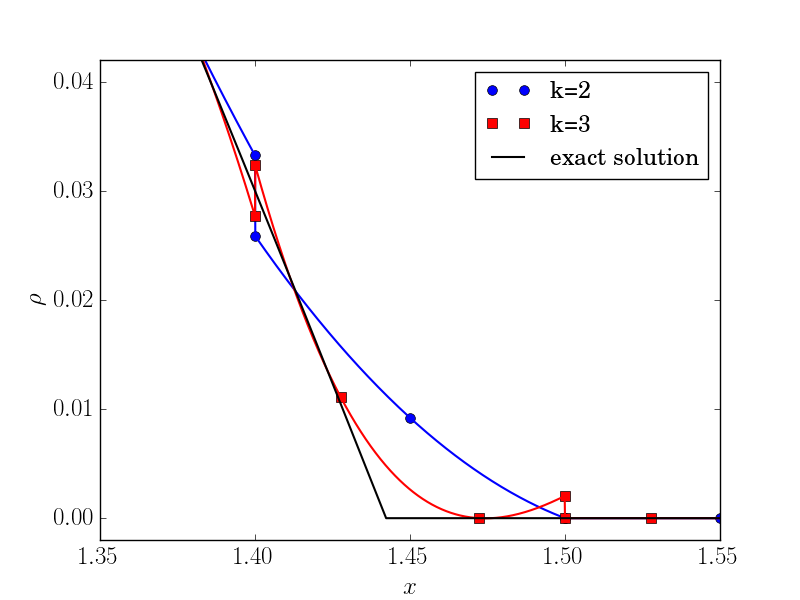
(b) Zoomed in figure near $x=3^{\frac{1}{3}}$.

Figure 4.1: Profiles of the numerical steady states for (4.2.1), with $\rho(x,0)=\max\{1-|x|,0\}$.

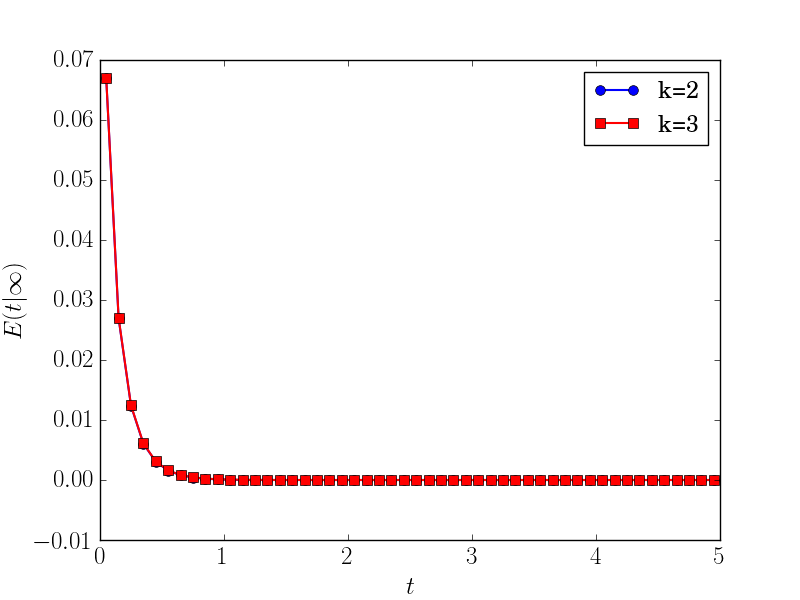
(a) $\rho(x,0)=\max\{1-|x|,0\}$.

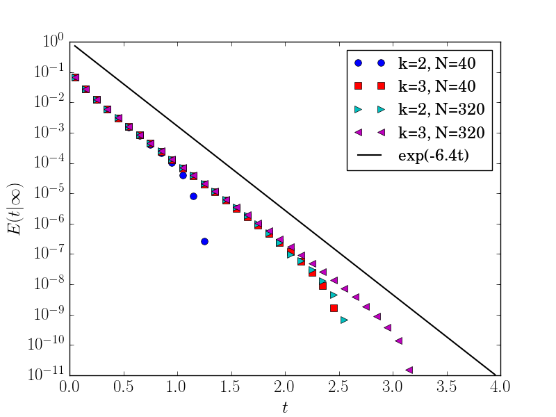
(b) $\rho(x,0)=\max\{1-|x|,0\}$.

Figure 4.2: The entropy and the relative entropy for (4.2.1), with $\rho(x,0)=\max\{1-|x|,0\}$.

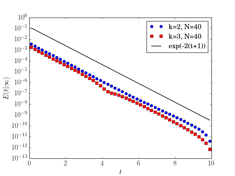
Figure 4.3: The relative entropy for porous equation, with $\rho(x,0)=\max\{1-|x-\frac{1}{2}|,0\}$.

For the symmetric initial condition, our numerical tests indicate the decay rates is around $e^{-6.7t}$. Indeed, symmetric initial data converge faster to equilibrium than the sharp rate since they preserve the invariance of the center mass, see [13] for more details. We then test the problem under the same settings, except for the initial condition shifted to the right $\rho(x,0)=\max\{1-|x-\frac{1}{2}|,0\}$ and the final time set to $t=10$. The corresponding plot of $E(t|\infty)$ is given in Figure 4.3 with the exponential decay rate $-2$, which coincides with the result in [19]. Similar numerical test can be found in [6].

Example 4.2.2 (Fokker-Planck equation).

In this numerical test, we consider the Fokker-Planck equation for modeling the relaxation of fermion and boson gases. The equation takes the form

$$\partial_{t}\rho=\partial_{x}\left(x\rho\left(1+\kappa\rho\right)+\partial_{x}\rho\right).$$

Here $\kappa=1$ corresponds to boson gases and $\kappa=-1$ relates to fermion gases. The long time asymptotics of the one dimensional model has been studied in [18] for $0\leq\rho\leq 1$. The authors point out the equation evolves to a steady state $\rho_{\infty}(x)=\frac{1}{\beta e^{\frac{x^{2}}{2}}-\kappa}$. The stationary solution minimizes the entropy functional

$$E=\int\left(\frac{|x|^{2}}{2}\rho+\rho\log(\rho)-\kappa(1+\kappa\rho)\log(1+\kappa\rho)\right)dx.$$

The relative entropy decays at an exponential rate $E(t|\infty)\leq E(0|\infty)e^{-2Ct}$, with $C=1$ for the boson case and $0<C<1$ for the fermion case. In our numerical test, we study the same entropy functional and set $f(\rho)=\rho(1+\kappa\rho)$, $H^{\prime}(\rho)=\log\left(\frac{\rho}{1+\kappa\rho}\right)$, $V=\frac{x^{2}}{2}$ in our numerical scheme. The limiter is turned on in the computation. The initial condition is chosen as $\rho(x,0)=\frac{1}{0.4\pi}e^{-\frac{(x-1)^{2}}{0.4}}$. We compute on the domain $[-10,10]$ with $100$ mesh cells, and march towards the steady state with $\tau=0.0002h^{2}$. The flux constant is set to $2$.

For both of the test cases, we use numerical steady states as references to calculate the relative entropy. The result for the boson case is given in Figure 4(a). As one can see, the decay rate is around $-2.6$. While for the fermion case, which is exhibited in Figure 4(b), the relative entropy decays at a slower rate of $-1.44$.

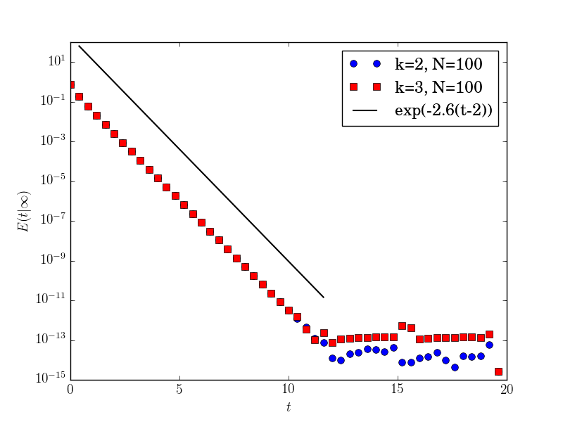
(a) Bose gas.

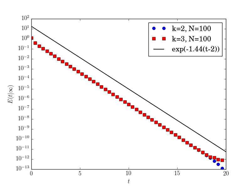
(b) Fermi gas.

Figure 4.4: Decay of the relative entropy for Fokker-Planck equation.

Example 4.2.3 (generalized Fokker-Planck equation for the boson gas).

Let us now consider the generalized Fokker-Planck equation with linear diffusion and superlinear drift

$$\partial_{t}\rho=\partial_{x}\left(x\rho(1+\rho^{N})+\partial_{x}\rho\right),$$

with $N$ being a positive constant. For $N>2$, it is reported in [1] that a critical mass phenomenon exists for one dimensional problems. An initial distribution with supercritical mass will evolve a singularity at the origin, which has been confirmed numerically in [6] and [37]. In this test, we repeat the numerical experiment in [6] and [37], setting

$$f(\rho)=\rho\left(1+\rho^{3}\right),H^{\prime}(\rho)=\log\frac{\rho}{\sqrt[3]{1+\rho^{3}}}\text{ and }V(x)=\frac{x^{2}}{2}.$$

The initial datum is chosen as

$$\rho(x,0)=\frac{M}{2\sqrt{2\pi}}\left(e^{-\frac{(x-2)^{2}}{2}}+e^{-\frac{(x+2)^{2}}{2}}\right).$$

We test with both the subcritical case with $M=1$ and the supercritical case with $M=10$. The $P^{4}$ elements are used in our numerical scheme and we compute on the domain $[-6,6]$ with $N=120$. For $M=1$, the time step is chosen as $\tau=0.003h^{2}$ and for $M=10$, it is $\tau=0.0005h^{2}$. And we use $g(\rho)=f(\rho)$ when defining the numerical flux. According to the numerical results in Figure 4.5, our scheme does capture the asymptotics of the equation.

(a) $M=1$.

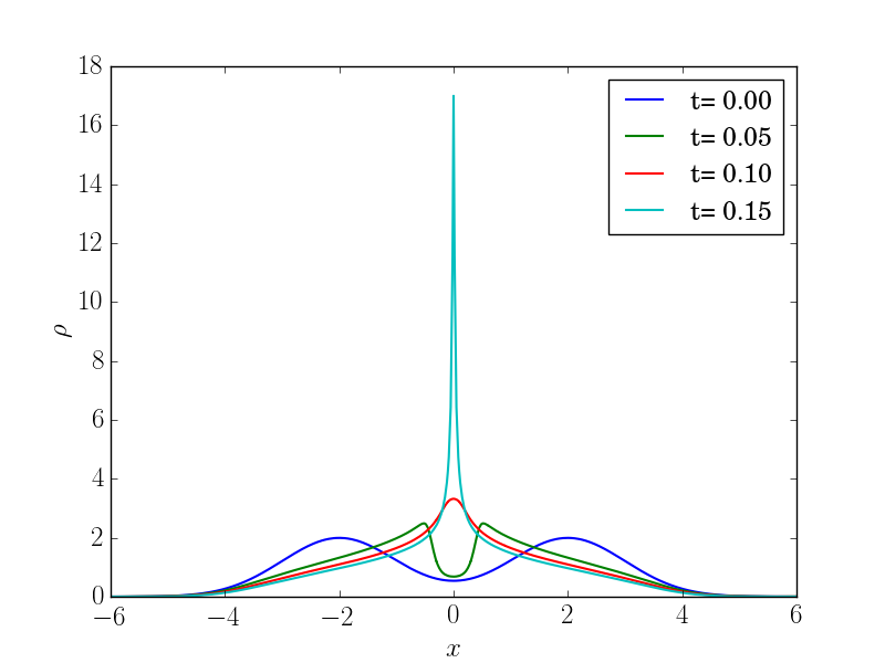
(b) $M=10$.

Figure 4.5: Evolution of $\rho$ of subcritical mass $M=1$ and supercritical mass $M=10$.

4.3 Aggregation models

Example 4.3.1 (nonlinear diffusion with smooth attraction kernel).

This numerical test is to study the dynamics of the equation with competing nonlinear diffusion and smooth nonlocal attraction,

$$\partial_{t}\rho=\partial_{x}\left(\rho\partial_{x}\left(\nu\rho^{m-1}+W\ast\rho\right)\right).$$

Here $0\leq\rho\leq 1$. $\nu>0$ and $m>1$ are parameters to be specified. The convolution kernel $W$ in this example is nonlocal and smooth. Under this setting, the attraction effect is weak and the solution would either end up with a steady state or spread out in the whole domain with bounded initial data. The compactly supported steady state is of special interest, due to its application for modeling the biological aggregation, such as flocks and swarms. Indeed, such stationary solution can be reached for $m>2$ with arbitrary $\nu$. While for $1<m\leq 2$, the long time behavior of the solution can be sophisticated. We refer to [9] and [10] for details. For our numerical test, we focus on the specific setting,

$$\left\{\begin{aligned} \partial_{t}\rho&=\partial_{x}(\rho\partial_{x}(\nu\rho^{m-1}+W\ast\rho)),W(x)=-\frac{1}{\sqrt{2\pi}}e^{-\frac{x^{2}}{2}},x\in[-6,6],\\ \rho(x,0)&=\frac{1}{2\sqrt{2\pi}}\left(e^{-\frac{(x-\frac{5}{2})^{2}}{2}}+e^{-\frac{(x+\frac{5}{2})^{2}}{2}}\right).\end{aligned}\right.$$

We apply periodic boundary conditions and use a mesh with $N=120$ for computation. The $P^{2}$ scheme is used for the numerical test, and the time step is chosen as $\tau=0.05h^{2}$. In Figure 4.6, we depict the numerical solution at $T=1800$ with $m=1.5$, $\nu=0.33$, $m=2$, $\nu=0.48$ and $m=3$, $\nu=1.48$, which are used as the reference steady states when evaluating the relative entropy.

According to the plot, one can see that a larger $m$ corresponds to a steady state with a sharper transition along the boundary of the support. Indeed, one should expect the Hölder continuity with the exponent $\alpha=\min\{1,1/(m-1)\}$.

Figure 4.6: Solution profile at $T=1800$.

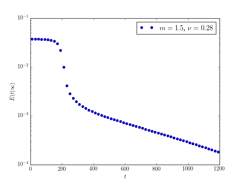
(a) Relative entropy.

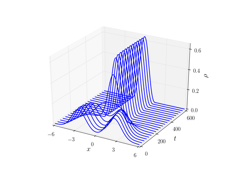
(b) Evolution.

Figure 4.7: $m=1.5$, $\nu=0.28.$

We track the solution profile and the relative entropy. For $m=1.5$, as one can see from Figure 7(a), the dynamics of the problem distinguishes from the test cases for Fokker-Planck type equations. The relative entropy decays slowly at first, then it follows with a steep drop at a certain time. After that, the relative entropy decays exponentially. The behavior can be explained with Figure 7(b). At the beginning, the two bumps of the initial condition stay away from each other, their interaction is weak hence the equation evolves at a slow rate. When they get closer, the attraction becomes strong. A sudden decay of the relative entropy occurs when the two bumps merge. After that, the contribution of the interaction potential to the total energy becomes small. The equation is again dominated by the diffusion term, and the relative entropy decays exponentially as we have seen before.

We omit the plots for $m=2$. And for $m=3$, the diffusion is relatively weak and the exponential decay after the steep drop is hard to observe. Hence we only plot the entropy in the normal scale. But still we can see the sharp drop when the bumps merge in Figure 4.8.

The initial stage featured with the weak long-range-interaction is referred as metastability. If multiple bumps exist, the relative entropy can decay in a staircase fashion. For example, we test the problem with $m=6$, $\nu=6$ and $\rho(x,0)=\frac{3}{20}\max\{1-|x-\frac{19}{4}|,0\}+\frac{1}{4}\max\{1-|x-2|,0\}+\frac{1}{5}\max\{1-|x+\frac{17}{40}|,0\}+\frac{2}{5}\max\{1-|x+\frac{15}{4}|,0\}$. The relative entropy and dynamics are given in Figure 4.9.

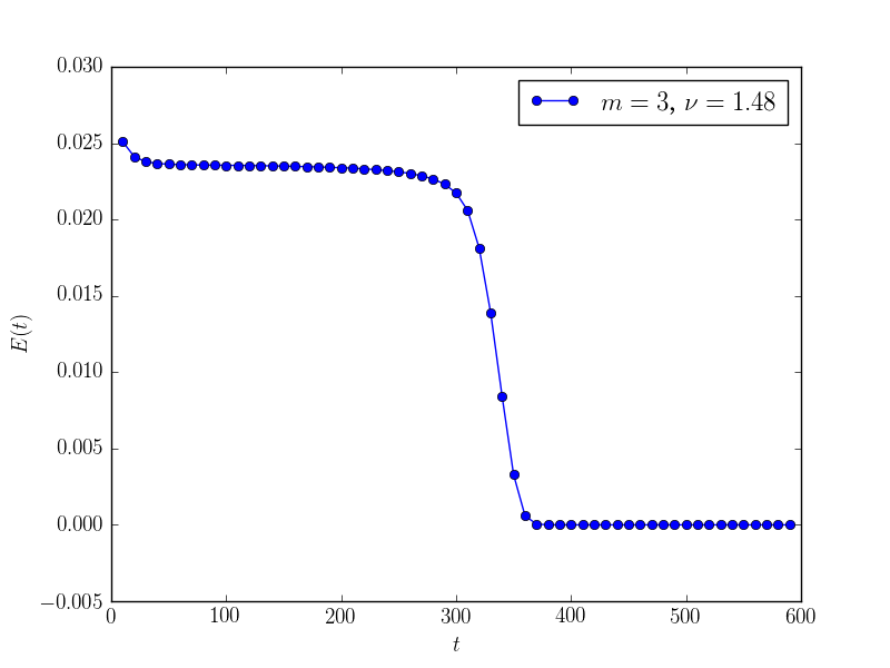
(a) Entropy.

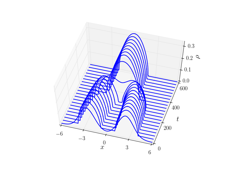
(b) Evolution.

Figure 4.8: $m=3$, $\nu=1.48$.

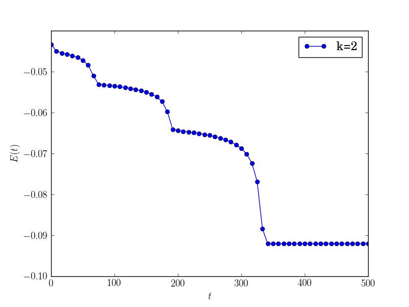
(a) Entropy.

(b) Evolution.

Figure 4.9: Stepwise decay: $m=6$, $\nu=6$.

Example 4.3.2 (nonlinear diffusion with compactly supported attraction kernel).

In the previous test, the attraction effect is global and the steady state will be connected for one dimensional problems. But when $W$ is local, the connectivity of the equilibrium can be affected by the initial mass distribution. Let us consider the following problem

$$\left\{\begin{aligned} \partial_{t}\rho&=\partial_{x}\left(\rho\partial_{x}\left(\frac{1}{4}\rho^{2}+W\ast\rho\right)\right),\quad W=-\max\{1-|x|,0\},\quad x\in[-4,4],\\ \rho(x,0)&=\chi_{[-a,a]}(x),\end{aligned}\right.$$ (4.3)

with periodic boundary conditions. We compute with $k=2$ with the number of cells $N=80$.

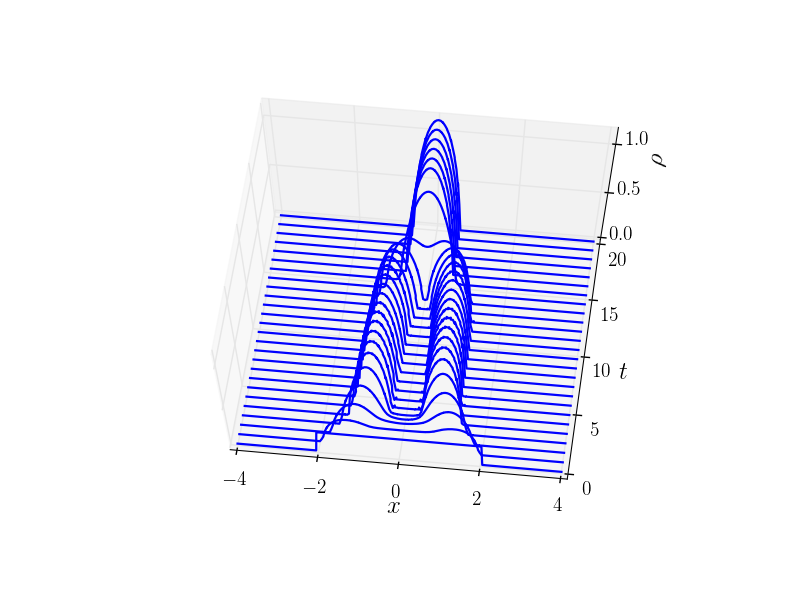
(a) $\rho(x,0)=\chi_{[-2,2]}(x)$

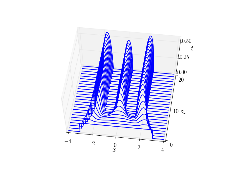
(b) $\rho(x,0)=\chi_{[-3,3]}(x)$

Figure 4.10: Evolution of (4.3) with different initial conditions.

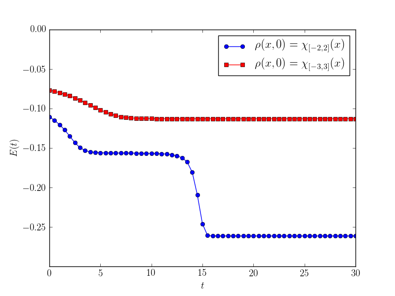
(a) Entropy

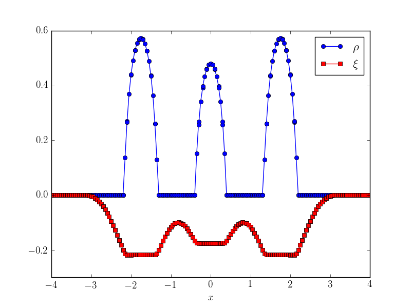
(b) $\xi$ and $\rho$ at $t=30$ for $\rho(x,0)=\chi_{[-3,3]}(x)$

Figure 4.11: Entropy and the steady state of (4.3).

To convince the readers that the disconnected profile in Figure 10(b) is indeed the stationary solution, we plot $\rho$ and $\xi$ in Figure 11(b). As one can observe, $\rho\partial_{x}\xi\approx 0$. Hence $\partial_{t}\rho\approx 0$ and $\rho$ will be trapped in this steady state. Therefore, the observation in Figure 4.10 confirms our previous claim, that different initial density distributions may end up with steady states with distinct connectivity. Let us remark that such phenomenon has also been explored numerically in [12].

5 Two dimensional numerical tests

Example 5.1 (accuracy test).

We consider the initial value problem with a source term,

$$\left\{\begin{aligned} \partial_{t}\rho&=\nabla\cdot\left(\rho\nabla\left(\log(\rho)+\sin(x+y)+W\ast\rho\right)\right)+F,(x,y)\in(-\pi,\pi)\times(-\pi,\pi),t>0\\ W(x,y)&=\cos(x+y),\\ F(x,y)&=4\sin(x+y)+\cos(x+y+t)+\left(2+8\pi^{2}\right)\sin(x+y+t)\\ &-2\cos\left(2(x+y)+t\right)-4\pi^{2}\cos\left(2\left(x+y+t\right)\right)\\ \rho(x,y,0)&=\sin(x+y)+2.\\ \end{aligned}\right.$$ (5.1)

Here periodic boundary conditions are applied and $W\ast\rho=\int_{-\pi}^{\pi}\int_{-\pi}^{\pi}W(x-\tilde{x},y-\tilde{y})\rho(\tilde{x},\tilde{y})d\tilde{x}d\tilde{y}$. One can check that the exact solution to (5.1) is $\rho(x,y,t)=2+\sin(x+y+t)$. We use the time step $\tau=0.0005(h^{x})^{2}$ for the calculation. The error table is given in Table 5.1.

k	N	$L^{1}$ error	order	$L^{2}$ error	order	$L^{\infty}$ error	order
1	$10\times 10$	5.11679	-	1.02912	-	0.400769	-
	$20\times 20$	1.15240	2.15	0.231872	2.15	0.944210E-01	2.09
	$40\times 40$	0.301086	1.94	0.621649E-01	1.90	0.241975E-01	1.96
2	$10\times 10$	1.45276	-	0.306948	-	0.167537	-
	$20\times 20$	0.222326	2.71	0.431470E-01	2.83	0.297235E-01	2.49
	$40\times 40$	0.356271E-01	2.64	0.720268E-02	2.58	0.513506E-02	2.53
3	$10\times 10$	0.377751E-01	-	0.792888E-02	-	0.439644E-02	-
	$20\times 20$	0.229221E-02	4.04	0.525495E-03	3.92	0.294146E-03	3.90
	$40\times 40$	0.137322E-03	4.06	0.333325E-04	3.98	0.205418E-04	3.83
4	$10\times 10$	0.224001E-02	-	0.511292E-03	-	0.294120E-03	-
	$20\times 20$	0.676477E-04	5.05	0.143874E-04	5.15	0.115235E-04	4.67
	$40\times 40$	0.243927E-05	4.80	0.524241E-06	4.78	0.450331E-06	4.68

Table 5.1: Two dimensional accuracy test, with smooth data and periodic boundary conditions.

Example 5.2 (dumbbell model for polymers).

The dumbbell model is widely used to describe the rheological behavior of dilute polymer solutions. In this model, the polymer molecular is treated as a dumbbell made of two beads jointed by a spring. We will consider the simplest case, in which the flow is homogeneous and the scaling constant is set to $1$. Then the configuration probability density is governed by the Fokker-Plank equation,

$$\partial_{t}\rho(\mathbf{x},t)=\nabla\cdot(\rho\nabla(U-\frac{1}{2}\mathbf{x}K\mathbf{x}))+\Delta\rho.$$ (5.2)

Here $\mathbf{x}=(x,y)$ corresponds to the direction vector of the molecule, while $U$ is the spring potential and the $2\times 2$ matrix $K$ is the velocity gradient of the background flow. For the incompressible flow, $\text{Tr}(K)=0$. In our numerical test, we consider the finitely extensible nonlinear elastic (FENE) model. The potential $U$ is given by

$$U(\mathbf{x})=-\frac{r^{2}}{2}\log\left(1-\frac{|\mathbf{x}|^{2}}{r^{2}}\right).$$ (5.3)

It is close to the Hookean potential when $|\mathbf{x}|\ll r$, while the distance between the two beads are restricted within $r$. Rigorously, one should consider the equation on the ball $\{\mathbf{x}:|\mathbf{x}|\leq r\}$, and the singularity near the boundary will cause challenges both analytically and numerically, see [30, 36, 41, 39] and the references therein. While in our numerical test, we only consider a simpler case, that the solution seems to be supported within the ball and it hardly reaches the boundaries. More specifically, we solve (5.2)-(5.3) with $r=5$ and $K=\left(\begin{matrix}0.3&0.2\\ 0.2&-0.3\end{matrix}\right)$. The initial condition is set as

$$\begin{split}\rho(x,y,0)=&c\max\{24-(x^{2}+y^{2}),0\}\\ &\left(e^{-\frac{(x-2)^{2}+(y-2)^{2}}{2\sigma^{2}}}+e^{-\frac{(x+2)^{2}+(y+2)^{2}}{2\sigma^{2}}}+e^{-\frac{(x-1)^{2}+(y-1)^{2}}{2\sigma^{2}}}+e^{-\frac{(x+1)^{2}+(y+1)^{2}}{2\sigma^{2}}}\right),\end{split}$$ (5.4)

where $\sigma^{2}=0.2$ and $c$ the normalization constant. We use the $P^{3}$ DG scheme on a $[-5,5]\times[-5,5]$ domain with $50\times 50$ mesh cells. The time step is chosen as $\tau=2\times 10^{-6}$. In Figure 5.1, we plot the evolution from $T=0$ to $T=0.6$. It seems the numerical solution merges to a single peak.

(a) $t=0$.

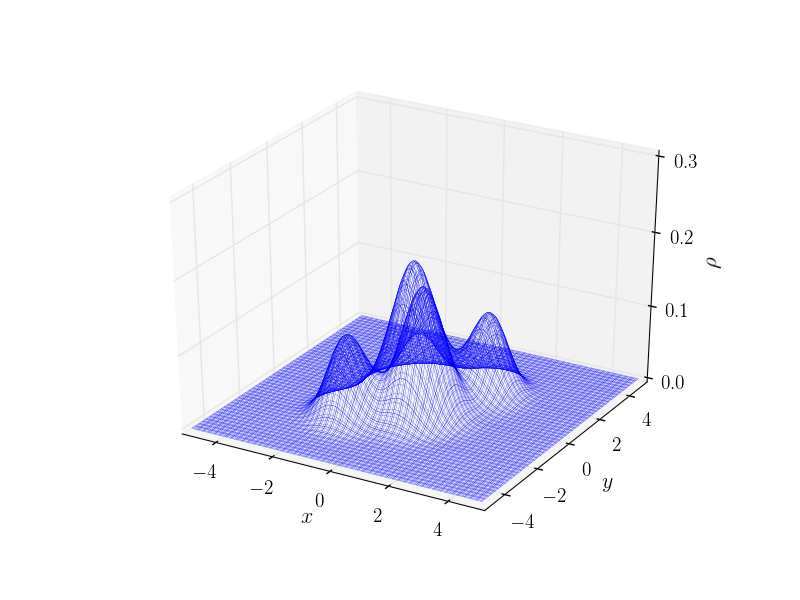
(b) $t=0.2$.

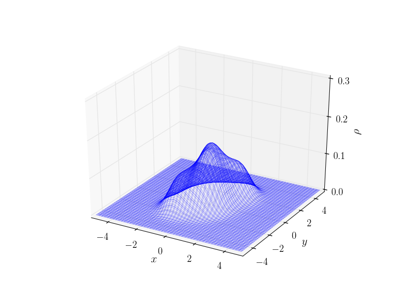
(c) $t=0.4$.

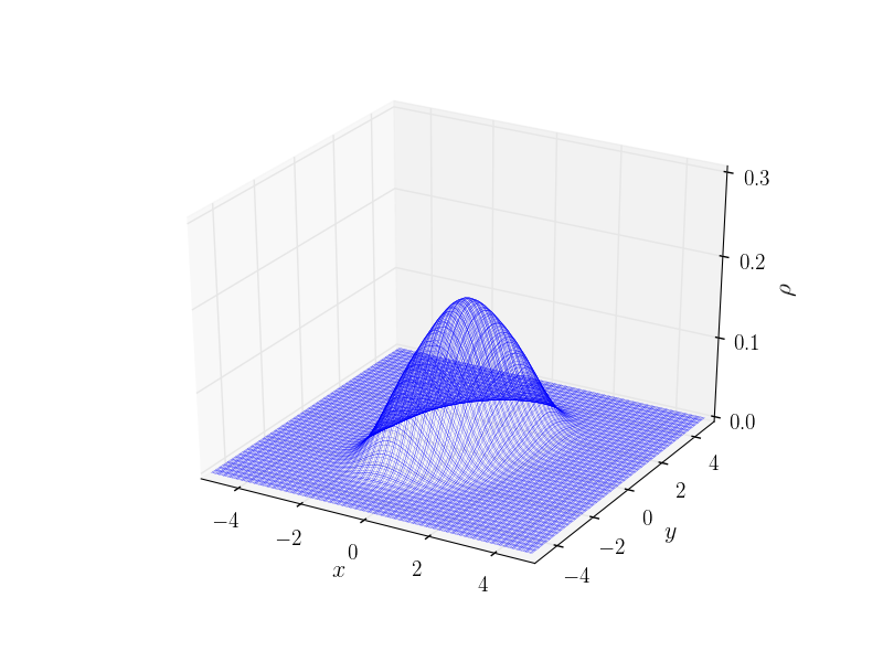
(d) $t=0.6$.

Figure 5.1: Evolution of the dumbbell model (5.2) with the FENE potential (5.3).

Example 5.3 (Patlak-Keller-Segel system for chemotaxis).

Chemotaxis is defined as a move of an organism along a chemical concentration gradient. Bacteria can produce this chemo-attractant themselves, creating thus a long range nonlocal interaction between them. The Patlak-Keller-Segel system is a mathematical model to describe the motion of the organism. Its simplified version is given by

$$\left\{\begin{aligned} \partial_{t}\rho&=\Delta\rho-\nabla\cdot(\rho\nabla c),\qquad(x,y)\in\mathbb{R}^{2},t>0,\\ -\Delta c&=\rho,\qquad(x,y)\in\mathbb{R}^{2},t>0,\\ \rho(x,y,0)&=\rho_{0}(x,y).\end{aligned}\right.$$

The equation can be rewritten in a compact way

$$\partial_{t}\rho=\nabla\cdot\left(\rho\nabla\left(\log(\rho)+W\ast\rho\right)\right),\quad W(x,y)=\frac{1}{2\pi}\log(\sqrt{x^{2}+y^{2}})\quad(x,y)\in\mathbb{R}^{2},t>0.$$ (5.5)

Such system has been studied intensively in the past decades. It has been shown that the behavior of the equation (5.5) is determined by its initial mass (see [7], for example). If the initial value $M$ is smaller than a critical value $M_{c}=8\pi$, then the solution will exist globally. Otherwise, if $M$ lies beyond $M_{c}$, the solution will blow up in a finite time, which is referred as chemotactic collapse.

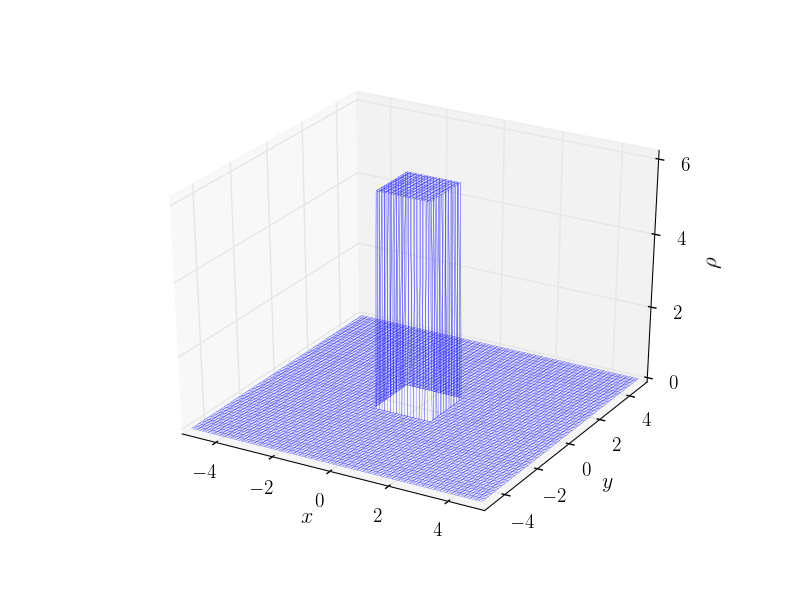
(a) $t=0$.

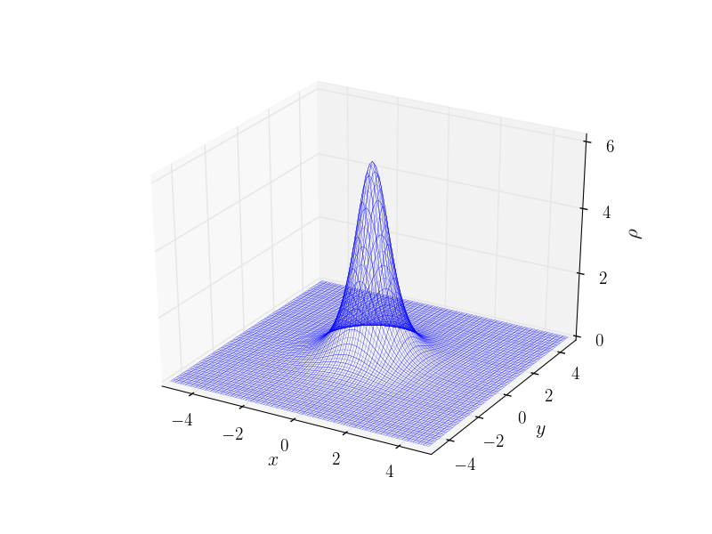
(b) $t=4$.

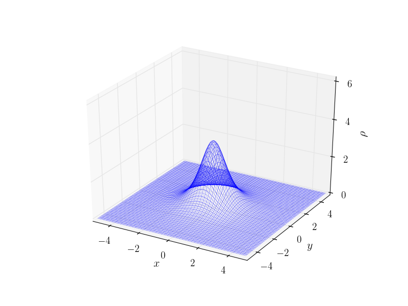
(c) $t=8$.

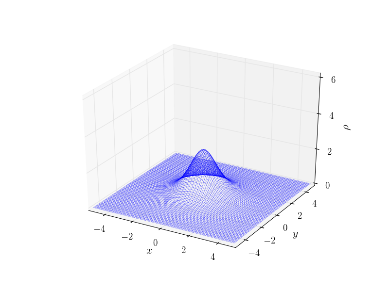
(d) $t=12$.

(e) $t=16$.

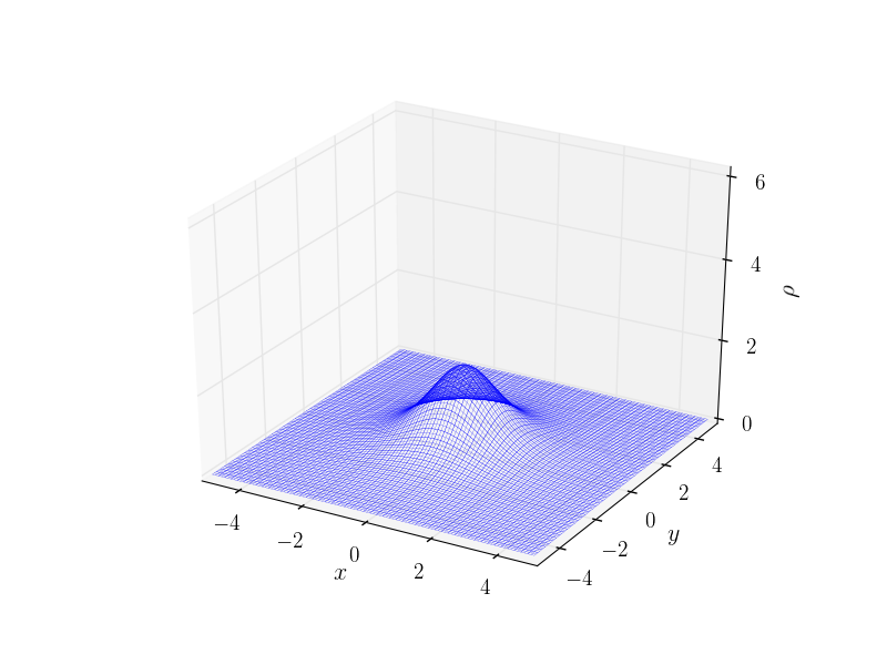
(f) $t=20$.

Figure 5.2: Evolution of Patlak-Keller-Segel equation (5.5) with subcritical mass.

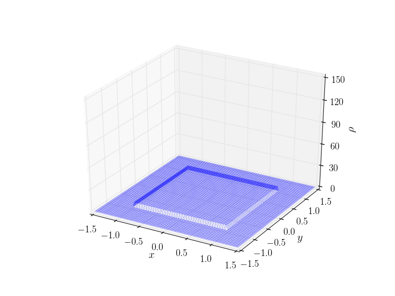
(a) $t=0$.

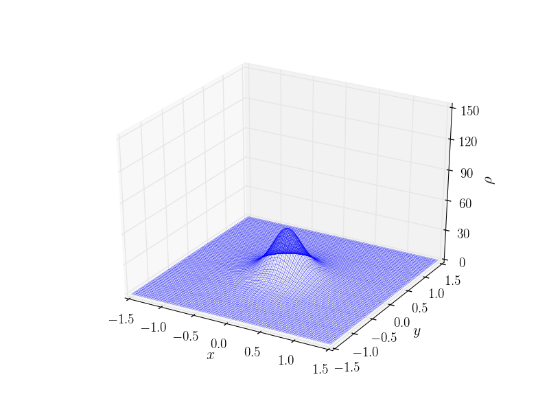
(b) $t=0.5$.

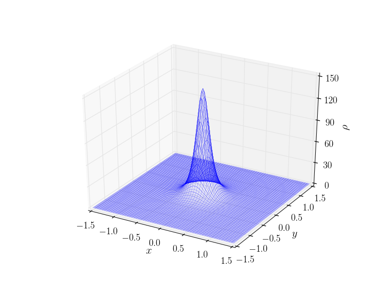
(c) $t=1$.

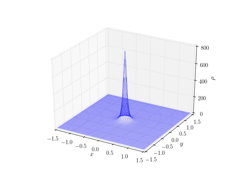
(d) $t=1.5$.

(e) $t=2$.

Figure 5.3: Evolution of Patlak-Keller-Segel equation (5.5) with supercritical mass.

In our numerical test, we consider both the subcritical case $\rho_{0}(x)=2(\pi-0.2)1_{[-1,1]\times[-1,1]}(x,y)$ and the super-critical case $\rho_{0}(x)=2(\pi+0.2)1_{[-1,1]\times[-1,1]}(x,y)$. The computational domain is set as $[-5,5]\times[-5,5]$ and $[-\frac{3}{2},\frac{3}{2}]\times[-\frac{3}{2},\frac{3}{2}]$ respectively. We use the $P^{2}$ scheme for computation and $N_{x}=N_{y}=50$. The time step is set as $\tau=0.0005(h^{x})^{2}$. The plots are given in Figure 5.2 and Figure 5.3. As one can see, the numerical solution dissipates for $\rho_{0}(x)=2(\pi-0.2)1_{[-1,1]\times[-1,1]}(x,y)$ and it evolves to a spike centered at the origin for $\rho_{0}(x)=2(\pi+0.2)1_{[-1,1]\times[-1,1]}(x,y)$.

6 Concluding remarks

In this paper, we develop a high order DG method for solving a class of parabolic equations and gradient flow problems with interaction potentials. Such equations are governed by an entropy-entropy dissipation relationship and are featured with non-negative solutions. By applying the Gauss-Lobatto quadrature rule, our numerical scheme admits an entropy inequality for problems with smooth interaction kernels. Furthermore, with the SSP-RK time discretization and the positivity-preserving limiter, the fully discretized scheme preserves the non-negativity of the numerical density. It also conserves mass, and preserves numerical steady states for certain problems. We also apply the method to two dimensional problems on Cartesian meshes. Numerical examples are given to demonstrate the performance of the scheme.

References

- [1] N.B. Abdallah, I.M. Gamba and G. Toscani. On the minimization problem of sub-linear convex functionals. Kinetic and Related Models, 4(4):857–871, 2011.
- [2] L. Ambrosio, N. Gigli and G. Savaré. Gradient Flows: In Metric Spaces and in the Space of Probability Measures. Springer Science & Business Media, 2008.
- [3] F. Bassi and S. Rebay. A high-order accurate discontinuous finite element method for the numerical solution of the compressible Navier-Stokes equations. Journal of Computational Physics, 131:267–279, 1997.
- [4] D. Benedetto, E. Caglioti and M. Pulvirenti. A kinetic equation for granular media. RAIRO-Modélisation Mathématique et Analyse Numérique, 31(5):615–641, 1997.
- [5] D. Benedetto, E. Caglioti, J. A. Carrillo, and M. Pulvirenti. A non-Maxwellian steady distribution for one-dimensional granular media. J. Statist. Phys., 91:979–990, 1998.
- [6] M. Bessemoulin-Chatard and F. Filbet. A finite volume scheme for nonlinear degenerate parabolic equations. SIAM Journal on Scientific Computing, 34(5):B559–B583, 2012.
- [7] A. Blanchet, J. Dolbeault and B. Perthame. Two-dimensional Keller-Segel model: optimal critical mass and qualitative properties of the solutions. Electronic Journal of Differential Equations, 44:32pp, 2006.
- [8] M. Burger, J.A. Carrillo and M.T. Wolfram. A mixed finite element method for nonlinear diffusion equations. Kinetic and Related Models, 3(1):59–83, 2010.
- [9] M. Burger, R. Fetecau and Y. Huang. Stationary states and asymptotic behavior of aggregation models with nonlinear local repulsion. SIAM Journal on Applied Dynamical Systems, 13(1):397–424, 2014.
- [10] M. Burger, M. Di Francesco, and M. Franek. Stationary states of quadratic diffusion equations with long-range attraction. Communications in Mathematical Sciences, 11(3):709–738, 2013.
- [11] M.H. Carpenter, T.C. Fisher, E.J. Nielsen and S.H. Frankel. Entropy stable spectral collocation schemes for the Navier-Stokes equations: discontinuous interfaces. SIAM Journal on Scientific Computing, 36:B835–B867, 2014.
- [12] J.A. Carrillo, A. Chertock and Y. Huang. A finite-volume method for nonlinear nonlocal equations with a gradient flow structure. Communications in Computational Physics, 17(1):233–258, 2015.
- [13] J. A. Carrillo, M. Di Francesco, and G. Toscani. Strict contractivity of the 2-Wasserstein distance for the porous medium equation by mass-centering. Proc. Amer. Math. Soc., 135:353–363, 2007.
- [14] J.A. Carrillo, Y. Huang, F.S. Patacchini and G. Wolansky. Numerical study of a particle method for gradient flows. Kinetic and Related Models, 10(3):613–641, 2017.
- [15] J.A. Carrillo, A. Jüngel, P.A. Markowich, G. Toscani and A. Unterreiter. Entropy dissipation methods for degenerate parabolic problems and generalized Sobolev inequalities. Monatshefte für Mathematik, 133(1):1–82, 2001.
- [16] J.A. Carrillo, R.J. McCann and C. Villani. Kinetic equilibration rates for granular media and related equations: entropy dissipation and mass transportation estimates. Revista Matematica Iberoamericana, 19(3):971–1018, 2003.
- [17] J.A. Carrillo, H. Ranetbauer and M.T. Wolfram. Numerical simulation of nonlinear continuity equations by evolving diffeomorphisms. Journal of Computational Physics, 327:186–202, 2016.
- [18] J.A. Carrillo, J. Rosado and F. Salvarani. 1D nonlinear Fokker-Planck equations for fermions and bosons. Applied Mathematics Letters, 21(2):148–154, 2008.
- [19] J.A. Carrillo and G. Toscani. Asymptotic L1-decay of solutions of the porous medium equation to self-similarity. Indiana University Mathematics Journal, 49(1):113–142, 2000.
- [20] T. Chen and C.-W. Shu. Entropy stable high order discontinuous Galerkin methods with suitable quadrature rules for hyperbolic conservation laws. Journal of Computational Physics, in revision.
- [21] Y. Cheng and C.-W. Shu. A discontinuous Galerkin finite element method for time dependent partial differential equations with higher order derivatives. Mathematics of computation, 77(262):699–730, 2008.
- [22] K. Craig and A. Bertozzi. A blob method for the aggregation equation. Mathematics of Computation, 85(300):1681–1717, 2016.
- [23] B. Cockburn, S. Hou, and C.-W. Shu. The Runge-Kutta local projection discontinuous Galerkin finite element method for conservation laws IV: the multidimensional case. Mathematics of Computation, 54:545–581, 1990.
- [24] B. Cockburn, S.-Y. Lin, and C.-W. Shu. TVB Runge-Kutta local projection discontinuous Galerkin finite element method for conservation laws III: one-dimensional systems. Journal of Computational Physics, 84:90–113, 1989.
- [25] B. Cockburn and C.-W. Shu. TVB Runge-Kutta local projection discontinuous Galerkin finite element method for conservation laws II: general framework. Mathematics of computation, 52:411–435, 1989.
- [26] B. Cockburn and C.-W. Shu. The Runge-Kutta local projection -discontinuous-Galerkin finite element method for scalar conservation laws. RAIRO-Modélisation Mathématique et Analyse Numérique, 25:337–361, 1991.
- [27] B. Cockburn and C.-W. Shu. The Runge-Kutta discontinuous Galerkin method for conservation laws V: multidimensional systems. Journal of Computational Physics, 141:199–224, 1998.
- [28] B. Cockburn and C.-W. Shu. The local discontinuous Galerkin method for time-dependent convection-diffusion systems. SIAM Journal on Numerical Analysis, 35(6):2440–2463, 1998.
- [29] B. Cockburn and C.-W. Shu. Runge-Kutta discontinuous Galerkin methods for convection-dominated problems. Journal of Scientific Computing, 16(3):172–261, 2001.
- [30] Q. Du, C. Liu and P. Yu. FENE dumbbell model and its several linear and nonlinear closure approximations. Multiscale Modeling & Simulation, 4(3):709–731, 2005.
- [31] G.J. Gassner. A skew-symmetric discontinuous Galerkin spectral element discretization and its relation to SBP-SAT finite difference methods. SIAM Journal on Scientific Computing, 35:A1233–A1253, 2013.
- [32] G.J. Gassner, A.R. Winters and D.A. Kopriva. A well balanced and entropy conservative discontinuous Galerkin spectral element method for the shallow water equations. Applied Mathematics and Computation, 272:291–308, 2016.
- [33] S. Gottlieb, C.-W. Shu and E. Tadmor. Strong stability-preserving high-order time discretization methods. SIAM Review, 43(1):89–112, 2001.
- [34] J.S. Hesthaven, S. Gottlieb and D. Gottlieb. Spectral Methods for Time-dependent Problems. Cambridge University Press, 2007.
- [35] J.S. Hesthaven and T. Warburton. Nodal Discontinuous Galerkin Methods: Algorithms, Analysis, and Applications. Springer Science & Business Media, 2007.
- [36] C. Liu and H. Liu. Boundary conditions for the microscopic FENE models. SIAM Journal on Applied Mathematics, 68(5):1304-1315, 2008.
- [37] H. Liu and Z. Wang. An entropy satisfying discontinuous Galerkin method for nonlinear Fokker-Planck equations. Journal of Scientific Computing, 68(3):1217–1240, 2016.
- [38] H. Liu and J. Yan. The direct discontinuous Galerkin (DDG) methods for diffusion problems. SIAM Journal on Numerical Analysis, 47(1):675–698, 2009.
- [39] H. Liu and H. Yu. Maximum-principle-satisfying third order discontinuous Galerkin schemes for Fokker-Planck equations. SIAM Journal on Scientific Computing, 36(5):A2296–A2325, 2014.
- [40] A. Mogilner and L. Edelstein-Keshet. A non-local model for a swarm. Journal of Mathematical Biology, 38(6):534–570, 1999.
- [41] J. Shen and H. Yu. On the approximation of the Fokker-Planck equation of the finitely extensible nonlinear elastic dumbbell model I: a new weighted formulation and an optimal spectral-Galerkin algorithm in two dimensions. SIAM Journal on Numerical Analysis, 50(3):1136–1161, 2012.
- [42] C.M. Topaz, A.L. Bertozzi and M.A. Lewis. A nonlocal continuum model for biological aggregation. Bulletin of Mathematical Biology, 68(7):1601, 2006.
- [43] C. Villani. Topics in Optimal Transportation. American Mathematical Society, 2003
- [44] X. Zhang. On positivity-preserving high order discontinuous Galerkin schemes for compressible Navier-Stokes equations. Journal of Computational Physics, 328:301–343, 2017.
- [45] X. Zhang and C.-W. Shu. On maximum-principle-satisfying high order schemes for scalar conservation laws. Journal of Computational Physics, 229(9):3091–3120, 2010.
- [46] X. Zhang and C.-W. Shu. Maximum-principle-satisfying and positivity-preserving high-order schemes for conservation laws: survey and new developments. Proceedings of the Royal Society of London A: Mathematical, Physical and Engineering Sciences, 467(2134):2752–2776, 2011.