Dept. Mathematical and Computer Sciences, Physical and Earth Sciences,
University of Messina, Viale F. Stagno d’Alcontres 31, I-98166 Messina, Italy e-mail: imbesim@unime.it, monicalb@unime.it, snapmode91@gmail.com

Abstract: In this paper algebraic and combinatorial properties and a computation of the number of the spanning trees are developed for Jahangir graphs.

AMS 2010 Subject Classification: Primary 68R10; Secondary 05C05; 05C85
Key words and phrases: Connected graphs; Cyclic graphs; Spanning trees.

Introduction

Let $\mathcal{G}$ be a finite simple connected cyclic graph having vertex set $V(\mathcal{G})$ and edge set $E(\mathcal{G})$. We refer to [14] for a detailed presentation of classical algebraic topics about graph theory. In [7, 5, 6, 8, 9] interesting results about algebraic and combinatorial properties linked to finite graphs can be found.
A spanning tree of $\mathcal{G}$ is an acyclic connected subgraph of $\mathcal{G}$ that contains all the vertices of $\mathcal{G}$. Let’s denote by $s(\mathcal{G})$ the collection of all edge-sets of the spanning trees of $\mathcal{G}$.
An effective analytical method for obtaining systematically all the existing spanning trees of $\mathcal{G}$ is the so-called cutting-down method: it consists of removing an appropriate number of edges from the graph for making it acyclic.
This work is devoted in studying an alternative method for the computation of the spanning trees of simple connected cyclic graphs, including for instance those considered in [1, 2, 10]. Specifically, combinatorial properties of the spanning trees of the remarkable class of Jahangir graphs, defined in [12], will be discussed and an algorithmic method to determine how many and what are the spanning trees of such type of graphs will be developed. This provides a general procedure for the calculation of the number $\sigma$ of their spanning trees.
The paper is structured as follows.
In section 1, we introduce fundamental notions on graphs theory like simple, connected, cyclic graphs, incidence and adjacency matrices and the Laplacian matrix associated to a graph, see also [4]; moreover, it is proved an important theorem, the Matrix Tree Theorem, due to G. Kirchhoff, for determining the total number of the spanning trees of any graph. Such a theorem uses the calculation of the eigenvalues of the associated Laplacian matrix ([3, 13]).
In section 2, Jahangir graphs $J_{n,m}$ are analyzed and their symmetric properties highlighted; their shape was inspired by a drawing carved in the mausoleum of the Indian Grand Mogul Jahangir (1569-1627) located in Lahore, Pakistan. The theoretical issue is focused in finding the number of the spanning trees for simple connected cycled graphs using a method independent of the spectrum of the associated Laplacian matrix. Therefore it provides an alternative process to compute how many and which are the spanning trees of such graphs.
The original algorithm and the source code for determining the collection of all edge-sets of the spanning trees for Jahangir graphs $J_{n,m}$ are displayed; it is possible to extend them to any simple connected cyclic graph.
Moreover, an application of sensitive data transmission arising from security real problems is illustrated.
In section 3, interesting relationships on the number of spanning trees of Jahangir graphs $J_{n,m}$ with same $n$ or same $m$ are considered, for more precision we conjecture that the fraction between the number of spanning trees related to Jahangir graphs having same first indices $n$ and consecutive second indices $m$ tends to a constant, distinct for each choice of $n$.

1 Preliminary notions and classical methods

Here we give some basic definitions and notations which will be used throughout the paper.
A (finite) graph $\mathcal{G}$ is an ordered triple $(V(\mathcal{G}),E(\mathcal{G}),f)$ such that $V(\mathcal{G})=\{v_{1},\ldots,v_{n}\}$ is the set of the vertices of $\mathcal{G}$, $E(\mathcal{G})=\{\{v_{i},v_{j}\}\ |\ v_{i},v_{j}\in V(\mathcal{G})\}$ the set of edges of $\mathcal{G}$ and $f:E(\mathcal{G})\longrightarrow V(\mathcal{G})\times V(\mathcal{G})$ the incidence function.
$\mathcal{G}$ is said to be simple if, for all $\{v_{i},v_{j}\}\in E(\mathcal{G})$, it is $v_{i}\neq v_{j}\,$.
A subgraph of $\mathcal{G}$ is a graph with all of its vertices and edges belonging to $\mathcal{G}$.
A spanning subgraph of $\mathcal{G}$ is a subgraph containing all the vertices of $\mathcal{G}$.
A graph which has no isolated subgraphs is called connected.
The degree of a vertex $v$ of $\mathcal{G}$ consists of the number of edges that converge in $v$ .
A walk of $\mathcal{G}$ of length $q$ is an alternating sequence of $q\!+\!1$ vertices and $q$ edges beginning and ending with vertices in which each edge is incident with the two vertices immediately preceding and following it. A path of $\mathcal{G}$ is a walk having all the vertices, and thus all the edges, distinct.
A walk of $\mathcal{G}$ is said to be closed if the exterior vertices coincide.
A closed path of $\mathcal{G}$ of length $q\geq 3$ is called cycle; in particular, it is a subgraph $C_{q}$ such that $E(C_{q})=\big{\{}\{v_{i_{1}},v_{i_{2}}\},\{v_{i_{2}},v_{i_{3}}\},\ldots,$ $\{v_{i_{q-1}},v_{i_{q}}\},\{v_{i_{q}},v_{i_{1}}\}\big{\}}$, where $\{v_{i_{1}},\ldots,v_{i_{q}}\}\in V(\mathcal{G})$ and $v_{i_{j}}\neq v_{i_{k}}$ if $i_{j}\neq i_{k}$.
A graph which has no cycles is called acyclic.
A tree is a connected acyclic graph. Any graph without cycles is a forest, thus the connected subgraphs of a forest are trees.

Definition 1.1.

A spanning tree of a simple connected finite graph $\mathcal{G}$ is a subtree of $\mathcal{G}$ that contains every vertex of $\mathcal{G}$.
We denote by $s(\mathcal{G})$ the collection of all edge-sets of the spanning trees of $\mathcal{G}$:

$$s(\mathcal{G})=\{E(G_{i})\subset E(\mathcal{G}),\textrm{where}\ T_{i}\ \textrm{is a spanning tree of}\ \mathcal{G}\}.$$

It is well-known that, for any simple finite connected graph, spanning trees always exist. One can systematically find a spanning tree by using the cutting-down method, which says that a spanning tree of a simple finite connected graph can be obtained by removing one edge from each cycle appearing in the graph.
We denote by $\sigma(\mathcal{G})$ the number of spanning trees of $\mathcal{G}$.

Example 1.1.

Let $\mathcal{G}$ be the graph with $V(\mathcal{G})=\{v_{1},v_{2},v_{3},v_{4}\}$ and $E(\mathcal{G})=\{e_{1},e_{2},e_{3},e_{4}\}$

where $e_{1}=\{v_{1},v_{2}\}$, $e_{2}=\{v_{2},v_{3}\}$, $e_{3}=\{v_{3},v_{4}\}$, $e_{4}=\{v_{1},v_{4}\}.$ By using the cutting-down method for $\mathcal{G}$ one obtains:

$$s(\mathcal{G})=\{\{e_{2},e_{3},e_{4}\},\{e_{1},e_{3},e_{4}\},\{e_{1},e_{2},e_{4}\},\{e_{1},e_{2},e_{3}\}\}.$$

Definition 1.2.

Let $\mathcal{G}$ be a graph with vertex set $V(\mathcal{G})=\{v_{1},\dots,v_{n}\}$ and edge set $E(\mathcal{G})=\{e_{1},\dots,e_{p}\}$. We call incidence matrix $M=\{m_{ij}\},\,i=1,\dots,n,\,j=1,\dots,p$, associated to $\mathcal{G}$ the $n\times p$ matrix such that:

• $a_{ij}=2$, if the vertex $\{v_{i}\}$ has the loop $\{e_{j}\}$;

• $a_{ij}=1$, if the vertex $\{v_{i}\}$ meets the edge $\{e_{j}\}$;

• $a_{ij}=0$, if the vertex $\{v_{i}\}$ is external to the edge $\{e_{j}\}$.

Definition 1.3.

Let $\mathcal{G}$ be a graph with vertex set $V(\mathcal{G})=\{v_{1},\dots,v_{n}\}$. We call adjacency matrix $A=\{a_{ij}\},\,i,j=1,\dots,n$, associated to $\mathcal{G}$ the $n\times n$ matrix such that:

• $a_{ij}=1$, if $\{v_{i},v_{j}\}\in E(\mathcal{G})$

• $a_{ij}=0$, if $\{v_{i},v_{j}\}\notin E(\mathcal{G})$.

Definition 1.4.

Let $\mathcal{G}$ be a graph with vertex set $V(\mathcal{G})=\{v_{1},\dots,v_{n}\}$. We call matrix of degrees $D=\{d_{ij}\},\,i,j=1,\dots,n$, associated to $\mathcal{G}$ the $n\times n$ matrix such that:

• $d_{ij}=\deg(v_{i})$, if $i=j$

• $d_{ij}=0$, if $i\neq j$.

Definition 1.5.

Let $\mathcal{G}$ be a graph with vertex set $V(\mathcal{G})=\{v_{1},\dots,v_{n}\}$. We call Laplacian matrix associated to $\mathcal{G}$ the matrix $L=D-A$.

Remark 1.1.

If $M$ is the incidence matrix associated to a graph $\mathcal{G}$ with the nonzero entries in each column given by $1$ and $-1$, then the Laplacian matrix $L$ associated to $\mathcal{G}$ is the matrix $L=M\,^{t}\!M$ .

An effective theoretical method by G. Kirchhoff taken into account by a good part of mathematicians to determine the spanning trees of any suitable graph is provided in the following

Theorem 1.1 (Kirchhoff’s Matrix Tree Theorem).

Let $\mathcal{G}$ be a connected simple graph with $n$ vertices and associated Laplacian matrix $L$. If $\sigma(\mathcal{G})$ is the spanning trees number of $\mathcal{G}$, it results

$$\sigma(\mathcal{G})=\frac{\lambda_{1}\lambda_{1}\cdots\lambda_{n-1}}{n},$$

being $\lambda_{1},\lambda_{2},\ldots,\lambda_{n-1}$ the nonzero eigenvalues of $L$.

Proof.

An implicit version of the statement first appeared in [11].
See [3] for a comprehensive proof. ∎

2 An innovative method for computing the spanning trees of Jahangir graphs

In this section we discuss some combinatorial properties of the spanning trees of the Jahangir graph $J_{n,m}$.
We will see how to identify how many and what are the spanning trees of a specific class of graphs, the Jahangir graphs, in a way operationally more simple than the calculation of the eigenvalues of the Laplacian matrix associated to those graphs.

Definition 2.1.

The Jahangir graph $J_{n,m}$, for $n\geq 2,m\geq 3$, is a graph on $nm+1$ vertices consisting of a cycle $C_{nm}$ with one additional vertex which is adjacent to $m$ vertices of $C_{nm}$ at distance $n$ to each other on $C_{nm}$.

In other words, the Jahangir graph $J_{n,m}$ consists of a cycle $C_{nm}$ which is further divided into $m$ cycles of equal length $C_{n+2}$ having each other one common vertex and every pair of consecutive cycles has exactly one common edge.

Lemma 2.1 (Characterization of $J_{2,m}$).

Let $J_{2,m}$ be the Jahangir graph consisting of $m$ adjacent cycles and let $C_{(k)}$ be such cycles, $1\leq k\leq m$. Let $\tau$ denote the global number of cycles of $J_{2,m}$ and $C_{(i_{1},i_{2},\ldots,i_{k})}$ the cycle obtained by joining the consecutive cycles $C_{(i_{1})},C_{(i_{2})},\ldots,C_{(i_{k})}$. Then $\tau=m^{2}$ and $\mid C_{(i_{1},i_{2},\ldots,i_{k})}\mid=2(k+1)\,.$

Proof.

The Jahangir graph $J_{2,m}$ has more cycles than the $m$ consecutive cycles constituting it. The remaining ones can be obtained by deleting the common edges between cycles in every possible way. So new cycles get from their remaining edges:
$C_{(1,2)},C_{(2,3)},\ldots,C_{(m-1,m)},C_{(m,1)}$,
$C_{(1,2,3)},\ldots,C_{(m-2,m-1,m)},C_{(m-1,m,1,1)},C_{(m,1,2)},\ldots,$
$C_{(1,2,3,\ldots,m)},C_{(2,3,4,\ldots,m,1)},C_{(3,4,5,\ldots,m,1,2)},C_{(m,1,2,\ldots,m-1)}.$
Combining these cycles with the initial $m$ ones, the total number of cycles of the graph $J_{2,m}$ is:
$C_{(i_{1},i_{2},\ldots,i_{k})},\,\,i_{j}\in\{1,2,\ldots,m\}$ and $1\leq k\leq m$
such that $i_{j+1}=i_{j}+1$  if   $i_{j}\neq m$  and   $i_{j+1}=1$  if   $i_{j}=m.$
So for $k$ fixed, a simple counting shows that the total number of cycles $C_{(i_{1},i_{2},\ldots,i_{k})}$ is $m$. Hence the global number of cycles in $J_{2,m}$ is just $m^{2}$.
In addition, it is clear from the thee above construction that $C_{(i_{1},i_{2},\ldots,i_{k})}$ is obtained by deleting common edges, that are $k-1$, between the adjacent cycles $C_{(i_{1})},C_{(i_{2})},\ldots,C_{(i_{k})}$.
Therefore the order of cycles $C_{(i_{1},i_{2},\ldots,i_{k})}$ can be determined by adding orders of all $C_{(i_{1})},C_{(i_{2})},\ldots,C_{(i_{k})}$ and by subtracting $2(k-1)$ from it since the common edges are being counted twice in sum and this implies that $\mid C_{(i_{1},i_{2},\ldots,i_{k})}\mid=\sum_{t=1}^{k}\mid C_{i_{t}}\mid-2(k-1)=2(k+1).$ ∎

Now we intend to show an algorithm for enumerating and writing explicitly all the spanning trees of a Jahangir graph $J_{n,m}$.

Remark 2.1.

The number of common edges among the cycles $C_{n+2}$ of the graph $J_{n,m}$ that a spanning tree can present is a positive integer not greater than $m$. There cannot exist spanning trees without any common edge because, being the only edges of the graph connected to the central vertex, this would be isolated.

So the problem to determine all the spanning trees of a Jahangir graph $J_{n,m}$ can be decomposed into subproblems by classifying the spanning trees on the ground of the number of common edges among the cycles $C_{n+2}$ they have.
Let $n,m\in{\mathbb{N}}$ be fixed, $n\geq 2$ and $m\geq 3$.
Let’s decompose the problem to compute $\sigma(J_{n,m})$ by calculating the spanning trees with the same number $k\in{\mathbb{N}}$ of common edges, $1\leq k\leq m$.
It is possible to dispose $k$ common edges of $J_{n,m}$ in $\alpha=$ $m\choose k$ distinct manners, but different types of spanning trees could be generated for such $\alpha$. To this end we must classify the $\alpha$ sets of $k$ indices in equivalence classes depending on the sequential structure of the common edges and count such classes.
Let’s present the instructions to compute $\sigma(J_{n,m})$.
Assign $n,m,k$ and consider $\alpha=$ $m\choose k$.
Build the $\alpha\!\times\!k$ matrix of the combinations of $m$ positive integers of order $k$

$$B=\left(\begin{array}[]{cccccc}1&2&\dots&k-2&k-1&k\\ 1&2&\dots&k-2&k-1&k+1\\ \vdots&&&&&\\ 2&3&\dots&k-1&k&k+1\\ \vdots&&&&&\\ \vdots&&&&&\\ m-k+1&m-k+2&\dots&m-2&m-1&m\end{array}\right)\,.$$

The problem moves in examining what rows of the matrix are equivalent each other in the above sense and how many groups of equivalents rows exist.
In particular, the rows $(1\;\;2\dots k),\;(2\;\;3\dots k\!+\!1),\,\dots,\,(m\!-\!k\!+\!1\;\;m\!-\!k\!+\!2\dots m),$ $\;(m\!-\!k\!+\!2\;\;m\!-\!k\!+\!3\dots m\;\;1),\,\dots,\,(m\;\;1\dots k\!-\!1)$ are equivalent then represent an equivalence class of spanning trees with $k$ common edges.
Starting from $B$, for finding all the equivalence classes it is possible to generate another $\alpha\!\times\!k$ matrix $C$ which take in account the mutual dispositions of the $k$ common edges.
The entries in $C$ are determined as follows: transform any row $B[i]=(b_{i1}\;\;b_{i2}\dots b_{ik})$ of $B$ in the row $C[i]=(\gamma_{i1}\;\;\gamma_{i2}\dots\gamma_{ik})$ of $C,\,i=1,\dots,\alpha$, where $\gamma_{ij}=b_{i,j+1}-b_{ij}-1,\,\forall\,j=1,\dots,k\!-\!1$ ;  $\gamma_{ik}=b_{i1}-b_{ik}+m-1$ and, in addition, permute the entries of $C[i]$ by increasing ordering.
Therefore the following relation is established:

rows in $B$ are equivalent $\Longleftrightarrow$ the corresponding rows in $C$ are equal.
Consequently, the number of equivalence classes of the spanning trees with $k$ common edges in $J_{n,m}$ is the number of distinct rows of $C$.
Let $h$ be the distinct rows in $C$ and suppose that the row $C[i]=(c_{i1}\;\;c_{i2}\dots c_{ik})$ of $C$ repeats itself $x_{t}$ times, for $t=1,\dots,h$.
The contribution of the spanning trees related to $C[i]$ is:

$s_{t}=n^{k}\,(c_{i1}+1)(c_{i2}+1)\cdots(c_{ik}+1)$.
Finally, the number of the spanning trees of $J_{n,m}$ with $k$ common edges is:

$\sigma(J_{n,m})_{k}=\sum_{t=1}^{h}s_{t}\,x_{t}$.
By iterating the process for $k=1,\dots,m$, we compute $\sigma(J_{n,m})$.

Example 2.1.

Let’s apply the above algorithm to the Jahangir graph $J_{2,4}$ .

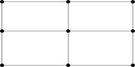
Figure 1: Graph $J_{2,4}$

We have to determine $\sigma(J_{2,4})_{k}$, for $k=1,2,3,4$.
Let $k=1$.
By the cutting-down method, it easily results:  $4\,(2\cdot 4)=32$ .
Let $k=2$.
Let $B$ be the $4\choose 2$ $\!\!\times 2$ matrix  $\left(\begin{array}[]{cc}1&2\\ 1&3\\ 1&4\\ 2&3\\ 2&4\\ 3&4\end{array}\right)$; the matrix $C$ will be  $\left(\begin{array}[]{cc}0&2\\ 1&1\\ 0&2\\ 0&2\\ 1&1\\ 0&2\end{array}\right)$ .
The number of equivalence classes of the spanning trees with two common edges in $J_{2,4}$ is 2, that is the number of distinct rows of $C$. In particular, the row $C[1]=(0\;\;2)$ repeats itself $4$ times, the row $C[2]=(1\;\;1)$ repeats itself $2$ times.
The contribution of the spanning trees related to $C[1]$ is   $s_{1}=2^{2}\cdot 1\cdot 3=12$ ;   that one related to $C[2]$ is   $s_{2}=2^{2}\cdot 2\cdot 2=16$ . Therefore the number of the spanning trees of $J_{2,4}$ with two common edges is  $\sigma(J_{2,4})_{2}=4\cdot 12+2\cdot 16=80$.
Let $k=3$.
Let $B$ be the $4\choose 3$ $\!\!\times 2$ matrix $\left(\begin{array}[]{ccc}1&2&3\\ 1&2&4\\ 1&3&4\\ 2&3&4\end{array}\right)$; the matrix $C$ will be $\left(\begin{array}[]{ccc}0&0&1\\ 0&0&1\\ 0&0&1\\ 0&0&1\end{array}\right)$ .
The 4 rows of $C$ are the same, so the contribution of the spanning trees is  $2^{3}\cdot 1\cdot 1\cdot 2=16$  and $\sigma(J_{2,4})_{3}=4\cdot 16=64$.
Let $k=4$.
This case is trivial; in fact, $B$ is the row matrix  $(1\;\;2\;\;3\;\;4)$  and $C$ the row matrix $(0\;\;0\;\;0\;\;0)$. Consequently  $\sigma(J_{2,4})_{4}=2^{4}=16$.
In conclusion, $\sigma(J_{2,4})=32+80+64+16=192$ .

The strength of the algorithmic description introduced for the calculation of spanning trees of any Jahangir graph lies in the fact that with simple operations between integers we can model the totality of dispositions which assume the common edges of the inner cycles $C_{n+2}$ of the graph.
Thus we have examined an alternative method which, in the case of this type of graphs, qualitatively and quantitatively solves the problem of determining the spanning trees. It is significant to observe that, by applying the Matrix Tree Theorem, only the total number of such trees is determined, indeed through this algorithm are also found all the possible graphs which originate from the given graph after applying the cutting-down method.

The source code of the algorithm
Following the Example 2.1, we execute the algorithm for the computation of $\sigma(J_{n,m})_{k}$ in PHP programming language.
$<$?php
$n$=$2;
$m$=$4;
$k$=$3;
class Combinations implements Iterator
{
  protected $c$=$null;
  protected $s$=$null;
  protected $n$=$0;
  protected $k$=$0;
  protected $pos$=$0;
  function $\_\!\_\,\_\!\_$construct($s, $k) {
    if(is$\_\!\_$array($s)) {
    $this$-\!\!>$s$=$array$\_\!\_$values($s);
    $this$-\!\!>$n$=$count($this$-\!\!>$s);
    } else {
    $this$-\!\!>$s$=$(string) $s;
    $this$-\!\!>$n$=$strlen($this$-\!\!>$s);
   }
   $this$-\!\!>$k$=$$k;
   $this$-\!\!>$rewind();
   }
  function key() {
    return $this$-\!\!>$pos;
  }
  function current() {
   $r$=$array();
    for($i$=$0; $i$<$$this$-\!\!>$k; $i++)
    $r[ ]$=$$this$-\!\!>$s[$this$-\!\!>$c[$i]];
    return is$\_\!\_$array($this$-\!\!>$s) ? $r : implode(",$r);
   }
  function next() {
    if($this$-\!\!>$$\_\!\_$next())
    $this$-\!\!>$pos++;
    else
    $this$-\!\!>$pos$=-$1;
  }
  function rewind() {
    $this$-\!\!>$c$=$range(0, $this$-\!\!>$k);
    $this$-\!\!>$pos$=$0;
  }
  function valid() {
    return $this$-\!\!>$pos$>=$0;
  }
   protected function $\_\!\_$next() {
    $i$=$$this$-\!\!>$k$-$1;
    while ($i$>=$0 && $this$-\!\!>$c[$i] $==$ $this$-\!\!>$n$-$$this$-\!\!>$k+$i)$i$--$;
    if($i$<$0)
    return false;
   $this$-\!\!>$c[$i]++;
    while($i$++<$$this$-\!\!>$k$-$1)
    $this$-\!\!>$c[$i]$=$$this$-\!\!>$c[$i$-$1]+1;
   return true;
  }
}
$s $=$ "";
for($c$=$1; $c$<=$ $m; $c++) {
   $s .$=$ $c."$-$";
}
$s$=$substr($s, 0, strlen($s)$-$1);
$b$=$array();
$combs$=$new Combinations(explode("$-$",$s), $k);
echo "$\backslash$n----------------------------------------------------------$\backslash$n";
echo "BINOMIAL ($m $k):".iterator$\_\!\_$count($combs)."$\backslash$n$\backslash$n";
foreach($combs as $substring) {
  $b[ ]$=$$substring;
  //echo implode("",$substring)."$\backslash$n";
}
  /$\ast\ast$
$g$=$array();
foreach($b as $row) {
}$\ast$/
$g$=$array();
$countB$=$count($b);
for($j$=$0; $j$<$$countB; $j++) {
   for($i$=$0; $i$<$($k$-$1); $i++) {
     $g[$j][$i]$=$$b[$j][$i+1]$-$$b[$j][$i]$-$1;
   }
   $g[$j][$k$-$1]$=$$b[$j][0]+$m$-$$b[$j][$k$-$1]$-$1;
   sort($g[$j]);
}
unset($b);
for($i$=$0; $i$<$$countB; $i++) {
   $g[$i]$=$implode("$-$",$g[$i]);
}
echo "$\backslash$n----------------------------------------------------------";
echo "$\backslash$nCOUNTING OCCURRENCES OF IDENTICAL STRUCTURES (GAMMA): $\backslash$n$\backslash$n";
$final$=$array$\_\!\_$count$\_\!\_$values($g);
unset($g);
//return keys as values, these are the counters
print$\_\!\_$r($final);
$occurrences$=$array$\_\!\_$keys($final);
$constants$=$array();
for($j$=$0; $j$<$count($occurrences); $j++) {
   $ris$=$1;
   $chars$=$explode("$-$", $occurrences[$j]);
   for($i$=$0; $i$<$$k; $i++) {
     $ris$=$$ris $\ast$ ($chars[$i]+1);
   }
   //echo "$\backslash$n-------".($ris)."-------$\backslash$n";
   $ris$=$$ris$\ast$pow($n,$k);
   $constants[ ]$=$array($occurrences[$j], $ris);
}
echo "$\backslash$n----------------------------------------------------------";
echo "$\backslash$nCONSTANTS (c):$\backslash$n$\backslash$n";
print$\_\!\_$r($constants);
$total$=$0;
$counts$=$array$\_\!\_$values($final);
for($a$=$0; $a$<$count($occurrences); $a++) {
   $total$=$$total+($counts[$a]$\ast$$constants[$a][1]);
}
echo "SPANNING TREES of J($n, $m), with $k common edges:".$total."$\backslash$n";

An application on secure data transmission
Graphs are geometric models for several problems in which there are sets with links among the elements. For this reason a graph can be employed to analyze connection problems in different fields.
Here we explain how the algebraic and geometric models built through graph theory in the paper and the procedures to determine the spanning trees of Jahangir graphs are good instruments for transmitting confidential information. More precisely we describe an application of data transmission arising from real security problems. It is necessary to communicate the type of arming situated inside on some nuclear sites in a country.

The nuclear sites are located and we can represent them through the vertex set of the above considered simple connected graph $\mathcal{G}$:

We may build all subtrees $\mathcal{G}_{i}$ of $\mathcal{G}$ that contain each vertex of $\mathcal{G}$ .
The role of the supporting graphs $\mathcal{G}_{i}$ is of fundamental importance in transmitting protected data.

The nuclear sites are known and represented by the finite vertex set of $\mathcal{G}$. The arming is classified through the vertex set of unknown graphs $\mathcal{G}_{i}$. The message to be sent is the graph $\mathcal{G}$ and each $\mathcal{G}_{i}$ contains the real meaning of the message because its edges give the connection between the nuclear sites and their arming. The receiver will get acquainted with the type of arming placed in every site applying the algebraic procedure to build $\mathcal{G}_{i}$ .
In our case $\mathcal{G}$ is the Jahangir graph $J_{n,m}$. We associate to $\mathcal{G}$ the subgraphs $\mathcal{G}_{i}$, that are its spanning trees computed through the described procedure. Hence we can represent the nuclear sites through the vertex set of the connected graph $J_{n,m}$. The transmitter sends in his message the drawing of the graph $J_{n,m}$. The receiver will elaborate the potential information contained in it computing the spanning trees $\mathcal{G}_{i}$ .

3 On some relationships between the $\sigma(J_{n,m})$

Let’s study another aspect of the class of Jahangir graphs $J_{n,m}$ in relation to the calculation of the spanning trees of them.
We will want to locate the general structure of the class of Jahangir graphs. Recall that for any Jahangir graph $J_{n,m}$ the index $n$ is the number of edges that each inner cycle of it does not share with other inner cycles, while the index $m$ is the number of inner cycles interiors that make up the graph.
Considering the totality of Jahangir graphs, it is interesting to study those who have the same first or second index.
Taken for example the Jahangir graphs for which $m=3$ and calculating the spanning trees on the ground of the number of common edges which they present, we can write:

$\sigma(J_{n,3})=\sigma(J_{n,3})_{3}+\sigma(J_{n,3})_{2}+\sigma(J_{n,3})_{1}=n^{3}+3(2n)n^{3-2}+3(3n)$ .
Now introduce a statement that shows the relationship between the spanning trees related to two Jahangir graphs whose first indices are consecutive numbers.

Theorem 3.1.

Let $m\in{\mathbb{N}}$ and $m>2$. Then  $\displaystyle{\lim_{n\to\infty}\frac{\sigma(J_{n,m})}{\sigma(J_{n-1,m})}=1}$.

Proof.

For a fixed positive integer $m>2$ it results that:

$$\sigma(J_{n,m})=\sum_{k=1}^{m}\sigma(J_{n,m})_{k}=n^{m}+\sum_{i=1}^{m-1}c_{i}n^{i},\,\mathrm{for\,\,}c_{i}\in{\mathbb{R}}\,.$$

Consequently  $\displaystyle{\lim_{n\to\infty}\frac{\sigma(J_{n,m})}{\sigma(J_{n-1,m})}=\lim_{n\to\infty}\frac{n^{m}+\sum_{i=1}^{m-1}c_{i}n^{i}}{(n-1)^{m}+\sum_{i=1}^{m-1}c_{i}(n-1)^{i}}=1.}$ ∎

Observe that the theorem holds even for two non-consecutive values of the first indices.
The previous result emphasizes the geometric and analytical aspect of the problem: in fact, it appears that the number of spanning trees of Jahangir graphs having the same second index and the first one tending to infinity, tends to be a constant.
It may be noted, explaining the calculation, that the limit function is decreasing: geometrically this means that spanning trees of Jahangir graphs $J_{n,m}$ , with $m$ constant and $n$ large enough, turn out to be almost in equal number; in other words, fixing the number of edges connected to the central vertex, it is as if we were tending a polygonal to an arc of circumference increasing its edges.
This leads to the conclusion that, after a certain index $n\!\gg\!0,\,\sigma(J_{n,m})$ and $\sigma(J_{n-1,m})$ tend to assume values very close to each other.
Experimentally, instead, doing a similar study on the increase in value of the second index of a Jahangir graph $J_{n,m}$ fixed the first one, it results that the fraction between the number of spanning trees related to two Jahangir graphs whose second indices are consecutive numbers, for $m$ tending to infinity, seems to approximate to a constant, different for each choice of $n$.
First, let’s analyze the behaviour of the spanning trees of the Jahangir graphs $J_{2,m}$ and $J_{3,m}$, for $m\geq 3$.

$m$	$\sigma(J_{2,m})$	$\sigma(J_{3,m})$
3	50	108
4	192	525
5	722	2523
6	2700	12096
7	10082	57963
8	37632	277725
9	140450	1330668
10	524172	6375621
11	1956242	30547443
12	7300800	146361600
13	27246962	701260563
14	101687052	3359941221
15	379501250	16098445548
16	1416317952	77132286525
…	………	………

Known such information, now we wonder if it is possible to compute $\sigma(J_{2,m})$ or $\sigma(J_{3,m})$, for any $m$, namely in general if it is possible to identify a relationship among the number of spanning trees of $\sigma(J_{n,m})$, when $n\geq 2$ is assigned. To this end we introduce the sequences:

$\displaystyle{a_{2,m}=\frac{\sigma(J_{2,m+1})}{\sigma(J_{2,m})}},$  con $m\in{\mathbb{N}},\,m\geq 3\,,$

$\displaystyle{a_{3,m}=\frac{\sigma(J_{3,m+1})}{\sigma(J_{3,m})}},$  con $m\in{\mathbb{N}},\,m\geq 3\,.$

Building sequences of the mentioned type, for any fixed integer $n\geq 2$, that is, considering a countable infinity of sequences, it does highlight a symmetry that can already be grasped visually. Formalizing a relation between these numbers, the way in which the problem numerically evolves can be analyzed.
The values of the first terms of the two sequences introduced above, for all $m$, are the following:

$m$	$a_{2,m}$	$a_{3,m}$
3	3,84	4,86
4	3,7604	4,8057
5	3,7396	4,7943
6	3,7340	4,7919
7	3,732593	4,791418
8	3,732196	4,791315
9	3,7320897	4,7912935
10	3,7320612	4,7912890
11	3,732053600	4,7912880
12	3,732051556	4,791287899
13	3,732051008	4,791287858
14	3,732050861	4,7912878497
15	3,732050822	4,7912878479
…	………	………

It is evident that, for any fixed $n\geq 2$ and for any variation of the second index $m$, the number of spanning trees tend to have a linear increase.
In particular, for $n=2$ we can introduce a constant $\delta_{2}$ and conjecture the existence of the following:

$\displaystyle{\lim_{m\to+\infty}a_{2,m}}=\delta_{2}\sim 3,732050...$
For $n=3$, analogously, we can introduce a constant $\delta_{2}$ and conjecture the existence of the following:

$\displaystyle{\lim_{m\to+\infty}a_{3,m}}=\delta_{3}\sim 4,791287...$
And so on, for any increase of $n$. Then we can formulate the following

Conjecture 3.1.

Let $n,m\in{\mathbb{N}}$ and $n\geq 2$ fixed. Let $a_{n,m}=\displaystyle{\frac{\sigma(J_{n,m+1})}{\sigma(J_{n,m})}}\,.$ Then it is,

$\displaystyle{\lim_{m\to+\infty}a_{n,m}}=\delta_{n}$,   where  $\delta_{n}\in{\mathbb{R}}$ .
Moreover,

$\sigma(J_{n,m})=(\delta_{n})^{m-3}\,\sigma(J_{n,3})\,.$

It follows that, for each $\delta_{n}$, to know the number of spanning trees of the Jahangir graphs $J_{n,m}$ it is enough to know exactly $\sigma(J_{n,3})$ .

Acknowledgements
We thank engineer Alberto Ruffo for the fruitful job in implementing the PHP code.
The research that led to the present paper was partially supported by a grant of the group GNSAGA of INdAM, Italy.

References

- [1] Anwar, I., Raza, Z., Kashif, A. - Spanning simplicial complexes of uni-cyclic graphs. Alg. Colloq., 22, 4 (2015), 707–710.
- [2] Anwar, I., Raza, Z., Kashif, A. - On the algebraic study of spanning simplicial complex of -cyclic graphs . Ars Comb., 115 (2014), 89–99.
- [3] Boomen, J. - The matrix tree theorem. Master Thesis, 2007.
- [4] Harary, F. - Graph Theory. Addison-Wesley, Reading, MA, 1994.
- [5] Imbesi, M. - Integrality of the symmetric algebra of graphs ideals. Math. Notes, 94, 2 (2013), 191–204.
- [6] Imbesi, M., La Barbiera, M. - Algebraic properties of non-squarefree graph ideals. Math. Rep., 15(65), 2 (2013), 107–113.
- [7] Imbesi, M., La Barbiera, M. - Invariants of symmetric algebras associated to graphs. Turk. J. Math., 36, 3 (2012), 345–358.
- [8] Imbesi, M., La Barbiera, M. - Theoretic properties of the symmetric algebra of edge ideals. Bull. Belg. Math. Soc. Sim., 22, 2 (2015), 331–342.
- [9] Imbesi, M., La Barbiera, M., Tang, Z. - On the graphic realization of certain monomial sequences. J. Alg. Appl., 14, 5 (2015) 1550073, 9 pages.
- [10] Kashif, A., Raza, Z., Anwar, I. - Algebraic characterization of the SSC . ArXiv: 1509.04307v2 (2016).
- [11] Kirchhoff, G. - Über die Auflösung der Gleichungen, auf welche man bei der untersuchung der linearen verteilung galvanischer Ströme geführt wird. Ann. Phys. Chem., 72 (1847), 497- 508.
- [12] Lourdusamy, A., Jeyaseelan, S.S., Mathivanan, T. - On pebbling Jahangir graph. Gen. Math. Notes, 5, 2 (2011), 42–49.
- [13] Saraceno, S. - Un approccio algebrico combinatorico per la determinazione degli alberi ricoprenti di grafi di Jahangir. Degree Thesis, 2015.
- [14] Villarreal, R.H. - Monomial Algebras. M. Dekker Inc., New York, Pure and Appl. Math. 238, 2001.