One-loop perturbative coupling of $A$ and $A_{\star}$ through the chiral overlap operator

Abstract

We study the one-loop effective action defined by the chiral overlap operator in the four-dimensional lattice formulation of chiral gauge theories by Grabowska and Kaplan. In the tree-level continuum limit, the left-handed component of the fermion is coupled only to the original gauge field $A$, while the right-handed one is coupled only to $A_{\star}$, which is given by the gradient flow of $A$ with infinite flow time. In this paper, we show that the continuum limit of the one-loop effective action contains local interaction terms between $A$ and $A_{\star}$, which do not generally vanish even if the gauge representation of the fermion is anomaly free. We argue that the presence of such interaction terms can be regarded as undesired gauge symmetry-breaking effects in the formulation.

B01, B05, B31, B57

1 Introduction and discussion

Recently, Grabowska and Kaplan constructed a four-dimensional lattice formulation of chiral gauge theories Grabowska:2016bis , starting from their five-dimensional domain-wall formulation in Ref. Grabowska:2015qpk . A salient feature of this formulation is that the lattice Dirac operator depends on two gauge fields: one is the original gauge field $A$, and the other is $A_{\star}$, which is given by the gradient flow Narayanan:2006rf ; Luscher:2009eq ; Luscher:2010iy ; Luscher:2011bx of $A$ with infinite flow time. In the tree-level continuum limit of the formulation, the left-handed component of the fermion is coupled only to $A$, while the right-handed one (called the fluffy mirror fermion or “fluff”) is coupled only to $A_{\star}$. Up to a subtlety associated with the topological charge Grabowska:2015qpk ; Grabowska:2016bis ; Okumura:2016dsr ; Makino:2016auf , $A_{\star}$ basically becomes pure gauge after the infinite-time flow. Then this setup would be regarded as the system of the left-handed Weyl fermion coupled to the gauge field $A$ (in the spirit of Ref. AlvarezGaume:1983cs ). Since the flow equation preserves the gauge covariance Narayanan:2006rf ; Luscher:2009eq ; Luscher:2010iy ; Luscher:2011bx , $A_{\star}$ transforms gauge covariantly under the gauge transformation. Then the fermion determinant is manifestly gauge invariant in this formulation, even if the gauge representation is anomalous. It is crucial to understand, therefore, how this formulation fails when the gauge representation is anomalous. It is conceivable that the locality plays a key role for this but no definite argument has been given yet.

So far, the explicit form of the four-dimensional lattice Dirac operator in the above formulation has been obtained only when the transition from $A$ to $A_{\star}$ along the flow is “abrupt” or “sudden”; the resulting Dirac operator is referred to as the chiral overlap operator in the present paper and is denoted by $\hat{\mathcal{D}}_{\chi}$. As noted above, in the tree-level continuum limit Grabowska:2016bis ,

$$am\hat{\mathcal{D}}_{\chi}\stackrel{{\scriptstyle a\to 0}}{{\to}}\gamma_{\mu}D_{\mu}(A)P_{-}+\gamma_{\mu}D_{\mu}(A_{\star})P_{+},$$ (1.1)

where $a$ is the lattice spacing, $m$ is a parameter of mass dimension one, $D_{\mu}(A)$ ($D_{\mu}(A_{\star})$) is the covariant derivative defined with $A$ ($A_{\star}$), $\gamma_{\mu}$ is the Dirac matrix, and $P_{\pm}=(1\pm\gamma_{5})/2$ are the chirality projection operators. Thus, the lattice Dirac operator does not produce any coupling between two gauge fields, $A$ and $A_{\star}$, in the tree-level approximation.

In this paper, we investigate how the above situation is modified under radiative corrections. We thus study the fermion one-loop effective action defined by

$$\ln\mathcal{Z}[A,A_{\star}]\equiv\ln\int\prod_{x}\left[d\psi(x)d\bar{\psi}(x)\right]\exp\left[-a^{4}\sum_{x}\bar{\psi}(x)\hat{\mathcal{D}}_{\chi}\psi(x)\right],$$ (1.2)

where the two gauge fields $A$ and $A_{\star}$ are regarded as independent non-dynamical variables. In the present paper, we assume that the gauge field is perturbative and the Dirac operator has no normalizable zero modes. What we will show in this paper is

$$\delta\delta_{\star}\ln\mathcal{Z}[A,A_{\star}]=-\int d^{4}x\,\mathcal{L}(A,A_{\star};\delta A,\delta_{\star}A_{\star})$$ (1.3)

in the continuum limit, where $\mathcal{L}(A,A_{\star};\delta A,\delta_{\star}A_{\star})$ is a local polynomial of its arguments and their spacetime derivatives. In this expression and in what follows, the infinitesimal variation $\delta$ acts only on $A$ but not on $A_{\star}$,

$$\delta A\neq 0,\qquad\delta A_{\star}\equiv 0,$$ (1.4)

while $\delta_{\star}$ acts in an opposite way,

$$\delta_{\star}A\equiv 0,\qquad\delta_{\star}A_{\star}\neq 0.$$ (1.5)

Equation (1.3) tells us that through fermion one-loop diagrams, two gauge fields $A$ and $A_{\star}$ acquire local couplings. The locality of $\mathcal{L}(A,A_{\star};\delta A,\delta_{\star}A_{\star})$ is expected because in the lattice Dirac operator $\hat{\mathcal{D}}_{\chi}$ the coupling between $A$ and $A_{\star}$ is $O(a)$ and thus the coupling emerges only through ultraviolet divergences. We will further find that $\mathcal{L}(A,A_{\star};\delta A,\delta_{\star}A_{\star})$ does not vanish even if the gauge representation of the fermion is anomaly free.

What is a possible implication of our observation (1.3)? To find this, let us classify the terms in $\ln\mathcal{Z}[A,A_{\star}]$ according to their dependences as,

$$\ln\mathcal{Z}[A,A_{\star}]={\mit\Gamma}_{0}[A]+{\mit\Gamma}_{1}[A,A_{\star}]+{\mit\Gamma}_{2}[A_{\star}],$$ (1.6)

where ${\mit\Gamma}_{1}[A,A_{\star}]$ consists of cross terms between $A$ and $A_{\star}$. Equation (1.3) thus shows that

$$\delta\delta_{\star}{\mit\Gamma}_{1}[A,A_{\star}]=-\int d^{4}x\,\mathcal{L}(A,A_{\star};\delta A,\delta_{\star}A_{\star})$$ (1.7)

in the continuum limit. On the other hand, by construction (1.2), the effective action is invariant under the gauge transformation, if we gauge-transform both $A$ and $A_{\star}$ Grabowska:2016bis . Expressing the gauge variations by a superscript as

$$\delta^{\omega}A_{\mu}(x) \equiv\partial_{\mu}\omega(x)+[A_{\mu}(x),\omega(x)], \delta^{\omega}A_{\star\mu}(x) =0,$$ (1.8)

$$\delta_{\star}^{\omega}A_{\star\mu}(x) \equiv\partial_{\mu}\omega(x)+[A_{\star\mu}(x),\omega(x)], \delta_{\star}^{\omega}A_{\mu}(x) =0,$$ (1.9)

the gauge invariance implies

$$(\delta^{\omega}+\delta_{\star}^{\omega})\ln\mathcal{Z}[A,A_{\star}]=0\Rightarrow\delta(\delta^{\omega}+\delta_{\star}^{\omega})\ln\mathcal{Z}[A,A_{\star}]=0.$$ (1.10)

Then, using Eqs. (1.6) and (1.7) in this relation, we have

$$\delta\delta^{\omega}{\mit\Gamma}_{0}[A]+\delta\delta^{\omega}{\mit\Gamma}_{1}[A,A_{\star}]=-\delta\delta_{\star}^{\omega}{\mit\Gamma}_{1}[A,A_{\star}]=\int d^{4}x\,\mathcal{L}(A,A_{\star};\delta A,\delta_{\star}^{\omega}A_{\star}).$$ (1.11)

Now, the gauge field $A_{\star}$ is given by the gradient flow of $A$ for infinite flow time. Thus, let us assume that $A_{\star}$ is pure gauge. Although there exists a subtlety as to whether this is actually the case or not for topologically non-trivial gauge field configurations Grabowska:2016bis ; Okumura:2016dsr , this will certainly be the case for topologically trivial configurations. Under this assumption, since the lattice gauge action $S_{G}[A]$ (such as the plaquette action) with which the gauge field $A$ is integrated over will be gauge invariant, we may take a particular gauge in which $A_{\star}\equiv 0$. In this $A_{\star}=0$ gauge, since ${\mit\Gamma}_{1}[A,A_{\star}]$ and ${\mit\Gamma}_{2}[A_{\star}]$ in Eq. (1.6) are constants, from Eqs. (1.6) and (1.11), we have

$$\delta\delta^{\omega}\ln\mathcal{Z}[A,0]=\int d^{4}x\,\mathcal{L}(A,A_{\star}=0;\delta A,\delta_{\star}^{\omega}A_{\star}|_{A_{\star}=0}).$$ (1.12)

We will see that the right-hand side does not vanish even if the gauge representation is anomaly free. Thus, generally, configurations of the gauge field $A$ (in a topologically trivial sector) are integrated with the sum of the gauge-invariant action $S_{G}[A]$ and gauge non-invariant effective action $\ln\mathcal{Z}[A,0]$. For example, we will see that $\mathcal{L}(A,A_{\star}=0;\delta A,\delta_{\star}^{\omega}A_{\star}|_{A_{\star}=0})$ contains a term corresponding to the mass term of the gauge field. Such gauge-breaking effects which are not related to the gauge anomaly should be able to be removed by local counterterms. This expectation is explicitly confirmed in Appendix A. Nevertheless, such a necessity for counterterms to restore the gauge symmetry will be undesirable for a possible non-perturbative formulation of chiral gauge theories. This is the implication of our observation (1.3). It appears that the formulation of Ref. Grabowska:2016bis with the chiral overlap operator $\hat{\mathcal{D}}_{\chi}$ (i.e., the sudden flow case) should be improved in some possible way. In the rest of this paper, we will explain how Eq. (1.7) is obtained.

2 Computation of Eq. (1.7)

2.1 Basic formulation

The explicit form of the chiral overlap operator $\hat{\mathcal{D}}_{\chi}$ is given by Grabowska:2016bis ,

$$a\hat{\mathcal{D}}_{\chi}=1+\gamma_{5}\left[1-(1-\epsilon_{\star})\frac{1}{\epsilon\epsilon_{\star}+1}(1-\epsilon)\right],$$ (2.1)

where $\epsilon$ and $\epsilon_{\star}$ are the sign functions Neuberger:1997fp ; Neuberger:1998wv

$$\epsilon\equiv\frac{H_{w}(A)}{\sqrt{H_{w}(A)^{2}}},\qquad\epsilon_{\star}\equiv\frac{H_{w}(A_{\star})}{\sqrt{H_{w}(A_{\star})^{2}}}$$ (2.2)

of the Hermitian Wilson–Dirac operator

$$H_{w}=\gamma_{5}\left[\frac{1}{2}\gamma_{\mu}(\nabla_{\mu}+\nabla_{\mu}^{*})-\frac{1}{2}a\nabla_{\mu}\nabla_{\mu}^{*}-m\right],$$ (2.3)

where $\nabla_{\mu}$ and $\nabla_{\mu}^{*}$ are forward and backward gauge covariant lattice derivatives, respectively. The parameter $m$ is taken as $0<am<2$. From Eq. (2.2), $\epsilon$ depends only on the gauge field $A$ and $\epsilon_{\star}$ only on $A_{\star}$. By construction,

$$\epsilon^{2}=\epsilon_{\star}^{2}=1.$$ (2.4)

Using these, one can confirm that

$$\left[1-(1-\epsilon_{\star})\frac{1}{\epsilon\epsilon_{\star}+1}(1-\epsilon)\right]^{2}=1$$ (2.5)

and, consequently, $\hat{\mathcal{D}}_{\chi}$ in Eq. (2.1) satisfies the Ginsparg–Wilson relation Ginsparg:1981bj

$$\gamma_{5}\hat{\mathcal{D}}_{\chi}+\hat{\mathcal{D}}_{\chi}\gamma_{5}=a\hat{\mathcal{D}}_{\chi}\gamma_{5}\hat{\mathcal{D}}_{\chi}.$$ (2.6)

It is then natural to introduce a modified $\gamma_{5}$ Luscher:1998pqa ; Niedermayer:1998bi ,

$$\hat{\gamma}_{5}\equiv\gamma_{5}(1-a\hat{\mathcal{D}}_{\chi}),$$ (2.7)

which satisfies

$$(\hat{\gamma}_{5})^{2}=1,\qquad\hat{\mathcal{D}}_{\chi}\hat{\gamma}_{5}=-\gamma_{5}\hat{\mathcal{D}}_{\chi}.$$ (2.8)

Note, however, that $\hat{\gamma}_{5}$ is not Hermitian in the present formulation, $\hat{\gamma}_{5}^{\dagger}\neq\hat{\gamma}_{5}$. From the first relation of Eq. (2.8), one can define modified chiral projection operators by

$$\hat{P}_{\pm}\equiv\frac{1}{2}(1\pm\hat{\gamma}_{5}).$$ (2.9)

The chiral components of the fermion can then be defined as

$$\hat{P}_{-}\psi_{L}(x) =\psi_{L}(x), \bar{\psi}_{L}(x)P_{+}=\bar{\psi}_{L}(x),$$ (2.10)

$$\hat{P}_{+}\psi_{R}(x) =\psi_{R}(x), \bar{\psi}_{R}(x)P_{-}=\bar{\psi}_{R}(x).$$ (2.11)

Thanks to the second relation of Eq. (2.8), the action is completely decomposed into the left-handed and right-handed components as

$$a^{4}\sum_{x}\bar{\psi}(x)\hat{\mathcal{D}}_{\chi}\psi(x)=a^{4}\sum_{x}\left[\bar{\psi}_{L}(x)\hat{\mathcal{D}}_{\chi}\psi_{L}(x)+\bar{\psi}_{R}(x)\hat{\mathcal{D}}_{\chi}\psi_{R}(x)\right].$$ (2.12)

2.2 Gauge currents and partial decoupling of the right-handed fluff fermion

In the present paper, we assume that the gauge field is perturbative and the Dirac operator has no normalizable zero modes in infinite volume. Then the change of the effective action (1.2) under the variation of the gauge field $\delta$ (1.4), for example, is given by

$$\delta\ln\mathcal{Z}[A,A_{\star}] =-a^{4}\sum_{x}\left\langle\bar{\psi}(x)\delta\hat{\mathcal{D}}_{\chi}\psi(x)\right\rangle$$

$$=\operatorname{Tr}\delta\hat{\mathcal{D}}_{\chi}\frac{1}{\hat{\mathcal{D}}_{\chi}},$$ (2.13)

where $\operatorname{Tr}\equiv\sum_{x}\operatorname{tr}$ and $\operatorname{tr}$ stands for the trace over the spinor and gauge indices. In deriving this, we have used the fermion propagator,

$$\left\langle\psi(x)\bar{\psi}(y)\right\rangle=\frac{1}{\hat{\mathcal{D}}_{\chi}}\frac{1}{a^{4}}\delta_{x,y}.$$ (2.14)

We will refer to Eq. (2.13) (and a similar expression for the variation $\delta_{\star}$ (1.5)) as the “gauge current.” Because of Eq. (2.8), we may decompose the gauge current (2.13) into two parts by inserting chiral projectors:

$$\operatorname{Tr}\delta\hat{\mathcal{D}}_{\chi}\frac{1}{\hat{\mathcal{D}}_{\chi}}=\operatorname{Tr}\delta\hat{\mathcal{D}}_{\chi}\hat{P}_{-}\frac{1}{\hat{\mathcal{D}}_{\chi}}P_{+}+\operatorname{Tr}\delta\hat{\mathcal{D}}_{\chi}\hat{P}_{+}\frac{1}{\hat{\mathcal{D}}_{\chi}}P_{-}.$$ (2.15)

In the right-hand side of this expression, the first term can be regarded as a collection of one-loop diagrams of the physical left-handed fermion containing at least one interaction vertex with $A$. Similarly, the second term can be regarded as a collection of similar one-loop diagrams but of the right-handed fluff fermion.

Interestingly, the last term of Eq. (2.15) identically vanishes even with finite lattice spacings. This might be regarded as a (partial) decoupling of the fluff fermions from the physical gauge field $A$ in the one-loop level; this is certainly a desired property. To see this, we first note that because of $\epsilon^{2}=\epsilon_{\star}^{2}=1$ the chiral overlap operator (2.1) can be written as

$$a\hat{\mathcal{D}}_{\chi}=1+\gamma_{5}\left[1-2(1-\epsilon_{\star})\frac{1}{\epsilon\epsilon_{\star}+1}\right].$$ (2.16)

Then since $\delta$ (1.4) does not change $\epsilon_{\star}$, noting again that $\epsilon^{2}=\epsilon_{\star}^{2}=1$ (and thus $\delta\epsilon\epsilon=-\epsilon\delta\epsilon$), we have the following sequence of equalities:

$$\delta a\hat{\mathcal{D}}_{\chi} =2\gamma_{5}(1-\epsilon_{\star})\frac{1}{\epsilon\epsilon_{\star}+1}\delta\epsilon\epsilon_{\star}\frac{1}{\epsilon\epsilon_{\star}+1}$$

$$=\gamma_{5}(1-\epsilon_{\star})(1-\epsilon_{\star})\frac{1}{\epsilon\epsilon_{\star}+1}\delta\epsilon\epsilon_{\star}\frac{1}{\epsilon\epsilon_{\star}+1}$$

$$=\gamma_{5}(1-\epsilon_{\star})\frac{1}{\epsilon\epsilon_{\star}+1}(1-\epsilon)\delta\epsilon\epsilon_{\star}\frac{1}{\epsilon\epsilon_{\star}+1}$$

$$=\gamma_{5}(1-\epsilon_{\star})\frac{1}{\epsilon\epsilon_{\star}+1}\delta\epsilon(1+\epsilon)\epsilon_{\star}\frac{1}{\epsilon\epsilon_{\star}+1}$$

$$=\gamma_{5}(1-\epsilon_{\star})\frac{1}{\epsilon\epsilon_{\star}+1}\delta\epsilon\epsilon_{\star}\frac{1}{\epsilon\epsilon_{\star}+1}(1+\epsilon_{\star}).$$ (2.17)

On the other hand, from Eqs. (2.9), (2.7), and (2.1), we have

$$\hat{P}_{+}=\frac{1+\hat{\gamma}_{5}}{2}=\frac{1}{2}(1-\epsilon_{\star})\frac{1}{\epsilon\epsilon_{\star}+1}(1-\epsilon).$$ (2.18)

These show that

$$\delta a\hat{\mathcal{D}}_{\chi}\hat{P}_{+}=0$$ (2.19)

and thus the last term of Eq. (2.15) identically vanishes. That is,

$$\operatorname{Tr}\delta\hat{\mathcal{D}}_{\chi}\frac{1}{\hat{\mathcal{D}}_{\chi}}=\operatorname{Tr}\delta\hat{\mathcal{D}}_{\chi}\hat{P}_{-}\frac{1}{\hat{\mathcal{D}}_{\chi}}P_{+},\qquad\operatorname{Tr}\delta\hat{\mathcal{D}}_{\chi}\hat{P}_{+}\frac{1}{\hat{\mathcal{D}}_{\chi}}P_{-}=0.$$ (2.20)

As relations being dual to these, we also have

$$\operatorname{Tr}\delta_{\star}\hat{\mathcal{D}}_{\chi}\frac{1}{\hat{\mathcal{D}}_{\chi}}=\operatorname{Tr}\delta_{\star}\hat{\mathcal{D}}_{\chi}\hat{P}_{+}\frac{1}{\hat{\mathcal{D}}_{\chi}}P_{-},\qquad\operatorname{Tr}\delta_{\star}\hat{\mathcal{D}}_{\chi}\hat{P}_{-}\frac{1}{\hat{\mathcal{D}}_{\chi}}P_{+}=0.$$ (2.21)

2.3 Functional curl

The structure of the “gauge current” (2.20) is quite analogous to the covariantly regularized gauge current of the left-handed Weyl fermion Fujikawa:1983bg , which leads to the covariant gauge anomaly Bardeen:1984pm . This definition of the gauge current preserves the gauge covariance even for anomalous cases at the expense of the Bose symmetry in fermion one-loop diagrams. The Bose symmetry is restored (in the continuum theory) if the gauge representation of the Weyl fermion is anomaly free. The breaking of the Bose symmetry can be characterized by the “functional curl”; this notion appears in various places in consideration of the anomaly—see for example, Ref. Banerjee:1986bu and Sect. 6.6 of Ref. Fujikawa:2004cx . In our present problem, the analogue of the functional curl (associated with the right-handed fluff fermion) would be

$$\delta_{\star}\operatorname{Tr}\delta\hat{\mathcal{D}}_{\chi}\hat{P}_{+}\frac{1}{\hat{\mathcal{D}}_{\chi}}P_{-}-\delta\operatorname{Tr}\delta_{\star}\hat{\mathcal{D}}_{\chi}\hat{P}_{+}\frac{1}{\hat{\mathcal{D}}_{\chi}}P_{-}.$$ (2.22)

We expect that in the continuum limit this combination becomes local because if we neglect the subtlety associated with the definition of the gauge current in quantum theory (such as the covariant versus consistent), then the gauge current would always be given by the derivative of the effective action and then the combination such as Eq. (2.22) would vanish. We will shortly see that this expectation is correct. Note that Eqs. (2.20), (2.21) and (2.13) with $\delta\to\delta_{\star}$ imply that

$$\delta_{\star}\operatorname{Tr}\delta\hat{\mathcal{D}}_{\chi}\hat{P}_{+}\frac{1}{\hat{\mathcal{D}}_{\chi}}P_{-}-\delta\operatorname{Tr}\delta_{\star}\hat{\mathcal{D}}_{\chi}\hat{P}_{+}\frac{1}{\hat{\mathcal{D}}_{\chi}}P_{-} =-\delta\delta_{\star}\ln\mathcal{Z}[A,A_{\star}]$$

$$\stackrel{{\scriptstyle a\to 0}}{{\to}}\int d^{4}x\,\mathcal{L}(A,A_{\star};\delta A,\delta_{\star}A_{\star}),$$ (2.23)

where in the last equality we have used the notation in Eq. (1.3); thus the local functional $\mathcal{L}(A,A_{\star};\delta A,\delta_{\star}A_{\star})$ in Eq. (1.3) is given by (the integrand of) the functional curl (2.22).

2.4 Functional curl (2.22) is a local functional

The following argument is almost identical to the one given in Ref. Suzuki:1999qw which tries to interpret the lattice formulation of Ref. Luscher:1998du in terms of the covariant gauge current. Instead of Eq. (2.22) itself, it is convenient to consider

$$\Delta_{1}\operatorname{Tr}\Delta_{2}\hat{\mathcal{D}}_{\chi}\hat{P}_{+}\frac{1}{\hat{\mathcal{D}}_{\chi}}P_{-}-(1\leftrightarrow 2)$$

$$=\Delta_{1}\operatorname{Tr}\Delta_{2}\hat{\mathcal{D}}_{\chi}\frac{1}{\hat{\mathcal{D}}_{\chi}}P_{-}-(1\leftrightarrow 2)$$

$$=-\operatorname{Tr}\Delta_{2}\hat{\mathcal{D}}_{\chi}\frac{1}{\hat{\mathcal{D}}_{\chi}}\Delta_{1}\hat{\mathcal{D}}_{\chi}\frac{1}{\hat{\mathcal{D}}_{\chi}}P_{-}-(1\leftrightarrow 2)$$

$$=\frac{1}{2}\operatorname{Tr}\Delta_{2}\hat{\mathcal{D}}_{\chi}\frac{1}{\hat{\mathcal{D}}_{\chi}}\Delta_{1}\hat{\mathcal{D}}_{\chi}\frac{1}{\hat{\mathcal{D}}_{\chi}}\gamma_{5}-(1\leftrightarrow 2),$$ (2.24)

where $\Delta\equiv\delta+\delta_{\star}$ stands for a general infinitesimal variation of the gauge fields $A$ and $A_{\star}$; in the very final step, we will set $\Delta_{1}=\delta_{\star}$ and $\Delta_{2}=\delta$.

Introducing the notation

$$H\equiv\gamma_{5}\hat{\mathcal{D}}_{\chi},$$ (2.25)

the Ginsparg–Wilson relation (2.6) yields

$$\frac{1}{H}\gamma_{5}+\hat{\gamma}_{5}\frac{1}{H}=0,$$ (2.26)

$$\frac{1}{H}\hat{\gamma}_{5}+\hat{\gamma}_{5}\frac{1}{H}=-a,$$ (2.27)

$$\hat{\gamma}_{5}\Delta H+\Delta H\hat{\gamma}_{5}=0.$$ (2.28)

From the last two relations, we have

$$\frac{1}{H}\Delta H\hat{\gamma}_{5}=\hat{\gamma}_{5}\frac{1}{H}\Delta H+a\Delta H.$$ (2.29)

Now Eq. (2.24) can be written as

$$-\frac{1}{2}\operatorname{Tr}\Delta_{1}H\frac{1}{H}\Delta_{2}H\frac{1}{H}\gamma_{5}-(1\leftrightarrow 2)=\frac{1}{2}\operatorname{Tr}\Delta_{1}H\frac{1}{H}\Delta_{2}H\hat{\gamma}_{5}\frac{1}{H}-(1\leftrightarrow 2),$$ (2.30)

where we have used Eq. (2.26). Then using Eq. (2.29),

$$\frac{1}{2}\operatorname{Tr}\Delta_{1}H\frac{1}{H}\Delta_{2}H\hat{\gamma}_{5}\frac{1}{H}-(1\leftrightarrow 2)=\frac{1}{2}a\operatorname{Tr}\Delta_{1}H\Delta_{2}H\frac{1}{H}.$$ (2.31)

We then put $\hat{\gamma}_{5}^{2}=1$ in the last expression and move one $\hat{\gamma}_{5}$ within the $\operatorname{Tr}$. Using Eqs. (2.29) and (2.28), we have

$$\frac{1}{2}a\operatorname{Tr}\Delta_{1}H\Delta_{2}H\frac{1}{H} =-\frac{1}{2}a\operatorname{Tr}\Delta_{1}H\Delta_{2}H\frac{1}{H}-\frac{1}{2}a^{2}\operatorname{Tr}\Delta_{1}H\Delta_{2}H\hat{\gamma}_{5}$$

$$=-\frac{1}{4}a^{2}\operatorname{Tr}\Delta_{1}H\Delta_{2}H\hat{\gamma}_{5}$$

$$=-\frac{1}{8}a^{2}\operatorname{Tr}\hat{\gamma}_{5}[\Delta_{1}H,\Delta_{2}H].$$

$$=-\frac{1}{8}\operatorname{Tr}\hat{\gamma}_{5}[\Delta_{1}\hat{\gamma}_{5},\Delta_{2}\hat{\gamma}_{5}].$$ (2.32)

Finally, setting $\Delta_{1}=\delta_{\star}$ and $\Delta_{2}=\delta$, for the functional curl (2.22),

$$\delta_{\star}\operatorname{Tr}\delta\hat{\mathcal{D}}_{\chi}\hat{P}_{+}\frac{1}{\hat{\mathcal{D}}_{\chi}}P_{-}-\delta\operatorname{Tr}\delta_{\star}\hat{\mathcal{D}}_{\chi}\hat{P}_{+}\frac{1}{\hat{\mathcal{D}}_{\chi}}P_{-}=-\frac{1}{8}\operatorname{Tr}\hat{\gamma}_{5}[\delta_{\star}\hat{\gamma}_{5},\delta\hat{\gamma}_{5}].$$ (2.33)

Since no inverse of the Dirac operator is involved in the right-hand side, the functional curl is manifestly a local functional of $A$ and $A_{\star}$.

We further rewrite Eq. (2.33) as follows: First, we note that

$$-\frac{1}{8}\operatorname{Tr}\hat{\gamma}_{5}[\delta_{\star}\hat{\gamma}_{5},\delta\hat{\gamma}_{5}]=\frac{1}{4}\operatorname{Tr}\hat{P}_{+}[\delta\hat{\gamma}_{5},\delta_{\star}\hat{\gamma}_{5}].$$ (2.34)

As we have seen in Eq. (2.17),

$$\delta\hat{\gamma}_{5} =-(1-\epsilon_{\star})\frac{1}{\epsilon\epsilon_{\star}+1}\delta\epsilon\epsilon_{\star}\frac{1}{\epsilon\epsilon_{\star}+1}(1+\epsilon_{\star}),$$ (2.35)

$$\delta_{\star}\hat{\gamma}_{5} =-(1+\epsilon)\frac{1}{\epsilon\epsilon_{\star}+1}\epsilon\delta_{\star}\epsilon_{\star}\frac{1}{\epsilon\epsilon_{\star}+1}(1-\epsilon),$$ (2.36)

and using Eq. (2.18) and relations such as $(1-\epsilon)(1-\epsilon_{\star})=(\epsilon\epsilon_{\star}+1)(1-\epsilon_{\star})$ and $(1+\epsilon_{\star})(1+\epsilon)=(\epsilon+\epsilon_{\star})(1+\epsilon)$, after some calculation we find that

$$-\frac{1}{8}\operatorname{Tr}\hat{\gamma}_{5}[\delta_{\star}\hat{\gamma}_{5},\delta\hat{\gamma}_{5}]=-\frac{1}{2}\operatorname{Tr}(1-\epsilon_{\star})\frac{1}{\epsilon+\epsilon_{\star}}\delta\epsilon\frac{1}{\epsilon+\epsilon_{\star}}\delta_{\star}\epsilon_{\star}.$$ (2.37)

We decompose this according to the number of $\gamma_{5}$. Then the parity-odd part of the functional curl (2.22) is given by

$$(\text{parity-odd part}) =\frac{1}{2}\operatorname{Tr}\epsilon_{\star}\frac{1}{\epsilon+\epsilon_{\star}}\delta\epsilon\frac{1}{\epsilon+\epsilon_{\star}}\delta_{\star}\epsilon_{\star}$$

$$=\frac{1}{4}\operatorname{Tr}\epsilon_{\star}\frac{1}{\epsilon+\epsilon_{\star}}\delta\epsilon\frac{1}{\epsilon+\epsilon_{\star}}\delta_{\star}\epsilon_{\star}-\frac{1}{4}\operatorname{Tr}\epsilon\frac{1}{\epsilon+\epsilon_{\star}}\delta_{\star}\epsilon_{\star}\frac{1}{\epsilon+\epsilon_{\star}}\delta\epsilon,$$ (2.38)

and the parity-even part is

$$(\text{parity-even part}) =-\frac{1}{2}\operatorname{Tr}\frac{1}{\epsilon+\epsilon_{\star}}\delta\epsilon\frac{1}{\epsilon+\epsilon_{\star}}\delta_{\star}\epsilon_{\star}$$

$$=-\frac{1}{4}\operatorname{Tr}\frac{1}{\epsilon+\epsilon_{\star}}\delta\epsilon\frac{1}{\epsilon+\epsilon_{\star}}\delta_{\star}\epsilon_{\star}-\frac{1}{4}\operatorname{Tr}\frac{1}{\epsilon+\epsilon_{\star}}\delta_{\star}\epsilon_{\star}\frac{1}{\epsilon+\epsilon_{\star}}\delta\epsilon.$$ (2.39)

We see that the parity-odd part is anti-symmetric under the exchange $A\leftrightarrow A_{\star}$, while the parity-even part is symmetric. We will now present the continuum limit of these expressions.

2.5 Continuum limit

The computational strategy for the continuum limit of Eqs. (2.38) and (2.39) is identical to that of Ref. Makino:2016auf . We thus omit the details of the (very tedious) calculation and show only the results. In what follows, we use the notation

$$C_{\mu} \equiv A_{\star\mu}-A_{\mu},$$ (2.40)

$$\bar{A}_{\mu} \equiv\frac{1}{2}(A_{\mu}+A_{\star\mu}),$$ (2.41)

$$\bar{D}_{\mu} \equiv\partial_{\mu}+[\bar{A}_{\mu},\cdot],$$ (2.42)

and

$$F_{\mu\nu} =\partial_{\mu}A_{\nu}-\partial_{\nu}A_{\mu}+[A_{\mu},A_{\nu}],$$ (2.43)

$$F_{\star\mu\nu} =\partial_{\mu}A_{\star\nu}-\partial_{\nu}A_{\star\mu}+[A_{\star\mu},A_{\star\nu}],$$ (2.44)

$$\bar{F}_{\mu\nu} =\partial_{\mu}\bar{A}_{\nu}-\partial_{\nu}\bar{A}_{\mu}+[\bar{A}_{\mu},\bar{A}_{\nu}]=\frac{1}{2}F_{\mu\nu}+\frac{1}{2}F_{\star\mu\nu}-\frac{1}{4}[C_{\mu},C_{\nu}].$$ (2.45)

We also define the following lattice integrals. With the abbreviations,

$$s_{\rho} \equiv\sin p_{\rho}, c_{\rho} \equiv\cos p_{\rho},$$ (2.46)

$$c \equiv\sum_{\mu}(c_{\mu}-1)+am, t \equiv\sum_{\mu}s_{\mu}^{2}+c^{2},$$ (2.47)

$$\int_{p} \equiv\int_{-\pi}^{\pi}\frac{d^{4}p}{(2\pi)^{4}},$$ (2.48)

we define

$$f_{0}(am) \equiv\int_{p}\left(-\frac{1}{4t}-\frac{s_{\rho}^{2}}{4t}-\frac{cc_{\rho}}{4t}\right),$$ (2.49)

$$f_{1}(am) \equiv\int_{p}\left(\frac{1}{64t^{2}}-\frac{c_{\rho}c_{\sigma}}{128t}+\frac{s_{\rho}^{2}s_{\sigma}^{2}}{32t^{2}}\right),$$ (2.50)

$$f_{2}(am) \equiv\int_{p}\left(-\frac{c_{\rho}c_{\sigma}}{32t}+\frac{7s_{\rho}^{2}s_{\sigma}^{2}}{64t^{2}}+\frac{cs_{\rho}^{2}c_{\sigma}}{32t^{2}}+\frac{c^{2}c_{\rho}c_{\sigma}}{64t^{2}}\right),$$ (2.51)

$$f_{3}(am) \equiv\int_{p}\left(-\frac{c_{\rho}c_{\sigma}}{32t}+\frac{3s_{\rho}^{2}s_{\sigma}^{2}}{32t^{2}}-\frac{s_{\rho}^{2}}{32t^{2}}-\frac{cc_{\rho}}{32t^{2}}\right),$$ (2.52)

$$f_{4}(am) \equiv\int_{p}\left(\frac{1}{96t}+\frac{s_{\rho}^{2}}{96t}+\frac{cc_{\rho}}{96t}+\frac{1}{16t^{2}}\right),$$ (2.53)

$$f_{5}(am) \equiv\int_{p}\left(\frac{1}{16t}+\frac{c_{\rho}c_{\sigma}}{32t}+\frac{7}{32t^{2}}-\frac{c^{2}}{32t^{2}}+\frac{cc_{\rho}}{16t^{2}}+\frac{s_{\rho}^{2}}{32t^{2}}\right).$$ (2.54)

The values of these lattice integrals as functions of the parameter $am$ are depicted in Figs. 2–6.

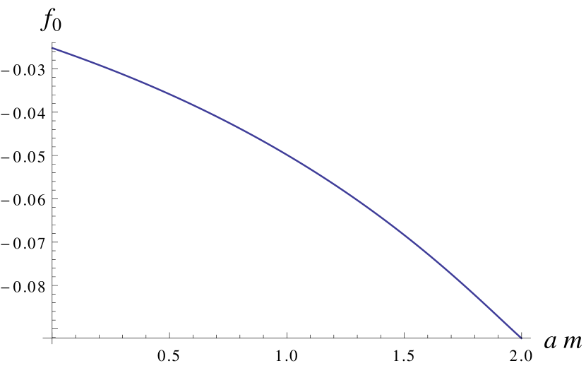
Figure 1: $f_{0}(am)$.

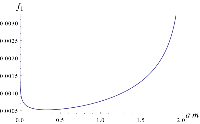
Figure 2: $f_{1}(am)$.

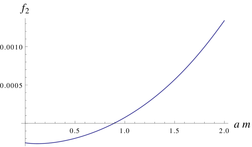
Figure 3: $f_{2}(am)$.

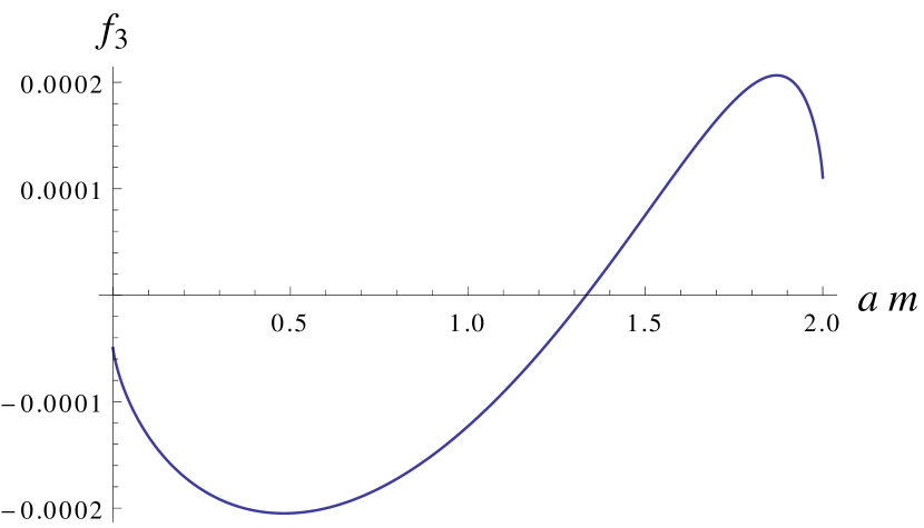
Figure 4: $f_{3}(am)$.

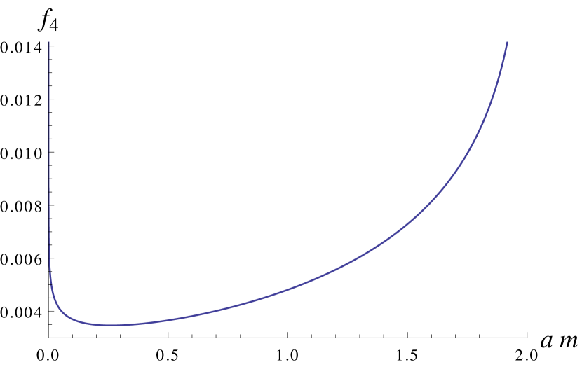
Figure 5: $f_{4}(am)$.

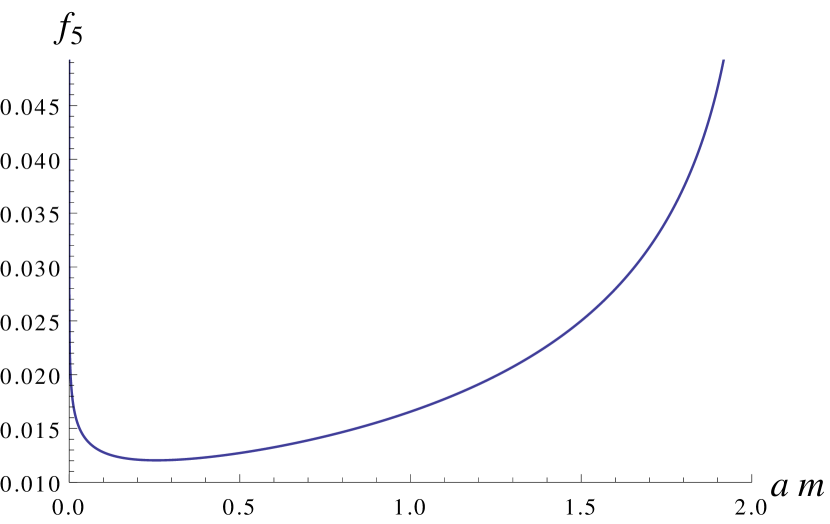
Figure 6: $f_{5}(am)$.

The continuum limit of Eq. (2.38), i.e., the parity-odd part of $\mathcal{L}(A,A_{\star};\delta A,\delta_{\star}A_{\star})$, recalling Eq. (2.23), is given by (omitting the symbol $\operatorname{tr}$),

$$\left.\mathcal{L}(A,A_{\star};\delta A,\delta_{\star}A_{\star})\right|_{\text{parity-odd}}$$

$$=-\frac{1}{32\pi^{2}}\epsilon_{\mu\nu\rho\sigma}\biggl{[}\left(\bar{F}_{\mu\nu}+\frac{1}{12}[C_{\mu},C_{\nu}]\right)\{\delta A_{\rho},\delta_{\star}A_{\star\sigma}\}$$

$$\qquad\qquad\qquad\qquad{}-\frac{1}{3}C_{\mu}(\{\delta A_{\nu},\bar{D}_{\rho}\delta_{\star}A_{\star\sigma}\}+\{\delta_{\star}A_{\star\nu},\bar{D}_{\rho}\delta A_{\sigma}\})+\frac{1}{3}\partial_{\mu}(C_{\nu}[\delta A_{\rho},\delta_{\star}A_{\star\sigma}])\biggr{]}.$$ (2.55)

Naturally, this parity-odd part is controlled by the gauge anomaly; it can be confirmed that this combination vanishes when the gauge representation of the fermion is anomaly free.

For the parity-even part (2.39), we have Lorentz symmetry-violating terms as well as Lorentz-preserving terms. For the latter, we have (again omitting the symbol $\operatorname{tr}$),

$$\left.\mathcal{L}(A,A_{\star};\delta A,\delta_{\star}A_{\star})\right|_{\text{parity-even, Lorentz-preserving}}$$

$$=\frac{f_{0}}{a^{2}}\delta A_{\mu}\delta_{\star}A_{\star\mu}$$

$$\qquad{}+\left(-\frac{3f_{1}}{2}+\frac{f_{2}}{2}-\frac{f_{3}}{2}\right)[(\bar{D}_{\mu}\delta A_{\mu})C_{\nu}\delta_{\star}A_{\star\nu}-C_{\mu}\delta A_{\mu}(\bar{D}_{\nu}\delta_{\star}A_{\star\nu})]$$

$$\qquad{}-\left(\frac{f_{1}}{2}+\frac{f_{2}}{2}-\frac{3f_{3}}{2}\right)[C_{\mu}(\bar{D}_{\nu}\delta A_{\mu})\delta_{\star}A_{\star\nu}-\delta A_{\mu}C_{\nu}(\bar{D}_{\mu}\delta_{\star}A_{\star\nu})]$$

$$\qquad{}-\left(\frac{f_{1}}{2}+\frac{f_{2}}{2}-\frac{3f_{3}}{2}\right)[C_{\nu}\delta A_{\mu}(\bar{D}_{\mu}\delta_{\star}A_{\star\nu})-(\bar{D}_{\nu}\delta A_{\mu})C_{\mu}\delta_{\star}A_{\star\nu}]$$

$$\qquad{}+\left(-\frac{7f_{1}}{2}+\frac{f_{2}}{2}+\frac{f_{3}}{2}\right)[(\bar{D}_{\mu}C_{\mu})\delta A_{\nu}\delta_{\star}A_{\star\nu}-\delta A_{\nu}(\bar{D}_{\mu}C_{\mu})\delta_{\star}A_{\star\nu}]$$

$$\qquad{}-\left(\frac{3f_{1}}{2}-\frac{f_{2}}{2}+\frac{f_{3}}{2}\right)[\delta A_{\mu}C_{\mu}(\bar{D}_{\nu}\delta_{\star}A_{\star\nu})-C_{\nu}(\bar{D}_{\mu}\delta A_{\mu})\delta_{\star}A_{\star\nu}]$$

$$\qquad{}+\left(13f_{1}-3f_{2}-3f_{3}\right)(\bar{D}_{\mu}\delta A_{\mu})(\bar{D}_{\nu}\delta_{\star}A_{\star\nu})$$

$$\qquad{}+\left(9f_{1}-3f_{2}-f_{3}\right)(\bar{D}_{\mu}\delta A_{\nu})(\bar{D}_{\mu}\delta_{\star}A_{\star\nu})$$

$$\qquad{}+\left(-19f_{1}+5f_{2}+5f_{3}\right)(\bar{D}_{\nu}\delta A_{\mu})(\bar{D}_{\mu}\delta_{\star}A_{\star\nu})$$

$$\qquad{}+\left(\frac{11f_{1}}{6}-\frac{f_{2}}{6}-\frac{7f_{3}}{6}\right)C_{\mu}\delta A_{\nu}C_{\mu}\delta_{\star}A_{\star\nu}$$

$$\qquad{}+\left(-\frac{13f_{1}}{6}+\frac{11f_{2}}{6}-\frac{7f_{3}}{6}\right)(C_{\mu}\delta A_{\mu}C_{\nu}\delta_{\star}A_{\star\nu}+C_{\nu}\delta A_{\mu}C_{\mu}\delta_{\star}A_{\star\nu})$$

$$\qquad{}+\left(-\frac{5f_{1}}{12}+\frac{19f_{2}}{12}-\frac{17f_{3}}{12}\right)(C_{\nu}C_{\mu}\delta A_{\mu}\delta_{\star}A_{\star\nu}+\delta A_{\mu}C_{\mu}C_{\nu}\delta_{\star}A_{\star\nu})$$

$$\qquad{}+\left(\frac{19f_{1}}{12}-\frac{5f_{2}}{12}-\frac{5f_{3}}{12}\right)(C_{\mu}C_{\nu}\delta A_{\mu}\delta_{\star}A_{\star\nu}+\delta A_{\mu}C_{\nu}C_{\mu}\delta_{\star}A_{\star\nu})$$

$$\qquad{}+\left(-\frac{17f_{1}}{12}+\frac{19f_{2}}{12}-\frac{11f_{3}}{12}\right)(C_{\mu}C_{\mu}\delta A_{\nu}\delta_{\star}A_{\star\nu}+\delta A_{\nu}C_{\mu}C_{\mu}\delta_{\star}A_{\star\nu})$$

$$\qquad{}+\left(\frac{9f_{1}}{2}-\frac{3f_{2}}{2}-\frac{f_{3}}{2}\right)[\partial_{\mu}(C_{\mu}\delta A_{\nu}\delta_{\star}A_{\star\nu})-\partial_{\mu}(\delta A_{\nu}C_{\mu}\delta_{\star}A_{\star\nu})]$$

$$\qquad{}+\left(f_{2}-\frac{3f_{3}}{2}\right)[\partial_{\mu}(C_{\nu}\delta A_{\mu}\delta_{\star}A_{\star\nu})-\partial_{\nu}(\delta A_{\mu}C_{\mu}\delta_{\star}A_{\star\nu})]$$

$$\qquad{}-\left(4f_{1}-f_{2}-\frac{f_{3}}{2}\right)[\partial_{\nu}(C_{\mu}\delta A_{\mu}\delta_{\star}A_{\star\nu})-\partial_{\mu}(\delta A_{\mu}C_{\nu}\delta_{\star}A_{\star\nu})]$$

$$\qquad{}+(10f_{1}-2f_{2}-4f_{3})\{\partial_{\nu}[\delta A_{\mu}(\bar{D}_{\mu}\delta_{\star}A_{\star\nu})]+\partial_{\mu}[(\bar{D}_{\nu}\delta A_{\mu})\delta_{\star}A_{\star\nu}]\}$$

$$\qquad{}+(-8f_{1}+2f_{2}+f_{3})\{\partial_{\mu}[\delta A_{\mu}(\bar{D}_{\nu}\delta_{\star}A_{\star\nu})]+\partial_{\nu}[(\bar{D}_{\mu}\delta A_{\mu})\delta_{\star}A_{\star\nu}]$$

$$\qquad\qquad\qquad\qquad\qquad\qquad{}+\partial_{\mu}[\delta A_{\nu}(\bar{D}_{\mu}\delta_{\star}A_{\star\nu})]+\partial_{\mu}[(\bar{D}_{\mu}\delta A_{\nu})\delta_{\star}A_{\star\nu}]\}.$$ (2.56)

For the parity-even, Lorentz-violating part,

$$\left.\mathcal{L}(A,A_{\star};\delta A,\delta_{\star}A_{\star})\right|_{\text{parity-even, Lorentz-violating}}$$

$$=\frac{3}{2}\left(9f_{1}-f_{2}-f_{3}-\frac{f_{4}}{2}-\frac{f_{5}}{2}\right)[(\bar{D}_{\nu}C_{\nu})\delta A_{\nu}\delta_{\star}A_{\star\nu}-\delta A_{\nu}(\bar{D}_{\nu}C_{\nu})\delta_{\star}A_{\star\nu}]$$

$$\qquad{}-\left(9f_{1}-f_{2}-f_{3}-\frac{f_{4}}{2}-\frac{f_{5}}{2}\right)(\bar{D}_{\nu}\delta A_{\nu})(\bar{D}_{\nu}\delta_{\star}A_{\star\nu})$$

$$\qquad{}+\left(\frac{47f_{1}}{2}-\frac{7f_{2}}{2}-\frac{7f_{3}}{2}+\frac{f_{4}}{4}-\frac{7f_{5}}{4}\right)C_{\nu}\delta A_{\nu}C_{\nu}\delta_{\star}A_{\star\nu}$$

$$\qquad{}+\left(\frac{67f_{1}}{4}-\frac{11f_{2}}{4}-\frac{11f_{3}}{4}+\frac{5f_{4}}{8}-\frac{11f_{5}}{8}\right)(C_{\nu}C_{\nu}\delta A_{\nu}\delta_{\star}A_{\star\nu}+\delta A_{\nu}C_{\nu}C_{\nu}\delta_{\star}A_{\star\nu})$$

$$\qquad{}+\frac{1}{2}\left(9f_{1}-f_{2}-f_{3}-\frac{f_{4}}{2}-\frac{f_{5}}{2}\right)[\partial_{\nu}(\delta A_{\nu}C_{\nu}\delta_{\star}A_{\star\nu})-\partial_{\nu}(C_{\nu}\delta A_{\nu}\delta_{\star}A_{\star\nu})]$$

$$\qquad{}+2\left(9f_{1}-f_{2}-f_{3}-\frac{f_{4}}{2}-\frac{f_{5}}{2}\right)\{\partial_{\nu}[\delta A_{\nu}(\bar{D}_{\nu}\delta_{\star}A_{\star\nu})]+\partial_{\nu}[(\bar{D}_{\nu}\delta A_{\nu})\delta_{\star}A_{\star\nu}]\}.$$ (2.57)

The local functional $\mathcal{L}(A,A_{\star};\delta A,\delta A_{\star})$ in Eq. (1.3) is given by the sum of Eqs. (2.55), (2.56), and (2.57). In particular, $\mathcal{L}(A,A_{\star}=0;\delta A,\delta_{\star}^{\omega}A_{\star}|_{A_{\star}=0})$ in Eq. (1.12) is given by setting $A_{\star\mu}(x)=0$ and $\delta_{\star}A_{\star\mu}(x)=\partial_{\mu}\omega(x)$ (and thus $C_{\mu}=-A_{\mu}$, $\bar{A}_{\mu}=(1/2)A_{\mu}$, and $\bar{D}_{\mu}=\partial_{\mu}+(1/2)[A_{\mu},\cdot]$) in the above expressions. We see that $\mathcal{L}(A,A_{\star}=0;\delta A,\delta_{\star}^{\omega}A_{\star}|_{A_{\star}=0})$ does not vanish even if the gauge representation is anomaly free. For example, from the first term of Eq. (2.56),

$$\mathcal{L}(A,A_{\star}=0;\delta A,\delta_{\star}^{\omega}A_{\star}|_{A_{\star}=0})=\frac{f_{0}}{a^{2}}\operatorname{tr}\delta A_{\mu}(x)\partial_{\mu}\omega(x)+\dotsb,$$ (2.58)

and the relation (1.12) tells us that this corresponds to the mass term of the gauge field, $(f_{0}/2a^{2})\operatorname{tr}A_{\mu}(x)A_{\mu}(x)$, in the effective action $\ln\mathcal{Z}[A,0]$. Other terms in Eqs. (2.56) and (2.57) can be understood in a similar manner, as shown in Appendix A. Such gauge-breaking terms can always be removed by local counterterms (see Appendix A), but such a necessity for counterterms for restoring the gauge symmetry will be undesirable from the perspective of a non-perturbative formulation of chiral gauge theories.

Appendix A Computation of $\delta^{\omega}\ln\mathcal{Z}[A,0]$

In this appendix, we obtain the explicit form of the “gauge symmetry-breaking” $\delta^{\omega}\ln\mathcal{Z}[A,0]$ in Eq. (1.12) and confirm that the breaking can be removed by local counterterms when the gauge representation is anomaly free. We note the identity

$$\delta^{\omega}\ln\mathcal{Z}[A,0] =\int_{0}^{1}d\xi\,\frac{d}{d\xi}\left(\delta^{\omega}\ln\mathcal{Z}[A,0]\right)_{A\to\xi A}$$

$$=\int_{0}^{1}d\xi\,\left(\delta\delta^{\omega}\ln\mathcal{Z}[A,0]\right)_{A\to\xi A,\delta A\to A}$$

$$=\int d^{4}x\,\int_{0}^{1}d\xi\,\mathcal{L}(\xi A,A_{\star}=0;A,\delta_{\star}^{\omega}A_{\star}|_{A_{\star}=0}),$$ (A.1)

where we have assumed $\left(\delta^{\omega}\ln\mathcal{Z}[A,0]\right)_{A=0}=0$. Note that $\delta_{\star}^{\omega}A_{\star\mu}|_{A_{\star}=0}=\partial_{\mu}\omega$. Then using Eqs. (2.55), (2.56), and (2.57) in the above formula, we find (omitting the symbol $\int d^{4}x\,\operatorname{tr}$)

$$\left.\delta^{\omega}\ln\mathcal{Z}[A,0]\right|_{\text{parity-odd}}=\frac{1}{24\pi^{2}}\epsilon_{\mu\nu\rho\sigma}(\partial_{\mu}\omega)\left(A_{\nu}\partial_{\rho}A_{\sigma}+\frac{1}{2}A_{\nu}A_{\rho}A_{\sigma}\right),$$ (A.2)

$$\left.\delta^{\omega}\ln\mathcal{Z}[A,0]\right|_{\text{parity-even, Lorentz-preserving}}$$

$$=\frac{f_{0}}{a^{2}}(\partial_{\mu}\omega)A_{\mu}$$

$$\qquad{}+(-13f_{1}+3f_{2}+3f_{3})(\partial_{\mu}\omega)\partial_{\mu}\partial_{\nu}A_{\nu}+(10f_{1}-2f_{2}-4f_{3})(\partial_{\mu}\omega)\partial_{\nu}\partial_{\nu}A_{\mu}$$

$$\qquad\qquad{}+(-5f_{1}+f_{2}+2f_{3})(\partial_{\mu}\omega)[\partial_{\mu}A_{\nu},A_{\nu}]+(8f_{1}-2f_{2}-f_{3})(\partial_{\mu}\omega)[\partial_{\nu}A_{\nu},A_{\mu}]$$

$$\qquad\qquad\qquad{}+\frac{1}{3}(-11f_{1}+7f_{2}-2f_{3})(\partial_{\mu}\omega)(A_{\mu}A_{\nu}A_{\nu}+A_{\nu}A_{\nu}A_{\mu})$$

$$\qquad\qquad\qquad\qquad{}+\frac{1}{3}(19f_{1}-5f_{2}-5f_{3})(\partial_{\mu}\omega)A_{\nu}A_{\mu}A_{\nu},$$ (A.3)

and

$$\left.\delta^{\omega}\ln\mathcal{Z}[A,0]\right|_{\text{parity-even, Lorentz-violating}}$$

$$=\left(9f_{1}-f_{2}-f_{3}-\frac{f_{4}}{2}-\frac{f_{5}}{2}\right)(\partial_{\mu}\omega)\left(\partial_{\mu}\partial_{\mu}A_{\mu}-[\partial_{\mu}A_{\mu},A_{\mu}]\right)$$

$$\qquad{}+\frac{1}{3}\left(57f_{1}-9f_{2}-9f_{3}+\frac{3f_{4}}{2}-\frac{9f_{5}}{2}\right)(\partial_{\mu}\omega)A_{\mu}A_{\mu}A_{\mu}.$$ (A.4)

The parity-odd breaking term (A.2) is, as expected, the consistent gauge anomaly associated with a single left-handed Weyl fermion. This cannot be written as the gauge variation of a local term and vanishes if the gauge representation is anomaly free.

Concerning the parity-even breaking terms (A.3) and (A.4), it must be possible to rewrite them as the gauge variation of local terms. In fact, we can see that (again omitting the symbol $\int d^{4}x\,\operatorname{tr}$)

$$\left.\delta^{\omega}\ln\mathcal{Z}[A,0]\right|_{\text{parity-even, Lorentz-preserving}}$$

$$=\delta^{\omega}\biggl{[}\frac{f_{0}}{2a^{2}}A_{\mu}A_{\mu}$$

$$\qquad\qquad{}+\frac{1}{2}(-13f_{1}+3f_{2}+3f_{3})A_{\mu}\partial_{\mu}\partial_{\nu}A_{\nu}$$

$$\qquad\qquad\qquad{}+(5f_{1}-f_{2}-2f_{3})(A_{\mu}\partial_{\nu}\partial_{\nu}A_{\mu}-A_{\mu}A_{\nu}\partial_{\mu}A_{\nu}+A_{\mu}A_{\nu}\partial_{\nu}A_{\mu})$$

$$\qquad\qquad\qquad\qquad{}+\frac{2}{3}(f_{1}+f_{2}-2f_{3})A_{\mu}A_{\mu}A_{\nu}A_{\nu}+\frac{1}{12}(-11f_{1}+f_{2}+7f_{3})A_{\mu}A_{\nu}A_{\mu}A_{\nu}\biggr{]},$$ (A.5)

and

$$\left.\delta^{\omega}\ln\mathcal{Z}[A,0]\right|_{\text{parity-even, Lorentz-preserving}}$$

$$=\delta^{\omega}\biggl{[}\frac{1}{2}\left(9f_{1}-f_{2}-f_{3}-\frac{f_{4}}{2}-\frac{f_{5}}{2}\right)A_{\mu}\partial_{\mu}\partial_{\mu}A_{\mu}$$

$$\qquad\qquad{}+\frac{1}{12}\left(57f_{1}-9f_{2}-9f_{3}+\frac{3f_{4}}{2}-\frac{9f_{5}}{2}\right)A_{\mu}A_{\mu}A_{\mu}A_{\mu}\biggr{]}.$$ (A.6)

Thus, these breakings can be removed by local counterterms.

References

• (1) D. M. Grabowska and D. B. Kaplan, Phys. Rev. D 94, no. 11, 114504 (2016) doi:10.1103/PhysRevD.94.114504 [arXiv:1610.02151 [hep-lat]].
• (2) D. M. Grabowska and D. B. Kaplan, Phys. Rev. Lett.  116, no. 21, 211602 (2016) doi:10.1103/PhysRevLett.116.211602 [arXiv:1511.03649 [hep-lat]].
• (3) H. Fukaya, T. Onogi, S. Yamamoto and R. Yamamura, arXiv:1607.06174 [hep-th].
• (4) R. Narayanan and H. Neuberger, JHEP 0603, 064 (2006) doi:10.1088/1126-6708/2006/03/064 [hep-th/0601210].
• (5) M. Lüscher, Commun. Math. Phys.  293, 899 (2010) doi:10.1007/s00220-009-0953-7 [arXiv:0907.5491 [hep-lat]].
• (6) M. Lüscher, JHEP 1008, 071 (2010) Erratum: [JHEP 1403, 092 (2014)] doi:10.1007/JHEP08(2010)071, 10.1007/JHEP03(2014)092 [arXiv:1006.4518 [hep-lat]].
• (7) M. Lüscher and P. Weisz, JHEP 1102, 051 (2011) doi:10.1007/JHEP02(2011)051 [arXiv:1101.0963 [hep-th]].
• (8) K. i. Okumura and H. Suzuki, PTEP 2016, no. 12, 123B07 (2016) doi:10.1093/ptep/ptw167 [arXiv:1608.02217 [hep-lat]].
• (9) H. Makino and O. Morikawa, PTEP 2016, no. 12, 123B06 (2016) doi:10.1093/ptep/ptw183 [arXiv:1609.08376 [hep-lat]].
• (10) L. Alvarez-Gaume and P. H. Ginsparg, Nucl. Phys. B 243, 449 (1984). doi:10.1016/0550-3213(84)90487-5
• (11) H. Neuberger, Phys. Lett. B 417, 141 (1998) doi:10.1016/S0370-2693(97)01368-3 [hep-lat/9707022].
• (12) H. Neuberger, Phys. Lett. B 427, 353 (1998) doi:10.1016/S0370-2693(98)00355-4 [hep-lat/9801031].
• (13) P. H. Ginsparg and K. G. Wilson, Phys. Rev. D 25, 2649 (1982). doi:10.1103/PhysRevD.25.2649
• (14) M. Lüscher, Phys. Lett. B 428, 342 (1998) doi:10.1016/S0370-2693(98)00423-7 [hep-lat/9802011].
• (15) F. Niedermayer, Nucl. Phys. Proc. Suppl.  73, 105 (1999) doi:10.1016/S0920-5632(99)85011-7 [hep-lat/9810026].
• (16) K. Fujikawa, Phys. Rev. D 29, 285 (1984). doi:10.1103/PhysRevD.29.285
• (17) W. A. Bardeen and B. Zumino, Nucl. Phys. B 244, 421 (1984). doi:10.1016/0550-3213(84)90322-5
• (18) H. Banerjee, R. Banerjee and P. Mitra, Z. Phys. C 32, 445 (1986). doi:10.1007/BF01551843
• (19) K. Fujikawa and H. Suzuki, “Path integrals and quantum anomalies,” Oxford, UK: Clarendon (2004) 284 p doi:10.1093/acprof:oso/9780198529132.001.0001
• (20) H. Suzuki, Prog. Theor. Phys.  101, 1147 (1999) doi:10.1143/PTP.101.1147 [hep-lat/9901012].
• (21) M. Lüscher, Nucl. Phys. B 549, 295 (1999) doi:10.1016/S0550-3213(99)00115-7 [hep-lat/9811032].