Solution of the $\kappa$-deformed Dirac equation with vector and scalar interactions in the context of spin and pseudospin symmetries

Abstract

The deformed Dirac equation invariant under the $\kappa$-Poincaré-Hopf quantum algebra in the context of minimal and scalar couplings under spin and pseudospin symmetries limits is considered. The $\kappa$-deformed Pauli-Dirac Hamiltonian allows us to study effects of quantum deformation in a class of physical systems, such as an Zeeman-like effect, Aharonov-Bohm effect and an anomalous-like contribution to the electron magnetic moment, between others. In our analysis, we consider the motion of an electron in a uniform magnetic field and interacting with (i) a planar harmonic oscillator and (ii) a linear potential. We verify that the particular choice of a linear potential induces a Coulomb-type term in the equation of motion. Expressions for the energy eigenvalues and wave functions are determined taking into account both symmetries limits. We verify that the energies and wave functions of the particle are modified by the deformation parameter as well as by the element of spin.

I Introduction

Quantum deformations based on the $\kappa$-Poincaré-Hopf algebra constitute an important branch of research that enables us to address problems in condensed matter and high energy physics through field equations. These field equations were first presented in Ref. PLB.1992.293.344 (see also Refs. PLB.1991.264.331 ; PLB.1993.302.419 ; PLB.1993.318.613 ; PLB.1994.329.189 ; PLB.1994.334.348 ), where a new real quantum Poincaré algebra with standard real structure, obtained by contraction of $U_{q}\left(O\left(3,2\right)\right)$. The resulting algebra of this contraction is a standard real Hopf algebra and depends on a dimension-full parameter $\kappa$ instead of the real deformation parameter $q$. This algebra is defined by the following commutation relations:

$$\left[\Pi_{\nu},\Pi_{\mu}\right]=0,\;\;\mu,\nu=0,1,2,3,$$ (1)

$$\left[M_{i},\Pi_{\mu}\right]=(1-\delta_{0\mu})i\epsilon_{ijk}\Pi_{k},\;\;i,j=1,2,3,$$ (2)

$$\left[L_{i},\Pi_{\mu}\right]=i[\Pi_{i}]^{\delta_{0\mu}}[\delta_{ij}\varepsilon^{-1}\sinh\left(\varepsilon\Pi_{0}\right)]^{1-\delta_{0\mu}},$$ (3)

$$\left[M_{i},M_{j}\right]=i\epsilon_{ijk}M_{k},$$ (4)

$$\left[M_{i},L_{j}\right]=i\epsilon_{ijk}L_{k},$$ (5)

$$\left[L_{i},L_{j}\right]=-i\epsilon_{ijk}\left[M_{k}\cosh\left(\varepsilon\Pi_{0}\right)-\frac{\varepsilon^{2}}{4}\Pi_{k}\Pi_{l}M_{l}\right],$$ (6)

where $\varepsilon$ is defined by

$$\varepsilon=\kappa^{-1}=\lim_{R\rightarrow\infty}(R\ln q),$$ (7)

with $R$ being the de Sitter curvature, $\Pi_{\mu}=(\Pi_{0},\boldsymbol{\Pi})$ are the $\kappa$-deformed generators for energy and momenta. In the above commutation relations the $M_{i}$, $L_{i}$ represent the spatial rotations and deformed boosts generators, respectively. The coalgebra and antipode for the $\kappa$-deformed Poincaré algebra was established in Ref. AoP.1995.243.90 . Since then, the algebraic structure of the $\kappa$-deformed Poincaré algebra has been investigated intensively and havebecome a theoretical field of increasing interest PLB.1994.329.189 ; PLB.1994.334.348 ; CQG.2010.27.025012 ; PLB.2012.711.122 ; NPB.2001.102-103.161 ; PLB.2002.529.256 ; PRD.2011.84.085020 ; JHEP.2011.1112.080 ; EPJC.2013.73.2472 ; PRD.2009.79.045012 ; EPJC.2006.47.531 ; EPJC.2008.53.295 ; PLB.2013.719.467 ; CQG.2004.21.2179 ; JHEP.2004.2004.28 ; PLB.1995.359.339 ; PLB.1994.339.87 ; PRD.2013.87.125009 ; PRD.2012.85.045029 ; PRD.2009.80.025014 . Through the field equations from the $\kappa$-Poincaré algebra ($\kappa$-Dirac equation PLB.1993.302.419 ; PLB.1993.318.613 ; EPJC.2003.31.129 ), we can study the physical implications of the quantum deformation parameter $\kappa$ in relativistic and nonrelativistic quantum systems. In this context, we highlight the study of relativistic Landau levels PLB.1994.339.87 , the Aharonov-Bohm effect taking into account spin effects PLB.1995.359.339 , the Dirac oscillator PLB.2014.731.327 ; PLB.2014.738.44 and the integer quantum Hall effect EPL.2016.116.31002 .

When we want to study the relativistic quantum dynamics of particles with spin, we must obviously consider the presence of external fields, which include the vector and scalar fields. The inclusion of vector and scalar potentials in the Dirac equation reveals interesting properties of symmetries in nuclear theory. The first contributions in this subject revealed the existence of $SU(2)$ symmetries, which are known in the literature as pseudospin and spin symmetries AoP.1971.65.352 ; NPB.1975.98.151 . Some investigations have been made in this scenario in order to give a meaning to these symmetries. However, it was only in a work by Ginocchio, that pseudospin symmetry was revealed. He verified that pseudospin symmetry in nuclei could arise from nucleons moving in a relativistic mean field, which has an attractive scalar and repulsive vector potential nearly equal in magnitude PRL.1997.78.436 (for a more detailed description see Ref. PR.2005.414.165 ). Spin and pseudo-spin symmetries in the Dirac equation have been studied under different aspects in recent years (see Refs. JPG.1999.25.811 ; PRA.2015.92.062137 ). Some studies have been developed taking into account the exact spin and pseudospin symmetries limits to study the relativistic dynamics of physical systems interacting with a class of potentials CTP.2012.58.807 ; FBS.2013.54.1839 ; EPJA.2009.43.73 ; AMC.2010.216.545 ; PRA.2012.86.032122 ; PRC.2012.86.052201 ; AoP.2015.356.83 ; AoP.2015.362.196 .

The present work is proposed to investigate the $\kappa$-deformed Dirac equation derived in Ref. PLB.1993.318.613 in the context of minimal and scalar couplings under spin and pseudospin symmetries limits. The structure of the paper is as follows. In Sec. II, we present the $\kappa$-deformed Dirac equation with couplings from which we derive the $\kappa$-deformed Pauli-Dirac equation, by using the usual procedure that consists of squaring the $\kappa$-deformed Dirac equation. In Sec. III, we consider the equation of Pauli and establish the spin and pseudospin symmetries limits. As an application, we consider the particle interacting with an uniform magnetic field in the $z$-direction in two different physical situations: (i) particle interacting with a harmonic oscillator and (ii) particle interacting with a linear potential. We obtain expressions for the energy eigenvalues and wave functions in both limits. In Sec. IV, we present our comments and conclusions.

II The $\kappa$-deformed Dirac equation with couplings

We begin with the deformed Dirac equation invariant under the $\kappa$ -deformed Poincaré quantum algebra PLB.1993.302.419 ; PLB.1993.318.613

$$\left\{\left(\gamma_{0}p_{0}-\gamma_{i}p_{i}\right)+\frac{1}{2}\varepsilon\left[\gamma_{0}\left(p_{0}^{2}-p_{i}p_{i}\right)-Mp_{0}\right]\right\}\psi=M\psi.$$ (8)

The interactions can be performed through the following prescriptions greiner.rqm.wf :

$$p_{i} \rightarrow p_{i}-eA_{i},$$ (9)

$$E \rightarrow E-\nu\left(r\right),$$ (10)

$$M \rightarrow M+w\left(r\right).$$ (11)

As mentioned in Ref. PLB.1993.318.613 , the couplings (9)-( 11) are quite satisfactory from the point of view of the $\kappa$ -Poincaré-Hopf algebra. Indeed, there are no operator ordering problems after the gauging that would require symmetrization in Eq. (8).

As we are interested in a planar dynamics, i.e., when the third directions of the fields involved are zero, we choose the following representation for the gamma matrices NPB.1988.307.909 :

$$\gamma_{0} = \sigma_{3},$$ (12)

$$\alpha_{1} = \gamma_{0}\gamma_{1}=\sigma_{1},$$ (13)

$$\alpha_{2} = \gamma_{0}\gamma_{2}=s\sigma_{2},$$ (14)

where the parameter $s$, which has a value of twice the spin value, can be introduced to characterizing the two spin states, with $s=+1$ for spin up and $s=-1$ for spin down. In the above representation, the $\kappa$-deformed Dirac equation including the interactions can be written as

$$\left[\mathbf{\alpha}\cdot\left(\mathbf{p}-e\mathbf{A}\right)+\gamma_{0}\left(M+w\left(r\right)\right)\right]\psi-\left[E-\nu\left(r\right)\right]\psi$$

$$+\frac{\varepsilon}{2}\left[es\left(\mathbf{\sigma}\cdot\mathbf{B}\right)\psi+\gamma_{0}\left(\left(\mathbf{\alpha}\cdot\mathbf{p}\right)w\left(r\right)\right)\right]\psi$$

$$+\frac{\varepsilon}{2}\left[M\gamma_{0}\left(\mathbf{\ \alpha}\cdot\mathbf{p}\right)+\gamma_{0}w\left(r\right)\left(\mathbf{\alpha}\cdot\mathbf{p}\right)\psi-\gamma_{0}e\left(\mathbf{\alpha}\cdot\mathbf{A}\right)M\psi\right]$$

$$-\frac{\varepsilon}{2}\left[\gamma_{0}e\left(\mathbf{\alpha}\cdot\mathbf{A}\right)w\left(r\right)\psi\right]=0.$$ (15)

Let us now determine the Dirac equation in its quadratic form. This can be accomplished by applying the matrix operator AoP.1996.251.45 ; EPJC.74.3187.2014

$$\mathbf{\alpha}\cdot\left(\mathbf{p}-e\mathbf{A}\right)+\gamma_{0}\left(M+w\left(r\right)\right)+E-\nu\left(r\right)$$

$$+\frac{\varepsilon}{2}\left[\gamma_{0}w\left(r\right)\left(\mathbf{\alpha}\cdot\mathbf{p}\right)+es\left(\mathbf{\sigma}\cdot\mathbf{B}\right)+\gamma_{0}\left(\left(\mathbf{\alpha}\cdot\mathbf{p}\right)w\left(r\right)\right)\right]$$

$$+\frac{\varepsilon}{2}\left[M\gamma_{0}\left(\mathbf{\alpha}\cdot\mathbf{p}\right)-\gamma_{0}e\left(\mathbf{\alpha}\cdot\mathbf{A}\right)M-\gamma_{0}e\left(\mathbf{\alpha}\cdot\mathbf{A}\right)w\left(r\right)\right]$$ (16)

in Eq. (15). The result is the $\kappa$-deformed Dirac-Pauli equation

$$\left(\mathbf{p}-e\mathbf{A}\right)^{2}\psi+\mathbf{\alpha}\cdot\left[\mathbf{p}\nu\left(r\right)\right]\psi-\gamma_{0}\mathbf{\alpha}\cdot\left[\mathbf{p}w\left(r\right)\right]\psi$$

$$+\left[M+w\left(r\right)\right]^{2}\psi-\left[E-\nu\left(r\right)\right]^{2}\psi-es\sigma_{z}B\psi$$

$$-\frac{\varepsilon}{2}\left\{\gamma_{0}\left[\mathbf{p}^{2}w\left(r\right)\right]+\gamma_{0}\left[\left(\mathbf{\alpha}\cdot\mathbf{p}\right)w\left(r\right)\right]\left[\left(\mathbf{\alpha}\cdot\mathbf{\ p}\right)\right]\right\}\psi$$

$$+\frac{\varepsilon}{2}\left\{2is\gamma_{0}\left[\mathbf{\sigma}\cdot\left[\left(\mathbf{p}w\left(r\right)\right)\times\mathbf{p}\right]-2ise\mathbf{\sigma}\cdot\left(\mathbf{p}w\left(r\right)\right)\times\mathbf{A}\right]\right\}\psi$$

$$+\frac{\varepsilon}{2}\left\{e\gamma_{0}\left[\left(\mathbf{\alpha}\cdot\mathbf{p}\right)w\left(r\right)\right]\left[\left(\mathbf{\ \alpha}\cdot\mathbf{A}\right)\right]-w\left(r\right)\left[\left(\mathbf{\alpha}\cdot\mathbf{p}\right)w\left(r\right)\right]\right\}\psi$$

$$+\frac{\varepsilon}{2}\left\{2MesB+2w\left(r\right)esB-M\left[\left(\mathbf{\alpha}\cdot\mathbf{p}\right)w\left(r\right)\right]\right\}\psi$$

$$+\frac{\varepsilon}{2}\left\{M\gamma_{0}\left[\left(\mathbf{\alpha}\cdot\mathbf{p}\right)\nu\left(r\right)\right]+\gamma_{0}w\left(r\right)\left[\left(\mathbf{\alpha}\cdot\mathbf{p}\right)\nu\left(r\right)\right]\right\}\psi=0.$$ (17)

It can be easily verified in Eq. (17) that after considering $\varepsilon=0$, the resulting equation is the one well known in the literature (see, for example, Ref. EPJC.2015.75.321 ). In order to apply the Eq. (17) to some physical system, we need to choose a representation for the vector potential $\mathbf{A}$ and the scalar potentials $w\left(r\right)$ and $\nu\left(r\right)$. For certain particular choices of these quantities, we can study the physical implications of quantum deformation on the properties of various physical systems of interest.

For the field configuration, we consider a constant magnetic field along the $z$-direction (in cylindrical coordinates), $\mathbf{B}=B\mathbf{\hat{z}}$, which is obtained from the vector potential (in the Landau gauge) Book.1981.Landau ,

$$\mathbf{A}=\frac{Br}{2}\mathbf{\hat{\varphi}}.$$ (18)

In this configuration, Eq. (17) reads

$$X+\frac{\varepsilon}{2}Y=0,$$ (19)

with

$$X = -\frac{\partial^{2}\psi}{\partial r^{2}}-\frac{1}{r}\frac{\partial\psi}{\partial r}-\frac{1}{r^{2}}\frac{\partial^{2}\psi}{\partial\varphi^{2}}+ieB\frac{\partial\psi}{\partial\varphi}+\frac{1}{4}e^{2}B^{2}r^{2}\psi$$ (20)

$$+ \left[M+w\left(r\right)\right]^{2}\psi-\left[E-\nu\left(r\right)\right]^{2}\psi-es\sigma_{z}B\psi$$

$$+ i\left[\frac{\partial w\left(r\right)}{\partial r}\right]\gamma_{0}\alpha_{r}\psi-i\left[\frac{\partial\nu\left(r\right)}{\partial r}\right]\alpha_{r}\psi,$$

and

$$Y = \gamma_{0}\left[\frac{\partial^{2}w\left(r\right)}{\partial r^{2}}+\frac{1}{r}\frac{\partial w\left(r\right)}{\partial r}\right]\psi-\gamma_{0}\left[\frac{\partial w\left(r\right)}{\partial r}\right]\frac{\partial\psi}{\partial r}$$ (21)

$$- is\left[\frac{1}{r}\frac{\partial w\left(r\right)}{\partial r}\right]\frac{\partial\psi}{\partial\varphi}-2is\left[\frac{1}{r}\frac{\partial w\left(r\right)}{\partial r}\right]\frac{\partial\psi}{\partial\varphi}$$

$$- iw\left(r\right)\gamma_{r}\left[\frac{\partial\nu\left(r\right)}{\partial r}\right]\psi+iw\left(r\right)\alpha_{r}\left[\frac{\partial w\left(r\right)}{\partial r}\right]\psi$$

$$+ es\left[\frac{\partial w\left(r\right)}{\partial r}\right]\frac{Br}{2}\psi-2es\left[\frac{\partial w\left(r\right)}{\partial r}\right]\frac{Br}{2}\psi$$

$$- iM\gamma_{r}\left[\frac{\partial\nu\left(r\right)}{\partial r}\right]\psi+iM\alpha_{r}\left[\frac{\partial w\left(r\right)}{\partial r}\right]\psi$$

$$+ 2MesB\psi+2w\left(r\right)esB\psi$$

where the matrices (12)-(14) are now given in cylindrical coordinates, $\gamma_{r}=i\sigma_{\varphi}$, $\gamma_{\varphi}=-is\sigma_{r}$, with EPJC.2015.75.321

$$\alpha_{r} = \gamma_{0}\gamma_{r}=\left(\begin{array}[]{cc}0&e^{-is\varphi}\\ e^{is\varphi}&0\end{array}\right),$$ (24)

$$\alpha_{\varphi} = \gamma_{0}\gamma_{\varphi}=\left(\begin{array}[]{cc}0&-ie^{-is\varphi}\\ ie^{is\varphi}&0\end{array}\right),$$ (27)

$$\gamma_{0} = \sigma_{z}=\left(\begin{array}[]{cc}1&0\\ 0&-1\end{array}\right).$$ (30)

We will attribute expressions to functions $\nu\left(r\right)$ and $w\left(r\right)$ in Eq. (19) in the next section, when we treat analysis of spin and pseudo-spin symmetries. We will argue after that only some particular choices for these functions will lead to a differential equation that admits an exact solution.

III Symmetries limits

To implement the spin and pseudospin symmetries limits, we make in Eq. (19) the requirement that $w\left(r\right)=\pm\nu\left(r\right)$, where the plus(minus) signal refers to spin(pseudo-spin) symmetry, respectively PRL.1997.78.436 . Next, by using $\psi=\left(\psi_{+},\psi_{-}\right)^{T}$, the first and second lines in Eq. (19) can be written in a simple form, which allows us to solve them separately. Furthermore, as mentioned above, we need to choose a representation for the radial function $\nu\left(r\right)$. We give a representation in terms of cylindrically symmetric scalar potentials which lead to results well-known in the literature.

III.1 Particle interacting with a harmonic oscillator

Because of applications to various physical systems, we consider the potential of a harmonic oscillator, $\nu\left(r\right)=\pm w\left(r\right)=ar^{2}$, where $a$ is a constant. For the Eq. (19), one can check that the spin symmetry is sufficient to decouple the radial equation that comes from the upper spinor component while the pseudo-spin symmetry decouples the radial equation that comes from the lower component of the spinor. Thus, by adopting solutions of the form

$$\psi_{\pm}=\left(\begin{array}[]{c}\sum_{m}f_{+}\left(r\right)e^{im\varphi}\\ i\sum_{m}f_{-}\left(r\right)e^{i\left(m+s\right)\varphi}\end{array}\right),$$ (31)

we arrive at radial equations

$$\frac{d^{2}f_{\pm}(r)}{dr^{2}} +\left(\frac{1}{r}+\varepsilon ar\right)\frac{df_{\pm}(r)}{dr}-\frac{\left(m^{\pm}\right)^{2}}{r^{2}}f_{\pm}(r)$$ (32)

$$-\left(\omega^{\pm}\right)^{2}r^{2}f_{+}(r)+k^{\pm}f_{+}(r)=0,$$

where $k^{+}=E^{2}-M^{2}+2\left(m+s\right)\omega-\varepsilon\left(2a+3sma+2M\omega s\right)$, $k^{-}=E^{2}-M^{2}+2\omega\left(m+s\right)+2\omega s-\varepsilon\left[2a-3sa\left(m+s\right)+2M\omega s\right]$, $\left[\omega^{+}\right]^{2}=\omega^{2}+2\left(M+E\right)a-\varepsilon\omega sa$, $\left[\omega^{-}\right]^{2}=\omega^{2}+2\left(E-M\right)a-\varepsilon\omega sa$, $\omega=eB/2$, $m^{+}=m$ and $m^{-}=m+s$. It is convenient to write Eq. (32) in a known canonical form. This can be accomplished using $f_{\pm}(r)$ as

$$f_{\pm}(\rho)=e^{-\frac{1}{2}\left(\kappa^{\pm}+1\right)\rho}\rho^{\frac{1}{2}\left|m^{\pm}\right|}F_{\pm}\left(\rho\right),\;\;\rho=\omega^{\pm}r^{2}$$ (33)

where $\kappa^{\pm}=\varepsilon a/2\omega^{\pm}$, which leads to the equation

$$\rho\frac{d^{2}F_{\pm}}{d\rho^{2}} + \left(1+\left|m^{\pm}\right|-\rho\right)\frac{dF_{\pm}}{d\rho}$$ (34)

$$- \left[\frac{1}{2}\left(1+\left|m^{\pm}\right|+\kappa^{\pm}\right)-\frac{k^{\pm}}{4\omega^{+}}\right]F_{\pm}=0.$$

Equation (34) is of the confluent hypergeometric equation type and its solution is given in terms of the Kummer functions. In this manner, the general solution for Eq. (32) is given by Book.2010.NIST

$$f_{\pm}(\rho)=\mathit{c}_{1}\,e^{-\frac{1}{2}\left(1+\kappa^{\pm}\right)\rho}\rho^{\frac{1}{2}\left|m^{\pm}\right|}$$

$$\times\,{\mathrm{M}\left(\frac{1}{2}\left(1+\left|m^{\pm}\right|+\kappa^{\pm}\right)-\frac{k^{\pm}}{4\omega^{\pm}},1+\left|m^{\pm}\right|,\rho\right)}$$

$$+\,\mathit{c}_{2}\,{e^{-\frac{1}{2}\left(1+\kappa^{\pm}\right)\rho}\rho^{-\frac{1}{2}\left|m^{\pm}\right|}}$$

$$\times\,{{\mathrm{M}\left(\frac{1}{2}\left(1-\left|m^{\pm}\right|+\kappa^{\pm}\right)-\frac{k^{\pm}}{4\omega^{\pm}},1-\left|m^{\pm}\right|,\rho\right),}}$$ (35)

where $\mathrm{M}$ are the Kummer functions. In particular, when $\left(1+\left|m^{\pm}\right|+\kappa^{\pm}\right)/2-k^{\pm}/4\omega^{\pm}=-n$, with $n=0,1,2,...$, the function $\mathrm{M}$ becomes a polynomial in $\rho$ of degree not exceeding $n$. From this condition, we extract the energies for the spin and pseudospin symmetries limits, given respectively by

$$E^{2} -M^{2}=2\sqrt{\omega^{2}+2\left(M+E\right)a-\varepsilon\omega sa}$$

$$\times\left(2n+\left|m\right|+1\right)+\varepsilon\left(3a+3sma+2\omega Ms\right)$$

$$-2\omega\left(m+s\right),$$ (36)

$$E^{2} -M^{2}=2\sqrt{\omega^{2}+2\left(E-M\right)a+\varepsilon\omega sa}$$

$$\times\left(2n+1+\left|m+s\right|\right)-2\omega\left(m+s\right)-2\omega s$$

$$-\varepsilon\left[a-3sa\left(m+s\right)+2M\omega s\right].$$ (37)

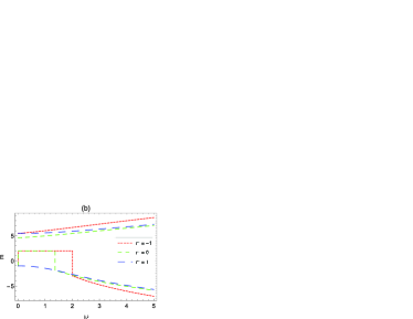
Figure 1: (Color online) Illustration of the energy eigenvalues in the spin symmetry limit (Eq. (36)) as a function of the parameter $\omega$ for (a) $s=1$ and (b) $s=-1$. We use units such as $M=1$, $n=1$, $a=1$ and an upper bound $\varepsilon=10^{-7}$.

Figure 2: (Color online) Illustration of the energy eigenvalues in the pseudospin symmetry limit (Eq. (37)) as a function of the parameter $\omega$ for (a) $s=1$ and (b) $s=-1$. We use units such as $M=1$, $n=1$, $a=1$ and an upper bound $\varepsilon=10^{-7}$.

Equations (36) and (37) are, respectively, the particle and antiparticle energies in the context of quantum deformation and they can be read as a relativistic generalization of the Landau levels. It must be emphasized that, since $\varepsilon$ and $a$ are positive, the quantum deformation affects the separation of the energy levels of the system. This feature, however, should not depend on the value of the spin projection parameter $s$. Figure 1 shows the energy profile (36) as a function of the frequency $\omega$ for some values of the quantum number $m$. In Fig. 1(a), we plotted for $s=1$ and in the Fig. 1(b) for $s=-1$. In this analysis as well as for the others we use $\varepsilon=10^{-7}$ PLB.2013.719.467 ; EPL.2016.116.31002 . For this value, the effects of quantum deformation become more evident. We clearly see that both particle and antiparticle belong to the same energy spectrum. However, in Fig. 1(b), we find that the antiparticle energy is not defined in the frequency ranges $0<\omega<1.37$ (for $m=0$) and $0<\omega<2.0$ (for $m=-1$). These same characteristics are also present in the energy profile of the Eq. (37) as shown in Fig. 2. However, in Fig. 2(b), the energies are not defined in the frequency ranges $0<\omega<3.35$ (for $m=-1$), $0<\omega<3.1$ (for $m=-1$) and $0<\omega<2.65$ (for $m=1$). The appearance of such regions characterizing the absence of energy eigenvalues is due to the quantum deformation effects present in the model. In fact, when $\varepsilon=0$, we obtain the energy eigenvalues of Ref. EPJC.2015.75.321 (after removing the magnetic flux parameter), which shows the consistency of the model in question. In particular, when $a$ and $\varepsilon$ are null, we obtain

$$E^{2}-M^{2} =2\omega\left[2n+1+\left|m\right|-m-s\right],$$ (38)

$$E^{2}-M^{2} =2\omega\left[2n+1+\left|m+s\right|-\left(m+s\right)-s\right],$$ (39)

which are the usual relativistic Landau levels with the inclusion of the element of spin.

III.2 Particle interacting with a linear potential

Let us consider the case where the particle interacts with a linear potential, $br$. In this case, we make $\nu\left(r\right)=\pm w\left(r\right)=br$ (where $b$ is a constant) in Eq. (19) to the limits of spin and pseudo-spin symmetries and proceed as before. The resulting equation is given by

$$\left[\frac{d^{2}}{dr^{2}}+\left(\frac{1}{r}+\frac{\varepsilon b}{2}\right)\frac{d}{dr}-\frac{\left(m^{\pm}\right)^{2}}{r^{2}}-\omega^{2}r^{2}-\mu^{\pm}r\right]f_{\pm}\left(r\right)$$

$$-\left(\frac{k^{\pm}}{r}-l^{\pm}\right)f_{\pm}\left(r\right)=0,$$ (40)

with $m^{+}=m$, $m^{-}=m+s$, $\mu^{+}=2\left(E+M\right)b+3\varepsilon\omega bs/2$, $\mu^{-}=2\left(E-M\right)b-3\varepsilon\omega bs/2$, $k^{+}=\varepsilon b\left(1+3sm\right)/2$, $k^{-}=\varepsilon b\left[1-3s\left(m+s\right)\right]/2$, $l^{+}=E^{2}-M^{2}+2\omega\left(m+s\right)-2M\varepsilon\omega s$ and $l^{-}=E^{2}-M^{2}+2\omega\left(m+s\right)+2\omega s\left(1-\varepsilon M\right)$. In Eq. (40), the $+(-)$ sing refer to spin and pseudo-spin symmetries, respectively. By performing the variable change, $x=\sqrt{\omega}r$, Eq. (40) assumes the form

$$\left[\frac{d^{2}}{dx^{2}}+\left(\frac{1}{x}+\frac{\kappa}{2}\right)\frac{d}{dx}-\frac{\left(m^{\pm}\right)^{2}}{x^{2}}-x^{2}-a_{L}^{\pm}x\right]f_{\pm}\left(x\right)$$

$$-\left(\frac{a_{C}^{\pm}}{x}-\frac{l^{\pm}}{\omega}\right)f_{\pm}\left(x\right)=0,$$ (41)

where we have defined the parameters $\kappa=\varepsilon b/\sqrt{\omega}$, $a_{L}^{\pm}=\mu^{\pm}/\omega\sqrt{\omega}$ e $a_{C}^{\pm}=k^{\pm}/\sqrt{\omega}$. Note that the choice $\nu\left(r\right)=br$ induces a Coulomb-like interaction in the resulting deformed sector of the eigenvalue equation. The origin of this Coulomb potential is due purely to the quantum deformation and boundary symmetries involved.

Equation (41) is of the Heun equation type, which is a homogeneous, linear, second-order, differential equation defined in the complex plane. This equation can be put into its canonical form using the solution

$$f_{\pm}\left(x\right)={x}^{\left|m^{\pm}\right|}e{{}^{-\frac{1}{2}{x}^{2}}}e{{}^{-\frac{1}{2}\left(a_{L}^{\pm}+\frac{1}{2}\kappa\right)x}y}_{\pm}\left(x\right),$$ (42)

where ${y}_{\pm}$ satisfies the biconfluent Heun differential equation

$${y}_{\pm}^{{}^{\prime\prime}} +\left(\frac{\alpha^{\pm}+1}{x}-2{x}-\beta^{\pm}\right){y}_{\pm}^{\prime}+\left(\gamma^{\pm}-\alpha^{\pm}-{2}\right)y_{\pm}$$

$$-\frac{1}{2x}\left[{\beta^{\pm}}\left(\alpha^{\pm}+{1}\right)+\delta^{\pm}\right]y_{\pm}=0,$$ (43)

with $\alpha^{\pm}=2{\left|m^{\pm}\right|}$, $\beta^{\pm}=a_{L}^{\pm}$, $\gamma^{\pm}=\left(\beta^{\pm}\right)^{2}/4+l^{\pm}/\omega$ and $\leavevmode\nobreak\ \delta^{\pm}={\kappa/2}+2a_{C}^{\pm}$. Equation (43) has a regular singularity at $x=0$, and an irregular singularity at $\infty$ of rank $2$. Usually, the solution of this equation is given in terms of two linearly independent solutions as

$$y_{\pm}\left(x\right) = \mathit{N}\left(\alpha^{\pm},\beta^{\pm},\gamma^{\pm},\delta^{\pm};x\right)$$ (44)

$$+ {x}^{-\alpha^{\pm}}\mathit{N}\left(-\alpha^{\pm},\beta^{\pm},\gamma^{\pm},\delta^{\pm};x\right),$$

where (assuming that $\alpha^{\pm}$ is not a negative integer)

$$\mathit{N}\left(\alpha^{\pm},\beta^{\pm},\gamma^{\pm},\delta^{\pm};x\right)=\sum\limits_{q=0}^{\infty}\frac{{\mathcal{A}}_{q}^{\pm}\left(\alpha^{\pm},\beta^{\pm},\gamma^{\pm},\delta^{\pm}\right)}{\left(1+\alpha^{\pm}\right)_{q}}\frac{x^{q}}{q!}$$ (45)

are the Heun functions. After the insertion of this solution into Eq. (43), we find ($q\geqslant 0$)

$$\mathcal{A}_{0}=1,$$ (46)

$$\mathcal{A}_{1}^{\pm}=\frac{1}{2}\left[\delta^{\pm}+\beta^{\pm}\left(1+\alpha^{\pm}\right)\right],$$ (47)

$$\mathcal{A}_{q+2}^{\pm}=\left\{\left(q+1\right)\beta^{\pm}+\frac{1}{2}\left[\delta^{\pm}+\beta^{\pm}\left(1+\alpha^{\pm}\right)\right]\right\}\mathcal{A}_{q+1}^{\pm}$$

$$-\left(q+1\right)\left(q+1+\alpha^{\pm}\right)\left[\gamma^{\pm}-\alpha^{\pm}-2-2q\right]\mathcal{A}_{q}^{\pm},$$ (48)

where

$$\left(1+\alpha^{\pm}\right)_{q}=\frac{\Gamma\left(q+\alpha^{\pm}+1\right)}{\Gamma\left(\alpha^{\pm}+1\right)},\;\;q=0,1,2,3,\ldots.$$ (49)

From the recursion relation (48), the function $N\left(\alpha^{\pm},\beta^{\pm},\gamma^{\pm},\delta^{\pm};x\right)$ becomes a polynomial of degree $n$ if and only if the two following conditions are imposed:

$$\gamma^{\pm}-\alpha^{\pm}-2=2n,\;\;n=0,1,2,\ldots$$ (50)

$$\mathcal{A}_{n+1}^{\pm}=0,$$ (51)

where $n$ is a positive integer. In this case, the $\left(n+1\right)$th coefficient in the series expansion is a polynomial of degree $n$ in $\delta^{\pm}$. When $\delta^{\pm}$ is a root of this polynomial, the $\left(n+1\right)$th and subsequent coefficients cancel and the series truncates, resulting in a polynomial form of degree $n$ for $N\left(\alpha^{\pm},\beta^{\pm},\gamma^{\pm},\delta^{\pm};x\right)$. From condition (50), we extract the energies at the spin and pseudo symmetries limit, given respectively by

$$E_{nm}^{2}-M^{2}=2\omega_{nm}\left({n}+{\left|m\right|+1}\right)-\frac{b^{2}}{\omega_{nm}^{2}}\left(E_{nm}+M\right)^{2}$$

$$-\frac{3b^{2}}{2\omega_{nm}}\left(E_{nm}+M\right)\varepsilon s+2\omega_{nm}\left[\varepsilon Ms-\left(m+s\right)\right],$$ (52)

$$E_{nm}^{2}-M^{2}=2\omega_{nm}\left({n}+{\left|m+s\right|+1}\right)-\frac{b^{2}}{\omega_{nm}^{2}}\left(E_{nm}-M\right)^{2}$$

$$+\frac{3b^{2}}{2\omega_{nm}}\left(E_{nm}-M\right)\varepsilon s-2\omega_{nm}\left[s\left(1-\varepsilon M\right)+\left(m+s\right)\right].$$ (53)

The energy of a physical system must be a function involving all the parameters present in the equation of motion. In Eqs. (52) and (53) the parameter $a_{C}^{\pm}$ is absent. However, it can be restored using the condition (51) from which we obtain a relation between such parameter and the frequency of the system. For each value of $n$ fixed, we have a self-energy and its corresponding wave function. Let us consider the solution (45) up to second-order in $x$ of the expansion,

$$N\left(\alpha^{\pm},\beta^{\pm},\gamma^{\pm},\delta^{\pm};x\right) = \frac{\mathcal{A}_{0}}{\left(1+\alpha^{\pm}\right)_{0}}+\frac{\mathcal{A}_{1}^{\pm}}{\left(1+\alpha^{\pm}\right)_{1}}x$$ (54)

$$+ \frac{\mathcal{A}_{2}^{\pm}}{\left(1+\alpha^{\pm}\right)_{2}}\frac{x^{2}}{2!}+\ldots.$$

If we truncate the series in a term of order $x^{n}$, the resulting finite series is related, via solution (42), to the energy level $E_{n}$. Thus, the physical quantity that we can associate most closely with the series (54) truncated in the term $x^{n}$ is the energy $E_{n}$ of the particle with the wave function (42). In fact, it is necessary that the series (54) becomes a $n$-degree polynomial for the system to admit bound states. Thus, by using the relation (48) and Eqs. (46)-(47), the coefficient above $\mathcal{A}_{2}^{\pm}$ can be determined. If we want to truncate solution (54) in $x$, we must impose that $A_{1}^{\pm}=0$ through the condition (51); when we truncate in $x^{2}$, we make $A_{2}^{\pm}=0$, and so on. For each of these cases, we can establish a appropriate constraints between conditions (50) and (51). Since the Eqs. (52)-(53) are of the relativistic Landau level type, we prefer to fix the frequency $\omega$ in order to obtain an expression for the energies corresponding to each value of $n$. For this, we rewrite the frequency $\omega$ as $\omega^{\pm}$, with $\pm$ labelling spin and pseudo-spin as above. After obtaining $\omega_{nm}^{\pm}$ and replace them in Eqs. (52)-(53), we will have expressions for the energies involving the quantities $\alpha^{\pm}$, $\beta^{\pm}$, $\gamma^{\pm}$, $\delta^{\pm}$, which contains the coupling constant $a_{C}^{\pm}$, the mass of the particle $M$ and the quantum angular momentum number $m^{\pm}$. Thus, for $A_{1}^{\pm}=0$, it means that we are investigating the particular solution for $n=0$. In this case, from Eq. (47), we have

$$\frac{1}{2}\left(\delta^{\pm}+\beta^{\pm}\tilde{m}^{\pm}\right)=0,$$ (55)

where $\tilde{m}^{\pm}=1+\alpha^{\pm}$. Solving (55) for $\omega$, we get the relations

$$\omega_{0m}^{+} = -\frac{2\left(E_{0m}^{+}+M\right)\left(1+2{\left|m\right|}\right)}{\varepsilon\left[3s\left({\left|m\right|}+m\right)+\frac{3}{2}\left(s+{1}\right)\right]},$$ (56)

$$\omega_{0m}^{-} = \frac{2\left(E_{0m}^{-}-M\right)\left(1+2{\left|m+s\right|}\right)}{\varepsilon\left[3s\left({\left|m+s\right|}+m+s\right)+\frac{3}{2}\left(s-{1}\right)\right]}.$$ (57)

Proceeding in a similar way to $\mathcal{A}_{2}^{\pm}=0$, we find the following third degree polynomial in $\omega_{1m}^{\pm}$ ($n=1$):

$$\mathcal{A}^{\pm}\left[\omega_{1m}^{\pm}\right]^{3}+\mathcal{B}^{\pm}\left[\omega_{1m}^{\pm}\right]^{2}+\mathcal{C}^{\pm}\left[\omega_{1m}^{\pm}\right]+\mathcal{D}^{\pm}=0,$$ (58)

with

$$\mathcal{A}^{+}=2\left(1+2{\left|m\right|}\right),$$

$$\mathcal{A}^{-}=2\left(1+2{\left|m+s\right|}\right),$$

$$\mathcal{B}^{+}=\mathcal{B}^{-}=0,$$

$$\mathcal{C}^{+}=-\frac{3}{2}\varepsilon b^{2}\left(E_{1m}^{+}+M\right)\Big{[}\left(2\left|m\right|+1\right)s+C^{+}\Big{]},$$

$$\mathcal{C}^{-}=\frac{3}{2}\varepsilon b^{2}\left(E_{1m}^{-}-M\right)\Big{[}s\left(2\left|m+s\right|+1\right)+C^{-}\Big{]},$$

$$\mathcal{D}^{+}=-b^{2}\left(E_{1m}^{+}+M\right)^{2}\left(1+2{\left|m\right|}\right)\left(3+2{\left|m\right|}\right),$$

$$\mathcal{D}^{-}=-b^{2}\left(E_{1m}^{-}-M\right)^{2}\left(1+2{\left|m+s\right|}\right)\left(3+2{\left|m+s\right|}\right),$$

where $C^{+}=2\left(1+\left|m\right|\right)\left(2s\left|m\right|+2ms+s+1\right)$ and $C^{-}=2\left(\left|m+s\right|+1\right)\left(2s\left(\left|m+s\right|+m\right)+s+1\right)$. Equation (58) has only one real root. For each specific frequency, $\omega_{0m}^{\pm}$, $\omega_{1m}^{\pm}$, we can determine the energies $E_{0m}^{\pm}$ and $E_{1m}^{\pm}$ by the following expressions:

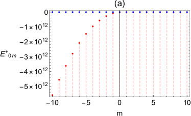
Figure 3: (Color online) Illustration of the energy eigenvalues in the spin symmetry limit (Eq. (59)) as a function of the parameter $\omega$ for (a) $s=1$ and (b) $s=-1$. We use units such as $M=1$, $n=1$, $b=1$ and $\varepsilon=10^{-7}$.

Figure 4: (Color online) Illustration of the energy eigenvalues in the pseudospin symmetry limit (Eq. (60)) as a function of the parameter $\omega$ for (a) $s=1$ and (b) $s=-1$. We use units such as $M=1$, $n=1$, $b=1$ and $\varepsilon=10^{-7}$.

$$\left(E_{0m}^{+}\right)^{2} -M^{2}=2\omega_{0m}^{+}\left({\left|m\right|+1}\right)$$

$$-\frac{b^{2}}{\left(\omega_{0m}^{+}\right)^{2}}\left(E_{0m}^{+}+M\right)^{2}-\frac{3b^{2}}{2\omega_{0m}^{+}}\left(E_{0m}^{+}+M\right)\varepsilon s,$$ (59)

$$\left(E_{0m}^{-}\right)^{2} -M^{2}=2\omega_{0m}^{-}\left({\left|m+s\right|+1}\right)$$

$$-\frac{b^{2}}{\left(\omega_{0m}^{-}\right)^{2}}\left(E_{0m}^{-}-M\right)^{2}+\frac{3b^{2}}{2\omega_{0m}^{-}}\left(E_{0m}^{-}-M\right)\varepsilon s$$

$$-2\omega_{0m}^{-}\left[s\left(1-\varepsilon M\right)+\left(m+s\right)\right]$$ (60)

and

$$\left(E_{1m}^{+}\right)^{2} -M^{2}=2\omega_{1m}^{+}\left({\left|m\right|+2}\right)$$

$$-\frac{b^{2}}{\left(\omega_{1m}^{+}\right)^{2}}\left(E_{1m}^{+}+M\right)^{2}-\frac{3b^{2}}{2\omega_{1m}^{+}}\left(E_{1m}^{+}+M\right)\varepsilon s$$

$$+2\omega_{1m}^{+}\left[\varepsilon Ms-\left(m+s\right)\right],$$ (61)

$$\left(E_{1m}^{-}\right)^{2} -M^{2}=2\omega_{1m}^{-}\left({\left|m+s\right|+2}\right)$$

$$-\frac{b^{2}}{\left(\omega_{1m}^{-}\right)^{2}}\left(E_{1m}^{-}-M\right)^{2}+\frac{3b^{2}}{2\omega_{1m}^{-}}\left(E_{1m}^{-}-M\right)\varepsilon s$$

$$-2\omega_{1m}^{-}\left[s\left(1-\varepsilon M\right)+\left(m+s\right)\right],$$ (62)

where $\omega_{1m}^{\pm}$ is given by

$$\omega_{1m}^{\pm}=\sqrt[3]{\frac{\Delta^{\pm}}{18}}\frac{1}{\mathcal{A}^{\pm}}-\sqrt[3]{\frac{2}{3\Delta^{\pm}}}\mathcal{C}^{\pm},$$ (63)

with

$$\Delta^{\pm}=\sqrt{3}\sqrt{27\left[\mathcal{A}^{\pm}\right]^{4}\left[\mathcal{D}^{\pm}\right]^{2}+4\left[\mathcal{A}^{\pm}\right]^{3}\left[\mathcal{C}^{\pm}\right]^{3}}-9\left[\mathcal{A}^{\pm}\right]^{2}\mathcal{D}^{\pm}.$$ (64)

Such energies represent the first two energy levels of the system. For simplicity, we perform a numerical analysis only for the case $n=0$. In this way, by studying the Eq. (59), we find that for $s=1$ and $m>0$, the energy of the particle is infinitely degenerate, with respective eigenvalues $E_{0m}^{+}=-1$ and $E_{0m}^{+}=-0.33$ whereas for $m<0$, only one of the roots is infinitely degenerate with energy $E_{0m}^{+}=-1$ (Fig. 3(a)). On the other hand, when we analyze the Eq. (59) for $s=-1$, we verify that the energy spectrum is defined only for $m>0$, and one of the roots is infinitely degenerate with eigenvalue $E_{0m}^{+}=-1$ (Fig. 3(b)). These characteristics are also present in the energies from Eq. (60). For $s=1$, the energies are defined only for $m>0$ and one of the roots is infinitely degenerate, with eigenvalue $E_{0m}^{-}=1$ (Fig. 4(a)). For $s=-1$ and $m<0$, there is an infinitely degenerate root with eigenvalue $E_{0m}^{-}=1$ while for $m>0$ both roots are infinitely degenerate with respective energies $E_{0m}^{-}=1$ and $E_{0m}^{-}=-2.7\times 10^{7}$ (Fig. 4(b)).

Finally, to determine the energies corresponding to $n=2,3,4,\ldots$, we must make use of the above recipe. However, as we can see from Eq. (58), the polynomials of degree $n\geq 3$ resulting from condition (51), in general, not all roots are physically acceptable.

IV Conclusions

We have studied the relativistic quantum dynamics of a spin-$1/2$ charged particle with minimal, vector and scalar couplings in the quantum deformed framework generated by the $\kappa$-Poincaré-Hopf algebra. The problem have been formulated using the $\kappa$-deformed Dirac equation in two dimensions. The $\kappa$-deformed Pauli equation was derived to study the dynamics of the system taking into account the spin and pseudospin symmetries limits. For the $\kappa$-deformed Dirac-Pauli equation obtained (Eq. (19)), we have argued that only particular choices of radial function $\nu\left(r\right)$ lead to exactly solvable differential equations. We have considered the case where the particle interacts with an uniform magnetic field, a planar harmonic oscillator and a linear potential. We have verified that the linear potential leads to a Coulomb-type term in the $\kappa$-deformed sector of the radial equation. The resulting equation obtained is a Heun-type differential equation. Analytical solutions for both spin and pseudospin symmetries limits enabled us to obtain expressions for the energy eigenvalues (through the use of the Eqs. (50) and (51)) and wave functions. Because of the limitations imposed by the condition (51), we have derived expressions for the energies corresponding only to $n=0$ (Eqs. (59)-(60)) and $n=1$ (Eqs. (61)-(62)). We have shown that the energy eigenvalues and wave functions are modified by both the spin element $s$ and the deformation parameter $\varepsilon$. We believe that future experiments may provide some estimate on the magnitude of the deformation parameter within the context of the model studied.

References

• (1) Jerzy Lukierski, Anatol Nowicki and Ruegg H 1992 Phys. Lett. B 293 344 ISSN 0370-2693
• (2) Lukierski J, Ruegg H, Nowicki A and Tolstoy V N 1991 Phys. Lett. B 264 331 ISSN 0370-2693
• (3) Anatol Nowicki, Emanuele Sorace and Marco Tarlini 1993 Phys. Lett. B 302 419–422 ISSN 0370-2693
• (4) L C Biedenharn, Berndt Mueller and Marco Tarlini 1993 Phys. Lett. B 318 613–616 ISSN 0370-2693
• (5) Jerzy Lukierski and Henri Ruegg 1994 Phys. Lett. B 329 189 ISSN 0370-2693
• (6) Majid S and Ruegg H 1994 Phys. Lett. B 334 348 ISSN 0370-2693
• (7) Lukierski J, Ruegg H and Zakrzewski W 1995 Ann. Phys. (NY) 243 90 ISSN 0003-4916
• (8) Michele Arzano, Jerzy Kowalski-Glikman and Adrian Walkus 2010 Classical and Quantum Gravity 27 025012
• (9) Kovacević D, Meljanac S, Pachoł A and Štrajn R 2012 Physics Letters B 711 122 ISSN 0370-2693
• (10) Kosiński P, Lukierski J and Maślanka P 2001 Nucl. Phys. B - Proc. suppl. 102-103 161 ISSN 0920-5632
• (11) M V Cougo-Pinto, C Farina and J F M Mendes 2002 Phys. Lett. B 529 256 ISSN 0370-2693
• (12) Harikumar E, Jurić T and Meljanac S 2011 Phys. Rev. D 84(8) 085020
• (13) Marija Dimitrijević and Larisa Jonke 2011 Journal of High Energy Physics 1112 080
• (14) Tajron Jurić, Stjepan Meljanac and Rina Štrajn 2013 Eur. Phys. J. C 73 2472 ISSN 1434-6044
• (15) Borowiec A and Pachol A 2009 Phys. Rev. D 79(4) 045012
• (16) Meljanac S and Stojić M 2006 Eur. Phys. J. C 47 531 ISSN 1434-6044
• (17) Meljanac S, Samsarov A, Stojić M and Gupta K S 2008 Eur. Phys. J. C 53 295 ISSN 1434-6044
• (18) Andrade F M and Silva E O 2013 Phys. Lett. B 719 467 ISSN 0370-2693
• (19) Alessandra Agostini, Giovanni Amelino-Camelia and Michele Arzano 2004 Class. Quantum Grav. 21 2179
• (20) Roberto Aloisio, Angelo Galante, Aurelio F Grillo, Fernando Méndez, José M Carmona and José L Cortés 2004 J. High Energy Phys. 2004 028
• (21) Roy P and Roychoudhury R 1995 Phys. Lett. B 359 339 ISSN 0370-2693
• (22) Roy P and Roychoudhury R 1994 Phys. Lett. B 339 87 ISSN 0370-2693
• (23) Meljanac S, Pachoł A, Samsarov A and Gupta K S 2013 Phys. Rev. D 87(12) 125009
• (24) Gupta K S, Meljanac S and Samsarov A 2012 Phys. Rev. D 85(4) 045029
• (25) Govindarajan T R, Gupta K S, Harikumar E, Meljanac S and Meljanac D 2009 Phys. Rev. D 80(2) 025014
• (26) Dimitrijević M, Jonke L, Möller L, Tsouchnika E, Wess J and Wohlgenannt M 2003 Eur. Phys. J. C 31 129 ISSN 1434-6044
• (27) Andrade F M, Silva E O, Ferreira Jr M M and Rodrigues E C 2014 Phys. Lett. B 731 327 ISSN 0370-2693
• (28) Fabiano M Andrade and Edilberto O Silva 2014 Phys. Lett. B 738 44–47 ISSN 0370-2693
• (29) Fabiano M Andrade, Edilberto O Silva, Denise Assafrão and Cleverson Filgueiras 2016 EPL (Europhysics Letters) 116 31002
• (30) G B Smith and L J Tassie 1971 Annals of Physics 65 352 – 360 ISSN 0003-4916
• (31) J S Bell and H Ruegg 1975 Nuclear Physics B 98 151 – 153 ISSN 0550-3213
• (32) Joseph N Ginocchio 1997 Phys. Rev. Lett. 78(3) 436
• (33) Joseph N Ginocchio 2005 Phys. Rep. 414 165 ISSN 0370-1573
• (34) K Sugawara-Tanabe, J Meng, S Yamaji and A Arima 1999 Journal of Physics G: Nuclear and Particle Physics 25 811
• (35) Alberto P, Malheiro M, Frederico T and de Castro A 2015 Phys. Rev. A 92(6) 062137
• (36) Hassanabadi H, Maghsoodi E and Zarrinkamar S 2012 Communications in Theoretical Physics 58 807
• (37) Huseyin Akcay and Ramazan Sever 2013 Few-Body Systems 54 1839 ISSN 1432-5411
• (38) Aydoğdu O and Sever R 2009 The European Physical Journal A 43 73 ISSN 1434-601X
• (39) Sameer M Ikhdair and Ramazan Sever 2010 Applied Mathematics and Computation 216 545 – 555 ISSN 0096-3003
• (40) A S de Castro and P Alberto 2012 Phys. Rev. A 86(3) 032122
• (41) L B Castro 2012 Phys. Rev. C 86 052201
• (42) Luis B Castro, Antonio S de Castro and Pedro Alberto 2015 Annals of Physics 356 83 – 94 ISSN 0003-4916
• (43) F S Azevedo, Edilberto O Silva, Luis B Castro, Cleverson Filgueiras and D Cogollo 2015 Annals of Physics 362 196 – 207 ISSN 0003-4916
• (44) Greiner W 2000 Relativistic Quantum Mechanics. Wave Equations (Springer) ISBN 9783540674573
• (45) Robert H Brandenberger, Anne-Christine Davis and Andrew M Matheson 1988 Nucl. Phys. B 307 909–923 ISSN 0550-3213
• (46) Hagen C R and Park D K 1996 Ann. Phys. (NY) 251 45 ISSN 0003-4916
• (47) Andrade F M and Silva E O 2014 Eur. Phys. J. C 74 3187 (Preprint eprint 1403.4113)
• (48) Luis B Castro and Edilberto O Silva 2015 The European Physical Journal C 75 321 ISSN 1434-6052
• (49) Landau L D and Lifschitz E M 1981 Quantum Mechanics (Oxford: Pergamon)
• (50) Olver F W J, Lozier D W, Boisvert R F and Clark C W (eds) 2010 NIST Handbook of Mathematical Functions (Cambridge University Press)