KYUSHU-HET-176

The Standard Model Gauge Symmetry from Higher-Rank Unified Groups in Grand Gauge-Higgs Unification Models

Kentaro Kojima^a,, Kazunori Takenaga^b,, and Toshifumi Yamashita^c,

^a Faculty of Arts and Science, Kyushu University, Fukuoka 819-0395, Japan
^b Faculty of Health Science, Kumamoto Health Science University, Izumi-machi, Kumamoto 861-5598, Japan
^c Department of Physics, Aichi Medical University, Nagakute, 480-1195, Japan

We study grand unified models in the five-dimensional space-time where the extra dimension is compactified on $S^{1}/\mathbb{Z}_{2}$. The spontaneous breaking of unified gauge symmetries is achieved via vacuum expectation values of the extra-dimensional components of gauge fields. We derive one-loop effective potentials for the zero modes of the gauge fields in $SU(7)$, $SU(8)$, $SO(10)$, and $E_{6}$ models. In each model, the rank of the residual gauge symmetry that respects the boundary condition imposed at the orbifold fixed points is higher than that of the standard model. We verify that the residual symmetry is broken to the standard model gauge symmetry at the global minima of the effective potential for certain sets of bulk fermion fields in each model.

1 Introduction

For the past several decades, grand unification of the standard model gauge symmetry at a high-energy regime has been considered to be an attractive idea as physics beyond the standard model, since the unification helps us to understand unrevealed features involved in the standard model such as the charge quantization and the anomaly cancellation. In addition to the minimal grand unified theory (GUT) based on $SU(5)$ [1], there are well known GUT models based on, for instance, $SU(4)\times SU(2)_{L}\times SU(2)_{R}$ [2], $SO(10)$ [3], and $E_{6}$ [4]. A common feature shared among various GUT models is that some symmetry breaking mechanism is required to obtain the standard model gauge symmetry $G_{\rm SM}=SU(3)_{C}\times SU(2)_{L}\times U(1)_{Y}$ at a low-energy regime. A standard prescription for the symmetry breaking in GUT models is to involve elementary Higgs scalars that develop vacuum expectation values (VEVs) and the VEVs lead to desired breaking patterns of the unified symmetries. This mechanism is an analogous to the electroweak symmetry breaking by the Higgs scalar in the standard model.

Besides the Higgs mechanism, if compactified extra dimensions are concealed in our Universe, another way of the spontaneous symmetry breaking becomes possible, namely the Hosotani mechanism [5, 6, 7]. In models with the Hosotani mechanism, the extra-dimensional components of the gauge fields effectively behave as “Higgs” scalars at low energy, and dynamics of the gauge fields reflects degrees of freedom of Wilson line phases. Although gauge invariance forbids the tree-level potential for the phases at the classical level, non-trivial VEVs of the phases are naturally emerged and spontaneous symmetry breaking is achieved when quantum corrections are involved [7]. Advantages of the Hosotani mechanism are predictivity and finiteness of the “Higgs” potential and masses [8], even though the potential arises from loop corrections. Hence, as a solution to the hierarchy problem in the standard model, the gauge-Higgs unification models has been widely investigated [9, 10]. In these models, the zero modes of the extra-dimensional component of gauge fields are identified to the Higgs doublet in the standard model.

Recently, we have been focusing on application of the Hosotani mechanism to unified gauge symmetry breaking on an orbifold compactification $S^{1}/\mathbb{Z}_{2}$, which enable us to incorporate chiral fermions in five-dimensional models [11, 12]. In this case, the zero mode of the extra-dimensional gauge field, which have even parities under a boundary condition defined at the boundaries of the orbifold, plays a role of the Higgs field whose VEV breaks unified gauge symmetries into the standard model one. We refer to this scenario as grand gauge-Higgs unification (gGHU). Note that gGHU is different from the orbifold GUT models where boundary conditions directly break GUT symmetry into the standard model gauge symmetry [13].

In models with $S^{1}/\mathbb{Z}_{2}$, the orbifold parities of the extra-dimensional component of the gauge field is opposite to those of the four-dimensional vector counterpart. Consequently, massless zero modes appearing from the extra-dimensional components tend not to belong to the adjoint representation of unbroken symmetries, though adjoint Higgs fields are often utilized in ordinary four-dimensional GUT models [1]. This situation leads to severe constraints on construction of gGHU models. We have shown that the difficulty is evaded and the adjoint “Higgs” field in the gGHU model is obtained [11] with the diagonal embedding method [14], which is known in the context of string theory. The doublet-triplet splitting problem and several phenomenological aspects have been studied in the supersymmetric version of the model [12].

In this work, we focus on another way to construct phenomenologically viable gGHU models where “Higgs” fields originated from the extra-dimensional gauge field transform as non-adjoint representations of unbroken symmetries. In this case, spontaneous breaking of unified symmetries triggered by the “Higgs” fields generally involves rank reductions. As concrete examples, we examine the four models based on the unified symmetries $SU(7)$, $SU(8)$, $SO(10)$, and $E_{6}$. In each model, we derive the one-loop effective potential, which depends on the matter content, for the zero mode of the gauge field. In these models, accordingly, vacuum structure of the potential and symmetry breaking pattern are determined by bulk field contents. We show that the standard model gauge symmetry is achieved at a low-energy regime for certain sets of bulk fermion fields in each model.

The paper is organized as follows. In Sec. 2, we give a general setup of five-dimensional gauge theories with a compactified dimension on $S^{1}/\mathbb{Z}_{2}$. A calculation method of the one-loop effective potential for Wilson line phases is briefly summarized. In Sec. 3, as illustrative examples of gGHU, we discuss three models where each unified symmetry is $SU(7)$, $SU(8)$, or $SO(10)$. The one-loop effective potential in each model is derived. In Sec. 4, the $E_{6}$ gGHU model is studied and the one-loop effective potential is examined. Vacuum structure of each effective potential is studied in Sec. 5. We finally summarize our discussions in Sec. 6. The appendices are devoted to show detailed calculations required for the discussion in Sec. 4.

2 General setup

We consider five-dimensional gauge theories on $M^{4}\times S^{1}/\mathbb{Z}_{2}$, where one of the spatial dimensions is compactified on the orbifold $S^{1}/\mathbb{Z}_{2}$ and $M^{4}$ is the four-dimensional Minkowski space-time. On the compact space $S^{1}$, which has the radius $R$, the fifth-dimensional coordinate denoted by $y$ is identified with $y+2\pi R$ by the translation. On the orbifold $S^{1}/\mathbb{Z}_{2}$, in addition to the translation, there is another identification $y\sim-y$, which is induced by the orbifold parity transformation. In the $S^{1}/\mathbb{Z}_{2}$ orbifold theories, the combination of the translation and the parity defines another orbifold parity transformation that leads to the identification $(\pi R+y)\sim(\pi R-y)$. There exists the gauge field $A_{M}(x,y)$ that has the four-dimensional part $A_{\mu}$ $(\mu=0,1,2,3)$ and the extra-dimensional part $A_{5}$. The gauge field is also denoted by $A_{M}=A_{M}^{a}T^{a}$, where $T^{a}$ is the generator of the gauge symmetry $G$ of the theory.

The above two orbifold parity transformations act on the gauge field in such a way that the Lagrangian is invariant. Let us define the parity operators $\hat{P}_{0,1}$ around $y=0$

$$A_{\mu}(x,-y) =\hat{P}_{0}A_{\mu}(x,y)=P_{0}A_{\mu}(x,y)P_{0}^{\dagger},$$ (2.1)

$$A_{5}(x,-y) =\hat{P}_{0}A_{5}(x,y)=-P_{0}A_{5}(x,y)P_{0}^{\dagger},$$ (2.2)

and around $y=\pi R$

$$A_{\mu}(x,\pi R-y) =\hat{P}_{1}A_{\mu}(x,\pi R+y)=P_{1}A_{\mu}(x,\pi R+y)P_{1}^{\dagger},$$ (2.3)

$$A_{5}(x,\pi R-y) =\hat{P}_{1}A_{5}(x,\pi R+y)=-P_{1}A_{5}(x,\pi R+y)P_{1}^{\dagger},$$ (2.4)

where $P_{0}$ and $P_{1}$ are matrices in a representation space of $G$. The orbifold parities and the matrices are called boundary conditions. Note that the translation from $y$ to $y+2\pi R$ is induced by the operator $\hat{P}_{1}\hat{P}_{0}$, whose eigenvalue corresponds to the periodicity, for each field.

One can introduce Dirac fermions $\psi(x,y)$; they obey the parity transformations as

$$\psi(x,-y) =\hat{P}_{0}\psi(x,y)=\eta_{0}T_{\psi}[P_{0}]\gamma^{5}\psi(x,y),$$ (2.5)

$$\psi(x,\pi R-y) =\hat{P}_{1}\psi(x,\pi R+y)=\eta_{1}T_{\psi}[P_{1}]\gamma^{5}\psi(x,\pi R+y),$$ (2.6)

where the matrix $T_{\psi}[P_{0,1}]$ acts on the field in its representation space and corresponds to $P_{0,1}$ in Eqs. (2.1)–(2.4). The parameters $\eta_{0}$ and $\eta_{1}$ can be chosen as $1$ or $-1$ for each fermion. We also use the notation $\tilde{\eta}=\eta_{0}\eta_{1}$, which is related to the periodicity of each field.

At an energy regime below $1/R$, the theories are well described by four-dimensional effective pictures where $A_{\mu}$ and $A_{5}$ behave as a four-dimensional vector field and a scalar field, respectively. Once the boundary condition in Eqs. (2.1)–(2.4) is specified, we readily see that there exist sets of the generators $\{T^{\alpha}\}\subset\{T^{a}\}$ and $\{T^{\tilde{\alpha}}\}\subset\{T^{a}\}$ that satisfy $[T^{\alpha},P_{0}]=[T^{\alpha},P_{1}]=0$ and $\{T^{\tilde{\alpha}},P_{0}\}=\{T^{\tilde{\alpha}},P_{1}\}=0$, respectively. The corresponding component fields $A_{\mu}^{\alpha}$ and $A_{5}^{\tilde{\alpha}}$ have even parities of both $\hat{P}_{0}$ and $\hat{P}_{1}$. Hence, the Kaluza-Klein (KK) decompositions of $A_{\mu}^{\alpha}$ and $A_{5}^{\tilde{\alpha}}$ have massless zero modes. The set of generators $\{T^{\alpha}\}$ corresponds to a subgroup of $G$, which we call the residual gauge symmetry $H$. The massless “scalar” zero modes of $A_{5}^{\tilde{\alpha}}$ parametrize Wilson line phase degrees of freedom and can develop non-trivial VEVs $\langle{A_{5}^{\tilde{\alpha}}}\rangle$. As a result, the residual gauge symmetry $H$ is further broken by the VEVs.

The gauge symmetry forbids tree-level potential for the zero mode of $A_{5}$. Therefore, a minimum of the potential, namely vacuum structure of the theory, is determined by quantum effects. The effective potential can be derived by the functional integral over fields in the theory. One can treat $\langle{A_{5}^{\tilde{\alpha}}}\rangle$ as classical backgrounds and substitute $A_{5}^{\tilde{\alpha}}\to A_{5}^{\tilde{\alpha}}+\langle{A_{5}^{\tilde{\alpha}}}\rangle$ in the Lagrangian. Then quadratic terms of the gauge field in the Lagrangian are written as

$${\cal L}_{\rm gauge} ={1\over 2}\eta^{MN}A_{M}^{a}\left[\square\delta^{ac}-(D_{y}^{(0)})^{ab}(D_{y}^{(0)})^{bc}\right]A_{N}^{c},\qquad(D_{y}^{(0)})^{ab}=[\partial_{y}\delta^{ab}-ig\langle{A_{5}^{\tilde{\alpha}}}\rangle{\rm ad}(T^{\tilde{\alpha}})^{ab}],$$ (2.7)

where we adopt the Feynman gauge and use $\eta^{MN}={\rm diag}(1,-1,-1,-1,-1)$ and $\square=\partial_{\mu}\partial^{\mu}$. We denote the five-dimensional gauge coupling constant by $g$ and the generators in the adjoint representation by ${\rm ad}(T^{\tilde{\alpha}})^{ab}$ . The functional integral over the fluctuations $A_{M}^{a}$ leads to contributions to the effective potential for $\langle{A_{5}^{\tilde{\alpha}}}\rangle$.

Notice that the contributions to the effective potential are determined by eigenvalues of the generators $\{T^{\tilde{\alpha}}\}$, which are accompanied by the zero modes $\langle{A_{5}^{\tilde{\alpha}}}\rangle$, in the covariant derivative $D_{y}^{(0)}$. The generators are regarded as the charge operators of $U(1)$ subgroups of $G$. Thus once the $U(1)$ charges of the fields in the functional integral are known, then the contributions to the effective potential are obtained. In addition, each $U(1)$ generator is also regarded as the Cartan generator of an $SU(2)$ subgroup of $G$. Therefore, we can easily understand the $U(1)$ charges of the fields from the spin eigenvalues of the $SU(2)$ subgroups accompanied by the zero modes $\langle{A_{5}^{\tilde{\alpha}}}\rangle$ [15]. We use this procedure for deriving the contributions to the effective potential.

In the following sections, we study several gGHU models that lead to the standard model gauge symmetry $G_{\rm SM}$ at a low-energy regime. The gauge symmetry $G$ in gGHU models is broken via boundary conditions and non-vanishing VEVs $\left\langle{A_{5}}\right\rangle$. We also study a model with gauge symmetry breaking induced by localized anomalies at a boundary.

3 Simple examples of gGHU models

In this section, we examine three models based on the unified symmetries $SU(7)$, $SU(8)$, and $SO(10)$. These models are simple and intuitive examples of the gGHU models that lead to $G_{\rm SM}$ as a result of boundary conditions and the Hosotani mechanism. The study in this section helps us to understand the $E_{6}$ model, which will be studied in the next section.

We first give a brief explanation for symmetry breaking patterns in the models studied in this section. In the $SU(N)$ $(N=7,8)$ model, we adopt the boundary condition that leads to the residual symmetry $H=SU(5)\times SU(N-5)\times U(1)$, under which the zero mode of $A_{5}$ transforms as the bi-fundamental representation. Non-zero VEVs of the Wilson line phases can lead to the spontaneous symmetry breaking $H\to G_{\rm SM}$. The gauge symmetry breaking of $H$ is similar to that in the product-group unification [16], though in which the construction of the $U(1)_{Y}$ hypercharge generator is different from our model. In the $SO(10)$ model, the residual symmetry is $H=SU(5)\times U(1)$ and the zero mode of $A_{5}$ behaves as the 10-dimensional anti-symmetric representation of $SU(5)$. A non-zero VEV of the 10-dimensional field induces the spontaneous symmetry breaking $SU(5)\times U(1)\to G_{\rm SM}$. The symmetry breaking pattern is similar to the flipped $SU(5)$ models [17], although there is a difference between the constructions of the $U(1)_{Y}$ hypercharge generator in our model and the flipped $SU(5)$ models.

In the following discussions, we give explicit forms of the boundary condition and the Wilson line phase in each model. The effective potential for the zero mode of $A_{5}$ is derived with the calculation methods in Ref. [15]. The vacuum structures of the effective potentials will be analyzed in Sec. 5.

3.1 The $SU(7)$ and $SU(8)$ models

At first we study the gGHU model with the $SU(7)$ unified symmetry. We choose the boundary condition that is defined by the parity matrices:

$$P_{0} =P_{1}={\rm diag}(1,1,1,1,1,-1,-1).$$ (3.1)

This boundary condition implies that the gauge field has the following eigenvalues of the parity operators:

$$(\hat{P}_{0},\hat{P}_{1})\cdot(A_{\mu}) =\left(\begin{array}[]{c|c}(+,+)\cdot(A_{\mu})_{5\times 5}&(-,-)\cdot(A_{\mu})_{5\times 2}\\ \cline{1-2}\cr(-,-)\cdot(A_{\mu})_{2\times 5}&(+,+)\cdot(A_{\mu})_{2\times 2}\end{array}\right),$$ (3.4)

$$(\hat{P}_{0},\hat{P}_{1})\cdot(A_{5}) =\left(\begin{array}[]{c|c}(-,-)\cdot(A_{5})_{5\times 5}&(+,+)\cdot(A_{5})_{5\times 2}\\ \cline{1-2}\cr(+,+)\cdot(A_{5})_{2\times 5}&(-,-)\cdot(A_{5})_{2\times 2}\end{array}\right),$$ (3.7)

where the subscripts in the right-hand sides imply $n\times m$ submatrix in the $SU(7)$ representation space. The zero mode of $A_{\mu}$ appears as the adjoint representation of the residual gauge symmetry $H=SU(5)\times SU(2)\times U(1)$. Meanwhile, $A_{5}$ has the zero mode that transforms as the bi-fundamental representation under the $SU(5)\times SU(2)$ symmetry.

Without loss of generality, the residual symmetry $SU(5)\times SU(2)\times U(1)$ allows us to simplify the form of the VEVs of the $A_{5}$ zero mode as

$$\left\langle{A_{5}}\right\rangle ={1\over 2gR}\left(\begin{array}[]{c|c}{\bf 0}_{5\times 5}&\Theta^{a}\\ \cline{1-2}\cr(\Theta^{a})^{\dagger}&{\bf 0}_{2\times 2}\end{array}\right),\qquad\Theta^{a}=\begin{pmatrix}a_{1}&0\\ 0&a_{2}\\ 0&0\\ 0&0\\ 0&0\end{pmatrix},$$ (3.10)

where $a_{1}$ and $a_{2}$ are real parameters. The gauge symmetry forbids the tree-level potential for $a_{1}$ and $a_{2}$. If the effective potential, which is induced by quantum corrections, has the global minima where $a_{1}=a_{2}\neq 0$ (mod 1) is realized, then $SU(5)\times SU(2)\times U(1)$ is spontaneously broken down to $G_{\rm SM}$ at a vacuum.

We start to derive the effective potential. The parametrization of VEVs in Eq. (3.10) suggests that the $SU(7)$ generator that corresponds to $a_{1}$ $(a_{2})$ can be seen as the Cartan generator of $SU(2)_{16}$ $(SU(2)_{27})$, where $SU(2)_{ij}$ induces mixing between the $i$-th and $j$-th components of the $SU(7)$ fundamental representation. This is an important point to understand eigenvalues of $D_{y}^{(0)}$ in the Lagrangian (2.7) and contributions to the effective potential, as discussed in Sec. 2.

In order to derive the effective potential, we consider the decomposition of the fundamental representation of $SU(7)$ into representations of $(SU(3)\times SU(2)_{16}\times SU(2)_{27})$ as

$$7 \to\{(3,1,1)+(1,2,1)\}+\{(1,1,2)\},$$ (3.11)

where representations in each curly bracket compose an irreducible representation of $SU(5)\times SU(2)_{27}$. One can see that the $SU(7)$ fundamental representation involves two doublets under $SU(2)_{16}\times SU(2)_{27}$ as

$$7\ni 1\times[(2,1)+(1,2)],$$ (3.12)

where the right-hand side indicates representations of $(SU(2)_{16},SU(2)_{27})$. Similarly, the anti-symmetric 21-dimensional, the symmetric 28-dimensional, and the adjoint representations are decomposed as follows:

$$21\to \{(\bar{3},1,1)+(3,2,1)+(1,1,1)\}+\{(3,1,2)+(1,2,2)\}+\{(1,1,1)\},$$ (3.13)

$$28\to \{(6,1,1)+(3,2,1)+(1,3,1)\}+\{(3,1,2)+(1,2,2)\}+\{(1,1,3)\},$$ (3.14)

$$48\to \{(8,1,1)+(1,3,1)+(1,1,1)+(3,2,1)+(\bar{3},2,1)\}+\{(1,1,3)\}+\{(1,1,1)\}$$

$$+\{(3,1,2)+(1,2,2)\}+\{(\bar{3},1,2)+(1,2,2)\},$$ (3.15)

in terms of $(SU(3),SU(2)_{16},SU(2)_{27})$. One finds that the irreducible representations of $SU(7)$ involve the following $(SU(2)_{16},SU(2)_{27})$ representations:

$$21 \ni 3\times[(2,1)+(1,2)]+1\times(2,2),$$ (3.16)

$$28 \ni 3\times[(2,1)+(1,2)]+1\times(2,2)+1\times[(3,1)+(1,3)],$$ (3.17)

$$48 \ni 6\times[(2,1)+(1,2)]+2\times(2,2)+1\times[(3,1)+(1,3)],$$ (3.18)

and the others are singlets.

From the above decompositions, one can understand that how the $SU(7)$ representations transform under $U(1)$ generators accompanied by the parameters $a_{1}$ and $a_{2}$. Then the eigenvalues of the covariant derivative in Eq. (2.7) and the contributions to the effective potential are easily evaluated. We denote the contribution to the effective potential from a bosonic degree of freedom of the $R$-dimensional $SU(7)$ representation as $F_{7}^{R}(a_{i},\delta)$, where $\delta=0$ $(-1)$ for the bulk fermion fields of $\tilde{\eta}=1$ $(-1)$. For $R=7$, $21$, $28$, and $48$, the contributions are written as follows:

$$F_{7}^{7}(a_{i},\delta)= {-C\over 2}\left[\hat{f}(a_{1}+\delta)+\hat{f}(a_{2}+\delta)\right]={-C\over 2}\sum_{i=1}^{2}\hat{f}(a_{i}+\delta),$$ (3.19)

$$F_{7}^{21}(a_{i},\delta)= {-C\over 2}\left[3\hat{f}(a_{1}+\delta)+3\hat{f}(a_{2}+\delta)+\hat{f}(a_{1}+a_{2}+\delta)+\hat{f}(a_{1}-a_{2}+\delta)\right]$$

$$= {-C\over 2}\left[3\sum_{i=1}^{2}\hat{f}(a_{i}+\delta)+\sum_{1\leq i<j}^{2}\left\{\hat{f}(a_{i}+a_{j}+\delta)+\hat{f}(a_{i}-a_{j}+\delta)\right\}\right],$$ (3.20)

$$F_{7}^{28}(a_{i},\delta)= {-C\over 2}\left[3\hat{f}(a_{1}+\delta)+3\hat{f}(a_{2}+\delta)+\hat{f}(a_{1}+a_{2}+\delta)+\hat{f}(a_{1}-a_{2}+\delta)+\hat{f}(2a_{1}+\delta)+\hat{f}(2a_{2}+\delta)\right]$$

$$= {-C\over 2}\left[3\sum_{i=1}^{2}\hat{f}(a_{i}+\delta)+\sum_{1\leq i\leq j}^{2}\left\{\hat{f}(a_{i}+a_{j}+\delta)+\hat{f}(a_{i}-a_{j}+\delta)\right\}\right]+({\rm constants}),$$ (3.21)

$$F_{7}^{48}(a_{i},\delta)= {-C\over 2}\left[6\hat{f}(a_{1}+\delta)+6\hat{f}(a_{2}+\delta)+2\hat{f}(a_{1}+a_{2}+\delta)+2\hat{f}(a_{1}-a_{2}+\delta)+\hat{f}(2a_{1}+\delta)+\hat{f}(2a_{2}+\delta)\right]$$

$$= {-C\over 2}\left[6\sum_{i=1}^{2}\hat{f}(a_{i}+\delta)+\sum_{i,j=1}^{2}\left\{\hat{f}(a_{i}+a_{j}+\delta)+\hat{f}(a_{i}-a_{j}+\delta)\right\}\right]+({\rm constants}),$$ (3.22)

where $C=3/(64\pi^{7}R^{5})$ and we use

$$\hat{f}(x+\delta) =\sum_{w=1}^{\infty}{\cos\left(\pi w(x+\delta)\right)\over w^{5}}.$$ (3.23)

In the above expressions, we denote $a_{i}$-independent terms as constants, which have no effect on symmetry breaking patterns and are discarded in the following discussions. One can confirm that the results in Eqs. (3.19)–(3.22) are coincide with the potential in Ref. [15].

We specify the matter content for fermion fields in the model as

$${\mathcal{N}}_{7}\equiv(n_{7}^{(+)},n_{7}^{(-)},n_{21}^{(+)},n_{21}^{(-)},n_{28}^{(+)},n_{28}^{(-)},n_{48}^{(+)},n_{48}^{(-)}),$$ (3.24)

where $n_{R}^{(\pm)}$ stands for the number of bulk fermion fields that belong to the $R$-dimensional representations and have $\tilde{\eta}=\pm 1$. The one-loop effective potential is written as follows:

$$V_{7}(a_{i},{\mathcal{N}}_{7})= 3F_{7}^{48}(a_{i},0)-4\bigg{[}n_{7}^{(+)}F_{7}^{7}(a_{i},0)+n_{7}^{(-)}F_{7}^{7}(a_{i},1)+n_{21}^{(+)}F_{7}^{21}(a_{i},0)+n_{21}^{(-)}F_{7}^{21}(a_{i},1)$$

$$+n_{28}^{(+)}F_{7}^{28}(a_{i},0)+n_{28}^{(-)}F_{7}^{28}(a_{i},1)+n_{48}^{(+)}F_{7}^{48}(a_{i},0)+n_{48}^{(-)}F_{7}^{48}(a_{i},1)\bigg{]}.$$ (3.25)

Next, let us start to study the gGHU model with the $SU(8)$ unified symmetry. We assume the following boundary condition:

$$(\hat{P}_{0},\hat{P}_{1})\cdot(A_{\mu}) =\left(\begin{array}[]{c|c}(+,+)\cdot(A_{\mu})_{5\times 5}&(-,-)\cdot(A_{\mu})_{5\times 3}\\ \cline{1-2}\cr(-,-)\cdot(A_{\mu})_{3\times 5}&(+,+)\cdot(A_{\mu})_{3\times 3}\end{array}\right),$$ (3.28)

$$(\hat{P}_{0},\hat{P}_{1})\cdot(A_{5}) =\left(\begin{array}[]{c|c}(-,-)\cdot(A_{5})_{5\times 5}&(+,+)\cdot(A_{5})_{5\times 3}\\ \cline{1-2}\cr(+,+)\cdot(A_{5})_{3\times 5}&(-,-)\cdot(A_{5})_{3\times 3}\end{array}\right).$$ (3.31)

The subscripts in the right-hand sides imply $n\times m$ submatrix in the $SU(8)$ representation space. This boundary condition leads to the residual symmetry $SU(5)\times SU(3)\times U(1)$.

Using the residual symmetry, we can simplify the VEVs of the zero mode of $A_{5}$. In this case the Wilson line phase degrees of freedom are parametrized by the three real parameters $a_{i}$ ($i=1,2,3$) as

$$\left\langle{A_{5}}\right\rangle ={1\over 2gR}\left(\begin{array}[]{c|c}{\bf 0}_{5\times 5}&\Theta^{b}\\ \cline{1-2}\cr(\Theta^{b})^{\dagger}&{\bf 0}_{3\times 3}\end{array}\right),\qquad\Theta^{b}=\begin{pmatrix}a_{1}&0&0\\ 0&a_{2}&0\\ 0&0&a_{3}\\ 0&0&0\\ 0&0&0\end{pmatrix}.$$ (3.34)

If the parameters evolve non-zero VEVs of $a_{1}=a_{2}=a_{3}\neq 0$ (mod 1) at a vacuum, then the spontaneous symmetry breaking $SU(5)\times SU(3)\times U(1)\to G_{\rm SM}$ is realized.

From the parametrization in Eq. (3.34), we can see that $a_{1}$, $a_{2}$, and $a_{3}$ correspond to generators involved in $SU(2)_{16}$, $SU(2)_{27}$, and $SU(2)_{38}$, respectively. In order to derive the effective potential for the Wilson line phases, we decompose $SU(8)$ representations into $SU(2)_{16}\times SU(2)_{27}\times SU(2)_{38}$ representations. The $8$, $28$, $36$, and $63$-dimensional representations of $SU(8)$ are decomposed as

$$8 \ni 1\times[(2,1,1)+(1,2,1)+(1,1,2)],$$ (3.35)

$$28 \ni 2\times[(2,1,1)+(1,2,1)+(1,1,2)]+1\times[(2,2,1)+(1,2,2)+(2,1,2)],$$ (3.36)

$$36 \ni 2\times[(2,1,1)+(1,2,1)+(1,1,2)]+1\times[(2,2,1)+(1,2,2)+(2,1,2)]$$

$$\qquad+1\times[(3,1,1)+(1,3,1)+(1,1,3)],$$ (3.37)

$$63 \ni 4\times[(2,1,1)+(1,2,1)+(1,1,2)]+2\times[(2,2,1)+(1,2,2)+(2,1,2)]$$

$$\qquad+1\times[(3,1,1)+(1,3,1)+(1,1,3)],$$ (3.38)

where the right-hand sides indicate the $(SU(2)_{16},SU(2)_{27},SU(2)_{38})$ irreducible representations. From the expressions, as in the $SU(7)$ case, one can readily derive contributions to the effective potential for $a_{i}$.

We denote the contributions to the effective potential from a bosonic degree of freedom of the $R$-dimensional representation by $F_{8}^{R}(a_{i},\delta)$, which is written as follows:

$$F_{8}^{8}(a_{i},\delta) ={-C\over 2}\sum_{i=1}^{3}\hat{f}(a_{i}+\delta),$$ (3.39)

$$F_{8}^{28}(a_{i},\delta) ={-C\over 2}\left[2\sum_{i=1}^{3}\hat{f}(a_{i}+\delta)+\sum_{1\leq i<j}^{3}\left\{\hat{f}(a_{i}+a_{j}+\delta)+\hat{f}(a_{i}-a_{j}+\delta)\right\}\right],$$ (3.40)

$$F_{8}^{36}(a_{i},\delta) ={-C\over 2}\left[2\sum_{i=1}^{3}\hat{f}(a_{i}+\delta)+\sum_{1\leq i\leq j}^{3}\left\{\hat{f}(a_{i}+a_{j}+\delta)+\hat{f}(a_{i}-a_{j}+\delta)\right\}\right],$$ (3.41)

$$F_{8}^{63}(a_{i},\delta) ={-C\over 2}\left[4\sum_{i=1}^{3}\hat{f}(a_{i}+\delta)+\sum_{i,j=1}^{3}\left\{\hat{f}(a_{i}+a_{j}+\delta)+\hat{f}(a_{i}-a_{j}+\delta)\right\}\right].$$ (3.42)

We specify the numbers of the bulk fermion fields in this model by

$${\mathcal{N}}_{8}\equiv(n_{8}^{(+)},n_{8}^{(-)},n_{28}^{(+)},n_{28}^{(-)},n_{36}^{(+)},n_{36}^{(-)},n_{63}^{(+)},n_{63}^{(-)}),$$ (3.43)

where we consider $R=8,28,36,63$ fermion fields having even $(+)$ or odd $(-)$ periodicities. We obtain the one-loop effective potential in the $SU(8)$ model as

$$V_{8}(a_{i},{\mathcal{N}}_{8})= 3F_{8}^{63}(a_{i},0)-4\bigg{[}n_{8}^{(+)}F_{8}^{8}(a_{i},0)+n_{8}^{(-)}F_{8}^{8}(a_{i},1)+n_{28}^{(+)}F_{8}^{28}(a_{i},0)+n_{28}^{(-)}F_{8}^{28}(a_{i},1)$$

$$+n_{36}^{(+)}F_{8}^{36}(a_{i},0)+n_{36}^{(-)}F_{8}^{36}(a_{i},1)+n_{63}^{(+)}F_{8}^{63}(a_{i},0)+n_{63}^{(-)}F_{8}^{63}(a_{i},1)\bigg{]}.$$ (3.44)

Vacuum configurations determined by the effective potentials in the $SU(7)$ model in Eq. (3.25) and the $SU(8)$ model in Eq. (3.44) depend on numbers of bulk fermion fields in each model. We will discuss the vacuum structures in the $SU(7)$ and $SU(8)$ models in Sec. 5.

3.2 The $SO(10)$ model

In this subsection, we study another example of the gGHU model that has the $SO(10)$ unified symmetry. In the $SO(10)$ model, the gauge field $A_{M}$, which belongs to the 45-dimensional adjoint representation, can be decomposed into the representations of the subgroup $SU(5)$ as

$$A_{M}=A_{M}(24)+A_{M}(1)+A_{M}(10)+A_{M}(\overline{10}),$$ (3.45)

where $A_{M}(R)$ transforms as the $R$-dimensional representation of $SU(5)$. The boundary condition is taken as follows:

$$(\hat{P}_{0},\hat{P}_{1})\cdot A_{\mu}(24) ={(+,+)}\cdot A_{\mu}(24), (\hat{P}_{0},\hat{P}_{1})\cdot A_{\mu}(1) ={(+,+)}\cdot A_{\mu}(1),$$ (3.46)

$$(\hat{P}_{0},\hat{P}_{1})\cdot A_{\mu}(10) ={(-,-)}\cdot A_{\mu}(10), (\hat{P}_{0},\hat{P}_{1})\cdot A_{\mu}(\overline{10}) ={(-,-)}\cdot A_{\mu}(\overline{10}).$$ (3.47)

This leads to $SU(5)\times U(1)$ as the residual symmetry.

Since the extra-dimensional component of the gauge field has the opposite parities to those of $A_{\mu}$ in Eqs. (3.46) and (3.47), there appears zero mode of $A_{5}$ in $A_{5}(10)$ and $A_{5}(\overline{10})$. Using the residual $SU(5)\times U(1)$ symmetry, we can parametrize them by two real parameters $\tilde{a}$ and $\tilde{b}$ as

$$\left\langle{A_{5}(10)}\right\rangle\equiv(H_{ij}) =\begin{pmatrix}0&H_{12}&H_{13}&H_{14}&H_{15}\\ &0&H_{23}&H_{24}&H_{25}\\ &&0&H_{34}&H_{35}\\ &&&0&H_{45}\\ &&&&0\end{pmatrix}\to{1\over 2gR}\begin{pmatrix}0&0&0&0&0\\ &0&\tilde{a}&0&0\\ &&0&0&0\\ &&&0&\tilde{b}\\ &&&&0\end{pmatrix},$$ (3.48)

and $\left\langle{A_{5}(\overline{10})}\right\rangle=\left\langle{A_{5}({10})}\right\rangle^{\dagger}$. At a vacuum, if one of the parameters takes a non-zero VEV (mod 1) and the other remains zero (mod 2), then the spontaneous gauge symmetry breaking $SU(5)\times U(1)\to G_{\rm SM}$ is realized.

We start to discuss the effective potential for $\tilde{a}$ and $\tilde{b}$. In order to clarify the group structure, it is useful to consider the decomposition $SU(5)\to SU(3)\times SU(2)\times U(1)^{\prime}$, where $\tilde{a}$ is a member of the triplet of the $SU(3)$ symmetry and $\tilde{b}$ is a singlet under the $SU(3)\times SU(2)$ symmetry. Then one can introduce a decomposition $SO(10)\to SU(4)\times SU(2)\times SU(2)^{\prime}$ where the above $SU(3)$ is involved in $SU(4)$. In this basis, $A_{5}$ is written as

$$A_{5}=A_{5}((15,1,1))+A_{5}((1,3,1))+A_{5}((1,1,3))+A_{5}((6,2,2)),$$ (3.49)

where each term in the right-hand side transforms as $(SU(4),SU(2),SU(2)^{\prime})$ irreducible representations. Since $\tilde{a}$ is involved in $\left\langle{A_{5}((15,1,1))}\right\rangle$, one can find an $SU(2)$ subgroup of $SU(4)$ such that the parameter $\tilde{a}$ corresponds to a generator of the $SU(2)$ subgroup, which is referred to as $SU(2)_{a}$ in the following. The other parameter $\tilde{b}$ is involved in $\left\langle{A_{5}((1,1,3))}\right\rangle$. It is clear that $\tilde{b}$ corresponds to a generator of $SU(2)^{\prime}$ of $SU(4)\times SU(2)\times SU(2)^{\prime}$. Thus we denote $SU(2)^{\prime}=SU(2)_{b}$.

As in the previous subsection, we will derive the effective potential for $\tilde{a}$ and $\tilde{b}$ focusing on $SU(2)_{a}\times SU(2)_{b}$ charges of fields in the $SO(10)$ model. Under the $SO(10)\to SU(4)\times SU(2)\times SU(2)^{\prime}$ decomposition, the $10$ and $16$-dimensional representations are written by

$$10 \to(6,1,1)+(1,2,2),\qquad 16\to(4,2,1)+(\overline{4},1,2).$$ (3.50)

From Eqs. (3.49) and (3.50), one can see that the $10$, $16$, and adjoint representations involve the following $(SU(2)_{a},SU(2)_{b})$ representations:

$$10 \ni 2\times[(2,1)+(1,2)],$$ (3.51)

$$16 \ni 2\times[(2,1)+(1,2)]+1\times(2,2),$$ (3.52)

$$45 \ni 4\times[(2,1)+(1,2)]+4\times(2,2)+1\times[(3,1)+(1,3)].$$ (3.53)

The contributions to the effective potential for $\tilde{a}$ and $\tilde{b}$ from a bosonic degree of freedom of the $R$-dimensional representation is denoted by $F_{10}^{R}(\tilde{a},\tilde{b},\delta)$; it is written as follows:

$$F_{10}^{10}(\tilde{a},\tilde{b},\delta)= {-C\over 2}\left[2\hat{f}(\tilde{a}+\delta)+2\hat{f}(\tilde{b}+\delta)\right],$$ (3.54)

$$F_{10}^{16}(\tilde{a},\tilde{b},\delta)= {-C\over 2}\left[2\hat{f}(\tilde{a}+\delta)+2\hat{f}(\tilde{b}+\delta)+\hat{f}(\tilde{a}+\tilde{b}+\delta)+\hat{f}(\tilde{a}-\tilde{b}+\delta)\right],$$ (3.55)

$$F_{10}^{45}(\tilde{a},\tilde{b},\delta)= {-C\over 2}\left[4\hat{f}(\tilde{a}+\delta)+4\hat{f}(\tilde{b}+\delta)+4\hat{f}(\tilde{a}+\tilde{b}+\delta)+4\hat{f}(\tilde{a}-\tilde{b}+\delta)+\hat{f}(2\tilde{a}+\delta)+\hat{f}(2\tilde{b}+\delta)\right].$$ (3.56)

We use ${\mathcal{N}}_{10}=(n_{10}^{(+)},n_{10}^{(-)},n_{16}^{(+)},n_{16}^{(-)},n_{45}^{(+)},n_{45}^{(-)})$ as the numbers of $R$-dimensional $(R=10,16,45)$ bulk fermion fields of $\tilde{\eta}=\pm 1$ in this model. Then the one-loop effective potential has the following form:

$$V_{10}(\tilde{a},\tilde{b},{\mathcal{N}}_{10}) =3F_{10}^{45}(\tilde{a},\tilde{b},0)-4\bigg{[}n_{10}^{(+)}F_{10}^{10}(\tilde{a},\tilde{b},0)+n_{10}^{(-)}F_{10}^{10}(\tilde{a},\tilde{b},1)$$

$$\quad+n_{16}^{(+)}F_{10}^{16}(\tilde{a},\tilde{b},0)+n_{16}^{(-)}F_{10}^{16}(\tilde{a},\tilde{b},1)+n_{45}^{(+)}F_{10}^{45}(\tilde{a},\tilde{b},0)+n_{45}^{(-)}F_{10}^{45}(\tilde{a},\tilde{b},1)\bigg{]}.$$ (3.57)

We will discuss the vacuum structure of the potential in Sec. 5.

4 The $E_{6}$ gGHU model

4.1 Overview of the $E_{6}$ model

In this section, we study the gGHU model based on the $E_{6}$ unified symmetry. This model leads to the gauge symmetry breaking $E_{6}\to G_{\rm SM}$. We give an overview of the model in this subsection. The detailed structure of the model and the derivation of the effective potential for the zero mode of $A_{5}$ is studied in the following subsections.

We first summarize the group structure of $E_{6}$, which has three maximal regular subgroups $SO(10)\times U(1)$, $SU(6)\times SU(2)$, and $(SU(3))^{3}$ [18]. We denote the subgroup $(SU(3))^{3}$ as $SU(3)_{C}\times SU(3)_{L}\times SU(3)_{R}$ where $SU(3)_{C}$ is identified to the color gauge symmetry and $SU(3)_{L}$ involves the weak isospin $SU(2)_{L}$. An $SU(2)$ subgroup of $SU(3)_{R}$ is identified to $SU(2)_{R}$ that is found in the Pati-Salam unified symmetry [2]. We take $SU(2)_{R}=SU(2)_{12}$, where $SU(2)_{ij}$ induces mixing between the $i$-th and $j$-th components of the $SU(3)_{R}$ fundamental representation. In addition, we refer to $SU(2)_{23}$ and $SU(2)_{31}$ as $SU(2)_{E}$ and $SU(2)_{E_{F}}$, respectively. Among the $SU(2)$ symmetries in $SU(3)_{R}$, only $SU(2)_{E}$ is orthogonal to $G_{\rm SM}$.

In the rest of the paper, we use the notation

$$E_{6}~{}\supset~{}\begin{cases}&SU(6)\times SU(2)_{E}~{}\supset~{}SU(5)\times U(1)_{K}\times SU(2)_{E},\\ &SU(6)_{F}\times SU(2)_{E_{F}}~{}\supset~{}SU(5)_{F}\times U(1)_{K_{F}}\times SU(2)_{E_{F}},\end{cases}$$ (4.1)

where $SU(5)$ is the Georgi-Glashow unified symmetry that involves $G_{\rm SM}$. Note that the maximal $SU(2)_{R}$ rotation, which we call $SU(2)_{R}$ flip, corresponds to the exchange of the bases of $SU(6)\times SU(2)_{E}$ and $SU(6)_{F}\times SU(2)_{E_{F}}$. Accordingly, $SU(5)_{F}$ is identified to the symmetry found in the flipped $SU(5)$ models [17]. We also use

$$E_{6}~{}\supset~{} SO(10)\times U(1)_{V^{\prime}}~{}\supset~{}\begin{cases}SU(5)\times U(1)_{V}\times U(1)_{V^{\prime}},\\ SU(5)_{F}\times U(1)_{V_{F}}\times U(1)_{V^{\prime}}.\end{cases}$$ (4.2)

As in Eq. (4.1), the $SU(2)_{R}$ flip leads to the exchange of the above two different bases in the right-hand sides.

In this model, the symmetry breaking is induced by a boundary condition, the VEVs of Wilson line phases, and an anomaly. As shown below, the boundary condition leads to the symmetry breaking $E_{6}\to SO(10)\times U(1)_{V^{\prime}}$ at $y=0$ and $E_{6}\to SU(6)_{F}\times SU(2)_{E_{F}}$ at $y=\pi R$. As a result, the residual symmetry is $SU(5)_{F}\times U(1)_{V_{F}}\times U(1)_{V^{\prime}}$. The zero mode of $A_{5}$ can develop VEVs, which lead to the symmetry breaking $SU(5)_{F}\times U(1)_{V_{F}}\to G_{\rm SM}$.

We assume that the $U(1)_{V^{\prime}}$ is broken by localized anomalies. The orbifold allows us to obtain chiral fermions, and the fermion fields generally contribute to anomalies at boundaries [19]. In our model, $U(1)_{V^{\prime}}$ charges of the fermion fields that have the Neumann boundary condition at $y=0$ tend to become anomalous. Localized anomalies are assumed to be cancelled by the Green-Schwarz mechanism [20]. Namely, a pseudo-scalar field that transforms non-linearly under the $U(1)_{V^{\prime}}$ symmetry and has the Wess-Zumino couplings is introduced on this boundary to cancel the anomaly. The scalar field allows a mass term [21] for the $U(1)_{V^{\prime}}$ gauge field on the boundary. Thus we also assume that there appears a localized heavy mass term for the $U(1)_{V^{\prime}}$ gauge field at the boundary $y=0$ due to the $U(1)_{V^{\prime}}$ breaking.

In the following subsections, we will show the explicit formulations of the $E_{6}$ model. Then we will derive the contributions to the effective potential for $A_{5}$ from bulk fermion fields and the gauge field taking into account the effect of the localized mass term on the effective potential.

4.2 The boundary condition and the $A_{5}$ zero mode

In the $E_{6}$ model, in order to show the boundary condition, we decompose the gauge field $A_{M}$, which belongs to the 78-dimensional adjoint representation of $E_{6}$, into $SO(10)$ and $SU(6)_{F}\times SU(2)_{E_{F}}$ representations as

$$A_{M} =A_{M}(45)+A_{M}(1)+A_{M}(16)+A_{M}(\overline{16})$$ (4.3)

$$=A_{M}((35,1))+A_{M}((1,3))+A_{M}((20,2)),$$ (4.4)

where each term in the right-hand sides transforms as the $SO(10)$ or $SU(6)_{F}\times SU(2)_{E_{F}}$ irreducible representations.

We introduce the following boundary condition:

$$\hat{P}_{0}\cdot A_{\mu} =+A_{\mu}(45)+A_{\mu}(1)-A_{\mu}(16)-A_{\mu}(\overline{16}),$$ (4.5)

$$\hat{P}_{1}\cdot A_{\mu} =+A_{\mu}((35,1))+A_{\mu}((1,3))-A_{\mu}((20,2)).$$ (4.6)

The residual symmetry is $SU(5)_{F}\times U(1)_{V_{F}}\times U(1)_{V^{\prime}}$.

It is useful to decompose the fields in Eq. (4.3) into $SU(5)_{F}\times U(1)_{V_{F}}$ representations as

$$A_{\mu}(45) =A_{\mu}(24_{0})^{(+,+)}+A_{\mu}(1^{V_{F}}_{0})^{(+,+)}+A_{\mu}(10_{-4})^{(+,-)}+A_{\mu}(\overline{10}_{4})^{(+,-)},$$ (4.7)

$$A_{\mu}(1) =A_{\mu}(1^{V^{\prime}}_{0})^{(+,+)},$$ (4.8)

$$A_{\mu}(16) =A_{\mu}(10_{1})^{(-,-)}+A_{\mu}(\overline{5}_{-3})^{(-,+)}+A_{\mu}(1_{5})^{(-,+)},$$ (4.9)

$$A_{\mu}(\overline{16}) =A_{\mu}(\overline{10}_{-1})^{(-,-)}+A_{\mu}(5_{3})^{(-,+)}+A_{\mu}(1_{-5})^{(-,+)},$$ (4.10)

where $A_{\mu}(R_{Q})$ in the right-hand sides corresponds to the field that transforms as the $R$-dimensional $SU(5)_{F}$ representation and has the $U(1)_{V_{F}}$ charge $Q$. The superscript indicates orbifold parity $(\hat{P}_{0},\hat{P}_{1})$ of each field. Note that due to the localized mass term for the $U(1)_{V^{\prime}}$ gauge field at the boundary $y=0$, the orbifold parities of the gauge field are effectively modified. As a result, they generally obey a mixed boundary condition [22]; the effect of the modification will be discussed in Sec. 4.4. The above $SU(5)_{F}\times U(1)_{V_{F}}$ representations are related to $SU(6)_{F}\times SU(2)_{E_{F}}$ representations in Eq. (4.4) as follows:

$$A_{\mu}((35,1)) =A_{\mu}(24_{0})^{(+,+)}+A_{\mu}(5_{3})^{(-,+)}+A_{\mu}(\overline{5}_{-3})^{(-,+)}+A_{\mu}(1^{K_{F}}_{0})^{(+,+)},$$ (4.11)

$$A_{\mu}((1,3)) =A_{\mu}(1_{5})^{(-,+)}+A_{\mu}(1_{-5})^{(-,+)}+A_{\mu}(1^{E_{F}}_{0})^{(+,+)},$$ (4.12)

$$A_{\mu}((20,2)) =A_{\mu}(10_{1})^{(-,-)}+A_{\mu}(\overline{10}_{-1})^{(-,-)}+A_{\mu}(10_{-4})^{(+,-)}+A_{\mu}(\overline{10}_{4})^{(+,-)},$$ (4.13)

where $A_{\mu}(1^{K_{F}}_{0})^{(+,+)}$ and $A_{\mu}(1^{E_{F}}_{0})^{(+,+)}$ are linear combinations of $A_{\mu}(1^{V_{F}}_{0})^{(+,+)}$ and $A_{\mu}(1^{V^{\prime}}_{0})^{(+,+)}$.

Note that $A_{5}(R_{Q})$ has opposite orbifold parities to those of $A_{\mu}(R_{Q})$. Thus the zero mode of $A_{5}$ appears in $A_{5}(10_{1})^{(+,+)}$ and $A_{5}(\overline{10}_{-1})^{(+,+)}$. With the help of the residual $SU(5)_{F}\times U(1)_{V_{F}}$ symmetry, the VEVs of the zero mode are simplified as follows:

$$\left\langle{A_{5}(10_{1})^{(+,+)}}\right\rangle\to{1\over 2gR}\begin{pmatrix}0&0&0&0&0\\ &0&\tilde{d}&0&0\\ &&0&0&0\\ &&&0&\tilde{n}\\ &&&&0\end{pmatrix},$$ (4.14)

where $\tilde{d}$ and $\tilde{n}$ are real parameters, and $\left\langle{A_{5}(\overline{10}_{-1})^{(+,+)}}\right\rangle=\left\langle{A_{5}(10_{1})^{(+,+)}}\right\rangle^{\dagger}$. The parameter $\tilde{d}$ ($\tilde{n}$) corresponds to a generator of an $SU(2)$ subgroup of $E_{6}$, which is referred to as $SU(2)_{d}$ ($SU(2)_{n}$) in the following. If one of the parameters takes a non-trivial VEV (mod 1) and the other remains zero (mod 2), then the symmetry breaking $SU(5)_{F}\times U(1)_{V_{F}}\to G_{\rm SM}$ is realized similarly to the previous $SO(10)$ model.

4.3 Contributions to the effective potential from bulk fermion fields

We start to derive the effective potential for the zero mode of $A_{5}$, namely parameters $\tilde{d}$ and $\tilde{n}$ in Eq. (4.14). The effective potential is generated by quantum corrections from matter and the gauge fields in the model. We here focus on the contributions to the effective potential from bulk fermion fields; the contributions from the gauge field are studied in the next subsection.

The contributions in the $E_{6}$ model can be easily obtained from the result in Sec. 3.2. To see this, it is required to find another $SO(10)$ subgroup of $E_{6}$ where the parameters $\tilde{d}$ and $\tilde{n}$ in Eq. (4.14) belongs to the $45$-dimensional adjoint representation. For this purpose, we consider maximal $SU(2)_{E_{F}}$ rotation of the $SO(10)\times U(1)_{V^{\prime}}$ decompositions in Eqs. (4.7)–(4.10). This leads to a new basis $E_{6}\supset SO(10)^{\prime}\times U(1)_{V^{\prime\prime}}$, where Eqs. (4.7)–(4.10) are changed to

$$A_{\mu}(45^{\prime}) =A_{\mu}(24_{0})^{(+,+)}+A_{\mu}(1^{V_{F}^{\prime}}_{0})^{(+,+)}+A_{\mu}(10_{1})^{(-,-)}+A_{\mu}(\overline{10}_{-1})^{(-,-)},$$ (4.15)

$$A_{\mu}(1^{\prime}) =A_{\mu}(1^{V^{\prime\prime}}_{0})^{(+,+)},$$ (4.16)

$$A_{\mu}(16^{\prime}) =A_{\mu}(10_{-4})^{(+,-)}+A_{\mu}(\overline{5}_{-3})^{(-,+)}+A_{\mu}(1_{5})^{(-,+)},$$ (4.17)

$$A_{\mu}(\overline{16}^{\prime}) =A_{\mu}(\overline{10}_{4})^{(+,-)}+A_{\mu}(5_{3})^{(-,+)}+A_{\mu}(1_{-5})^{(-,+)}.$$ (4.18)

In this expression, the left-hand sides transform as the irreducible representations of $SO(10)^{\prime}$, and $A_{\mu}(1^{V_{F}^{\prime}}_{0})^{(+,+)}$ and $A_{\mu}(1^{V^{\prime\prime}}_{0})^{(+,+)}$ are linear combinations of $A_{\mu}(1^{V_{F}}_{0})^{(+,+)}$ and $A_{\mu}(1^{V^{\prime}}_{0})^{(+,+)}$. Note that the fields in $A_{\mu}(45^{\prime})$ have the same orbifold parities as those in Eqs. (3.46) and (3.47). This coincides with the fact that the zero mode of $A_{5}$ parametrized by $\tilde{d}$ and $\tilde{n}$ appears in the adjoint representation $A_{5}(45^{\prime})$ of $SO(10)^{\prime}$. In addition, since the gauge interactions respect the $SO(10)^{\prime}$ symmetry and the orbifold parities, other $SO(10)^{\prime}$ representations in the $E_{6}$ model should have the same orbifold parities as in the previous $SO(10)$ model in Sec. 3.2 up to overall signs. These observations imply that the contributions to the effective potential in the $E_{6}$ model can be written by using the contributions in the $SO(10)$ model.

Let us consider the contribution from a bulk adjoint fermion $\Phi_{A}^{(\tilde{\eta})}$ having $\tilde{\eta}=\eta_{0}\eta_{1}$, which is decomposed into the $SO(10)^{\prime}$ multiplets as $\Phi_{A}^{(\tilde{\eta})}=\Phi_{A}^{(\tilde{\eta})}(45^{\prime})+\Phi_{A}^{(\tilde{\eta})}(1^{\prime})+\Phi_{A}^{(\tilde{\eta})}(16^{\prime})+\Phi_{A}^{(\tilde{\eta})}(\overline{16}^{\prime})$. One can see that, for instance, the orbifold parity of $\Phi_{A}^{(+1)}(45^{\prime})$ $(\Phi_{A}^{(+1)}(16^{\prime}))$ corresponds to one of the adjoint field with $\tilde{\eta}=+1$ (16-plet with $\tilde{\eta}=-1$) in the previous $SO(10)$ model. As in the previous section, we denote the contribution from a field that has a bosonic degree of freedom of the $R$-dimensional representation ($R=27,78$) by $F^{R}(\tilde{d},\tilde{n},\delta)$. From the above discussion, the contribution $F^{78}(\tilde{d},\tilde{n},\delta)$ is shown by the terms in Eqs. (3.54)–(3.56) as

$$F^{78}(\tilde{d},\tilde{n},0) =F_{10}^{45}(\tilde{d},\tilde{n},0)+2F_{10}^{16}(\tilde{d},\tilde{n},1),$$ (4.19)

$$F^{78}(\tilde{d},\tilde{n},1) =F_{10}^{45}(\tilde{d},\tilde{n},1)+2F_{10}^{16}(\tilde{d},\tilde{n},0).$$ (4.20)

The explicit form of the contribution is

$$F^{78}(\tilde{d},\tilde{n},\delta)= {-C\over 2}\bigg{[}4\hat{f}(\tilde{d})+4\hat{f}(\tilde{d}+1)+4\hat{f}(\tilde{n})+4\hat{f}(\tilde{n}+1)+2\hat{f}(\tilde{d}+\tilde{n})+2\hat{f}(\tilde{d}+\tilde{n}+1)+2\hat{f}(\tilde{d}-\tilde{n})$$

$$+2\hat{f}(\tilde{d}-\tilde{n}+1)+2\hat{f}(\tilde{d}+\tilde{n}+\delta)+2\hat{f}(\tilde{d}-\tilde{n}+\delta)+\hat{f}(2\tilde{d}+\delta)+\hat{f}(2\tilde{n}+\delta)\bigg{]}.$$ (4.21)

Similar discussion holds for the contributions from a bulk 27-plet fermion $\Phi_{F}^{(\tilde{\eta})}$ having $\tilde{\eta}=\eta_{0}\eta_{1}$. In this model, the orbifold parities of the 27-plet are

$$\hat{P}_{0}\cdot\Phi_{F}^{(\tilde{\eta})} =\eta_{0}\cdot\left\{-\Phi_{F}^{(\tilde{\eta})}(16)+\Phi_{F}^{(\tilde{\eta})}(10)+\Phi_{F}^{(\tilde{\eta})}(1)\right\},$$ (4.22)

$$\hat{P}_{1}\cdot\Phi_{F}^{(\tilde{\eta})} =\eta_{1}\cdot\left\{+\Phi_{F}^{(\tilde{\eta})}((15,1))-\Phi_{F}^{(\tilde{\eta})}((\overline{6},2))\right\},$$ (4.23)

where each of the terms in the right-hand sides is the irreducible representation of $SO(10)\times U(1)_{V^{\prime}}$ or $SU(6)_{F}\times SU(2)_{E_{F}}$. One can find the $SO(10)\to SU(5)_{F}\times U(1)_{V_{F}}$ decomposition:

$$\Phi_{F}^{(\tilde{\eta})}(16) =\Phi_{F}(10_{1})^{(-\eta_{0},+\eta_{1})}+\Phi_{F}(\overline{5}_{-3})^{(-\eta_{0},-\eta_{1})}+\Phi_{F}(1_{5})^{(-\eta_{0},-\eta_{1})},$$ (4.24)

$$\Phi_{F}^{(\tilde{\eta})}(10) =\Phi_{F}(5_{-2})^{(+\eta_{0},+\eta_{1})}+\Phi_{F}(\overline{5}_{2})^{(+\eta_{0},-\eta_{1})},$$ (4.25)

$$\Phi_{F}^{(\tilde{\eta})}(1) =\Phi_{F}(1_{0})^{(+\eta_{0},-\eta_{1})},$$ (4.26)

where $\Phi_{F}(R_{Q})$ in the right-hand sides means the field transforms as the $R$-dimensional representation of $SU(5)_{F}$ and has the $U(1)_{V_{F}}$ charge $Q$. The superscript in the right-hand sides indicates the eigenvalues of the parity $(\hat{P}_{0},\hat{P}_{1})$ of each field. Using the $SU(2)_{E_{F}}$ rotation, one can obtain the $SO(10)^{\prime}\times U(1)_{V^{\prime\prime}}$ decomposition:

$$\Phi_{F}^{(\tilde{\eta})}(16^{\prime}) =\Phi_{F}(10_{1})^{(-\eta_{0},+\eta_{1})}+\Phi_{F}(\overline{5}_{2})^{(+\eta_{0},-\eta_{1})}+\Phi_{F}(1_{0})^{(+\eta_{0},-\eta_{1})},$$ (4.27)

$$\Phi_{F}^{(\tilde{\eta})}(10^{\prime}) =\Phi_{F}(5_{-2})^{(+\eta_{0},+\eta_{1})}+\Phi_{F}(\overline{5}_{-3})^{(-\eta_{0},-\eta_{1})},$$ (4.28)

$$\Phi_{F}^{(\tilde{\eta})}(1^{\prime}) =\Phi_{F}(1_{5})^{(-\eta_{0},-\eta_{1})}.$$ (4.29)

From the expressions, one can obtain the contributions to the effective potential from the 27-plet as

$$F^{27}(\tilde{d},\tilde{n},0) =F_{10}^{16}(\tilde{d},\tilde{n},1)+F_{10}^{10}(\tilde{d},\tilde{n},0),$$ (4.30)

$$F^{27}(\tilde{d},\tilde{n},1) =F_{10}^{16}(\tilde{d},\tilde{n},0)+F_{10}^{10}(\tilde{d},\tilde{n},1),$$ (4.31)

where terms in the right-hand sides are found in Eqs. (3.54)–(3.56). More explicitly, we obtain

$$F^{27}(\tilde{d},\tilde{n},\delta)= {-C\over 2}\bigg{[}2\hat{f}(\tilde{d})+2\hat{f}(\tilde{d}+1)+2\hat{f}(\tilde{n})+2\hat{f}(\tilde{n}+1)+\hat{f}(\tilde{d}+\tilde{n}+1-\delta)+\hat{f}(\tilde{d}-\tilde{n}+1-\delta)\bigg{]}.$$ (4.32)

In Appendix A, we also derive the effective potential and confirm the result in Eqs. (4.21) and (4.32) by using another explicit formulation.

Several comments are in order. In our setup, $\tilde{d}$ and $\tilde{n}$ parametrize the Wilson line phase degrees of freedom. Thus the contributions to the effective potential in Eqs. (4.21) and (4.32) are invariant under discrete shift of the parameters as $\tilde{n}\to\tilde{n}+2$ or $\tilde{d}\to\tilde{d}+2$. In addition, the residual $SU(5)$ symmetry of the model ensures that the contributions are invariant under the changes of signs of $\tilde{n}$ and $\tilde{d}$ and the exchange of values of $\tilde{n}$ and $\tilde{d}$. Similar invariance is found in the $SU(7)$, $SU(8)$, and $SO(10)$ models. In addition, in this $E_{6}$ model, the contributions are also unchanged under the transformation $(\tilde{n},\tilde{d})\to(\tilde{n}+1,\tilde{d}+1)$. This invariance is not accidental at the one-loop level but guaranteed by the $E_{6}$ symmetry in this model as shown in Appendix B.

4.4 Contributions to the effective potential from the gauge field

In this subsection, we will discuss the contributions to the effective potential from the gauge field, whose $U(1)_{V^{\prime}}$ component has a localized mass term at the $y=0$ boundary due to the anomaly cancellation. In order to do this, we need to show the KK mass spectrum, which depends on the boundary mass parameter and the background fields $(\tilde{d},\tilde{n})$, of the gauge field. The detailed derivation of the mass spectrum is shown in Appendix A.2. We here shortly summarize the calculation procedure and the result of the calculation of the effective potential.

The KK mass spectrum is obtained with the solution of equations of motion (EOM) of the gauge field in the bulk. The bulk EOM is simplified in the basis of $SU(6)\times SU(2)_{E}$, where the $U(1)_{V^{\prime}}$ component $A_{\mu}(V^{\prime})$ of the gauge field is written by a linear combination of the components $A_{\mu}(n^{(3)})$, $A_{\mu}(d^{(3)})$, and $A_{\mu}(X)$, where $n^{(3)}$ $(d^{(3)})$ implies the Cartan generator of $SU(2)_{n}$ ($SU(2)_{d}$), which is defined below Eq. (4.14), and $X$ is a generator involved in $SU(6)/SU(2)_{d}$. Since the parameter $\tilde{n}$ $(\tilde{d})$ appears in the bulk EOM, $A_{\mu}(n^{(3)})$ $(A_{\mu}(d^{(3)}))$ mixes with another $SU(2)_{n}$ $(SU(2)_{d})$ gauge field component, which we call $A_{\mu}(n^{(2)})$ $(A_{\mu}(d^{(2)}))$. Therefore, as discussed in sec. A.2, we should solve the EOM as simultaneous equations concerning the set of fields $(A_{\mu}(n^{(3)}),A_{\mu}(n^{(2)}),A_{\mu}(d^{(3)}),A_{\mu}(d^{(2)}),A_{\mu}(X))$.

To obtain the solution of the EOM, the boundary condition should be imposed. The boundary condition at the fixed points $y=0$ and $\pi R$ corresponds to $(\hat{P}_{0},\hat{P}_{1})$ parities as in Eqs. (4.7)–(4.10), where even (odd) parity means the Neumann (Dirichlet) boundary condition. In addition the boundary condition for $A_{\mu}(V^{\prime})$ is effectively modified from $(\hat{P}_{0},\hat{P}_{1})$, since it has a localized mass term at the boundary $y=0$ [22]. Note that if the localized mass scale is much larger than the compactification scale $1/R$, the Neumann boundary condition of $A_{\mu}(V^{\prime})$ at $y=0$ is effectively modified to the Dirichlet boundary condition. With this heavy mass limit, the mass spectrum of the $n$-th KK mode of the fields $(A_{\mu}(n^{(3)}),A_{\mu}(n^{(2)}),A_{\mu}(d^{(3)}),A_{\mu}(d^{(2)}),A_{\mu}(X))$ has the following form:

$$m_{\rm KK}^{(n)2}=\left({n+\rho_{+}\over R}\right)^{2},\qquad \rho_{+}={1\over\pi}\arcsin\sqrt{S_{1}+S_{2}\over 8},\qquad n=0,\pm 1,\pm 2,\cdots,$$ (4.33)

$$m_{\rm KK}^{(n)2}=\left({n+\rho_{-}\over R}\right)^{2},\qquad \rho_{-}={1\over\pi}\arcsin\sqrt{S_{1}-S_{2}\over 8},\qquad n=0,\pm 1,\pm 2,\cdots,$$ (4.34)

$$S_{1}={5\over 2}\left[\sin^{2}(\pi\tilde{d})+\sin^{2}(\pi\tilde{n})\right],\quad S_{2} ={5\over 2}\left[\left(\sin^{2}(\pi\tilde{d})-\sin^{2}(\pi\tilde{n})\right)^{2}+{36\over 25}\sin^{2}(\pi\tilde{d})\sin^{2}(\pi\tilde{n})\right]^{1/2},$$ (4.35)

in addition to a $\tilde{d}$, $\tilde{n}$-independent mass.

For the extra-dimensional component $A_{5}$, there is no direct coupling to the localized mass parameter. However, the boundary condition of $A_{5}$ could be modified in accordance with the modification of the boundary condition of $A_{\mu}$ due to a gauge fixing term, which mixes $A_{5}$ with $A_{\mu}$. We demonstrate how the boundary condition of $A_{5}$ is modified in a simple setup in Appendix C.

With the KK mass spectrum of the gauge fields in Eqs. (4.33) and (4.34), we can easily derive the contributions to the effective potential from the gauge sector in this model. The contribution from a bosonic degree of freedom is

$$F^{\rm A}(\tilde{d},\tilde{n})= {-C\over 2}\bigg{[}4\hat{f}(\tilde{d})+4\hat{f}(\tilde{d}+1)+4\hat{f}(\tilde{n})+4\hat{f}(\tilde{n}+1)+4\hat{f}(\tilde{d}+\tilde{n})+4\hat{f}(\tilde{d}-\tilde{n})$$

$$+2\hat{f}(\tilde{d}+\tilde{n}+1)+2\hat{f}(\tilde{d}-\tilde{n}+1)+\hat{f}(2\rho_{+})+\hat{f}(2\rho_{-})\bigg{]}.$$ (4.36)

Using the contributions in Eqs. (4.21), (4.32), and (4.36), we can express the effective potential in the $E_{6}$ model. The matter content of the model is specified by $n_{R}^{(\pm)}$ $(R=27,78)$ that is a number of $R$-dimensional bulk fermion fields with $\tilde{\eta}=\pm 1$, and we use ${\mathcal{N}}_{E_{6}}=(n_{27}^{(+)},n_{27}^{(-)},n_{78}^{(+)},n_{78}^{(-)})$. The one-loop effective potential for $\tilde{d}$ and $\tilde{n}$ is

$$V_{E_{6}}(\tilde{d},\tilde{n},{\mathcal{N}}_{E_{6}}) =3F^{\rm A}(\tilde{d},\tilde{n})-4\bigg{[}n_{27}^{(+)}F^{27}(\tilde{d},\tilde{n},0)+n_{27}^{(-)}F^{27}(\tilde{d},\tilde{n},1)+n_{78}^{(+)}F^{78}(\tilde{d},\tilde{n},0)+n_{78}^{(-)}F^{78}(\tilde{d},\tilde{n},1)\bigg{]}.$$ (4.37)

5 Analysis of vacuum structure

In this section, we study vacuum structure of the one-loop effective potentials in the $SU(7)$, $SU(8)$, $SO(10)$, and $E_{6}$ models discussed in the previous sections. In general, positions of the vacua of the potentials depend on bulk matter contents of the models. Without bulk matter fields, for instance, Wilson line phase degrees of freedom do not evolve VEVs at the vacua in each model. In this case, the residual gauge symmetries survive at the energy scale well below $1/R$. On the other hand, if there are bulk fields that lead to non-zero VEVs of the phases, then the residual symmetries are further broken around the compactification scale. In view of the gGHU scenario, we are interested in the case where low-energy symmetries are compatible with the standard model gauge group.

In each model, we found matter contents for bulk fermion fields that lead to the symmetry breaking into $G_{\rm SM}$. Examples are summarized in Table 1, where the matter contents and the VEVs at vacua are shown. In addition, we show the physical mass spectrum of the zero mode of $A_{5}$ in a normalization, whose definition is expressed in Eq. (5.1). In all the models, bulk fermions that have periodic boundary conditions ($\tilde{\eta}=0$) are required to obtain non-zero VEVs.

Table 1: Examples of vacuum configurations in $SU(7)$, $SU(8)$, $SO(10)$, and $E_{6}$ models. Matter contents, VEVs at the global minimum of the one-loop effective potentials, and physical squared mass eigenvalues of $A_{5}$ zero modes normalized by the typical mass parameter $m_{0}^{2}$ in Eq. (5.1) are shown.

model	matter contents	VEVs	normalized squared masses
$SU(7)$	${\mathcal{N}}_{7}=(0,0,0,0,2,0,0,0)$	$a_{1}=a_{2}=0.5849$	$(105.4,~{}65.76)$
$SU(7)$	${\mathcal{N}}_{7}=(2,0,0,2,0,0,2,0)$	$a_{1}=a_{2}=0.6667$	$(126.5,~{}58.00)$
$SU(8)$	${\mathcal{N}}_{8}=(0,0,0,0,2,0,0,0)$	$a_{1}=a_{2}=a_{3}=0.5490$	$(125.0,~{}63.64,~{}63.64)$
$SU(8)$	${\mathcal{N}}_{8}=(2,0,0,2,0,0,2,0)$	$a_{1}=a_{2}=a_{3}=0.6482$	$(139.8,~{}39.79,~{}39.79)$
$SO(10)$	${\mathcal{N}}_{10}=(0,1,0,0,1,0)$	$\tilde{a}=0$,  $\tilde{b}=0.7205$	$(20.82,~{}13.43)$
$SO(10)$	${\mathcal{N}}_{10}=(0,2,0,0,1,0)$	$\tilde{a}=0$,  $\tilde{b}=0.3103$	$(26.36,~{}5.008)$
$E_{6}$	${\mathcal{N}}_{E_{6}}=(0,2,1,2)$	$\tilde{d}=0$,  $\tilde{n}=0.0825$	$(21.33,~{}3.260)$
$E_{6}$	${\mathcal{N}}_{E_{6}}=(0,4,1,2)$	$\tilde{d}=0$,  $\tilde{n}=0.6874$	$(61.20,~{}36.91)$

In the $SU(7)$ model, non-zero VEVs $a_{1}=a_{2}\neq 0$ $({\rm mod}~{}1)$ are obtained at vacua, where the residual symmetry $SU(5)\times SU(2)\times U(1)$ is broken to $G_{\rm SM}$. Figure 1 left shows the contour plot of the one-loop effective potential $V_{7}(a_{i},{\mathcal{N}}_{7})$ for the case with ${\mathcal{N}}_{7}=(0,0,0,0,2,0,0,0)$. The positions of the vacua are denoted by the square symbols in the contour plot. Under the shift $a_{i}\to a_{i}+2$ for each $i$, the potential has invariance, which reflects the phase property of each $a_{i}$. Also one can see the potential is invariant under $a_{i}\to-a_{i}$ or $(a_{1},a_{2})\to(a_{2},a_{1})$. In this figure, one can see that there appear four degenerate vacua, which are physically equivalent. Around the vacua, the physical zero mode of $A_{5}$ becomes massive and the mass matrix is evaluated as

$$(M_{7}^{2})_{jk} =m_{0}^{2}{\partial^{2}\over\partial a_{k}\partial a_{j}}{V_{7}(a_{i},{\mathcal{N}}_{7})\over C},\qquad m_{0}^{2}={3g_{4D}^{2}\over 32\pi^{6}R^{2}},\qquad g_{4D}={g\over\sqrt{2\pi R}},$$ (5.1)

where we introduce $m_{0}^{2}$ as a typical (squared) mass scale and the effective four-dimensional gauge coupling $g_{4D}$. In the present case, at one of the vacua, the VEVs take $a_{1}=a_{2}=0.5849$ and the eigenvalues of the mass matrix are $105.4m_{0}^{2}$ and $65.76m_{0}^{2}$. The values in Table 1 show the eigenvalues of squared masses normalized by $m_{0}^{2}$. For the case with ${\mathcal{N}}_{7}=(2,0,0,2,0,0,2,0)$, we also show the VEVs and squared mass eigenvalues normalized by $m_{0}^{2}$ in Table 1.

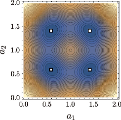
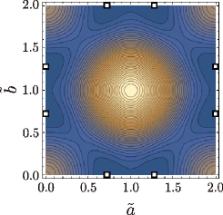
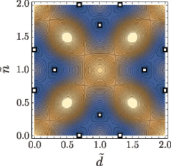
Figure 1: The color contour plots of the one-loop effective potentials as functions of the parametrized zero modes of $A_{5}$ in $SU(7)$ model with ${\mathcal{N}}_{7}=(0,0,0,0,2,0,0,0)$ (left), $SO(10)$ model with ${\mathcal{N}}_{10}=(0,1,0,0,1,0)$ (center), and $E_{6}$ model with ${\mathcal{N}}_{E_{6}}=(0,4,1,2)$ (right). From light orange region to dark blue region, values of the potential decrease. In each figure, we show positions of the global minima of the potential by the square symbols.

In the $SU(8)$ model, the residual symmetry is $SU(5)\times SU(3)\times U(1)$, which is broken to $G_{\rm SM}$ by VEVs $a_{1}=a_{2}=a_{3}\neq 0$ $({\rm mod}~{}1)$. For instance, the symmetry breaking is achieved for the cases with ${\mathcal{N}}_{8}=(0,0,0,0,2,0,0,0)$ and ${\mathcal{N}}_{8}=(2,0,0,2,0,0,2,0)$. Around the vacua, the mass matrix of the physical mass spectrum of the zero mode of $A_{5}$ is evaluated from $V_{8}(a_{i},{\mathcal{N}}_{8})$ similarly to Eq. (5.1). In Table 1, the VEVs and squared mass eigenvalues are shown for the above two cases. In the eigenvalues, there appears degeneracy, which reflects that two linear combinations of the parametrized VEVs $a_{1,2,3}$ belong to the adjoint representation of $SU(3)_{C}$ in $G_{\rm SM}$.

The $SO(10)$ model has the residual symmetry $SU(5)\times U(1)$. For the cases where one of the parameters $\tilde{a}$ and $\tilde{b}$ in Eq. (3.48) has a non-zero VEV (mod 1) while the other remains zero (mod 2), then $G_{\rm SM}$ is obtained. In Table 1, we show the examples of the matter contents and corresponding VEVs that lead to $G_{\rm SM}$. For the case with ${\mathcal{N}}_{10}=(0,1,0,0,1,0)$, we also show the contour plot of the effective potential in Figure 1 center, where the square symbols indicate the positions of degenerate vacua, which are physically equivalent. Around the vacua, one can evaluate the physical mass spectrum of $A_{5}$ using the potential $V_{10}(\tilde{a},\tilde{b},{\mathcal{N}}_{10})$ similarly to Eq. (5.1). The eigenvalues of the squared masses are also shown in Table 1.

Finally we discuss the $E_{6}$ model, where $\tilde{d}$ and $\tilde{n}$ in Eq. (4.14) parametrize the VEVs. The residual symmetry of the model is $SU(5)_{F}\times U(1)_{V_{F}}$. We are particularly interested in the vacua that lead to $G_{\rm SM}$, where VEVs are $\tilde{d}=0$ (mod 2) and $\tilde{n}\neq 0$ (mod 1). We show two cases with ${\mathcal{N}}_{E_{6}}=(0,2,1,2)$ and ${\mathcal{N}}_{E_{6}}=(0,4,1,2)$ in Table 1. For the latter case, the contour plot of $V_{E_{6}}(\tilde{d},\tilde{n},{\mathcal{N}}_{E_{6}})$ is also shown in Figure 1 right. One can confirm that the potential has the invariance that was mentioned in Sec. 4.3. Around the vacua of the potential, physical components of the zero mode of $A_{5}$ become massive. The VEVs and the squared mass eigenvalues are shown in Table 1.

6 Summary and discussion

We have studied the five-dimensional gGHU models, namely the applications of the Hosotani mechanism to the unified gauge symmetry breaking, on the orbifold compactification $S^{1}/\mathbb{Z}_{2}$. In these models, VEVs of the zero modes of the extra-dimensional gauge fields, whose dynamics reflects degrees of freedom of Wilson line phases, are available to break the residual symmetry. The effective potential of the zero mode is generated by quantum corrections that depend on matter contents in the models.

We have discussed the models based on $SU(7)$, $SU(8)$, $SO(10)$, and $E_{6}$ gauge symmetries. In each model, the standard model gauge symmetry is achieved at a low-energy regime when the suitable bulk fermion fields are contained. We have derived the one-loop effective potentials for the zero modes of the extra-dimensional gauge fields in all the models. We have also studied the effects of the localized mass term for the gauge field induced by the anomaly in the $E_{6}$ model.

We have analyzed vacuum structures of the effective potentials and shown examples of the matter contents for bulk fermion fields that lead to the non-trivial VEVs of the zero modes and the standard model gauge symmetry at the vacua. Our discussions have shown that not so many bulk fermions are required to achieve the desired vacua; it implies that the unified symmetry is naturally broken by dynamics of the Wilson line phases, owing to extra dimensions in our Universe.

To make our discussion more concrete, the mass spectrum of the bulk fermion fields and the standard model matter sector should be explicitly treated. In this case, one can examine the renormalization group evolution of the gauge coupling constants, which has large dependence on the bulk fermion mass spectrum. Since the mass spectrum is not severely constrained, we tend to lose precise predictions for the values of the gauge couplings in this setup. For instance, if we introduce bulk masses for bulk fermion fields slightly smaller than the compactification scale, which do not change the present analysis of the effective potentials approximately, their contributions to the evolution are suppressed. The standard model fermions and the Higgs scalar can be introduced into the models as bulk fields or localized fields in the present setup. As mentioned, the models based on $SU(N)$ $(N=7,8)$ and $SO(10)$ share a part of symmetry breaking pattern with the product GUT models [16] and the flipped $SU(5)$ models [17], respectively, although the construction of the hypercharge generator in our models is different from the known models. This implies that the standard model fields are realized as boundary localized fields in our $SU(N)$ and $SO(10)$ models. On the other hand, the standard model fields are naturally incorporated into bulk fields in the $E_{6}$ model. In addition, the supersymmetric extension of the $E_{6}$ model can supply the doublet-triplet splitting via an analogues of the missing partner mechanism that is often discussed in the flipped $SU(5)$ models. These subjects are left to our future studies.

Acknowledgments

The authors would like to thank N. Yamatsu for valuable discussions.

Appendix A Calculation of the effective potential in the $E_{6}$ model

A.1 Contributions from bulk fermion fields

In Sec. 4.3, the contribution to the effective potential from bulk fermion fields in the $E_{6}$ model is shown, with the help of the effective potential in the $SO(10)$ model. In this subsection, we derive the contribution by using another explicit formulation.

For deriving the contribution, a key point is that the $U(1)$ directions accompanied by $\tilde{d}$ and $\tilde{n}$ in Eq. (4.14) are identified to generators in $SU(6)$ and $SU(2)_{E}$, respectively. This can be realized because the zero mode of $A_{5}$ appears in the adjoint representations of $SU(6)$ and $SU(2)_{E}$. To see this, we first focus on the decomposition of $A_{\mu}$ in Eqs. (4.7)–(4.10). It is useful to consider the $U(1)_{Y_{F}}$ subgroup that appears in $SU(5)_{F}\supset SU(3)_{C}\times SU(2)_{L}\times U(1)_{Y_{F}}$. One can further decompose the $SU(5)_{F}\times U(1)_{V_{F}}$ representations of $A_{\mu}$ as

$$A_{\mu}(24_{0})^{(+,+)} =A_{\mu}(G)^{(+,+)}+A_{\mu}(W)^{(+,+)}+A_{\mu}(n_{Y_{F}})^{(+,+)}+A_{\mu}(Q)^{(+,+)}+A_{\mu}(\overline{Q})^{(+,+)},$$ (A.1)

$$A_{\mu}(1^{V_{F}}_{0})^{(+,+)} =A_{\mu}(n_{V_{F}})^{(+,+)},$$ (A.2)

$$A_{\mu}(10_{-4})^{(+,-)} =A_{\mu}(X)^{(+,-)}+A_{\mu}(\overline{U})^{(+,-)}+A_{\mu}(E)^{(+,-)},$$ (A.3)

$$A_{\mu}(\overline{10}_{4})^{(+,-)} =A_{\mu}(\overline{X})^{(+,-)}+A_{\mu}({U})^{(+,-)}+A_{\mu}(\overline{E})^{(+,-)},$$ (A.4)

$$A_{\mu}(1^{V^{\prime}}_{0})^{(+,+)} =A_{\mu}(n_{V^{\prime}})^{(+,+)},$$ (A.5)

$$A_{\mu}(10_{1})^{(-,-)} =A_{\mu}(q)^{(-,-)}+A_{\mu}(\overline{d})^{(-,-)}+A_{\mu}(\overline{n})^{(-,-)},$$ (A.6)

$$A_{\mu}(\overline{5}_{-3})^{(-,+)} =A_{\mu}(\overline{u})^{(-,+)}+A_{\mu}({\ell})^{(-,+)},$$ (A.7)

$$A_{\mu}(1_{5})^{(-,+)} =A_{\mu}(\overline{e})^{(-,+)},$$ (A.8)

$$A_{\mu}(\overline{10}_{-1})^{(-,-)} =A_{\mu}(\overline{q})^{(-,-)}+A_{\mu}({d})^{(-,-)}+A_{\mu}({n})^{(-,-)},$$ (A.9)

$$A_{\mu}(5_{3})^{(-,+)} =A_{\mu}({u})^{(-,+)}+A_{\mu}(\overline{\ell})^{(-,+)},$$ (A.10)

$$A_{\mu}(1_{-5})^{(-,+)} =A_{\mu}({e})^{(-,+)},$$ (A.11)

where $A_{\mu}(R)$ in the right-hand sides transforms as $R$ in Table 2 under the $SU(3)_{C}\times SU(2)_{L}\times U(1)_{Y_{F}}\times U(1)_{V_{F}}$ symmetry. We denote the complex conjugate of $R$ by $\overline{R}$. Note that the $U(1)_{Y}$ hypercharge and the charge of the Cartan generator of $SU(2)_{R}$, which we denote by $T^{3}_{R}$, are linear combinations of $U(1)_{Y_{F}}$ and $U(1)_{V_{F}}$ charges; they are also shown in Table 2. One can see that $SU(3)_{C}\times SU(2)_{L}$ gauge fields correspond to the zero modes of $A_{\mu}(G)^{(+,+)}$ and $A_{\mu}(W)^{(+,+)}$, and the $U(1)_{Y}$ gauge field is a linear combination of the zero modes of $A_{\mu}(n_{Y_{F}})^{(+,+)}$ and $A_{\mu}(n_{V_{F}})^{(+,+)}$. If the symmetry breaking $SU(5)_{F}\times U(1)_{V_{F}}\to G_{\rm SM}$ is realized, then the zero modes $A_{\mu}(Q)^{(+,+)}$, $A_{\mu}(\overline{Q})^{(+,+)}$, and a linear combination of $A_{\mu}(n_{Y_{F}})^{(+,+)}$ and $A_{\mu}(n_{V_{F}})^{(+,+)}$ become massive with would-be NG bosons that belong to the zero mode of $A_{5}$.

Table 2: Representations and charges under $SU(3)_{C}$, $SU(2)_{L}$, $U(1)_{Y_{F}}$, $U(1)_{V_{F}}$, $U(1)_{Y}$, and $T^{3}_{R}$.

	$G$	$W$	$n_{Y_{F}}$	$Q$	$n_{V_{F}}$	$U$	$X$	$E$	$n_{V^{\prime}}$	$d$	$q$	$n$	$u$	$\ell$	$e$
$SU(3)_{C}$	8	1	1	3	1	3	3	1	1	3	3	1	3	1	1
$SU(2)_{L}$	1	3	1	2	1	1	2	1	1	1	2	1	1	1	1
$U(1)_{Y_{F}}$	0	0	0	$-{5\over 6}$	0	${2\over 3}$	${1\over 6}$	$1$	0	${2\over 3}$	${1\over 6}$	$-1$	$-{1\over 3}$	$-{1\over 2}$	$0$
$U(1)_{V_{F}}$	0	0	0	0	0	4	$-4$	$-4$	0	$-1$	$1$	$-1$	$3$	$-3$	$-5$
$U(1)_{Y}$	0	0	0	${1\over 6}$	0	${2\over 3}$	$-{5\over 6}$	$-1$	0	$-{1\over 3}$	${1\over 6}$	$0$	${2\over 3}$	$-{1\over 2}$	${-1}$
$T^{3}_{R}$	0	0	0	$-{1\over 2}$	0	0	${1\over 2}$	$1$	0	${1\over 2}$	$0$	$-{1\over 2}$	$-{1\over 2}$	$0$	${1\over 2}$

We next focus on the $SU(6)_{F}\times SU(2)_{E_{F}}$ decomposition of $A_{5}$. Similarly to $A_{\mu}$ in Eqs. (4.11)–(4.13), we can obtain

$$A_{5}((35,1)) =A_{5}(24_{0})^{(-,-)}+A_{5}(5_{3})^{(+,-)}+A_{5}(\overline{5}_{-3})^{(+,-)}+A_{5}(1^{K_{F}}_{0})^{(-,-)},$$ (A.12)

$$A_{5}((1,3)) =A_{5}(1_{5})^{(+,-)}+A_{5}(1_{-5})^{(+,-)}+A_{5}(1^{E_{F}}_{0})^{(-,-)},$$ (A.13)

$$A_{5}((20,2)) =A_{5}(10_{1})^{(+,+)}+A_{5}(\overline{10}_{-1})^{(+,+)}+A_{5}(10_{-4})^{(-,+)}+A_{5}(\overline{10}_{4})^{(-,+)}.$$ (A.14)

These equations can be rewritten by the representations in Table 2 as

$$A_{5}((35,1))= A_{5}(G)^{(-,-)}+A_{5}(W)^{(-,-)}+A_{5}(n_{Y_{F}})^{(-,-)}+A_{5}(Q)^{(-,-)}+A_{5}(\overline{Q})^{(-,-)}$$

$$+A_{5}({u})^{(+,-)}+A_{5}(\overline{\ell})^{(+,-)}+A_{5}(\overline{u})^{(+,-)}+A_{5}({\ell})^{(+,-)}+A_{5}({n_{K_{F}}})^{(-,-)},$$ (A.15)

$$A_{5}((1,3))= A_{5}(\overline{e})^{(+,-)}+A_{5}({e})^{(+,-)}+A_{5}({n_{E_{F}}})^{(-,-)},$$ (A.16)

$$A_{5}((20,2))= A_{5}(q)^{(+,+)}+A_{5}(\overline{d})^{(+,+)}+A_{5}(\overline{n})^{(+,+)}+A_{5}(\overline{q})^{(+,+)}+A_{5}({d})^{(+,+)}+A_{5}({n})^{(+,+)}$$

$$+A_{5}(X)^{(-,+)}+A_{5}(\overline{U})^{(-,+)}+A_{5}({E})^{(-,+)}+A_{5}(\overline{X})^{(-,+)}+A_{5}({U})^{(-,+)}+A_{5}(\overline{E})^{(-,+)},$$ (A.17)

where $A_{5}({n_{K_{F}}})^{(-,-)}$ and $A_{5}({n_{E_{F}}})^{(-,-)}$ are linear combinations of $A_{5}(n_{V_{F}})^{(-,-)}$ and $A_{5}(n_{V^{\prime}})^{(-,-)}$. From the expression, using the $SU(2)_{R}$ flip, we can obtain the $E_{6}\supset SU(6)\times SU(2)_{E}$ decomposition of $A_{5}$:

$$A_{5} =A_{5}((35,1)^{\prime})+A_{5}((1,3)^{\prime})+A_{5}((20,2)^{\prime}),$$ (A.18)

where the terms in the right-hand side transform as the irreducible representations of $SU(6)\times SU(2)_{E}$. They are rewritten as follows:

$$A_{5}((35,1)^{\prime})= A_{5}(G)^{(-,-)}+A_{5}(W)^{(-,-)}+A_{5}(n_{Y})^{(-,-)}+A_{5}(X)^{(-,+)}+A_{5}(\overline{X})^{(-,+)}$$

$$+A_{5}({d})^{(+,+)}+A_{5}(\overline{\ell})^{(+,-)}+A_{5}(\overline{d})^{(+,+)}+A_{5}({\ell})^{(+,-)}+A_{5}({n_{K}})^{(-,-)},$$ (A.19)

$$A_{5}((1,3)^{\prime})= A_{5}(\overline{n})^{(+,+)}+A_{5}({n})^{(+,+)}+A_{5}({n_{E}})^{(-,-)},$$ (A.20)

$$A_{5}((20,2)^{\prime})= A_{5}(q)^{(+,+)}+A_{5}(\overline{u})^{(+,-)}+A_{5}(\overline{e})^{(+,-)}+A_{5}(\overline{q})^{(+,+)}+A_{5}({u})^{(+,-)}+A_{5}({e})^{(+,-)}$$

$$+A_{5}(Q)^{(-,-)}+A_{5}(\overline{U})^{(-,+)}+A_{5}(\overline{E})^{(-,+)}+A_{5}(\overline{Q})^{(-,-)}+A_{5}({U})^{(-,+)}+A_{5}({E})^{(-,+)}.$$ (A.21)

In this expression, $A_{5}({n_{Y_{F}}})^{(-,-)}$, $A_{5}({n_{K_{F}}})^{(-,-)}$, and $A_{5}({n_{E_{F}}})^{(-,-)}$ are rearranged as $A_{5}({n_{Y}})^{(-,-)}$, $A_{5}({n_{K}})^{(-,-)}$, and $A_{5}({n_{E}})^{(-,-)}$. One can now clearly see that $\tilde{d}$ and $\tilde{n}$ in Eq. (4.14), which parametrize the zero mode of $A_{5}$ and thus are involved in the parity $(+,+)$ fields in Eqs. (A.19)–(A.21), belong to the gauge field of an $SU(2)$ subgroup of $SU(6)$ and $SU(2)_{E}$, respectively; these $SU(2)$ symmetries are just what we called $SU(2)_{d}$ and $SU(2)_{n}$ below Eq. (4.14).

Let us derive the contributions to the effective potential for $\tilde{d}$ and $\tilde{n}$ from a bulk adjoint field $\Phi_{A}^{(\tilde{\eta})}$, where $\tilde{\eta}$ is a parameter related to the periodicity of the field. For this purpose, we show the transformation law of $\Phi_{A}^{(\tilde{\eta})}$ under $SU(2)_{d}\times SU(2)_{n}$ accompanied by the periodicity of the field, explicitly. The adjoint field is decomposed into $SU(6)\times SU(2)_{E}$ representations as

$$\Phi_{A}^{(\tilde{\eta})} =\Phi_{A}^{(\tilde{\eta})}((35,1)^{\prime})+\Phi_{A}^{(\tilde{\eta})}((1,3)^{\prime})+\Phi_{A}^{(\tilde{\eta})}((20,2)^{\prime}).$$ (A.22)

One can further decompose the fields as

$$\Phi_{A}^{(\tilde{\eta})}((35,1)^{\prime})= \Phi_{A}(G)^{(+\tilde{\eta})}+\Phi_{A}(W)^{(+\tilde{\eta})}+\Phi_{A}(n_{Y})^{(+\tilde{\eta})}+\Phi_{A}(X)^{(-\tilde{\eta})}+\Phi_{A}(\overline{X})^{(-\tilde{\eta})}$$

$$+\Phi_{A}({d})^{(+\tilde{\eta})}+\Phi_{A}(\overline{\ell})^{(-\tilde{\eta})}+\Phi_{A}(\overline{d})^{(+\tilde{\eta})}+\Phi_{A}({\ell})^{(-\tilde{\eta})}+\Phi_{A}({n_{K}})^{(+\tilde{\eta})},$$ (A.23)

$$\Phi_{A}^{(\tilde{\eta})}((1,3)^{\prime})= \Phi_{A}(\overline{n})^{(+\tilde{\eta})}+\Phi_{A}({n})^{(+\tilde{\eta})}+\Phi_{A}({n_{E}})^{(+\tilde{\eta})},$$ (A.24)

$$\Phi_{A}^{(\tilde{\eta})}((20,2)^{\prime})= \Phi_{A}(q)^{(+\tilde{\eta})}+\Phi_{A}(\overline{u})^{(-\tilde{\eta})}+\Phi_{A}(\overline{e})^{(-\tilde{\eta})}+\Phi_{A}(\overline{q})^{(+\tilde{\eta})}+\Phi_{A}({u})^{(-\tilde{\eta})}+\Phi_{A}({e})^{(-\tilde{\eta})}$$

$$+\Phi_{A}(Q)^{(+\tilde{\eta})}+\Phi_{A}(\overline{U})^{(-\tilde{\eta})}+\Phi_{A}(\overline{E})^{(-\tilde{\eta})}+\Phi_{A}(\overline{Q})^{(+\tilde{\eta})}+\Phi_{A}({U})^{(-\tilde{\eta})}+\Phi_{A}({E})^{(-\tilde{\eta})},$$ (A.25)

where in the right-hand sides $\pm\tilde{\eta}$ denotes the periodicity that coincides with the eigenvalue of the translation operator $\hat{P}_{1}\hat{P}_{0}$.

From the above expression, we can easily see the $SU(2)_{n}$ transformation law of $\Phi_{A}^{(\tilde{\eta})}$ with the periodicity. In $\Phi_{A}^{(\tilde{\eta})}((1,3)^{\prime})$, there is one triplet of the periodicity $+\tilde{\eta}$. In $\Phi_{A}^{(\tilde{\eta})}((20,2)^{\prime})$, there are twenty doublets, of which the twelve have $+\tilde{\eta}$ and the rest have $-\tilde{\eta}$.

For $SU(2)_{d}$, a little difficulty remains; the transformation law is not manifest in Eqs. (A.23)–(A.25) since $SU(2)_{d}$ does not commute with $SU(3)_{C}$. Fortunately, we can find another $SU(2)$ that helps us to see the $SU(2)_{d}$ transformation law of each $SU(6)\times SU(2)_{E}$ representation in Eqs. (A.23)–(A.25) taking account of the periodicity $\pm\tilde{\eta}$. Note that the $SU(4)$ subgroup in $SU(6)/SU(2)_{L}$ commutes with the translation operator $\hat{P}_{1}\hat{P}_{0}$ and involves both $SU(3)_{C}$ and $SU(2)_{d}$. This implies that using any $SU(2)$ subgroup of $SU(3)_{C}$ instead of $SU(2)_{d}$, we can derive the $SU(2)_{d}$ transformation law of each $SU(6)\times SU(2)_{E}$ representation with the periodicity. Accordingly, under $SU(2)_{d}$, it is realized that there are one triplet of $+\tilde{\eta}$, four doublets of $+\tilde{\eta}$, and four doublets of $-\tilde{\eta}$ in $\Phi_{A}^{(\tilde{\eta})}((35,1)^{\prime})$. For $\Phi_{A}^{(\tilde{\eta})}((20,2)^{\prime})$, eight doublets of $+\tilde{\eta}$ and four doublets of $-\tilde{\eta}$ are contained. Among the doublets, since $\Phi_{A}^{(\tilde{\eta})}((20,2)^{\prime})$ is also $SU(2)_{n}$ doublet, there are bi-doublets under $SU(2)_{d}\times SU(2)_{n}$; four bi-doublets of $+\tilde{\eta}$ and two bi-doublets of $-\tilde{\eta}$ are contained.

In this way, the decompositions in Eqs. (A.23)–(A.25) tell us the transformations of the fields under $SU(2)_{d}\times SU(2)_{n}$. The result is

$$\Phi_{A}^{(\tilde{\eta})}((35,1)^{\prime}) \ni 4\times\Phi_{A}(2,1)^{(+\tilde{\eta})}+4\times\Phi_{A}(2,1)^{(-\tilde{\eta})}+1\times\Phi_{A}(3,1)^{(+\tilde{\eta})},$$ (A.26)

$$\Phi_{A}^{(\tilde{\eta})}((1,3)^{\prime}) \ni 1\times\Phi_{A}(1,3)^{(+\tilde{\eta})},$$ (A.27)

$$\Phi_{A}^{(\tilde{\eta})}((20,2)^{\prime}) \ni 4\times\Phi_{A}(1,2)^{(+\tilde{\eta})}+4\times\Phi_{A}(1,2)^{(-\tilde{\eta})}+4\times\Phi_{A}(2,2)^{(+\tilde{\eta})}+2\times\Phi_{A}(2,2)^{(-\tilde{\eta})},$$ (A.28)

where in the right-hand sides $\Phi_{A}(R,R^{\prime})$ transforms under $SU(2)_{d}$ $(SU(2)_{n})$ as $R$ $(R^{\prime})$ and the superscript for each term denotes the periodicity. Hence one can obtain

$$\Phi_{A}^{(\pm)}\ni~{} 4\left[\Phi_{A}(2,1)^{(\pm)}+\Phi_{A}(2,1)^{(\mp)}+\Phi_{A}(1,2)^{(\pm)}+\Phi_{A}(1,2)^{(\mp)}\right]$$

$$+4\Phi_{A}(2,2)^{(\pm)}+2\Phi_{A}(2,2)^{(\mp)}+\Phi_{A}(3,1)^{(\pm)}+\Phi_{A}(1,3)^{(\pm)}.$$ (A.29)

From the above, the contribution in Eq. (4.21) is obtained.

The contribution from a 27-plet $\Phi_{F}^{(\tilde{\eta})}$ is obtained in a similar fashion. The field is decomposed into $SU(6)_{F}\times SU(2)_{E_{F}}$ multiplets as

$$\Phi_{F}^{(\tilde{\eta})} =\Phi_{F}^{(\tilde{\eta})}((15,1))+\Phi_{F}^{(\tilde{\eta})}((\overline{6},2)).$$ (A.30)

Further decomposition leads to

$$\Phi_{F}^{(\tilde{\eta})}((15,1)) =\Phi_{F}(q)^{(-\tilde{\eta})}+\Phi_{F}(\overline{d})^{(-\tilde{\eta})}+\Phi_{F}(\overline{n})^{(-\tilde{\eta})}+\Phi_{F}(D)^{(+\tilde{\eta})}+\Phi_{F}(L)^{(+\tilde{\eta})},$$ (A.31)

$$\Phi_{F}^{(\tilde{\eta})}((\overline{6},2)) =\Phi_{F}(\overline{u})^{(+\tilde{\eta})}+\Phi_{F}(\ell)^{(+\tilde{\eta})}+\Phi_{F}(s)^{(-\tilde{\eta})}+\Phi_{F}(\overline{D})^{(-\tilde{\eta})}+\Phi_{F}(\overline{L})^{(-\tilde{\eta})}+\Phi_{F}(\overline{e})^{(+\tilde{\eta})}.$$ (A.32)

In the right-hand sides $\Phi_{F}(R)$ transforms under $SU(3)_{C}\times SU(2)_{L}\times U(1)_{Y_{F}}\times U(1)_{V_{F}}$ symmetry as in Table 2 and 3 and the superscript for each term denotes the periodicity.

Table 3: Representations and charges under $SU(3)_{C}$, $SU(2)_{L}$, $U(1)_{Y_{F}}$, $U(1)_{V_{F}}$, $U(1)_{Y}$, and $T^{3}_{R}$.

	$D$	$L$	$s$
$SU(3)_{C}$	3	1	1
$SU(2)_{L}$	1	2	1
$U(1)_{Y_{F}}$	$-{1\over 3}$	${1\over 2}$	0
$U(1)_{V_{F}}$	$-2$	$-2$	0
$U(1)_{Y}$	$-{1\over 3}$	$-{1\over 2}$	0
$T_{3R}$	$0$	${1\over 2}$	0

Using the $SU(2)_{R}$ flip, we can obtain the $E_{6}\supset SU(6)\times SU(2)_{E}$ decomposition as

$$\Phi_{F}^{(\tilde{\eta})}((15,1)^{\prime}) =\Phi_{F}(q)^{(-\tilde{\eta})}+\Phi_{F}(\overline{u})^{(+\tilde{\eta})}+\Phi_{F}(\overline{e})^{(+\tilde{\eta})}+\Phi_{F}(D)^{(+\tilde{\eta})}+\Phi_{F}(\overline{L})^{(-\tilde{\eta})},$$ (A.33)

$$\Phi_{F}^{(\tilde{\eta})}((\overline{6},2)^{\prime}) =\Phi_{F}(\overline{d})^{(-\tilde{\eta})}+\Phi_{F}(\ell)^{(+\tilde{\eta})}+\Phi_{F}(s)^{(-\tilde{\eta})}+\Phi_{F}(\overline{D})^{(-\tilde{\eta})}+\Phi_{F}(L)^{(+\tilde{\eta})}+\Phi_{F}(\overline{n})^{(-\tilde{\eta})}.$$ (A.34)

Therefore, a 27-plet involves the fields that transform under $SU(2)_{d}\times SU(2)_{n}$ as

$$\Phi_{F}^{(\tilde{\eta})}((15,1)^{\prime}) \ni 2\times\Phi_{F}(2,1)^{(+\tilde{\eta})}+2\times\Phi_{F}(2,1)^{(-\tilde{\eta})},$$ (A.35)

$$\Phi_{F}^{(\tilde{\eta})}((\overline{6},2)^{\prime}) \ni 2\times\Phi_{F}(1,2)^{(+\tilde{\eta})}+2\times\Phi_{F}(1,2)^{(-\tilde{\eta})}+1\times\Phi_{F}(2,2)^{(-\tilde{\eta})}.$$ (A.36)

Thus one can realize

$$\Phi_{F}^{(\pm)} \ni 2\left[\Phi_{F}(2,1)^{(\pm)}+\Phi_{F}(2,1)^{(\mp)}+\Phi_{F}(1,2)^{(\pm)}+\Phi_{F}(1,2)^{(\mp)}\right]+\Phi_{F}(2,2)^{(\mp)}.$$

From the above, we can easily lead to Eq. (4.32).

A.2 Contributions from the gauge field

In this subsection, we show the calculation of the contributions to the effective potential discussed in Sec. 4.4. The contribution is generated by the gauge field, whose $U(1)_{V^{\prime}}$ component is assumed to have a large mass term at the $y=0$ boundary due to the anomaly cancellation. The mass term effectively modifies the boundary condition and the KK masses of some components of the gauge field. Without the boundary mass term, the contribution takes the form of Eq. (4.21) with $\delta=0$, since the gauge field belongs to the adjoint representation. The modification of the KK mass alters a part of the contribution in Eq. (4.21).

As explained in Sec. 4.4, the KK mass spectrum that is affected by the localized mass term is obtained as a solution to the EOM of the following set of the fields:

$$\left(A_{\mu}(n^{(3)}),A_{\mu}(n^{(2)}),A_{\mu}(d^{(3)}),A_{\mu}(d^{(2)}),A_{\mu}(X)\right),$$ (A.37)

where $n^{(3,2)}$, $d^{(3,2)}$, and $X$ imply generators of $SU(2)_{n}$, $SU(2)_{d}$, and $U(1)_{X}$, respectively. For convenience we introduce a column vector $\Phi_{\mu}^{\alpha}$ $(\alpha=1\textrm{--}5)$ that consists of the fields:

$$\Phi_{\mu}^{\alpha}\equiv\left({A_{\mu}(d^{2})-iA_{\mu}(d^{3})\over\sqrt{2}},{A_{\mu}(d^{3})-iA_{\mu}(d^{2})\over\sqrt{2}},A_{\mu}(X),{A_{\mu}(n^{3})-iA_{\mu}(n^{2})\over\sqrt{2}},{A_{\mu}(n^{2})-iA_{\mu}(n^{3})\over\sqrt{2}}\right)^{T}.$$ (A.38)

The Lagrangian in Eq. (2.7) is diagonalized by the vector as

$${\cal L}_{\rm gauge} \ni{1\over 2}\eta^{\mu\nu}(\Phi_{\mu}^{\alpha})^{\dagger}\left[\square\delta^{\alpha\beta}-\tilde{\cal D}^{\alpha\beta}\right]\Phi_{\nu}^{\beta},\qquad\delta^{\alpha\beta}={\rm diag}(1,1,1,1,1),$$ (A.39)

$$\tilde{\cal D}^{\alpha\beta} ={\rm diag}\left((\partial_{5}-i{\tilde{d}/R})^{2},(\partial_{5}+i{\tilde{d}/R})^{2},(\partial_{5})^{2},(\partial_{5}+i{\tilde{n}/R})^{2},(\partial_{5}-i{\tilde{n}/R})^{2}\right).$$ (A.40)

We introduce the KK mode expansion:

$$\Phi_{\mu}^{\alpha}(x,y)=\sum_{n=-\infty}^{\infty}\psi_{\mu}^{(n)}(x)\phi^{\alpha(n)}(y),\qquad(\square+m_{\rm KK}^{(n)2})\psi_{\mu}^{(n)}(x)=0.$$ (A.41)

The solution to the bulk EOM is obtained as follows:

$$\phi^{1(n)}(y) =e^{i\tilde{d}y/R}\left[\xi^{1}\cos(m_{\rm KK}^{(n)}y)+\zeta^{1}\sin(m_{\rm KK}^{(n)}y)\right],$$ (A.42)

$$\phi^{2(n)}(y) =e^{-i\tilde{d}y/R}\left[\xi^{2}\cos(m_{\rm KK}^{(n)}y)+\zeta^{2}\sin(m_{\rm KK}^{(n)}y)\right],$$ (A.43)

$$\phi^{3(n)}(y) =\xi^{3}\cos(m_{\rm KK}^{(n)}y)+\zeta^{3}\sin(m_{\rm KK}^{(n)}y),$$ (A.44)

$$\phi^{4(n)}(y) =e^{-i\tilde{n}y/R}\left[\xi^{4}\cos(m_{\rm KK}^{(n)}y)+\zeta^{4}\sin(m_{\rm KK}^{(n)}y)\right],$$ (A.45)

$$\phi^{5(n)}(y) =e^{i\tilde{n}y/R}\left[\xi^{5}\cos(m_{\rm KK}^{(n)}y)+\zeta^{5}\sin(m_{\rm KK}^{(n)}y)\right],$$ (A.46)

where $\xi^{\alpha}$ and $\zeta^{\alpha}$ $(\alpha=1\textrm{--}5)$ are real constants and $m_{\rm KK}^{(n)}$ is the mass of the $n$-th KK mode.

In order to determine the KK mass $m_{\rm KK}^{(n)}$, the boundary condition at $y=0$ and $\pi R$ should be imposed to the solutions in Eqs. (A.42)–(A.46). In the present case, the condition is simplified in a basis where $U(1)_{V^{\prime}}$ is manifest, since there is a boundary mass term for $A_{\mu}(V^{\prime})$. We introduce the new basis,

$$\Phi_{\mu}^{\prime\alpha}=U^{\alpha\beta}\Phi_{\mu}^{\beta},\qquad U^{\alpha\beta}={1\over 4\sqrt{5}}\begin{pmatrix}2\sqrt{10}&2i\sqrt{10}&0&0&0\\ 4i&4&-4\sqrt{3}&0&0\\ i\sqrt{15}&\sqrt{15}&2\sqrt{5}&\sqrt{15}&i\sqrt{15}\\ 3i&3&2\sqrt{3}&-5&-5i\\ 0&0&0&2i\sqrt{10}&2\sqrt{10}\end{pmatrix},$$ (A.47)

and we denote

$$\Phi_{\mu}^{\prime\alpha} =(A_{\mu}(d^{2}),A_{\mu}(K^{\prime}),A_{\mu}(V^{\prime}),A_{\mu}(V),A_{\mu}(n^{2}))^{T},$$ (A.48)

where $A_{\mu}(K^{\prime})$, $A_{\mu}(V^{\prime})$, and $A_{\mu}(V)$ are defined by

$$\begin{pmatrix}A_{\mu}(K^{\prime})\\ A_{\mu}(K)\end{pmatrix} ={1\over\sqrt{5}}\begin{pmatrix}{\sqrt{2}}&{-\sqrt{3}}\\ {\sqrt{3}}&{\sqrt{2}}\end{pmatrix}\begin{pmatrix}A_{\mu}(d^{3})\\ A_{\mu}(X)\end{pmatrix}, \begin{pmatrix}A_{\mu}(V^{\prime})\\ A_{\mu}(V)\end{pmatrix} ={1\over 4}\begin{pmatrix}{\sqrt{10}}&{\sqrt{6}}\\ {\sqrt{6}}&-{\sqrt{10}}\end{pmatrix}\begin{pmatrix}A_{\mu}(K)\\ A_{\mu}(n^{3})\end{pmatrix}.$$ (A.49)

It is realized that $A_{\mu}(V^{\prime})$ and $A_{\mu}(V)$ correspond to the $U(1)_{V^{\prime}}$ and $U(1)_{V}$ gauge field, respectively. By using the above fields, the boundary condition is simplified; at $y=0$, the condition is written as

$$\Phi_{\mu}^{\prime 1}=\Phi_{\mu}^{\prime 5}=0,\qquad\partial_{y}\Phi_{\mu}^{\prime 2}=\partial_{y}\Phi_{\mu}^{\prime 4}=0,\qquad(2\partial_{y}-M)\Phi_{\mu}^{\prime 3}=0,$$ (A.50)

where $M$ represents the boundary mass parameter. On the other hand, at $y=\pi R$, the condition is written as

$$\Phi_{\mu}^{\prime 1}=\Phi_{\mu}^{\prime 5}=0,\qquad\partial_{y}\Phi_{\mu}^{\prime 2}=\partial_{y}\Phi_{\mu}^{\prime 3}=\partial_{y}\Phi_{\mu}^{\prime 4}=0.$$ (A.51)

Imposing the boundary condition to the solutions in Eqs. (A.42)–(A.46), we can determine the KK mass $m_{\rm KK}^{(n)}$. In our model, we are interested in the case where $M$ is much larger than the compactification scale $1/R$. In this case, we obtain

$$\sin^{2}(m_{\rm KK}^{(n)}\pi R) ={S_{1}\pm S_{2}\over 8},$$ (A.52)

where $S_{1}$ and $S_{2}$ are found in Eq. (4.35). The above equation leads to Eqs. (4.33) and (4.34).

If there were no boundary mass term, the gauge field and a bulk adjoint field with $\delta=0$, which gives the contribution $F^{78}(\tilde{d},\tilde{n},0)$ in Eq. (4.21), have the same KK mass spectrum. In this case, the $n$-th KK masses of the fields in Eq. (A.37) are

$$\bigg{(}{n\pm\tilde{d}\over R}\bigg{)}^{2},\quad\bigg{(}{n\pm\tilde{n}\over R}\bigg{)}^{2},$$ (A.53)

and ${n^{2}/R^{2}}$. In the contribution $F^{78}(\tilde{d},\tilde{n},0)$, the KK masses in Eq. (A.53) are related to the terms proportional to $\hat{f}(2\tilde{d})$ and $\hat{f}(2\tilde{n})$. The boundary mass term alter the KK masses in Eq. (A.53) into the form in Eqs. (4.33) and (4.34). Thus the contribution from the gauge field with a large boundary mass is obtained by the replacement $\hat{f}(2\tilde{d})$ and $\hat{f}(2\tilde{n})$ with $\hat{f}(2\rho_{+})$ and $\hat{f}(2\rho_{-})$ in $F^{78}(\tilde{d},\tilde{n},0)$. The result is shown in Eq. (4.36).

While the above discussions focus on the contributions from $A_{\mu}$, we also incorporate the contributions from $A_{5}$. Although the $U(1)_{V^{\prime}}$ component of $A_{5}$ has neither zero mode nor direct coupling to the localized mass, the boundary condition of the field is modified from the Dirichlet to the Neumann type effectively by a large boundary mass ($M\gg 1/R$). This modification is induced by proper treatment of gauge fixing terms. In ref. [24], a similar situation can be seen in terms of the four-dimensional effective description. In Appendix C, five-dimensional treatment in a simple $U(1)$ case is shown as an illustrative example.

Appendix B Equivalence of vacua in the $E_{6}$ model

As mentioned in Sec. 4.3, the effective potential in the $E_{6}$ model has the invariance and the periodicity under the characteristic transformation $(\tilde{n},\tilde{d})\to(\tilde{n}+1,\tilde{d}+1)$. In this section, we show the invariance of the potential is ensured by the $E_{6}$ gauge transformation.

In a five-dimensional orbifold model, the gauge transformation is generally written by

$$A_{M}(x,y) \to A_{M}^{\prime}(x,y)=\Lambda(x,y)A_{M}(x,y)\Lambda^{\dagger}(x,y)+{i\over g}\Lambda(x,y)\partial_{M}\Lambda^{\dagger}(x,y),$$ (B.1)

where

$$\Lambda(x,y) =\exp\left({i\lambda_{a}(x,y)t^{a}}\right),$$ (B.2)

and $\lambda_{a}(x,y)$ is a five-dimensional gauge transformation function. When the gauge field satisfies the boundary condition given in Eqs. (2.1)–(2.4), then the gauge transformation implies

$$A_{\mu}^{\prime}(x,-y) =P_{0}^{\prime}A_{\mu}^{\prime}(x,y)P_{0}^{\prime{\dagger}}+{i\over g}P_{0}^{\prime}\partial_{\mu}P_{0}^{\prime{\dagger}},\quad A_{\mu}^{\prime}(x,\pi R-y)=P_{1}^{\prime}A_{\mu}^{\prime}(x,\pi R+y)P_{1}^{\prime{\dagger}}+{i\over g}P_{1}^{\prime}\partial_{\mu}P_{1}^{\prime{\dagger}},$$ (B.3)

$$A_{5}^{\prime}(x,-y) =-P_{0}^{\prime}A_{5}^{\prime}(x,y)P_{0}^{\prime{\dagger}}-{i\over g}P_{0}^{\prime}\partial_{5}P_{0}^{\prime{\dagger}},\quad A_{5}^{\prime}(x,\pi R-y)=-P_{1}^{\prime}A_{5}^{\prime}(x,\pi R+y)P_{1}^{\prime{\dagger}}-{i\over g}P_{1}^{\prime}\partial_{5}P_{1}^{\prime{\dagger}},$$ (B.4)

where

$$P_{0}^{\prime}=\Lambda(x,-y)P_{0}\Lambda^{\dagger}(x,y),\qquad P_{1}^{\prime}=\Lambda(x,\pi R-y)P_{1}\Lambda^{\dagger}(x,\pi R+y).$$ (B.5)

Although generally the gauge transformation changes the boundary conditions, one can find the particular gauge transformation such that the relations $P_{0}=P_{0}^{\prime}$ and $P_{1}=P_{1}^{\prime}$ hold and the gauge field is shifted as $A^{\prime}_{M}\neq A_{M}$. In this case, the non-linear terms in Eqs. (B.3) and (B.4) vanish and hence the same boundary conditions are imposed on $A_{M}$ and $A^{\prime}_{M}$. For example, suppose that a vacuum configuration $\left\langle{A_{5}}\right\rangle$ is shifted to $\left\langle{A^{\prime}_{5}}\right\rangle$ by the gauge transformation function that preserves the boundary conditions, then the potential should have degenerate vacua around $\left\langle{A_{5}}\right\rangle$ and $\left\langle{A_{5}}\right\rangle^{\prime}$.

We start to discuss our $E_{6}$ model, where the VEV in Eq. (4.14) can be written as

$$\left\langle{A_{5}}\right\rangle ={1\over gR}(\tilde{d}t_{\tilde{d}}+\tilde{n}t_{\tilde{n}}),$$ (B.6)

where $t_{\tilde{d}}$ and $t_{\tilde{n}}$ are generators of $SU(2)_{d}\subset SU(6)$ and $SU(2)_{n}=SU(2)_{E}$, respectively. In a definite basis of the fundamental representation of $SU(6)\times SU(2)_{E}$, the parity matrix of the boundary condition can be written as follows:

$$P_{0} ={\rm diag}(+1,+1,+1,+1,+1,-1)\otimes{\rm diag}(+1,-1),$$ (B.7)

$$P_{1} ={\rm diag}(+1,+1,+1,-1,-1,-1)\otimes{\rm diag}(+1,-1).$$ (B.8)

Here we take that $t_{\tilde{d}}$ generates mixing between 1st and 6th entries in the $SU(6)$ fundamental representation. As discussed in Sec. 2, the generators and the parity matrix satisfy

$$\{P_{0},t_{\tilde{d}}\}=\{P_{0},t_{\tilde{n}}\}=\{P_{1},t_{\tilde{d}}\}=\{P_{1},t_{\tilde{n}}\}=0,\qquad[t_{\tilde{d}},t_{\tilde{n}}]=0.$$ (B.9)

Let us now consider the gauge transformation

$$\Lambda(x,y) =\exp\left({i{y\over R}(t_{\tilde{d}}+t_{\tilde{n}})}\right).$$ (B.10)

From Eq. (B.1), one can see that the transformation shifts the parameters in Eq. (B.6) as

$$(\tilde{d},\tilde{n})\to(\tilde{d}^{\prime},\tilde{n}^{\prime})=(\tilde{d}+1,\tilde{n}+1).$$ (B.11)

The gauge-transformed field satisfies the boundary condition in Eq. (B.4) with the new parity matrices

$$P_{0}^{\prime} =P_{0},\qquad P_{1}^{\prime}=\exp\left({2\pi it_{\tilde{d}}}\right)\exp\left({2\pi it_{\tilde{n}}}\right)P_{1}.$$ (B.12)

As mentioned above, if $P_{1}^{\prime}=P_{1}$ is satisfied, then the effective potential should have invariance under the shift in Eq. (B.11). This can be shown as follows. In the $SU(6)\times SU(2)_{E}$ representation space in Eqs. (B.7) and (B.8), the matrices $\exp({2\pi it_{\tilde{d}}})$ and $\exp({2\pi it_{\tilde{n}}})$ correspond to $2\pi$ rotations of fundamental representation of $SU(2)_{d}$ and $SU(2)_{E}$, respectively. Thus we obtain

$$\exp\left({2\pi it_{\tilde{d}}}\right) ={\rm diag}(-1,+1,+1,+1,+1,-1)\otimes{\rm diag}(+1,+1),$$ (B.13)

$$\exp\left({2\pi it_{\tilde{n}}}\right) ={\rm diag}(+1,+1,+1,+1,+1,+1)\otimes{\rm diag}(-1,-1).$$ (B.14)

The parity matrix $P_{1}^{\prime}$ explicitly written as follows:

$$P_{1}^{\prime} ={\rm diag}(-1,+1,+1,-1,-1,+1)\otimes{\rm diag}(-1,+1)$$

$$={\rm diag}(+1,-1,-1,+1,+1,-1)\otimes{\rm diag}(+1,-1)$$ (B.15)

$$\to{\rm diag}(+1,+1,+1,-1,-1,-1)\otimes{\rm diag}(+1,-1)=P_{1}.$$ (B.16)

In the last line, we use an $SU(4)\subset SU(6)/SU(2)_{d}$ rotation; this rotation does not change $P_{0}$ and the VEV since both $P_{0}$ and $t_{\tilde{d}}$ commute with the $SU(4)$ subgroup. Although the boundary condition in the $E_{6}$ model is unchanged under the gauge transformation in Eq. (B.10), the transformation shifts the parameters as in Eq. (B.11). Therefore, the effective potential should be invariant against the shift in Eq. (B.11). This leads to the periodicity in the potential.

Appendix C Effective modification of the boundary condition of $A_{5}$ with boundary breaking

In Sec. A.2, we show that the boundary condition of $A_{\mu}$ is effectively modified due to the existence of the boundary mass term. As mentioned, while the $U(1)_{V^{\prime}}$ component of $A_{5}$ does not have zero modes, one can see that the boundary condition of $A_{5}$ is also modified by introducing proper gauge fixing terms in the theory. As a result, one can choose the specific gauge, namely $\xi=1$ shown just below, where the KK masses of $A_{5}$ coincide with those of $A_{\mu}$. Here, we consider a five-dimensional $U(1)$ model compactified on an $S^{1}/{\mathbb{Z}}_{2}$ orbifold, and illustrate the essential feature of the modification in the simple setup.

In the $U(1)$ model, the orbifold parity around the fixed point $y=0$ is expressed as

$$A_{\mu}(-y)=A_{\mu}(y),\qquad A_{5}(-y)=-A_{5}(y).$$ (C.1)

Then, as the $E_{6}$ model discussed in Sec. 4, we study the effect of a mass term localized on this fixed point. Below, we consider an anomaly as the origin of the mass term, while it can be the Higgs mechanism.

The anomaly is assumed to be made harmless via the Green-Schwarz mechanism [20]. Namely, a pseudo-scalar field $\chi$ that transforms non-linearly under the $U(1)$ symmetry and has the Wess-Zumino couplings is introduced on this boundary to cancel the anomaly. Such a scalar field allows the Stückelberg mass term [21] (on the boundary)

$${\cal L}_{\rm St}={1\over 2}M\left(A_{\mu}+{1\over\sqrt{M}}\partial_{\mu}\chi\right)^{2}\delta(y),$$ (C.2)

which is $U(1)$ invariant and thus the naive scale of the mass $M$ is around the cutoff scale of the five-dimensional theory, much larger than the compactification scale. As well-known, such a huge mass repels the wave functions of the lower-laying KK modes of $A_{\mu}$ to modify its boundary condition from the Neumann to the Dirichlet type effectively [22]. Below, we examine the effect on those of $A_{5}$, which does not directly couple to the localized mass due to the orbifold parity. (See Ref. [24] for the same analysis in terms of the KK decomposed language.)

For this purpose, as $A_{5}$ is unphysical except for the zero mode, we should treat the gauge fixing term properly. The mixing terms of the four-dimensional gauge field are

$${\cal L}_{\rm mix}=-\partial_{5}A^{\mu}\partial_{\mu}A_{5}+\sqrt{M}A^{\mu}\partial_{\mu}\chi\delta(y),$$ (C.3)

and we adopt the usual gauge fixing term with a constant gauge parameter $\xi$,

$${\cal L}_{\rm GF}=-{1\over{2\xi}}\left[\partial_{\mu}A^{\mu}-\xi\left(\partial_{5}A_{5}+\sqrt{M}\chi\delta(y)\right)\right]^{2},$$ (C.4)

to remove the above mixing terms (up to surface terms). Then the quadratic terms of $A_{5}$ and $\chi$ become

$${\cal L}_{\rm quad}={1\over 2}A_{5}\left(-\square+\xi\partial_{5}^{2}\right)A_{5}-\delta(y)\left(\xi\sqrt{M}\chi\partial_{5}A_{5}+{1\over 2}\chi\left(\square+\xi M\delta(y)\right)\chi\right).$$ (C.5)

Note that this quadratic part is essentially the same as the one in the case that the mass term originates from the Higgs mechanism, and thus the derivation below is applied also for the case.

Since there is an awkward term proportional to $\delta(y)^{2}$ in the quadratic part, we should regularize the delta function. To be more concrete, we replace the delta function by a finite, sufficiently smooth function $\delta_{\epsilon}(y)$ that vanishes for $\left|y\right|\geq\epsilon$ and is normalized as $\int_{-\epsilon}^{\epsilon}\delta_{\epsilon}(y)dy\sim 1$. The EOMs of $A_{5}$ and $\chi$ are respectively

$$\left(-\square+\xi\partial_{5}^{2}\right)A_{5}(y)+\xi\left(\partial_{5}\delta_{\epsilon}(y)\right)\sqrt{M}\chi=0,$$ (C.6)

$$-\delta_{\epsilon}(y)\left(\xi\sqrt{M}\partial_{5}A_{5}(y)+\left(\square+\xi M\delta_{\epsilon}(y)\right)\chi\right)=0,$$ (C.7)

where the $y$-dependences are explicitly shown. Due to the overall delta function in Eq. (C.7), we may not suppose that the combination in the parenthesis there vanishes for $\left|y\right|\geq\epsilon$, while it does vanish, for instance, at $y=0$ as

$$\xi\sqrt{M}\partial_{5}A_{5}(0)+\left(\square+\xi M\delta_{\epsilon}(0)\right)\chi=0.$$ (C.8)

As often done, we integrate Eq. (C.6), which is an odd function of $y$, over a tiny region $0\leq y\leq z=\cal O(\epsilon)$. Then, the contribution of the regular function, $-\square A_{5}$ is negligible and we get

$$\xi\left[\partial_{5}A_{5}(y)+\delta_{\epsilon}(y)\sqrt{M}\chi\right]^{z}_{0}=0.$$ (C.9)

Using Eq. (C.8) to remove the factor $\delta_{\epsilon}(0)$, we obtain

$$\xi\left(\partial_{5}A_{5}(z)+\delta_{\epsilon}(z)\sqrt{M}\chi\right)+\frac{1}{\sqrt{M}}\square\chi=0.$$ (C.10)

Its integration over again a tiny region, $-\epsilon\leq z\leq\epsilon$, leads to

$$\xi\left(2A_{5}(\epsilon)+\sqrt{M}\chi\right)=0,$$ (C.11)

where we use $A_{5}(-\epsilon)=-A_{5}(\epsilon)$. Operating the four-dimensional Laplacian $\square$ on Eq. (C.11) and applying Eq. (C.10) evaluated at $y=\epsilon$ where the delta function vanishes, we can derive an effective mixed boundary condition

$$2\xi\square A_{5}(\epsilon)-\xi^{2}M\partial_{5}A_{5}(\epsilon)=0.$$ (C.12)

The result shows that $A_{5}$ obeys the Dirichlet boundary condition in the limit $M\to 0$; the condition changes to the Neumann boundary condition in the opposite limit $M\to\infty$. The modification of the boundary condition of $A_{5}$ is in accordance with that of $A_{\mu}$.

References

- [1] H. Georgi and S. L. Glashow, Phys. Rev. Lett. 32 (1974) 438.
- [2] J. C. Pati and A. Salam, Phys. Rev. D 10 (1974) 275 [Erratum-ibid. 11 (1975) 703]
- [3] H. Fritzsch and P. Minkowski, Annals Phys. 93 (1975) 193.
- [4] F. Gursey, P. Ramond and P. Sikivie, Phys. Lett. B 60 (1976) 177; Y. Achiman and B. Stech, Phys. Lett. B 77 (1978) 389; R. Barbieri and D. V. Nanopoulos, Phys. Lett. B 91 (1980) 369.
- [5] N. S. Manton, Nucl. Phys. B 158 (1979) 141.
- [6] D. B. Fairlie, Phys. Lett. B 82 (1979) 97.
- [7] Y. Hosotani, Phys. Lett. B 126 (1983) 309; 129 (1983) 193; Phys. Rev. D 29 (1984) 731; Annals Phys. 190 (1989) 233.
- [8] N. V. Krasnikov, Phys. Lett. B 273 (1991) 246; H. Hatanaka, T. Inami and C. S. Lim, Mod. Phys. Lett. A 13 (1998) 2601; N. Arkani-Hamed, A. G. Cohen and H. Georgi, Phys. Lett. B 513 (2001) 232; I. Antoniadis, K. Benakli and M. Quiros, New J. Phys. 3 (2001) 20; G. R. Dvali, S. Randjbar-Daemi and R. Tabbash, Phys. Rev. D 65 (2002) 064021; G. von Gersdorff, N. Irges and M. Quiros, hep-ph/0206029; Y. Hosotani, hep-ph/0504272; N. Maru and T. Yamashita, Nucl. Phys. B 754 (2006) 127; N. Irges and F. Knechtli, hep-lat/0604006; Y. Hosotani, hep-ph/0607064; Y. Hosotani, N. Maru, K. Takenaga and T. Yamashita, Prog. Theor. Phys. 118 (2007) 1053; Nucl. Phys. B 775 (2007) 283; Y. Hosotani, N. Maru, K. Takenaga and T. Yamashita, Prog. Theor. Phys. 118 (2007) 1053.
- [9] M. Kubo, C. S. Lim and H. Yamashita, Mod. Phys. Lett. A 17 (2002) 2249; C. Csaki, C. Grojean and H. Murayama, Phys. Rev. D 67 (2003) 085012; N. Haba, M. Harada, Y. Hosotani and Y. Kawamura, Nucl. Phys. B 657 (2003) 169 [Erratum-ibid 669 (2003) 381]; N. Haba and Y. Shimizu, Phys. Rev. D 67 (2003) 095001 [Erratum-ibid 69 (2004) 059902]; I. Gogoladze, Y. Mimura and S. Nandi, Phys. Lett. B 560 (2003) 204; C. A. Scrucca, M. Serone and L. Silvestrini, Nucl. Phys. B 669 (2003) 128; R. Contino, Y. Nomura and A. Pomarol, Nucl. Phys. B 671 (2003) 148; N. Haba, Y. Hosotani and Y. Kawamura, Prog. Theor. Phys. 111 (2004) 265; N. Haba and T. Yamashita, JHEP 0404 (2004) 016; Y. Hosotani, S. Noda and K. Takenaga, Phys. Rev. D 69 (2004) 125014; N. Haba, K. Takenaga and T. Yamashita, Phys. Lett. B 605 (2005) 355; Y. Hosotani, S. Noda and K. Takenaga, Phys. Lett. B 607 (2005) 276; N. Haba, K. Takenaga and T. Yamashita, Phys. Lett. B 615 (2005) 247; K. Agashe, R. Contino and A. Pomarol, Nucl. Phys. B 719, 165 (2005); K. Agashe and R. Contino, Nucl. Phys. B 742 (2006) 59; N. Maru and K. Takenaga, Phys. Lett. B 637 (2006) 287; A. D. Medina, N. R. Shah and C. E. M. Wagner, Phys. Rev. D 76 (2007) 095010; Y. Hosotani and Y. Sakamura, Prog. Theor. Phys. 118 (2007) 935; Y. Hosotani, P. Ko and M. Tanaka, Phys. Lett. B 680 (2009) 179; N. Haba, Y. Sakamura and T. Yamashita, JHEP 0907 (2009) 020; JHEP 1003 (2010) 069; N. Haba, S. Matsumoto, N. Okada and T. Yamashita, JHEP 1003 (2010) 064.
- [10] L. J. Hall, Y. Nomura and D. Tucker-Smith, Nucl. Phys. B 639 (2002) 307; G. Burdman and Y. Nomura, Nucl. Phys. B 656 (2003) 3; N. Haba, Y. Hosotani, Y. Kawamura and T. Yamashita, Phys. Rev. D 70 (2004) 015010; C. S. Lim and N. Maru, Phys. Lett. B 653 (2007) 320; Y. Hosotani and N. Yamatsu, PTEP 2015 (2015) 111B01; N. Yamatsu, PTEP 2016 (2016) no.4, 043B02.
- [11] K. Kojima, K. Takenaga and T. Yamashita, Phys. Rev. D 84 (2011) 051701; Phys. Rev. D 95 (2017) no.1, 015021.
- [12] T. Yamashita, Phys. Rev. D 84 (2011) 115016; M. Kakizaki, S. Kanemura, H. Taniguchi and T. Yamashita, Phys. Rev. D 89 (2014) no.7, 075013.
- [13] Y. Kawamura, Prog. Theor. Phys. 103 (2000) 613; 105 (2001) 691; 105 (2001) 999; L. J. Hall and Y. Nomura, Phys. Rev. D 64 (2001) 055003; 65 (2002) 125012.
- [14] K. R. Dienes and J. March-Russell, Nucl. Phys. B 479 (1996) 113; D. C. Lewellen, Nucl. Phys. B 337 (1990) 61; G. Aldazabal, A. Font, L. E. Ibanez and A. M. Uranga, Nucl. Phys. B 452 (1995) 3; J. Erler, Nucl. Phys. B 475 (1996) 597; Z. Kakushadze and S. H. H. Tye, Phys. Rev. D 55 (1997) 7878; Phys. Rev. D 55 (1997) 7896; M. Ito, S. Kuwakino, N. Maekawa, S. Moriyama, K. Takahashi, K. Takei, S. Teraguchi and T. Yamashita, Phys. Rev. D 83 (2011) 091703; JHEP 1112 (2011) 100.
- [15] N. Haba and T. Yamashita, JHEP 0402 (2004) 059.
- [16] T. Yanagida, Phys. Lett. B 344 (1995) 211; J. Hisano and T. Yanagida, Mod. Phys. Lett. A 10 (1995) 3097; K. I. Izawa and T. Yanagida, Prog. Theor. Phys. 97 (1997) 913.
- [17] S. M. Barr, Phys. Lett. B 112 (1982) 219; J. P. Derendinger, J. E. Kim and D. V. Nanopoulos, Phys. Lett. B 139 (1984) 170; I. Antoniadis, J. R. Ellis, J. S. Hagelin and D. V. Nanopoulos, Phys. Lett. B 194 (1987) 231.
- [18] R. Slansky, Phys. Rept. 79 (1981) 1; N. Yamatsu, arXiv:1511.08771 [hep-ph].
- [19] N. Arkani-Hamed, A. G. Cohen and H. Georgi, Phys. Lett. B 516 (2001) 395; C. A. Scrucca, M. Serone, L. Silvestrini and F. Zwirner, Phys. Lett. B 525 (2002) 169.
- [20] M. B. Green and J. H. Schwarz, Phys. Lett. B 149 (1984) 117.
- [21] E. C. G. Stueckelberg, Helv. Phys. Acta 11 (1938) 225.
- [22] Y. Nomura, D. Tucker-Smith and N. Weiner, Nucl. Phys. B 613 (2001) 147; C. Csaki, C. Grojean, H. Murayama, L. Pilo and J. Terning, Phys. Rev. D 69 (2004) 055006.
- [23] Y. Kawamura and T. Miura, Int. J. Mod. Phys. A 28 (2013) 1350055.
- [24] A. Muck, A. Pilaftsis and R. Ruckl, Phys. Rev. D 65 (2002) 085037.
- [25] G. Cacciapaglia, C. Csaki, C. Grojean, M. Reece and J. Terning, Phys. Rev. D 72 (2005) 095018.
- [26] N. Haba, Y. Sakamura and T. Yamashita, JHEP 0806 (2008) 044.