A NASA Perspective on Quantum Computing: Opportunities and Challenges

Abstract

In the last couple of decades, the world has seen several stunning instances of quantum algorithms that provably outperform the best classical algorithms. For most problems, however, it is currently unknown whether quantum algorithms can provide an advantage, and if so by how much, or how to design quantum algorithms that realize such advantages. Many of the most challenging computational problems arising in the practical world are tackled today by heuristic algorithms that have not been mathematically proven to outperform other approaches but have been shown to be effective empirically. While quantum heuristic algorithms have been proposed, empirical testing becomes possible only as quantum computation hardware is built. The next few years will be exciting as empirical testing of quantum heuristic algorithms becomes more and more feasible. While large-scale universal quantum computers are likely decades away, special-purpose quantum computational hardware has begun to emerge that will become more powerful over time, as well as some small-scale universal quantum computers.

1 Introduction

In the last couple of decades, the world has seen several stunning instances of quantum algorithms that provably outperform the best classical algorithms. For most problems, however, it is currently unknown whether quantum algorithms can provide an advantage, and if so by how much, or how to design quantum algorithms that realize such advantages. Many of the most challenging computational problems arising in the practical world are tackled today by heuristic algorithms that have not been mathematically proven to outperform other approaches but have been shown to be effective empirically. While quantum heuristic algorithms have been proposed, empirical testing becomes possible only as quantum computation hardware is built. The next few years will be exciting as empirical testing of quantum heuristic algorithms becomes more and more feasible. While large-scale universal quantum computers are likely decades away, special-purpose quantum computational hardware has begun to emerge that will become more powerful over time, as well as some small-scale universal quantum computers.

Successful NASA missions require solution of many challenging computational problems. The ambitiousness of such future missions depends on our ability to solve yet more challenging computational problems to support better and greater autonomy, space vehicle design, rover coordination, air traffic management, anomaly detection, large data analysis and data fusion, and advanced mission planning and logistics. To support NASA’s substantial computational needs, NASA Ames Research Center has a world-class supercomputing facility with one of the world’s most powerful supercomputers. In 2012, NASA established its Quantum Artificial Intelligence Laboratory (QuAIL) at Ames to explore the potential of quantum computing for computational challenges arising in future agency missions. The following year, through a collaboration with Google and USRA, NASA hosted one of the earliest quantum annealer prototypes, a 509-qubit D-Wave II machine, which last summer was upgraded to a 1097-qubit D-Wave 2X system.

Because quantum annealers are the most advanced quantum computational hardware to date, the main focus for the QuAIL team has been on both theoretical and empirical investigations of quantum annealing, from deeper understanding of the computational role of certain quantum effects to empirical analyses of quantum annealer performance on small problems from the domains of planning and scheduling, fault diagnosis, and machine learning. This paper will concentrate on the team’s quantum annealing work, with only brief mention of research related to capabilities of other near-term quantum computational hardware that will be able to run quantum heuristic algorithms beyond quantum annealing. For information on quantum computing more generally, and other algorithms, both heuristic and non, see quantum computing texts such as [1].

The power of quantum computation comes from encoding information in a non-classical way, in qubits, that enable computations to take advantage of purely quantum effects, such as quantum tunneling, quantum interference, and quantum entanglement, that are not available classically. The beauty of quantum annealers is that users can program them without needing to know about the underlying quantum mechanical effects. Knowledge of quantum mechanics aids in more effective programming, just as an understanding of compilation procedures can aid classical programming, but it is not necessary for a basic understanding.

For this reason, the first three sections consist of an overview of quantum annealing (Sec. 2), a description of how to program a quantum annealer (Sec. 3), and a high-level review of our exploration of three potential application areas for quantum annealing (Sec. 4). The quantum effects involved are only lightly mentioned, so these sections should be easily accessible to computer scientists without any knowledge of quantum mechanics or quantum computing. Sec. 5, which examines the role various physical processes play in quantum annealing, requires more physics knowledge for a full understanding, as does Sec. 6 that discusses hardware, though a classically-trained computer scientist without knowledge of quantum mechanics can get a high-level understanding. We conclude with a brief section summarizing the outlook for the future.

2 Quantum annealing

Quantum annealing [2, 3] is a metaheuristic optimization algorithm that makes use of quantum effects such as quantum tunneling and interference. It is one of the most accessible quantum algorithms to people versed in classical computing because of its close ties to classical optimization algorithms such as simulated annealing and because the most basic aspects of the algorithm can be captured by a classical cost function and parameter setting. Quantum annealers are special-purpose quantum computational devices that can run only the quantum annealing metaheuristic. For readers not familiar with quantum annealing in physics, we refer to Sec. 5.1 for a general introduction.

Quantum annealers are designed to minimize Quadratic Unconstrained Binary Optimization (QUBO) problems; i.e., the cost function is of the form

$$C(\mathbf{x})=\sum_{i}a_{i}x_{i}+\sum_{i<j}b_{i,j}x_{i}x_{j},$$ (1)

where $\left\{a_{i},b_{i,j}\right\}$ are real coefficients and $\mathbf{x}\in\{0,1\}^{n}$ is a vector of binary-valued variables. An application problem must be mapped to a QUBO before it can be solved on a quantum annealer. For application problems with constraints, the cost function is supplemented with penalty terms that penalize bit strings that do not correspond to valid solutions.

The simplicity of the QUBO formalism belies its expressivity. There exist many techniques for mapping more complicated problems to QUBO:

• A wide class of optimization problems of practical interest can be expressed in terms of cost functions that are polynomials over finite sets of binary variables. Any such function can be re-expressed, through degree-reduction techniques using ancilla variables, as quadratic functions over binary variables. We describe such degree-reduction technique in our section on the CNF mapping of planning problems to QUBO.

• Cost functions involving non-binary, but finite-valued, variables can be rewritten in terms of binary variables alone, and optimization problems with constraints can often be written entirely in terms of cost functions over binary variables through the introduction of slack variables.

For these reasons, the QUBO setting is more general than it may seem. We give examples of QUBO mappings for different applications domains in later sections.

Current quantum annealers such as the D-Wave 2X are fabricated using superconducting materials and operated at tens of milli-Kelvin temperatures. The processors make use of superconducting flux qubits [4] that are superconductor loops sandwiched with Josephson junctions, engineered so that when an external flux is applied, a persistent current appears in the loop. The computational basis of the qubit is the clockwise and counter-clockwise flow of the currents, corresponding to values of +1 and -1, respectively, of the spin variable $s_{j}$ for qubit $j$.

An Ising Hamiltonian

$$H_{1}=\sum_{j}h_{j}s_{j}+\sum_{i,j}J_{i,j}s_{i}s_{j}$$ (2)

can be programmed on the D-Wave system by setting the values of the flux biases $h_{j}$ on each qubit $s_{j}$ and couplings $J_{i,j}$ between qubits. A mapping $s_{j}=2x_{j}-1$ relates an Ising Hamiltonian to a QUBO form. Because only select couplers are implemented in the hardware, only certain quadratic terms can be directly implemented. Embedding, using multiple qubits to represent a single binary variable, is necessary to implement arbitrary QUBOs, a topic we will return to when we discuss programming quantum annealers in more depth.

Quantum annealing is carried out by evolving the system under the time-dependent Hamiltonian

$$H(t)=A(s)H_{0}+B(s)H_{1}$$ (3)

where $H_{1}$ is the problem Hamiltonian in QUBO form and $H_{0}$ is the initial Hamiltonian, which in current annealers is fixed and cannot be set by the programmer. Generally, the Hamiltonian $H_{0}$ is chosen to have a simple energy landscape so that an unsophisticated relaxation process will efficiently put the system in low energy states. During the anneal, $H_{0}$ is gradually changed until it becomes $H_{1}$. The intuition is that if the system starts in low energy states and the change is smooth enough, the system will end up in low energy states of the final Hamiltonian, just as a top spinning on a tray will continue to spin when the tray is moved as long as the change in position is smooth enough. The functions $A(s)$ and $B(s)$ are generally chosen in a way that $H_{0}$ dominates at $s=0$ and $H_{1}$ dominates at $s=1$ (see Fig. 1). Current annealers provide a range of total anneal times $t_{f}$, where $s=t/t_{f}$, enabling traversals at different speeds. On the D-Wave 2X housed at NASA, the annealing time can be chosen in a range from $5~{}\mu$s to $2$ ms. Future annealers may allow programmers to choose $A(s)$ and $B(s)$, but they are currently fixed in the D-Wave 2X.

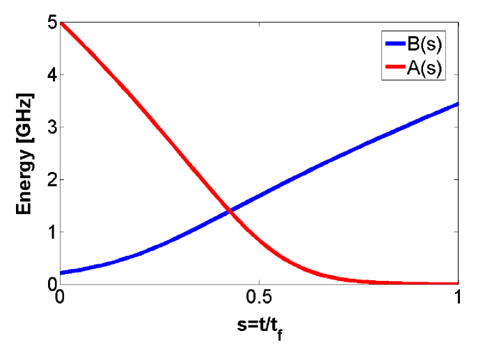
Figure 1: Typical annealing profile $A(s)$ and $B(s)$.

When viewed as an algorithm for exploring the landscape defined by the cost function to find a global minimum, quantum annealing resembles a commonly used classical algorithm for optimization: simulated annealing. While in simulated annealing thermal fluctuation provides the mobility over energy barriers between local minima, quantum annealing has an additional source of mobility: quantum fluctuations that facilitate tunneling through the barriers. Such quantum fluctuations are realized through $H_{0}$ which serves as a driver Hamiltonian responsible for quantum fluctuations because it does not commute with the target Hamiltonian $H_{1}$. As the anneal continues, the driver term is reduced, slowly turning off the fluctuations, as the problem Hamiltonian’s strength increases.

Quantum annealing should not be confused with adiabatic quantum computation which is known to support universal quantum computing. The problem Hamiltonian in quantum annealing typically is a classical Hamiltonian. While adiabatic quantum computation also interpolates between an initial and final Hamiltonian, the final Hamiltonian can be highly non-classical with no analogous classical cost function, thus enabling much more general sorts of quantum computations.

3 Programming a quantum annealer

This section discusses the two main steps in programming a quantum annealer: mapping the problems to QUBO; and embedding, which takes these hardware-independent QUBOs to other QUBOs that match the specific quantum annealing hardware that will be used.

3.1 Mapping

For a cost function not natively in QUBO form, the typical procedure to map the problem into QUBO is to properly choose binary variables, formulate constraints, and embed the violation of constraints as energy penalties. We illustrate this process with an example from Ref. [5].

Example: In a graph coloring problem, the task is to determine whether each vertex of a graph $G(V,E)$ can be colored from a set $\cal C$ so that no two vertices connected by an edge have the same color. The goal is to formulate a cost function such that the minimum is 0. One way to choose the binary variable is to use $x_{v,c}=0$ or $1$ to express whether vertex $v$ is assigned color $c$. The ensuing constraints would be: (1) Each vertex needs to be assigned exactly one color that can be expressed in binary form as $(\sum_{c}x_{v,c}-1)^{2}$. (2) Connected vertices cannot share the same color; otherwise, the energy penalty is raised, $\sum_{c}\sum_{v,v^{\prime}\in E}x_{v,c}x_{v^{\prime},c}$. The cost function expressed in QUBO is then $H=\sum_{v}(\sum_{c}x_{v,c}-1)^{2}+\sum_{c}\sum_{v,v^{\prime}\in E}x_{v,c}x_{v^{\prime},c}$. When no requirement is violated, the cost function has value 0, which is the ground state of $H$.

In this example, the cost function $H$ is naturally quadratic. More generally, the cost functions of many optimization problems can be expressed as higher-degree polynomials of the binary variables (PUBOs). Degree-reduction techniques can then be applied to recast a PUBO as QUBO, usually at the price of adding ancilla variables [6].

3.2 Embedding

Because the physical hardware has limited connectivity, there usually does not exist a direct one-to-one mapping between the QUBO binary variables and the physical qubits so that each binary term in the QUBO corresponds to a pair of connected qubits. To obtain the needed connectivity in the embeddable QUBO, an additional step is required. Unlike the mapping step, the embedding step is hardware dependent. A cluster of qubits $\{y_{i,k}\}$ connected to each other in the hardware graph will represent a single variable $x_{i}$. For any term $x_{i}x_{j}$ in the mapped QUBO, there is a connection in the embeddable QUBO between one of the qubits in the cluster for $x_{i}$ and one qubit in the cluster for $x_{j}$. Minor embedding is the process of determining a cluster for each binary variable in the problem QUBO [7]. The problem of finding the optimal minor embedding is itself NP-complete, but fortunately it is not necessary to find the optimal embedding. In general, for planar architectures, there are straightforward, fast algorithms to embed an $N$-variable problem in hardware consisting of no more than $N^{2}$ physical qubits [7, 8, 9]. In the near term, while the hardware is so qubit constrained, heuristic algorithms [10] are used to try to minimize resources and maximize the size of the problems embeddable on the machine.

To encourage the qubits in the cluster to all take the same value by the end of the anneal so that the value of the variable they represent is unambiguous, the embeddable QUBO also includes constraint terms $J_{F}y_{i,p}y_{i,q}$ for any pair $p,q$ of qubits in the cluster that are connected to each other, where $J_{F}$ is the strength of the coupling. This is to ensure that in the most energy-favorable configuration, all qubits in the cluster take the same value. The Hamiltonian obtained from the embeddable QUBO shares the same ground state energy as the Hamiltonian from the mapped QUBO, but conforms to the hardware architecture. The higher energy spectrum may be considerably altered, so different embeddings can significantly affect performance.

The optimal strength of $J_{F}$ is a subject of extensive research [5, 11, 12]. One might think it should be as high as possible to force the qubits to all take the same value at the end, but in practice there is a sweet spot. Coupling strengths that are too high degrade performance. Intuitively, a high coupling strength makes it harder to change the value of a variable in the cluster once they take on a value that is not, ultimately, optimal, though the actual quantum dynamics are more complicated than this simple explanation.

The layout of the qubits and couplers of a D-Wave quantum annealer is a $n\times n$ lattice of unit cells called a Chimera graph. Each unit cell is composed of a bi-partite graph of 8 qubits. A schematic diagram of the graph formed by 9 cells is shown in Fig. 2. The current D-Wave machine at NASA has $12\times 12$ such units and a total of 1152 qubits, of which 1097 are working. Each qubit is coupled to at most 6 other qubits, 4 within its own unit cell and 2 to qubits in its neighboring cells. To embed a generic QUBO of $N$ variables, $N^{2}$ qubits and couplers are needed in the worst case so that each binary variable can be represented by $N$ physical qubits and effectively couple to all other binary variables. As an illustration, Fig. 3 shows an example of embedding a triangle onto a bi-partite graph.

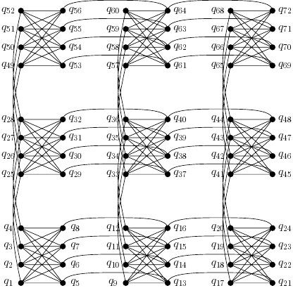
Figure 2: Nine unit cells in a Chimera graph.

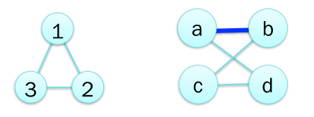
Figure 3: Schematics of embedding the Hamiltonian $H=J_{1,2}s_{1}s_{2}+J_{1,3}s_{1}s_{3}+J_{2,3}s_{2}s_{3}$ on a graph. Left: Triangle graph to be embedded. Right: Graph after embedding on a bi-partite graph of size 4. The variable $s_{1}$ is represented by two physical qubits $s_{a}$ and $s_{b}$ with a strong ferro-magnetic coupling $J_{F}<0$. The Hamiltonian after embedding is $H_{\text{embed}}=J_{F}s_{a}s_{b}+J_{1,2}s_{a}s_{d}+J_{1,3}s_{b}s_{c}+J_{2,3}s_{c}s_{d}$.

When an Ising problem is programmed to the chip, errors due to noise or manufacturing miscalibration associated with the bias fields ($h$’s) and couplers ($J$’s) would affect the annealing performance. Simple offset errors can be corrected through software, but more complicated errors are harder to mitigate. One strategy is to repeat the annealing with a gauge-transformed Hamiltonian in which the states used to represent $0$ and $1$ are swapped. The qubits are encoded into $s^{\prime}_{j}=g_{j}s_{j}$ where $g_{j}=\pm 1$, and the biases and couplers are accordingly set as $h^{\prime}_{j}=g_{j}h_{j}$ and $J^{\prime}_{i,j}=g_{i}g_{j}J_{i,j}$. The resulting Hamiltonian $H^{\prime}=\sum_{j}h^{\prime}_{j}s^{\prime}_{j}+\sum_{i,j}J^{\prime}_{i,j}s^{\prime}_{i}s^{\prime}_{j}$, which is equal to the original Hamiltonian, is sent to the annealer and the solution obtained is then decoded using $s_{j}=g_{j}s^{\prime}_{j}$. One set of parameters $\{g_{j}\}$ is called a gauge. In the absence of errors, the annealing results for $H$ and $H^{\prime}$ should be the same while the actual performance could be gauge-dependent. Success probabilities averaged over a set of gauges are typically used. Various error suppression and correction strategies exist, both fully quantum [13], a mix of quantum and classical [14], and a more recent quantum approach [15]. Once the problem is programmed, the annealing is repeated multiple times (typically thousands to millions), and each time the final state measured in the computational basis is recorded.

4 Applications

In this section, we give a high-level overview of our in-depth studies of three potential applications areas: planning and scheduling, fault diagnosis, and machine learning. Further technical details can be found in the publications referenced in each section.

4.1 Quantum annealing for planning and scheduling

Automated planning and scheduling has many applications, from logistics, air traffic control, and industrial automation to conventional military missions, resource allocation, and assistance in disaster recovery. Many of the challenges in autonomous operations include significant planning and multi-agent coordination tasks in which operational teams must generate courses of action prior to the event and adjust those plans as new information becomes available or unexpected events occur.

Many planning and scheduling problems are very challenging to solve; as the number of events to plan or schedule grows, the number of possible solutions grows exponentially. These problems are often NP-hard or harder, and are currently tackled by classical heuristic algorithms. The emergence of quantum annealing hardware allows the exploration of quantum heuristic approaches to these problems [3], with the objectives to search for significant improvements over existing techniques in the efficiency with which good plans can be found, or in finding better plans that satisfy more constraints, and/or in greater diversity in the plans found.

Given the severe limitation in quantum memory of current quantum annealers, in order to benchmark the machines, it is imperative to find prescriptions to identify small problems that exhibit signature of hardness. Currently, the most common approach to designing benchmark planning problems is to extract solvable problems from real-world applications. This approach has the benefit of tuning algorithms toward the applications from which the benchmark problems are obtained. A complementary approach is to design parametrized families that capture aspects of practical planning problems and can be shown to be intrinsically hard. Such families support focused examination of these aspects, small problems that can be meaningfully considered to be hard, and scaling analyses with respect to size. Families of small but hard problems are critical for present research into quantum annealing because the current quantum annealers can handle only small problems. Families we have designed for the purpose of assessing the performance of quantum annealers have proved useful in distinguishing the strengths and weaknesses of state-of-the-art planners [16].

4.1.1 QUBO formulation of general planning problems

Classical planning problems are expressed in terms of binary state variables and actions. Examples of state variables in the domain of autonomous rover navigation are “Rover $R$ is in location $X$” and “Rover $R$ has a soil sample from location $X$,” which may be True or False. Actions consist of two lists, a set of preconditions and a set of effects (see Fig. 4). The effects of an action consists of a subset of state variables with the values they take on if the action is carried out. For example, the action “Rover $R$ moves from location $X$ to location $Y$” has one precondition, “Rover $R$ is in location $X$ = True” and has two effects “Rover $R$ is in location $X$ = False” and “Rover $R$ is in location $Y$ = True.”

A specific planning problem specifies an initial state, with values specified for all state variables, and a goal, specified values for one or more state variables. As for preconditions, goals are conventionally positive, so the specified value for the goal variables is True. Generally, the goal specifies values for only a small subset of the state variables. A plan is a sequence of actions. A valid plan, or a solution to the planning problem, is a sequence of actions $A_{1},...,A_{L}$ such that the state at time step $t_{i-1}$ meets the preconditions for action $A_{i}$, the effects of action $A_{i}$ are reflected in the state at time step $t_{i}$, and the state at the end has all of the goal variables set to True.

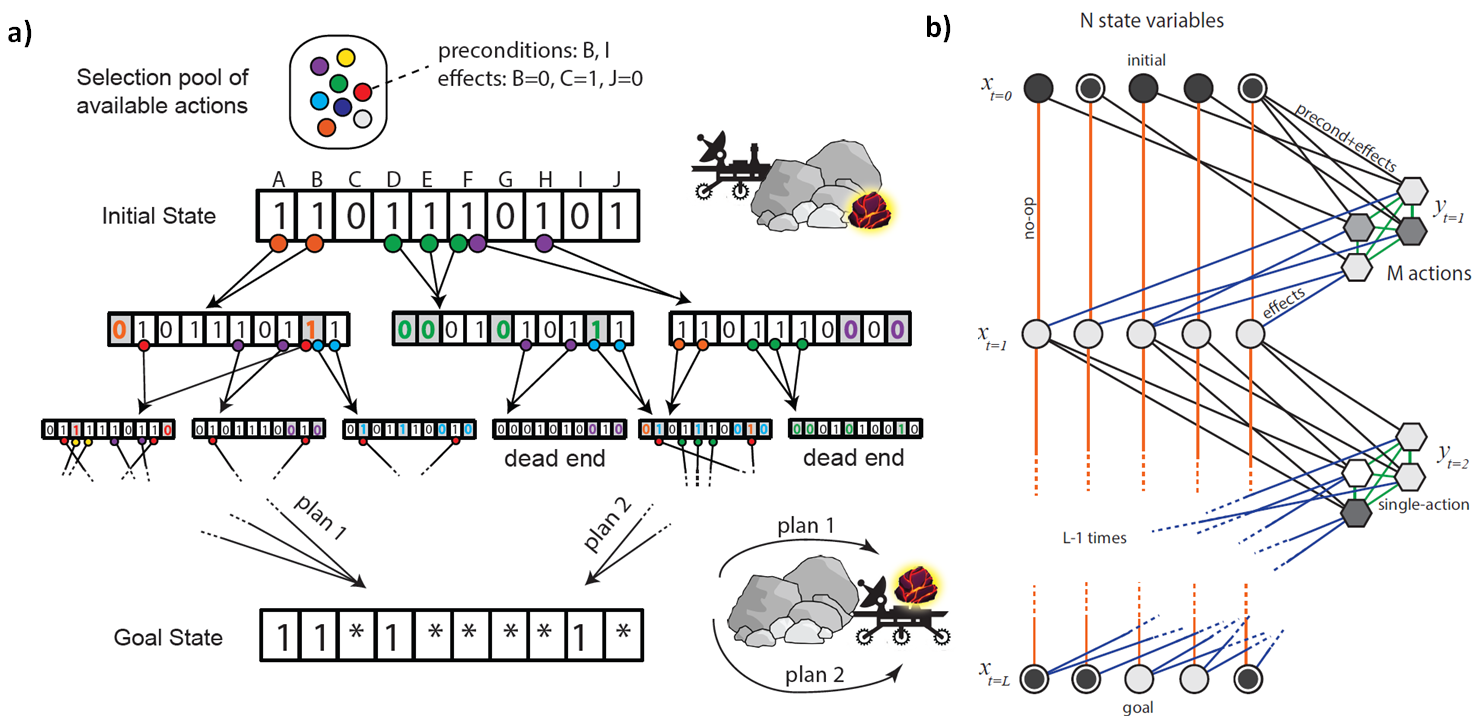
Figure 4: (a) Pictorial view of a planning problem. The initial state (e.g., Rover behind the rocks without sample) is specified by assigning True (1) or False (0) to state variables (named A-J in this simplified example). The planning software navigates a tree, where a path represents a sequence (with possible repetitions) of actions selected from a pool (colors). Each action has preconditions on the state variables (e.g., moves can be done around the rocks but not through them) that need to be satisfied for the actions to be executed (the circles under the state variables in the search tree need to be True) and has an effect on the state (colored variables in shaded regions of the new state have changed values). A valid search plan (multiple valid plans are possible) will reach the goal state (e.g., Rover in front of the rocks with a sample collected). (b) Direct time-indexed QUBO structure for a planning problem with only positive preconditions and goals. Each node represents a state variable (left) or an action (right) at any given time $t$. Time flows from top to bottom, and variables $y_{i}^{(t)}$ for the actions at time $t$ are shown between the state variables $x_{i}^{(t-1)}$ for one time step and the state variables $x_{i}^{(t)}$ for the next time step. The node grayscale intensity represents the magnitude of local field (bias) $h_{i}$ applied to a given qubit $i$, and the double contour in a node indicates a negative bias.

Ref. [5] discusses a general QUBO formulation of planning problems (see Fig. 4(b)). If the original planning problem has $N$ state variables and we are looking for a plan of length $L$, then the QUBO problem will have $N(L+1)$ binary variables $x_{i}^{(t)}$, where $t\in\{0,\dots,L\}$ is the time index, and $i$ is the index of the state variable in the original planning problem. In addition, if the original planning problem has $M$ possible actions, we will have $LM$ additional binary variables $y_{j}^{(t)}$ which indicate whether the $j$th action is carried out at time step $t$ or not. A QUBO can then be defined in terms of these variables, with terms capturing the goal, precondition, effect, single-action, and no-op (no variable change without an action) constraints:

$$H=H^{\prime}_{\operatorname{goal}}+H_{\operatorname{no}-\operatorname{op}}+H^{\prime}_{\operatorname{precond}}+H_{\operatorname{effects}}+H_{\operatorname{single-action}}.$$ (4)

Ref. [5] describes a somewhat more general cost function that supports multiple actions per time step.

4.1.2 Advanced scheduling applications

Scheduling was recognized early on as one the most promising near-term targets for quantum annealing due to its efficient quadratic time-indexed Mixed-Integer Linear Programming formulation. Furthermore, there is a rich literature of complex pre-processing and hybrid classical techniques. Using this direct quadratic formulation of scheduling instead of the most general planning formulation leads to very significant performance advantages in runs of the D-Wave machines [5].

Scheduling formalizes problems dealing with the optimal allocation of resources (machines, people) to tasks (jobs) over time, under various constraints and figures of merit. In one direct QUBO formulation, a bit is associated to the execution of a given job in a given machine (out of $M$ possible) at a given time (discretized in $T$ slots), allowing for very efficient mappings on current quantum annealers supporting two-body Ising-type interactions, using $NMT$ qubits, where $N$ is the number of jobs. While objective functions of the priority maximization type are easily implementable as linear penalty functions requiring only local fields on the corresponding logical bits, objectives requiring makespan minimization require a more involved encoding with either $T$ ancilla clock variables highly connected to the qubits relative to the jobs scheduled last, or by complementing the quantum solver with guidance from classical methods, such as binary search [12].

Many planning and scheduling problems are of such scale and complexity that they are by necessity solved in pieces, and so quantum hardware can be naturally integrated into the solution of such problems. Hybrid solvers employing quantum annealing together with classical methods are particularly suited to scheduling applications, because the state-of-the-art approaches for specific scheduling problems are typically combining different approaches in a modular way, and decompositions can be employed to get around programming bottlenecks such as high connectivity, precision requirements, continuous constraints, or to employ quantum annealing as a heuristic module of a complete solver [17, 18]. As a heuristic module of a complete solver, quantum annealing enables more directed search of the solution space. Building a complete solver out of a probabilistic quantum subroutine requires non-trivial classical co-processing, but recent work has shown that it can be done successfully. In particular, partial solutions returned by a quantum solver can be used to derive bounds on the optimum value of the function to be optimized, and therefore focus on the most promising or neglect the least promising parts of the solution space.

Recent work on the application of quantum annealing to scheduling includes programming and benchmarking quantum annealers on small problems from the domains of graph coloring [5], job shop scheduling [12], Mars lander activity scheduling [17], air traffic runway landing [18], and alternative resource scheduling [18]. The question of speedup with respect to purely classical methods are inconclusive due to the small size of the problems implementable on current quantum annealers and the inefficiency of embedding techniques [5]. This body of work has identified precision and connectivity requirements that suggest future generations of annealers may be able to solve currently intractable scheduling problems within a decade.

Planned technological advances in quantum annealing architectures will also make possible tighter integration of quantum and classical components in the hybrid approaches discussed above, both through more programmable devices that allow for greater flexibility as subroutines and through application-specific devices that maximize the effectiveness of particular algorithms. In future, we expect quantum hardware to be integrated into larger systems much as graphical processing units are today [19].

4.2 Fault detection and diagnostics of graph-based systems

Another application domain we have studied with quantum annealing devices is the diagnostics of electrical power-distribution systems (EPS); a collaboration between QuAIL and the Discovery and System Health (DaSH) technical area at NASA Ames. Diagnosing the minimal number of faults capable of explaining a set of given observations, e.g., from sensor readouts, is a hard combinatorial optimization problem usually addressed with artificial intelligence techniques. In [20], we presented the first application of the Combinatorial Problem $\rightarrow$ QUBO Mapping $\rightarrow$ Direct Embedding process where we were able to embed instances with sizes comparable to those found in real-world problems. We demonstrated problem instances with over 100 electrical components (including circuit breakers and sensors) running on a quantum annealing device with 509 quantum bits. In comparison, the number of components in the electrical circuits used for diagnostics competitions from NASA’s Advanced Diagnostics and Prognostics Testbed (ADAPT) ranges between 40 and 100 [21].

4.2.1 QUBO formulation

As shown in Fig. 5(a), there are two types of components. The first are circuit breakers (CB), which in their healthy mode allow the flow of current, and are illustrated as the nodes of the quaternary tree. We denote them by the set of binary variables $\{x_{i}\}$, with $x_{i}=1$ ($x_{i}=0$) corresponding to CB $i$ in a healthy (faulty) state. The other component type is the sensor or ammeter, which is not only another electrical component that could potentially malfunction, but also forms part of the observations from which one is asked to perform the diagnosis of the electrical network. Therefore, for each ammeter, we have an observation parameter and a status variable indicating its healthy or faulty state. The observations (or readouts) are part of the problem definition and provided as input parameters. We denote this set of binary parameters $\{l_{i}\}$, with $l_{i}=1$ ($l_{i}=0$) if the $i$-th ammeter is showing a High (Low) readout. Similar to the $\{x_{i}\}$ variables for the CBs, the uncertainty in the ammeter readouts is introduced by assigning to them a set of binary variables, $\{y_{i}\}$, with $y_{i}=1$ ($y_{i}=0$) corresponding to ammeter $i$ in a healthy (faulty) state.

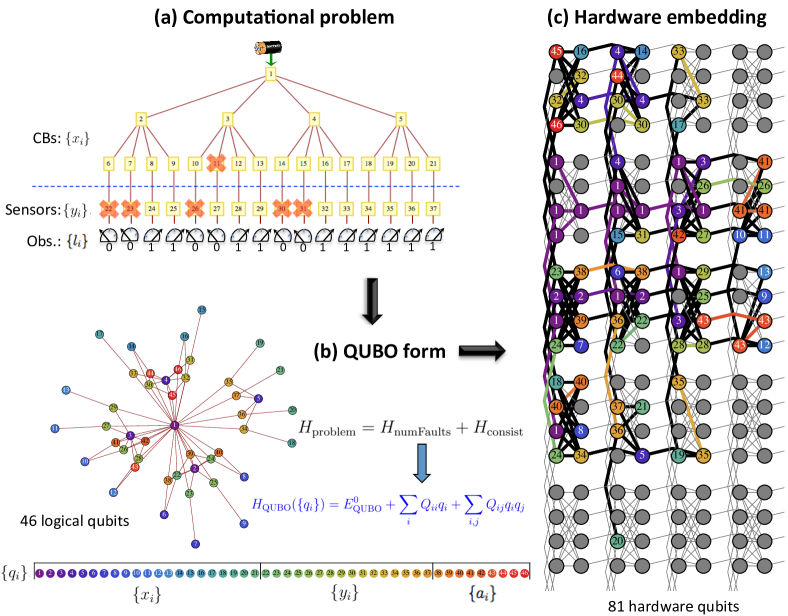
Figure 5: General scheme of an experimental setup for the diagnosis of multiple faults with a quantum annealer. (a) A possible realization of the diagnosis of multiple faults in an EPS network with one power source, 21 CBs and 16 sensors or ammeters. The orange crosses indicate faulty electrical components ($x_{i}=0)$. In this particular instance of 6 faults, a plausible explanation of the readouts places one of the faults on a CB and the remaining 5 on the ammeters. However, this is only one of the $2^{6}$ six-fault explanations that are equally likely in this case. (b) QUBO form of the problem where coupling between two logical qubits is represented as edges. (c) The subsequent embedding into the Chimera graph usually requires more variables since some logical qubits are represented by several physical qubits (depicted here as nodes in the graph) due to the sparse connectivity of the hardware graph. In this problem, 81 physical qubits are needed to implement the QUBO with 46 logical variables.

The goal is to find the minimum number of faults in the electrical components, either in the CBs and/or the ammeters, consistent with the circuit layout and the readouts. We solve this as a minimization problem over the pseudo-Boolean function $H_{\text{problem}}(\{x_{i}\},\{y_{i}\};\{l_{i}\})$, whose construction is explained below. After $H_{\text{problem}}$ is transformed into its QUBO form, we can subsequently use the quantum annealer to find the assignment for each of the $\{x_{i}\}$ and $\{y_{i}\}$.

The construction of the pseudo-Boolean function contains two contributions:

$$H_{\text{problem}}=H_{\text{numFaults}}+H_{\text{consist}}.$$ (5)

$H_{\text{consist}}$ is constructed such that it is 0 whenever the prediction from the assignment of all the $\{x_{i}\}$ and $\{y_{i}\}$ is consistent with the readouts $\{l_{i}\}$ from the ammeters, and greater than 0 when the readouts and the prediction, given the $\{x_{i}\}$ and $\{y_{i}\}$ assignments, do not match. Consider the set $P_{i}$ as the set of CB indices in the path from the root node (CB 1) where power is input, all the way to the CB connected to the $i$-th ammeter. Thus, for the network in Fig. 5(a), $P_{1}=\{1,2,6\}$, $P_{2}=\{1,2,7\}$, $\cdots$, and $P_{16}=\{1,5,21\}$. If we denote the number of paths as $n_{\text{paths}}$ (equals the number of ammeters in this network), one can construct $H_{\text{consist}}$ as:

$$H_{\text{consist}}=\lambda_{\text{path}}\sum_{i=1}^{n_{\text{paths}}}y_{i}g_{i},\quad f_{i}(\{x_{j}\}_{j\in P_{i}})=\prod_{j\in P_{i}}x_{j},$$ (6)

with $g_{i}=l_{i}+f_{i}-2f_{i}l_{i}$, a binary function with $g_{i}=0$ when the prediction $f_{i}$, based only on the CB statuses in the path $P_{i}$, is consistent with the readouts $l_{i}$, and $g_{i}=1$ when the prediction and the readout are in disagreement. In other words, $g_{i}=\textsc{xor}(f_{i},l_{i})$.

$H_{\text{numFaults}}$ is proportional to the number of faults (whenever $x_{i}=0$ or $y_{i}=0$) in the electrical network:

$$H_{\text{numFaults}}=\lambda^{\text{CB}}_{\text{faults}}\sum_{i=1}^{n_{\text{CB}}}(1-x_{i})+\lambda^{\text{sensor}}_{\text{faults}}\sum_{i=1}^{n_{\text{sensor}}}(1-y_{i}),$$ (7)

and when combined with $H_{\text{consist}}$, as written in Eq. (5), defines the problem energy function to be minimized by favoring the minimal set of faulty components that are simultaneously consistent with the observations in the outermost sensors. A thorough discussion on setting the values of all the penalties is provided in [20].

Notice the pseudo-Boolean $H_{\text{consist}}$ is a high-degree polynomial, and for this particular network, the order of the polynomial is related to the depth of the tree. We can reduce the degree of the polynomial to a quadratic expression, $H_{\text{QUBO}}$, with the overhead of adding more binary variables, while conserving the global minimum of the original function, $H(\{x_{i}\},\{y_{i}\};\{l_{i}\})$. Further details on the techniques used for this reduction are provided in [20, 22].

Assuming it requires $n_{A}$ ancilla variables $\{a_{i}\}$ to reduce the high-degree polynomial to the quadratic expression, we can relabel the CB, sensor, and ancilla variables, $\{x_{i}\}$, $\{y_{i}\}$, and $\{a_{i}\}$, respectively, into a new set of binary variables $\{q_{i}\}$ for $i=1,2,\cdots,n_{l}$, with $n_{l}=n_{\text{CB}}+n_{\text{sensor}}+n_{A}$ as the total number of logical qubits. The final quadratic cost function to be minimized can then be written as

$$\begin{split}H_{\text{QUBO}}(\{q_{i}\})&=E^{0}_{\text{QUBO}}+\sum_{i,j}Q_{i,j}q_{i}q_{j}\\ &=E^{0}_{\text{QUBO}}+\mathbf{q}^{T}\cdot\mathbf{Q}\cdot\mathbf{q}.\end{split}$$ (8)

As shown in Fig. 5, this expression can be represented as a graph with the number of vertices equal to the number of logical qubits $n_{l}$ corresponding to the set of variables $\{q_{i}\}$. In this representation, $Q_{i,i}$ can be treated as the weights on the vertices, while $Q_{i,j}$ are the weights for the edges representing the couplings between variables $i$ and $j$ (see Fig. 5). Notice that since $q^{2}_{i}=q_{i}$, the expression $\mathbf{q}^{T}\cdot\mathbf{Q}\cdot\mathbf{q}$ contains both linear terms $Q_{i,i}$, and quadratic terms, $Q_{i,j}$, when $i\neq j$. $E^{0}_{\text{QUBO}}$ corresponds to the constant independent term.

Although the problems studied in [20] are simpler than typical real-world instances, we believe that they still capture some non-trivial features, such as the inclusion of uncertainty in the sensor readouts. Of course, aiming to embed all the details from realistic scenarios will require significantly more qubits and also depend on the specific network/problem to be solved.

As another realization of the fault detection application, the QuAIL team is examining combinational digital circuits [23], a more realistic scenario used to benchmark codes devoted to solving diagnostics related problems [21]. Preliminary results look very promising and harder than any other benchmarks reported in the literature and used to address the question of quantum speedup in quantum annealers.

4.3 Sampling and machine learning applications

Sampling from high-dimensional probability distributions is at the core of a wide spectrum of computational techniques with important applications across science, engineering, and society. Examples include deep learning, probabilistic programming, and other machine learning and artificial intelligence applications.

Much of the record-breaking performance of classical machine learning algorithms regularly reported in the literature pertains to task-specific supervised learning algorithms [24]. Unsupervised learning algorithms are more human-like, and in principle more general and powerful, but their development has been lagging due to the intractability of traditional sampling techniques such as Markov Chain Monte Carlo (MCMC). Indeed, as leading researchers in the field have pointed out [24], future success of unsupervised learning algorithms requires breakthroughs in efficient sampling algorithms. Quantum annealing holds the potential to sample more efficiently and from more complex probabilistic models, which would significantly advance the field of unsupervised learning.

4.3.1 A different class of problems for quantum annealing

A computationally hard problem, key for some relevant machine learning tasks, is the estimation of averages over probabilistic models defined in terms of a Boltzmann distribution

$$P_{B}(\mathbf{s})=\frac{1}{Z}\mathop{\mbox{exp}}\left({\sum_{i,j}W_{ij}s_{i}s_{j}+\sum_{i}b_{i}s_{i}}\right),$$ (9)

where $Z$ is the normalization constant or partition function, $\mathbf{s}=\{s_{1},\dots,s_{N}\}$ denotes a configuration of binary variables, and $W_{ij}$ and $b_{i}$ are the parameters specifying the probability distribution.

Sampling from generic probabilistic models, such as $P_{B}(\mathbf{s})$ in Eq. (9), is hard [25] in general. For this reason, algorithms relying heavily on sampling are expected to remain intractable no matter how large and powerful classical computing resources become. Even though quantum annealers were designed for challenging combinatorial optimization problems, it has been recently recognized as a potential candidate to speed up computations that rely on sampling by exploiting quantum effects, such as quantum tunneling  [26, 27].

4.3.2 Quantum-assisted learning of Boltzmann machines

Indeed, some research groups have recently explored the use of quantum annealing hardware for the learning of Boltzmann machines and deep neural networks (see [26, 28] and references therein). The standard approach to the learning of Boltzmann machines relies on the computation of certain averages that can be estimated by standard sampling techniques, such as MCMC. Another possibility is to rely on a physical process, like quantum annealing, that naturally generates samples from a Boltzmann distribution. In contrast to their use for optimization, when applying quantum annealing hardware to the learning of Boltzmann machines, the control parameters (instead of the qubits’ states) are the relevant variables of the problem. The objective is to find the optimal control parameters that best represent the empirical distribution of a given dataset.

These ideas are framed within a hybrid quantum-classical computing paradigm. Given a classical machine learning infrastructure, the idea is to replace the software module that generate samples, e.g., via MCMC, with a quantum annealing process. This quantum sampling module could be similarly employed in other domains where sampling is useful. Thus, demonstrating quantum speedup for sampling would have broad implications.

In recent work [26], the QuAIL team has demonstrated how to properly use a quantum annealer by overcoming critical challenges such as the instances-dependent temperature estimation. In fact, while the probability distribution $P_{B}(\mathbf{s})$ in Eq. (9) is specified by parameters $W_{ij}$ and $b_{i}$, the control parameters of a quantum annealer are instead $J_{ij}=T_{\rm eff}\,W_{ij}$ and $h_{i}=T_{\rm eff}\,b_{i}$. According to quantum dynamical arguments [27], $T_{\rm eff}$ is an instance-dependent effective temperature, different from the physical temperature of the device. Unveiling this unknown temperature is key to effectively using a quantum annealer for Boltzmann sampling. By introducing a simple effective temperature estimation algorithm [26], it was possible to successfully use the D-Wave 2X system for the learning of a special class of restricted Boltzmann machines that can serve as a building block for deep learning architectures. Experiments run using a synthetic dataset showed that the quantum-assisted algorithm outperformed in terms of quality (i.e., the value of the likelihood reached) the standard classical algorithm named CD-1 and approached the performance of CD-100, which takes about 100 times more computational effort than CD-1 (See [26] for details). Complementary work that appeared roughly simultaneously showed that quantum annealing can be used for supervised learning in classification tasks [28].

These results are encouraging, but there remain numerous challenges before the full potential of quantum annealing hardware for sampling problems can be harnessed. While each future generation will no doubt be an improvement, hardware advances alone will not suffice. The QuAIL team is therefore developing algorithmic strategies to address these other problems, with promising initial results. For example, we recently experimentally demonstrated [29] the feasibility of a fully unsupervised machine learning application by successfully training our quantum annealer, using up to 940 qubits, to generate, reconstruct, and classify images that closely resemble (low resolution) handwritten digits, among other synthetic datasets. We showed a Turing test (see Fig. 4 in [29]) to challenge people to distinguish between handwritten digits and digits generated by the quantum device; most people we informally showed this Turing test either failed or found it difficult. To reach this milestone, we implemented densely connected hardware-embedded models that are more robust to noise and more efficient to learn with state-of-the-art quantum annealers.

The ultimate question that drives this endeavor is whether there is quantum speedup in sampling applications. Current experience with the use of quantum annealers for combinatorial optimization suggest the answer is not straightforward. This work is part of the emerging field of quantum machine learning [30], an essentially unexplored territory where quantum annealing might have a large impact in the near term.

4.4 Best practice programming and compilation techniques

These explorations have spurred QuAIL to design advanced techniques to guide programming and improve performance. Software calibration methods devised by the team are described in [31]. In [5], we compare different mappings and in [32], we present advanced techniques to intelligently select gauges based on small numbers of trial runs that often improve performance by an order of magnitude. Compilation strategies for quantum annealers, including guidelines for optimally setting the strength of $J_{F}$ are discussed in [5, 11, 12]. Furthermore, we have identified certain common structures in the QUBO representations of many applications because different constraints often have similar forms [5].

5 Physics of quantum annealing

This section discusses results clarifying the role of various processes in quantum annealing that suggest where to look for potential quantum speedup and where such an advantage would be unlikely. So far, we have been informal about what we mean by quantum speedup. However, knowing the different types of quantum speedup is helpful in assessing results related to the computational power of quantum annealing. It is also necessary to improve our understanding of potential classes of problems for which such a quantum device can excel.

5.1 Background on quantum annealing

The target of quantum annealing is to optimize a function of QUBO form, as in Eq. (1). The cost function has a physical realization in a system comprising quantum bits (qubits) where each binary variable is encoded as a qubit. The coefficients ($a_{i}$) translate into bias fields applied on the qubits and ($b_{i,j}$) is represented as the coupling strength between two qubits. The cost function thus corresponds to a Hamiltonian, $H_{1}$, as in Eq. (2), which describes the energy of the system. The Hamiltonian bears strong similarity with the cost function. However, while in the classical cost function the binary variables can take value either 0 or 1, in a Hamiltonian the qubit is allowed to be (and in a physical quantum system, can be) in a superposition of these two states $\alpha|0\rangle+\beta|1\rangle$. The optimization problem translates into finding the ground state of the Hamiltonian, i.e., the eigenstate of the lowest eigenvalue of $H_{1}$. In order to do so, quantum annealing introduces quantum fluctuation in the system, represented as a non-commuting term in the Hamiltonian, $H_{0}$. A typical $H_{0}$ easy to prepare physically is $H_{0}=\sum_{j}\sigma^{x}_{j}$ where each $\sigma^{x}_{j}$ swaps states $0$ and $1$ on the $j$-th qubit. The weight of $H_{0}$ with respect to $H_{1}$ is the strength of the fluctuation. The initial state of the system is one with all possible classical configurations that are equally likely. The system starts with a strong quantum fluctuation that gradually quenches. The quantum fluctuation provided by $H_{0}$ allows the dynamics to explore a larger region of the search space and gradually concentrate (with large probability) at the global minimum. At the beginning of the search, the initial state is very far from the global minimum but a large fluctuation allows the system a better chance to accept a state that is energetically higher; thus allowing a more extensive search of the solution space. As the annealing progresses, the fluctuation is tuned down and the system spends more and more time around the global minimum, eventually staying there once the fluctuation disappears. This process resembles simulated annealing where the quantum fluctuation replaces the thermal fluctuations.

Another perspective of the same process is to view the total Hamiltonian as slow moving and time dependent. If the Hamiltonian is varying slowly enough, the system will follow its instantaneous eigen-state (this is known as the adiabatic theorem). Since the initial state is actually the ground state of $H_{0}$, a slow tuning would eventually result in the ground state of the problem Hamiltonian, $H_{1}$. A key question is: how slow is slow enough? During the evolution when there is another energy level close to the ground state and if the change of Hamiltonian is not slow enough, there is a risk the system would jump to the higher level and never return, and the algorithm would fail. The closer the two energy levels are, the slower the Hamiltonian must vary in order to mitigate this risk. The spectral gap (the minimal distance between the two energy levels) plays a crucial role in quantum annealing.

Ref. [33] defines four classes of quantum speedups:

• Provable quantum speedup: It is rigorously proven that no classical algorithm can scale better than a given quantum algorithm.

• Strong quantum speedup: The quantum heuristic is faster than any known classical algorithm. This type of speedup has been established for dozens of special-purpose algorithms, with Shor’s polynomial-time algorithm for factorization being the most prominent. The best classical algorithm may be continually evolving, as is the case for most areas in which classical heuristics prevail; the ICAPS (International Conference on Automated Planning and Scheduling) planning competition and the SAT competition generally see new algorithms every year.

• Potential quantum speedup: The quantum speedup is in comparison to a specific classical algorithm or a set of classical algorithms.

• Limited quantum speedup: There is a quantum speedup only if the quantum heuristic is compared to the closest classical counterpart.

A finer-grained classification, which takes into account the type of classical algorithm used in the comparison, has been proposed in [34].

To better understand where quantum annealing may confer an advantage, it is important to appreciate its major sources of error. The algorithm may fail to find a solution due to escape from the ground state via either non-adiabatic transitions or decoherence processes. Yet another possibility is that the ground state does not correspond to the optimal solution due to control noise. In the following, we review some of the recent developments in assessing the impact of these error mechanisms.

5.2 Quantum annealing bottlenecks

Some insight into the relative performance of quantum annealing can be gained by studying random optimization problems using the tools of the the statistical mechanics. Absent noise, non-adiabatic transitions can be prevented only if the annealing proceeds slowly across points where the gap $\Delta E$ that separates the instantaneous ground state from excited states becomes small (taking at least time $t\propto\hbar/\Delta E$). The most widely discussed bottleneck, where the gap reaches a local minimum, is the quantum phase transition. Some of the computationally hardest problems exhibit a discontinuous (first order) phase transition, where the gap is exponentially small. In a common scenario, the ground state wavefunction abruptly changes from being a superposition of a large number of spin configurations to being nearly localized near a global minimum. If the transverse field is lowered too fast, the algorithm performs no better than a random guess.

Continuous (second order) phase transitions scale better, although strong fluctuations of disorder (randomness of the parameters of the problem) can still make the gap scale as a stretched exponential (exponential in some fractional power of problem size). This still leaves a large swath of problems — most amenable to quantum annealing — where the disorder is irrelevant at the critical point (phase transition) so that the gap there is only polynomially small. Recent work [35] addresses this practically relevant scenario and finds that after the phase transition bottleneck, the algorithm encounters further bottlenecks with gaps that scale as a stretched exponential.

As annealing progresses, the number of spin configurations with significant amplitudes decreases until the wavefunction is completely localized. This is roughly equivalent to having a partial assignment of variables: An increasing fraction of binary variables have converged to a definite value, while the remaining variables are in a superposition state. At times, a state with a different assignment of already fixed variables becomes more energetically favorable, and a large number of variable have to flip simultaneously in a multi-qubit tunneling, which is the source of ”hard” bottlenecks described above. This process is analogous to ”backtracking” in classical search algorithms.

The major finding is that the number of tunneling bottlenecks is proportional to the logarithm of problem size. In practice, as the problem size increases, the time complexity of quantum annealing will exhibit a crossover from polynomial scaling (when the phase transition bottleneck is dominant) to exponential (when the expected number of ”hard” bottlenecks exceeds one). This size threshold is related to the ”density” of spin glass bottlenecks. Similar concept can be introduced for other heurstic search algorithms, such as simulated annealing. The bottleneck density can thus be used as a metric of performance indicating problem sizes above which the time complexity increases exponentially.

Interestingly, the minimum requirement for the annealing time is to avoid non-adiabatic transition at the phase transition (polynomial scaling). As it turns out, for fully coherent annealing, having one long annealing cycle versus choosing the best out of repeated short cycles results in identical time-to-solution (as long as annealing time exceeds the aforementioned minimum). Shorter annealing times minimize the effects of decoherence and have been favored in most experimental studies on the D-Wave hardware.

Coupling to the environment affects these results in multiple ways. First, it changes the universality class of the phase transition, worsening scaling of the minimum annealing cycle [36]. Second, it suppresses multi-qubit tunneling since in addition to flipping qubits, corresponding environmental degrees of freedom have to adjust. If quantum-mechanical tunneling is strongly suppressed, equilibrium may be reached via thermal excitation due to finite temperature. In this regime, performance would paradoxically improve with increasing temperature as the system becomes more classical.

5.3 Multi-qubit co-tunneling

Multi-qubit quantum co-tunneling is expected to be a key microscopic mechanism responsible for quantum speedup in quantum annealing. In the following, we consider limited speedup; i.e., speedup compared to simulated annealing. Realistic hardware is subject to intrinsic noise that affects the quantum dynamics of the system, and therefore needs to be considered when evaluating the efficiency of quantum annealing hardware. The effect of hardware noise is twofold: (1) Coupling to noise allows inelastic processes, prohibited by energy conservation in the closed system. Inelastic relaxation provides an efficient route to a local minimum within a convex region of the potential energy landscape. (2) Dephasing noise leads to loss of coherence between the states on different sides of the barrier, resulting in an incoherent tunneling regime, and, in the strong coupling regime, causes renormalization of the tunneling rate.

In the case of the flux qubits of the D-Wave system, the typical decoherence time (a measure of how long quantum features of a single qubit can be maintained, specifically the characteristic decay time of the off-diagonal elements of the qubit’s density matrix) is of the order of nanoseconds to tens of nanoseconds, which is shorter than the minimum run time of the annealing schedule, 5 microseconds. Nevertheless, D-wave annealers demonstrate signatures of quantum many-body dynamics, particularly incoherent multi-qubit quantum tunneling and evidence of 8-qubit tunneling has been reported [37]. In the course of quantum annealing, the dynamics of the device is limited to low-energy multi-qubit superposition states, which are more robust against the effects of noise and decoherence than single qubit states. In this regime, single qubit excitations caused by noise local to each qubit are strongly suppressed by the strong qubit-qubit coupling energy. At the same time, slow fluctuations of local magnetic flux result in a time-dependent spectrum of the multi-qubit low-energy states, which introduces decoherence of the multi-qubit dynamics.

In the vicinity of the algorithm’s bottlenecks, quantum annealing hardware realizes incoherent tunneling [37]. Different tunneling regimes are determined by comparing the quantum tunneling rate near the computational bottleneck to the characteristic dephasing rate. In a common regime, the tunneling rate near the bottleneck is exponentially small, while the dephasing rate is at least of order one. In this regime, quantum tunneling can be only incoherent in nature [38]: an analog of the decay of a metastable state into a continuous spectrum encountered in nuclear physics and chemistry, as opposed to a coherent superposition of states on two sides of a potential barrier. The incoherent regime is characterized by a quadratic slowdown of quantum tunneling. Nevertheless, there exist classes of problems where limited polynomial speedup is possible in this regime, particularly in cases where the shape of the potential barrier favors quantum tunneling over classical over-the-barrier escape, such as when barriers are tall and thin [39].

An alternative [40], operational also in the case of thick barriers where the usual intuition would favor classical escape, is the class of problems characterized by exponential degeneracy of the metastable state separated by a barrier from the global minima. The latter is typical for NP-hard problems; a common feature of classical mean-field spin glass models [41] is a polynomial number of the global minima separated by large potential barriers from an exponential number of metastable states. In such a landscape, simulated annealing slows down exponentially due to an additional entropic barrier associated with escaping the exponentially degenerate set of metastable states. In contrast, in the course of quantum annealing, the transverse field splits the degeneracy of the classical problem and thereby avoids the additional entropic barrier.

To better understand multi-qubit tunneling processes, we developed an instantonic calculus for analytical treatment of the thermally-assisted tunneling decay rate of metastable states in fully-connected quantum spin models [42, 43]. The tunneling decay problem can be mapped onto the Kramers escape problem of a classical random dynamical field. This dynamical field is simulated efficiently by path integral Quantum Monte Carlo (QMC). We show analytically that the exponential scaling with the number of spins of the thermally-assisted quantum tunneling rate and the escape rate of the QMC process are identical [44]. This analytical result complements prior numerical work [45] and provides an explanatory model. This effect is due to the existence of a dominant instantonic tunneling path. We solve exactly the nonlinear dynamical mean-field theory equations for a single-site magnetization vector that describe this instanton trajectory. We also derive scaling relations for the “spiky” barrier shape when the spin tunneling and QMC rates scale polynomially with the number of spins while a classical over-the-barrier activation rate scales exponentially.

5.4 Role of noise

Intrinsic noise cannot be eliminated from real quantum devices: manufacturing imperfections, as well as thermal fluctuations, induce quantum dephasing and decoherence (see Section 6). Noise can sometimes be helpful (thermal fluctuations are responsible for the thermally-assisted annealing effects discussed earlier), but can cause quantum devices to work far from their ideal state, limiting the actual performance and hiding any potential quantum speedup.

In addition, control noise can change the target Hamiltonian $H_{1}$ with the consequence that the target solution is no longer in the ground subspace of $H_{1}$. In this case, even a perfect quantum device, subject only to control noise, would find a “false” ground state, which could be far from any target solution. The maximum noise that can be added to $H_{1}$ before the target solutions do not belong to the ground subspace of $H_{1}$ is called resilience [46, 47]. In general, resilience can be increased by properly rescaling the energy of $H_{1}$. Real quantum devices, however, have a limited range of energies so the resilience cannot be completely neglected. Recent work shows that a low resilience could hide a quantum speedup [46].

6 Quantum annealing hardware

To date, the most significant progress in quantum annealing hardware is based on the engineering of quantum superconducting circuits with macroscopic collective variables (e.g., electric charge and magnetic flux) exhibiting quantum coherence. Here we review basic design and operational principles of such circuits, focusing on different types of superconducting qubits, inter-qubit coupling, and decoherence processes caused by various sources of the environmental noise.

6.1 Quantization of electric circuits with Josephson junctions

Let us briefly describe quantization of zero-resistance superconducting circuits, which is based on the lumped element method [48, 49, 50]. We can represent a circuit using two alternative sets of variables: current and voltage ($I(t)$ and $V(t)$) or charge and flux ($Q(t)$ and $\Phi(t)$), connected with each other via the relations $I=dQ/dt$ and $V=d\Phi/dt$. Let us start with the simplest circuit such as an LC oscillator (see Fig. 6(a)), whose dynamics is governed by the Kirchhoff’s laws $I_{L}=I_{C}\equiv I$ and $V_{L}+V_{C}=0$. Using $V_{L}=LdI/dt$ and $V_{C}=Q_{C}/C$, one obtains the equation of motion $\ddot{I}+\omega_{LC}^{2}I=0$, where $\omega_{LC}=1/{\sqrt{LC}}$ is the characteristic frequency for classical current (and voltage) oscillations. The magnetic flux $\Phi$ and charge $Q$ are governed by similar equations, e.g., $\ddot{\Phi}+\omega_{LC}^{2}\Phi=0$. Using variables $(Q,\Phi)$ one can express the equations of motion in the Hamiltonian form, $\dot{\Phi}=\partial H/\partial Q$ and $\dot{Q}=-\partial H/\partial\Phi$, where the classical Hamiltonian function is $H=Q^{2}/2C+\Phi^{2}/2L$. Following the standard quantization procedure, we replace classical variables with corresponding operators, introduce the commutator $\left[{\hat{\Phi},\hat{Q}}\right]=i\hbar$, and arrive at the Hamiltonian of a quantum harmonic oscillator, $\hat{H}=\hat{Q}^{2}/2C+\hat{\Phi}^{2}/2L$, describing the quantized electromagnetic modes of a macroscopic LC circuit with equidistant energy levels, $E_{n}=\hbar\omega_{LC}(n+1/2)$ with $n=1,2\ldots$. Clearly, this energy spectrum is not suitable for an implementation of a two-level qubit.

-

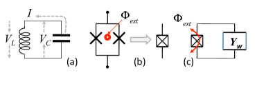
Figure 6: (a) Lumped element model for LC oscillator with current $I$ and voltages $V_{C}=-V_{J}$. (b) Tunable SQUID loop biased by external flux $\Phi_{ext}$. (c) Effective circuit of a qubit.

In order to separate two well-defined levels that can be used as logical states $|0\rangle$ and $|1\rangle$, one should employ a non-harmonic circuit with almost negligible coupling of the qubit levels and the rest of the spectrum. A natural solution is to introduce a Josephson junction as a nonlinear and non-dissipative element of the circuit. Josephson junctions are formed by two superconductors weakly connected through a high barrier. Within the lumped element approach, they are described by the current-voltage characteristics $I_{J}=I_{0}\sin(2\pi\Phi/\Phi_{0})$ where $I_{0}$ is a critical current and $\Phi_{0}=\pi\hbar/e$ is the flux quantum. Analysis of different realizations of a qubit is based on the Kirchhoff’s laws and on the description of the junction’s contributions in terms of $I_{J}$ and $V_{J}$ (or $\Phi$).

A tunable qubit is realized if one replaces a single Josephson junction by a SQUID loop formed by two parallel junctions biased by an external flux, $\Phi_{ext}$ (see Fig. 6(b)). The current passing through the SQUID is given by $I_{J}=I_{0}\cos(2\pi\Phi_{ext}/\Phi_{0})\sin(2\pi\Phi/\Phi_{0})$ [51], which can be thought of as an effective junction with tunable critical current $I_{\text{eff}}=I_{0}\cos(2\pi\Phi_{ext}/\Phi_{0})$ controlled by $\Phi_{ext}$. A typical tunable qubit can be represented as an effective junction shunted by a linear circuit with admittance $Y_{\omega}$ (see Fig. 6(c)). Below we consider two basic types of such qubits shunted by either LC oscillator (flux qubit) or a capacitor (charge qubit).

6.2 Hamiltonians of flux and charge qubits

Effective Josephson junctions, inductance and capacitance, connected in parallel, form a flux qubit (see Fig. 7(a)). The circuit is governed by the Kirchhoff’s laws for currents $I_{J,L,C}$ and voltages $V_{J,L,C}$: $I_{J}=I_{C}+I_{L}$, $V_{J}+V_{C}=0$, and $V_{J}+V_{L}=0$. Using these relations, we obtain the equation of motion for a flux $\Phi$ threading through the device as: $C{{\ddot{\Phi}}}+{{\Phi}}/{L}+I_{\text{eff}}\sin\left(\frac{{2\pi\Phi}}{{\Phi_{0}}}\right)=0$, which leads to the following Hamiltonian of a flux qubit

$$\hat{H}=\frac{\hat{Q}^{2}}{2C}+\frac{{(\hat{\Phi}-\Phi_{x})^{2}}}{{2L}}-\frac{{\Phi_{0}I_{\text{eff}}}}{{2\pi}}\cos\frac{{2\pi\hat{\Phi}}}{{\Phi_{0}}}~{}.$$ (10)

Here we assumed that the inductance loop $L$ can be biased by an additional external flux $\Phi_{x}$ applied through inductive coupling. The first (capacitance) term $\hat{Q}^{2}/2C$ in Eq. (10) can be interpreted as a kinetic energy while the second and third terms describe a potential formed by inductance and Josephson terms, respectively.

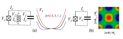
Figure 7: Effective circuits and potential energies vs. flux for: (a) Flux qubit (tunable Josephson junction shunted by LC oscillator); and (b) Junction shunted by capacitor only (charge qubit).

For further consideration, it is convenient to introduce dimensionless flux $\hat{\phi}=2\pi\hat{\Phi}/\Phi_{0}+\pi$ and charge operators $\hat{q}=-id/d\hat{\phi}$. Then the Hamiltonian in Eq. (10) can be expressed as

$$\hat{H}=4E_{C}\hat{q}^{2}+E_{L}\frac{(\hat{\phi}-\phi_{x})^{2}}{2}+E_{J}^{\text{eff}}\cos\hat{\phi},$$ (11)

and it is different from the LC oscillator by adding the effective energy of Josephson junction, $E_{J}^{\text{eff}}=\Phi_{0}I_{\text{eff}}/2\pi$. We also introduce here the capacitance and inductance energies, $E_{C}=e^{2}/2C$ and $E_{L}=(\Phi_{0}/2\pi)^{2}/L$ and $\phi_{x}=2\pi\Phi_{x}/\Phi_{0}+\pi$. The Hamiltonian in Eq. (11) corresponds to a particle with kinetic energy proportional to $E_{C}$ and potential energy determined by the interplay between $E_{L}$ and $E_{J}^{\text{eff}}$ through the ratio $\beta=E_{J}^{\text{eff}}/E_{L}=2\pi I_{\text{eff}}L/\Phi_{0}$. If $\beta<1$, Eq. (11) describes a single-well anharmonic oscillator, while for $\beta>1$ the double-well potential emerges and there are two closely-spaced tunnel-split levels defining a qubit. The quantum dynamics is determined by tunneling between the wells that can be controlled by variation of the barrier height $E_{J}^{\text{eff}}$, and by tilting the two-well potential via the tilt flux $\phi_{x}$. Flux qubits described by Eq. (11) are implemented in D-Wave quantum annealers [51].

A typical charge qubit operates as an open circuit shown in Fig. 7(b). To derive the Hamiltonian we must omit the inductance term in the equations of motion, which results in

$$\hat{H}=4E_{C}\hat{q}^{2}+E_{J}^{\text{eff}}\cos\phi,$$ (12)

and contains only the Josephson (periodic) part of the potential energy. The eigenvalue problem is reduced to the Mathieu equation. Operational regimes of various qubits described by the generic Hamiltonian in Eq. (12) drastically depend on the ratio $E_{J}/E_{C}$.

Several types of qubits have been realized during the last two decades. The simplest charge qubit, comprised of a voltage source in series with a Josephson junction (the Cooper pair box), had been implemented in [52]. Because of the large charging energy, $E_{J}/E_{C}\ll 1$, the two charge states different by a single Cooper pair are the working states of this qubit. Unfortunately, the Cooper pair box is highly sensitive to the charge noise. To overcome this difficulty, another qubit called the transmon was developed [53]. The transmon is derived from the Cooper pair box, but it operates in a different regime of $E_{J}^{\text{eff}}/E_{C}\gg 1$. It benefits from the fact that its charge dispersion and noise sensitivity decreases exponentially with $E_{J}/E_{C}$. Tuning $E_{J}^{\text{eff}}$ controls the amplitude of the potential, which forms a periodic array of minima and maxima shown as red and blue regions of a contour plot in Fig. 7(b). Since $E_{J}/E_{C}\gg 1$, tunneling between different minima is greatly suppressed and the qubit is realized at an arbitrary minimum where the lower states are unevenly spaced due to the nonparabolicity of the cosine potential. Therefore, one can manipulate the lowest pair of levels as in the case of a flux qubit. In Fig. 8, we present basic types of qubits [54] and show typical ratios $E_{L}/E_{J}$ and $E_{J}/E_{C}$ for these qubits (“Mendeleev-like table”) [55]. Selection criteria among various qubits for particular applications are determined not only by internal device parameters but also by their coupling properties and tolerance to the environmental noise.

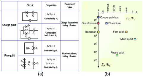
Figure 8: (a) Summary of the basic types of superconducting qubits [54]. (b) Ratios of energies $E_{L}/E_{J}$ and $E_{J}/E_{C}$ for different types of qubits (Mendeleev-like table) [55].

6.3 Inter-qubit coupling

Controllable couplings between qubits is at the heart of any quantum computing application. The simplest and most commonly used couplers are based on linear superconducting circuits; e.g., mutual inductances or capacitances, as shown in Figs. 9(a) or 9(b). A typical multi-qubit system is described by an anisotropic Heisenberg Hamiltonian: $\hat{\cal H}=\sum_{i,\alpha}B_{i\alpha}\hat{\sigma}_{i\alpha}+\sum\limits_{i,j,\alpha(i\neq j)}J_{ij}^{\alpha}\hat{\sigma}_{i\alpha}\hat{\sigma}_{j\alpha}$, where $\hat{\sigma}_{i\alpha}$ are pseudo-spin Pauli matrices in a qubit $2\times 2$ Hilbert space, $B_{i\alpha}$ are the components of local fields, and $J_{ij}^{\alpha}$ are exchange coupling parameters. Mechanism of inductive coupling between flux qubits $i$ and $j$ via mutual inductance $M_{ij}=M_{ji}$ (Fig. 9(a)) is straightforward: if $M_{ij}\neq 0$, the external flux from qubit $i$ threads through qubit $j$ loop (or vice versa) and affects the energy levels. Thus, the longitudinal coupling (proportional to $\hat{\sigma}_{1z}\hat{\sigma}_{2z}$) can be expressed as $J_{ij}^{z}\sim M_{ij}I_{i}I_{j}$. The direct inductive coupling is not tunable; however, a tunable coupling strength can be realized if the inductance loop is driven by a SQUID. An example of such coupling, utilized in D-Wave quantum annealers, is schematically shown Fig. 9(b) [56]. It is based on bias currents that produce controlled flux biases.

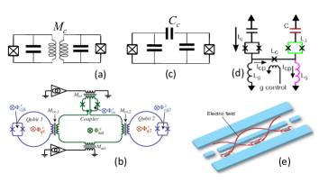
Figure 9: Effective circuits for different regimes of interqubit coupling: (a) between flux qubits via mutual inductance $M_{c}\equiv M_{12}$, (b) through inductive loop controlled by SQUID, [56] (c) between transmons coupled via capacitance $C_{c}$, and (d) tunable coupling between transmons controlled by Josephson junction with nonlinear inductance $L_{c}$. [57] (e) Schematic of the coplanar waveguide resonator (light blue), the transmon qubits and the first harmonic of the standing wave electric field shown in red. [58, 54]

A circuit diagram of two capacitively-coupled transmons is shown in Fig. 9(c), and can be analyzed using the lumped element method as above. As a result, the interaction Hamiltonian for a pair of transmons can be expressed as $\hat{q}_{i}\hat{q}_{j}C/C_{c}$. Calculating matrix elements of $\hat{q}_{i,j}$ within the two-level approximation, we obtain the transverse coupling (proportional to $\hat{\sigma}_{ix}\hat{\sigma}_{jx}$) with the coupling parameter $J_{ij}^{x}\sim\sqrt{\Delta E_{i}\Delta E_{j}}(C/C_{c})$, where $\Delta E_{i}$ is level splitting of $i$-th transmon. The purely capacitive coupling is not tunable, but the coupling strength can be controlled using a non-linear coupler with Josephson junction (a tunable inductor). This circuit is depicted in Fig. 9(d), where arrows indicate the flow of current for an excitation in the left qubit [57]. It is important that the coupling be tunable with nanosecond resolution, making this circuit suitable for various applications ranging from quantum logic gates to quantum simulations. Similar circuits are employed for readout of a flux qubit state in D-Wave quantum annealers, where each qubit is connected inductively with a quantum flux parametron ($rf$-SQUID with a small inductance, a large capacitance and a very large critical current) [51, 59]. Another approach is to couple all qubits to a shared passive element (quantum bus) such as a cavity or a coplanar waveguide resonator (CPW) [54].

6.4 Qubit relaxation and decoherence

Superconducting qubits are macroscopic quantum objects whose generic quantum properties, such as superposition of states and entanglement, inherently suffer from detrimental effects caused by a macroscopic, noisy environment [60]. To describe environmental noise phenomenologically, one should take into account random charge, flux, and Josephson junction noise sources that modulate lumped elements of the equivalent circuit in the qubit Hamiltonians in Eqs. (11) or (12).

After tracing over the environmental variables, the qubit dynamics is governed by the Bloch equation with two transition rates $\Gamma_{1}$ and $\Gamma_{2}$ (or times $T_{1}$ and $T_{2}$) describing qubit relaxation and decoherence, respectively. The two rates are related: $\Gamma_{2}=\Gamma_{1}/2+\Gamma_{d}$, where $\Gamma_{d}$ describes dephasing due to the low frequency noise. The flux qubits (e.g., D-Wave qubits) studied to date suffer from a low-frequency flux noise due to environmental spins [61, 62]. This leads to a substantial dephasing rate $\Gamma_{d}$ and, in turn, to a large difference between the relaxation and decoherence rates, $\Gamma_{2}\sim\Gamma_{d}\gg\Gamma_{1}$. In transmon qubits, the flux noise is absent and the low-frequency charge noise is suppressed; i.e., the decoherence rate is low and $\Gamma_{2}$ and $\Gamma_{1}$ are close to each other.

A particular choice of a qubit depends on its suitability for a given application. For instance, quantum annealing requires strong coupling between the qubits. Therefore, in this case the flux qubit is a preferred choice because a typical value of the coupling parameter for D-Wave flux qubits is several GHz. On the other hand, the coupling between transmon qubits is much weaker (on the order of 10 MHz). Thus, the coupling and connectivity requirements of the quantum annealing outweigh the disadvantages caused by the higher decoherence rate of the flux qubits.

7 Conclusions

The emergence of quantum annealers in the past few years has enabled the explorations described in this paper. The next few years promise to be yet more exciting as more sophisticated quantum annealers become available and one sees the advent of the first universal quantum computers able to run other quantum heuristic algorithms. The NASA QuAIL team is excited to be at the forefront of these developments, and looks forward to working with quantum hardware and algorithms teams from around the world to explore quantum heuristics and thereby broaden the areas in which quantum computation has clear applications.

8 Acknowledgements

The authors would like to acknowledge support from the NASA Advanced Exploration Systems (AES) program and NASA Ames Research Center. This work was supported in part by the AFRL Information Directorate under grant F4HBKC4162G001, the Office of the Director of National Intelligence (ODNI), and the Intelligence Advanced Research Projects Activity (IARPA), via IAA 145483. The views and conclusions contained herein are those of the authors and should not be interpreted as necessarily representing the official policies or endorsements, either expressed or implied, of ODNI, IARPA, AFRL, or the U.S. Government. The U.S. Government is authorized to reproduce and distribute reprints for Governmental purpose notwithstanding any copyright annotation thereon.

References

References

- [1] E. G. Rieffel, W. Polak, Quantum Computing: A Gentle Introduction, MIT Press, Cambridge, MA, 2011.
- [2] E. Farhi, J. Goldstone, S. Gutmann, M. Sipser, Quantum computation by adiabatic evolution, arXiv:quant-ph/0001106 (Jan. 2000).
- [3] V. N. Smelyanskiy, E. G. Rieffel, S. I. Knysh, C. P. Williams, M. W. Johnson, M. C. Thom, W. G. Macready, K. L. Pudenz, A near-term quantum computing approach for hard computational problems in space exploration, arXiv:1204.2821 (2012).
- [4] R. Harris, J. Johansson, A. J. Berkley, M. W. Johnson, T. Lanting, S. Han, P. Bunyk, E. Ladizinsky, T. Oh, I. Perminov, E. Tolkacheva, S. Uchaikin, E. M. Chapple, C. Enderud, C. Rich, M. Thom, J. Wang, B. Wilson, G. Rose, Experimental demonstration of a robust and scalable flux qubit, Phys. Rev. B 81 (2010) 134510.
- [5] E. G. Rieffel, D. Venturelli, B. O’Gorman, M. B. Do, E. M. Prystay, V. N. Smelyanskiy, A case study in programming a quantum annealer for hard operational planning problems, Quantum Information Processing 14 (1) (2015) 1–36.
- [6] R. Babbush, B. O’Gorman, A. Aspuru-Guzik, Resource efficient gadgets for compiling adiabatic quantum optimization problems, Annalen der Physik 525 (10-11) (2013) 877–888.
- [7] V. Choi, Minor-embedding in adiabatic quantum computation: II. minor-universal graph design, Quantum Information Processing 10 (3) (2011) 343–353.
- [8] C. Klymko, B. D. Sullivan, T. S. Humble, Adiabatic quantum programming: minor embedding with hard faults, Quantum information processing 13 (3) (2014) 709–729.
- [9] A. Zaribafiyan, D. J. Marchand, S. S. C. Rezaei, Systematic and deterministic graph-minor embedding for Cartesian products of graphs, arXiv:1602.04274 (2016).
- [10] J. Cai, W. G. Macready, A. Roy, A practical heuristic for finding graph minors, arXiv:1406.2741.
- [11] B. O’Gorman, E. G. Rieffel, M. Do, D. Venturelli, J. Frank, Compiling planning into quantum optimization problems: a comparative study, Constraint Satisfaction Techniques for Planning and Scheduling Problems (COPLAS-15) (2015) 11.
- [12] D. Venturelli, D. J. Marchand, G. Rojo, Quantum annealing implementation of job-shop scheduling, arXiv:1506.08479.
- [13] S. P. Jordan, E. Farhi, P. W. Shor, Error-correcting codes for adiabatic quantum computation, Physical Review A 74 (5) (2006) 052322.
- [14] W. Vinci, T. Albash, G. Paz-Silva, I. Hen, D. A. Lidar, Quantum annealing correction with minor embedding, Physical Review A 92 (4) (2015) 042310.
- [15] Z. Jiang, E. G. Rieffel, Non-commuting two-local hamiltonians for quantum error suppression, arXiv:1511.01997 (2015).
- [16] E. G. Rieffel, D. Venturelli, M. Do, I. Hen, J. Frank, Parametrized families of hard planning problems from phase transitions., in: AAAI, 2014, pp. 2337–2343.
- [17] T. Tran, Z. Wang, M. Do, E. Rieffel, J. Frank, B. O’Gorman, D. Venturelli, J. C. Beck, Explorations of quantum-classical approaches to scheduling a Mars lander activity problem, in: Proceedings of the AAAI 2016 Workshop on Planning for Hybrid Systems (PlanHS-16), 2016, pp. 641–649.
- [18] T. T. Tran, M. Do, E. G. Rieffel, J. Frank, Z. Wang, B. O’Gorman, D. Venturelli, J. C. Beck, A hybrid quantum-classical approach to solving scheduling problems, in: SOCS-16, 2016, pp. 98–106.
- [19] V. R. Dasari, R. J. Sadlier, R. Prout, B. P. Williams, T. S. Humble, Programmable multi-node quantum network design and simulation, in: SPIE, International Society for Optics and Photonics, 2016, pp. 98730B–98730B.
- [20] Perdomo-Ortiz, A., Fluegemann, J., Narasimhan, S., Biswas, R., Smelyanskiy, V.N., A quantum annealing approach for fault detection and diagnosis of graph-based systems, Eur. Phys. J. Special Topics 224 (1) (2015) 131–148.
- [21] T. Kurtoglu, S. Narasimhan, S. Poll, D. Garcia, L. Kuhn, J. de Kleer, A. van Gemund, A. Feldman, First international diagnosis competition - DXC’09, in: Proc. 20th International Workshop on Principles of Diagnosis, DX’09, 2009, pp. 383–396.
- [22] Construction of energy functions for lattice heteropolymer models: A case study in constraint satisfaction programming and adiabatic quantum optimization, Adv. Chem. Phys. 155 (2014) 201–204.
- [23] A. Feldman, G. Provan, A. van Gemund, Approximate model-based diagnosis using greedy stochastic search, in: I. Miguel, W. Ruml (Eds.), Abstraction, Reformulation, and Approximation: 7th International Symposium, SARA 2007, Springer, pp. 139–154.
- [24] I. Goodfellow, Y. Bengio, A. Courville, Deep Learning, book in preparation for MIT Press (2016).
- [25] A. Frigessi, F. Martinelli, J. Stander, Computational complexity of Markov chain Monte Carlo methods for finite Markov random fields, Biometrika 84 (1) (1997) 1–18.
- [26] M. Benedetti, J. Realpe-Gómez, R. Biswas, A. Perdomo-Ortiz, Estimation of effective temperatures in quantum annealers for sampling applications: a case study with possible applications in deep learning, Phys. Rev. A 94 (2016) 022308.
- [27] M. H. Amin, Searching for quantum speedup in quasistatic quantum annealers, Phys. Rev. A 92 (2015) 052323.
- [28] S. H. Adachi, M. P. Henderson, Application of quantum annealing to training of deep neural networks, arXiv:1510.06356.
- [29] M. Benedetti, J. Realpe-Gómez, R. Biswas, A. Perdomo-Ortiz, Quantum-assisted learning of graphical models with arbitrary pairwise connectivity, arXiv:1609.02542.
- [30] M. Schuld, I. Sinayskiy, F. Petruccione, An introduction to quantum machine learning, Contemporary Physics 56 (2) (2015) 172–185.
- [31] A. Perdomo-Ortiz, B. O’Gorman, J. Fluegemann, R. Biswas, V. N. Smelyanskiy, Determination and correction of persistent biases in quantum annealers, Scientific Reports 6 (2016) 18628.
- [32] A. Perdomo-Ortiz, J. Fluegemann, R. Biswas, V. N. Smelyanskiy, A performance estimator for quantum annealers: gauge selection and parameter setting, arXiv:1503.01083.
- [33] T. F. Rønnow, Z. Wang, J. Job, S. Boixo, S. V. Isakov, D. Wecker, J. M. Martinis, D. A. Lidar, M. Troyer, Defining and detecting quantum speedup, Science 345 (6195) (2014) 420–424.
- [34] S. Mandrà, Z. Zhu, W. Wang, A. Perdomo-Ortiz, H. G. Katzgraber, Strengths and weaknesses of weak-strong cluster problems: A detailed overview of state-of-the-art classical heuristics versus quantum approaches, Physical Review A 94 (2) (2016) 022337.
- [35] S. Knysh, Zero-temperature quantum annealing bottlenecks in the spin-glass phase, Nature Communications 7 (2016) 12370.
- [36] K. Takada, H. Nishimori, Critical properties of dissipative quantum spin systems in finite dimensions, Journal of Physics A: Mathematical and Theoretical 49 (43) (2016) 435001.
- [37] S. Boixo, V. N. Smelyanskiy, A. Shabani, S. V. Isakov, M. Dykman, V. S. Denchev, M. Amin, A. Smirnov, M. Mohseni, H. Neven, Computational role of collective tunneling in a quantum annealer, arXiv:1411.4036 (Nov. 2014).
- [38] A. J. Leggett, S. Chakravarty, A. T. Dorsey, M. P. A. Fisher, A. Garg, W. Zwerger, Dynamics of the dissipative two-state system, Rev. Mod. Phys. 59 (1987) 1–85.
- [39] V. S. Denchev, S. Boixo, S. V. Isakov, N. Ding, R. Babbush, V. Smelyanskiy, J. Martinis, H. Neven, What is the computational value of finite-range tunneling?, Phys. Rev. X 6 (2016) 031015.
- [40] K. Kechedzhi, V. N. Smelyanskiy, Open-system quantum annealing in mean-field models with exponential degeneracy, Phys. Rev. X 6 (2016) 021028.
- [41] A. Cavagna, I. Giardina, G. Parisi, An investigation of the hidden structure of states in a mean-field spin-glass model, Journal of Physics A: Mathematical and General 30 (20) (1997) 7021–7038.
- [42] T. Jörg, F. Krzakala, J. Kurchan, A. Maggs, J. Pujos, Energy gaps in quantum first-order mean-field-like transitions: The problems that quantum annealing cannot solve, EPL (Europhysics Letters) 89 (2010) 40004.
- [43] V. Bapst, G. Semerjian, On quantum mean-field models and their quantum annealing, Journal of Statistical Mechanics: Theory and Experiment 2012 (06) (2012) P06007.
- [44] Z. Jiang, V. N. Smelyanskiy, S. V. Isakov, S. Boixo, G. Mazzola, M. Troyer, H. Neven, Scaling analysis and instantons for thermally-assisted tunneling and Quantum Monte Carlo simulations, arXiv:1603.01293.
- [45] S. V. Isakov, G. Mazzola, V. N. Smelyanskiy, Z. Jiang, S. Boixo, H. Neven, M. Troyer, Understanding quantum tunneling through Quantum Monte Carlo simulations, arXiv:1510.08057.
- [46] D. Venturelli, S. Mandrà, S. Knysh, B. O’Gorman, R. Biswas, V. Smelyanskiy, Quantum optimization of fully connected spin glasses, Phys. Rev. X 5 (2015) 031040.
- [47] H. G. Katzgraber, F. Hamze, Z. Zhu, A. J. Ochoa, H. Munoz-Bauza, Seeking quantum speedup through spin glasses: The good, the bad, and the ugly, Physical Review X 5 (3) (2015) 031026.
- [48] M. Devoret, Quantum fluctuations in electrical circuits, Quantum Fluctuations, Les Houches, Session LXIII, Elsevier, 1997, pp. 351–386.
- [49] M. H. Devoret, J. M. Martinis, Implementing qubits with superconducting integrated circuits, Quantum Information Processing 3 (1-5) (2004) 163–203.
- [50] R. J. Schoelkopf, S. M. Girvin, Wiring up quantum systems, Nature 451 (7179) (2008) 664–669.
- [51] R. Harris, J. Johansson, A. J. Berkley, M. W. Johnson, T. Lanting, S. Han, P. Bunyk, E. Ladizinsky, T. Oh, I. Perminov, E. Tolkacheva, S. Uchaikin, E. M. Chapple, C. Enderud, C. Rich, M. Thom, J. Wang, B. Wilson, G. Rose, Experimental demonstration of a robust and scalable flux qubit, Phys. Rev. B 81 (2010) 134510.
- [52] Y. Nakamura, Y. A. Pashkin, J. S. Tsai, Coherent control of macroscopic quantum states in a single-Cooper-pair box, Nature 398 (6730) (1999) 786–788.
- [53] J. Koch, T. M. Yu, J. Gambetta, A. A. Houck, D. I. Schuster, J. Majer, A. Blais, M. H. Devoret, S. M. Girvin, R. J. Schoelkopf, Charge-insensitive qubit design derived from the Cooper pair box, Phys. Rev. A 76 (2007) 042319.
- [54] Z.-L. Xiang, S. Ashhab, J. Q. You, F. Nori, Hybrid quantum circuits: Superconducting circuits interacting with other quantum systems, Rev. Mod. Phys. 85 (2013) 623–653.
- [55] M. H. Devoret, R. J. Schoelkopf, Superconducting circuits for quantum information: An outlook, Science 339 (6124) (2013) 1169–1174.
- [56] R. Harris, T. Lanting, A. J. Berkley, J. Johansson, M. W. Johnson, P. Bunyk, E. Ladizinsky, N. Ladizinsky, T. Oh, S. Han, Compound Josephson-junction coupler for flux qubits with minimal crosstalk, Phys. Rev. B 80 (2009) 052506.
- [57] Y. Chen, C. Neill, P. Roushan, N. Leung, M. Fang, R. Barends, J. Kelly, B. Campbell, Z. Chen, B. Chiaro, A. Dunsworth, E. Jeffrey, A. Megrant, J. Y. Mutus, P. J. J. O’Malley, C. M. Quintana, D. Sank, A. Vainsencher, J. Wenner, T. C. White, M. R. Geller, A. N. Cleland, J. M. Martinis, Qubit architecture with high coherence and fast tunable coupling, Phys. Rev. Lett. 113 (2014) 220502.
- [58] J. M. Fink, R. Bianchetti, M. Baur, M. Göppl, L. Steffen, S. Filipp, P. J. Leek, A. Blais, A. Wallraff, Dressed collective qubit states and the Tavis-Cummings model in circuit QED, Phys. Rev. Lett. 103 (2009) 083601.
- [59] A. J. Berkley, M. W. Johnson, P. Bunyk, R. Harris, J. Johansson, T. Lanting, E. Ladizinsky, E. Tolkacheva, M. H. S. Amin, G. Rose, A scalable readout system for a superconducting adiabatic quantum optimization system, Superconductor Science and Technology 23 (10) (2010) 105014.
- [60] E. Paladino, Y. M. Galperin, G. Falci, B. L. Altshuler, 1/f noise: Implications for solid-state quantum information, Rev. Mod. Phys. 86 (2) (2014) 361–418.
- [61] S. M. Anton, J. S. Birenbaum, S. R. O’Kelley, V. Bolkhovsky, D. A. Braje, G. Fitch, M. Neely, G. C. Hilton, H. M. Cho, D. K. Irwin, F. C. Wellstood, W. D. Oliver, A. Shnirman, J. Clarke, Magnetic Flux Noise in dc SQUIDs: Temperature and Geometry Dependence , Phys. Rev. Lett. 110 (2013) 147002.
- [62] T. Lanting, M. H. Amin, A. J. Berkley, C. Rich, S. F. Chen, Evidence for temperature-dependent spin diffusion as a mechanism of intrinsic flux noise in SQUIDs, Phys. Rev. B 89 (2014) 014503.