Conditions for the equivalence between IQC and graph separation stability results

Abstract

This paper provides a link between time-domain and frequency-domain stability results in the literature. Specifically, we focus on the comparison between stability results for a feedback interconnection of two nonlinear systems stated in terms of frequency-domain conditions. While the Integral Quadratic Constrain (IQC) theorem can cope with them via a homotopy argument for the Lurye problem, graph separation results require the transformation of the frequency-domain conditions into truncated time-domain conditions. To date, much of the literature focuses on “hard” factorizations of the multiplier, considering only one of the two frequency-domain conditions. Here it is shown that a symmetric, “doubly-hard” factorization is required to convert both frequency-domain conditions into truncated time-domain conditions. By using the appropriate factorization, a novel comparison between the results obtained by IQC and separation theories is then provided. As a result, we identify under what conditions the IQC theorem may provide some advantage.

and

1 Motivation

Classical multiplier theory is a well known technique to reduce the conservatism of absolute stability criteria (Zames and Falb, 1968; Desoer and Vidyasagar, 1975). Frequency-domain and time-domain conditions are combined, and the canonical factorization of the multiplier is the essential tool to ensure that time-domain properties can be recovered from the frequency-domain conditions (Jönsson, 1996; Goh and Safonov, 1995; Goh, 1996; Carrasco et al., 2012).

The IQC theorem by Megretski and Rantzer (1997) uses only frequency-domain inequalities and provides a shortcut to avoid conditions on the existence of factorizations by using a homotopy argument in their proof. However the original IQC framework was developed using time-domain constraints by Yakubovich (1965, 1967, 1971), so Megretski and Rantzer (1997) have coined the terms soft and hard IQC to establish the connection between their IQC theorem and Yakubovich’s work. Loosely speaking:

• an IQC is hard when the time-domain version of the constraint holds for any finite time interval $[0,T]$;

• an IQC is soft when the time-domain version of the constraint holds for the interval $[0,\infty)$ but need not be satisfied on finite time intervals.

It may appear that a hard factorization is equivalent to the canonical factorization in the classical multiplier theory. In other words, one may think that a hard factorization of an IQC is sufficient to convert frequency-domain stability conditions to equivalent time-domain conditions (Goh, 1996; Seiler et al., 2010). However, it has been shown that hard factorizations are not enough to establish such equivalence (Veenman and Scherer, 2013; Seiler, 2015). The equivalence between IQC and the so-called dissipative inequality is shown in Seiler (2015). The term hard factorization is still used, and then an extra condition is imposed on the solution of an LMI involving the LTI system.

The graph separation framework (Safonov, 1980; Teel, 1996; Georgiou and Smith, 1997) can be seen as a generalisation of the classical multiplier theory and uses truncated time-domain conditions to obtain stability result. Recently, Carrasco and Seiler (2015) have shown that it is possible to establish a counterpart of the IQC theorem using the graph separation framework. However, they rely on results in (Seiler, 2015) and require one of the two systems in the interconnection to be LTI.

This paper builds on the results presented in (Seiler, 2015) and Carrasco and Seiler (2015). The main contribution of this paper is the development of the counterpart of Lemma 2 in (Seiler, 2015). With this new result, we can establish the equivalence between frequency-domain conditions and truncated time-domain conditions from a pure input-output point of view, without involving LMIs; hence the definition of the factorization does not require one of the systems to be LTI. This approach provides new insights, in particular, we are able to establish a formal comparison between stability results using IQC and graph separation theories for the feedback interconnection of two nonlinear systems.

The structure of the paper is as follows. Sections 2 and 3 provides the IQC theorem and discusses classical hard and soft factorizations as defined by Megretski and Rantzer (1997). Section 4 states a new factorization, the so-called doubly-hard factorization, and characterises this factorization for a class of multipliers. Section 5 demonstrates that not all hard factorizations are doubly-hard factorizations. Section 6 develops two results for the stability of the feedback interconnection of two systems, one using the IQC theorem, and another using the graph separation result by Teel (1996). Finally, Section 7 gives the conclusions of the paper. We use the same notation as in (Megretski and Rantzer, 1997).

2 IQC theorem

Definitions and results related with the IQC framework are given in this section.

Definition .

A stable and causal system $\Delta:\mathcal{L}_{2e}^{m}[0,\infty)\rightarrow\mathcal{L}_{2e}^{l}[0,\infty)$ is said to satisfy the IQC defined by a bounded, measurable Hermitian-valued function $\Pi:j\mathds{R}\rightarrow\mathds{C}^{(m+l)\times(m+l)}$ if

$$\int_{-\infty}^{\infty}\begin{bmatrix}\widehat{u}(j\omega)\\ \widehat{\Delta u}(j\omega)\end{bmatrix}^{*}\Pi(j\omega)\begin{bmatrix}\widehat{u}(j\omega)\\ \widehat{\Delta u}(j\omega)\end{bmatrix}d\omega\geq 0,$$ (1)

for any $u\in\mathcal{L}_{2}^{m}[0,\infty)$.

Figure 1: Lurye problem

Theorem 1 (IQC theorem (Megretski and Rantzer, 1997)).

Let $G\in\mathbf{RH}^{m\times l}_{\infty}$, let $\Delta:\mathcal{L}^{m}_{2e}[0,\infty)\rightarrow\mathcal{L}^{l}_{2e}[0,\infty)$ be a bounded causal operator, and let $\Pi:j\mathds{R}\rightarrow\mathds{C}^{(m+l)\times(m+l)}$ be a bounded, measurable Hermitian-valued function. Assume that:

1. for every $\tau\in[0,1]$, the interconnection of $G$ and $\tau\Delta$ is well-posed;

2. for every $\tau\in[0,1]$, the IQC defined by $\Pi$ is satisfied by $\tau\Delta$;

3. there exists $\epsilon>0$ such that

   $$\begin{bmatrix}G(j\omega)\\ I\end{bmatrix}^{*}\Pi(j\omega)\begin{bmatrix}G(j\omega)\\ I\end{bmatrix}<-\epsilon I\qquad\forall\omega\in\mathds{R}.$$ (2)

Then, the feedback interconnection of $G$ and $\Delta$ in Fig. 1 is stable.

The multiplier $\Pi$ is normally defined as a block 2-by-2 matrix, i.e.

$$\Pi=\begin{bmatrix}\Pi_{11}&\Pi_{12}\\ \Pi_{21}&\Pi_{22}\end{bmatrix}.$$ (3)

where $\Pi_{11}$ is $m\times m$ and $\Pi_{22}$ is $l\times l$. Then $\Pi(j\omega)$ is called a positive-negative multiplier if there exists $\epsilon>0$ such that $\Pi_{11}(j\omega)\geq\epsilon I_{m}$ and $\Pi_{22}(j\omega)\leq-\epsilon I_{l}$ $\forall\omega\in\mathds{R}$.

In this note we restrict our attention to positive-negative rational multipliers $\Pi\in\mathbf{RL}_{\infty}^{(m+l)\times(m+l)}$.

3 Hard and soft factorizations

The IQC in Equation 1 can be expressed in the time-domain and this leads to a characterization of the IQC as soft or hard. Specifically, let $\Pi(j\omega)=\Psi^{\top}(-j\omega)M\Psi(j\omega)$ where $\Psi$ is a causal and stable transfer function. Such factorizations are not unique but can be computed with state-space methods (Scherer and Weiland, 2000). With some abuse of notation we will use the same notation for the transfer function and its corresponding stable operator. The IQC-factorization $(\Psi,M)$ is said to be soft if

$$\int_{0}^{\infty}\left(\Psi\begin{bmatrix}u\\ \Delta u\end{bmatrix}\right)^{\top}M\left(\Psi\begin{bmatrix}u\\ \Delta u\end{bmatrix}\right)dt\geq 0,$$ (4)

for any $u\in\mathcal{L}_{2}^{m}[0,\infty)$. The frequency-domain constraint of Inequality 1 implies the time-domain soft constraint of Inequality 4 by Parseval’s theorem. The factorization is said to be hard if

$$\int_{0}^{T}\left(\Psi\begin{bmatrix}u\\ \Delta u\end{bmatrix}\right)^{\top}M\left(\Psi\begin{bmatrix}u\\ \Delta u\end{bmatrix}\right)dt\geq 0,$$ (5)

for any $u\in\mathcal{L}_{2e}^{m}[0,\infty)$ and any $T>0$. This condition for a hard factorization is more restrictive. Specifically, all factorizations of $\Pi$ are soft but only certain factorizations are hard. It is now clear that the factorization step, i.e. $\Pi=\Psi^{\sim}M\Psi$, is a key point as the same $\Pi$ can have hard and soft factorizations. These are called $(\Psi,M)$-hard and $(\Psi,M)$-soft factorizations (Seiler et al., 2010; Seiler, 2015). The terms complete and conditional IQCs by Megretski (2010) are generalizations of hard and soft IQCs. The hard/soft terminology will be used here.

There are simple sufficient conditions for the existence of a hard factorization (Goh, 1996). For positive-negative multipliers, it is always possible to find a hard factorization $(\Psi,J_{m,l})$:

$$\Psi=\begin{bmatrix}\Psi_{11}&0\\ \Psi_{21}&\Psi_{22}\end{bmatrix}\text{ and }J_{m,l}=\begin{bmatrix}I_{m}&0\\ 0&-I_{l}\end{bmatrix}$$ (6)

where $\Psi_{11},\Psi_{11}^{-1},\Psi_{22}$ are stable rational transfer functions. This ensures that the truncation of the IQC will preserve its sign (Goh, 1996). This fact is shown via a simple argument as

$$\int_{0}^{\infty}\begin{bmatrix}\Psi_{11}u\\ (\Psi_{21}+\Psi_{22}\Delta)u\end{bmatrix}^{\top}J_{m,l}\begin{bmatrix}\Psi_{11}u\\ (\Psi_{21}+\Psi_{22}\Delta)u\end{bmatrix}dt=\\ \|\Psi_{11}u\|^{2}-\|(\Psi_{21}+\Psi_{22}\Delta)u\|^{2}\geq 0.$$ (7)

Any input $u$ can be truncated on $[0,T]$ and extended over the positive real line by selecting an artificial input $z([T,\infty))$ such that $\Psi_{11}\tilde{u}(t)=0$ for all $t>T$ where the piecewise input $\tilde{u}$ is defined by

$$\tilde{u}(t)=\begin{cases}u(t)&\text{ if }t\leq T,\\ z(t)&\text{ if }t>T.\\ \end{cases}$$ (8)

The pair $(\tilde{u},\Delta\tilde{u})$ satisfies the infinite horizon constraint of Inequality 7. Hence, by construction, the pair $(u,\Delta u)$ satisfies the constraint over the finite horizon $[0,T]$. The key point in this construction is the stability of $\Psi_{11}^{-1}$ since it ensures that the artificial input $\tilde{u}$ belongs to $\mathcal{L}_{2}$ and $\|\Psi_{11}u\|_{T}=\|\Psi_{11}\tilde{u}\|_{T}$.

It may initially appear that this truncation is sufficient to complete a dissipativity (or graph separation) proof for stability. However, the role of the second IQC condition seems underappreciated in the literature. Specifically Equation 2 in the IQC theorem is equivalent to the following second time-domain IQC condition (because both $G$ and $\Psi$ are LTI):

$$\int_{0}^{\infty}\left(\Psi\begin{bmatrix}Gu\\ u\end{bmatrix}\right)^{\top}M\left(\Psi\begin{bmatrix}Gu\\ u\end{bmatrix}\right)dt<-\epsilon\|u\|^{2}.$$ (9)

All operators in this IQC condition are stable LTI systems and hence the condition can be checked via an equivalent frequency-domain condition. However, this does not imply that the sign of this inequality will be preserved under finite-horizon truncations in the time-domain. In particular, the key difficulty is observed if we use the triangular factorization along with the truncation arguments introduced above:

$$-\int_{0}^{\infty}\begin{bmatrix}\Psi_{11}Gu\\ (\Psi_{21}G+\Psi_{22})u\end{bmatrix}^{\top}J_{m,l}\begin{bmatrix}\Psi_{11}Gu\\ (\Psi_{21}G+\Psi_{22})u\end{bmatrix}dt=\\ \|(\Psi_{21}G+\Psi_{22})u\|^{2}-\|\Psi_{11}Gu\|^{2}>\epsilon\|u\|^{2}.$$ (10)

We now see the difficulties in creating an extension of the input once a truncation $u([0,T])$ has been selected. The extension of the piecewise input on $[T,\infty)$ must cancel $(\Psi_{21}G+\Psi_{22})\tilde{u}$ for any time after the truncation. It may be possible in some cases, but in general this leads to piecewise $\tilde{u}\not\in\mathcal{L}_{2}[0,\infty)$ since $\Psi_{22}^{-1}$ is not stable. This problem is linked to the well known difficulties of applying feedback linearisation to non-minimum phase systems (Isidori, 2013).

4 Doubly-hard IQC factorization

It is possible to show that positive-negative multipliers have a more useful factorization for the purposes of stability analysis. It is shown by Seiler (2015) that J-spectral factorizations can be constructed for positive-negative multipliers, i.e. $\Pi(j\omega)=\Psi^{\top}(-j\omega)J_{m,l}\Psi(j\omega)$ where $\Psi$ and $\Psi^{-1}$ are both stable transfer functions. Moreover, this factorization allows us to ensure that the signs of both IQCs are preserved under truncation.

To the best of our knowledge this duality property of the factorization has been overlooked. The argument by Seiler (2015), where the $J$-spectral factorization is given, was based on storage function and dissipativity arguments. The factorization there was still referred to as a hard factorization with a focus on the IQC condition for $\Delta$, but the second condition was established in terms of the resulting LMI. Here we propose a more symmetric and convenient definition where we do not require the construction of the LMI, so we are able to establish the properties of the factorization without invoking the linearity of one of the systems.

In the graph framework, it is standard to use the graph and the inverse graph (Safonov, 1980; Teel, 1996). The standard IQC notation uses the graph of the system $\Delta$. To develop a symmetric formulation, we define the IQC over the inverse graph, henceforward “inverse-graph IQC” as follows:

Definition (Inverse-graph IQC).

A stable and causal system $\Delta:\mathcal{L}_{2e}^{l}[0,\infty)\rightarrow\mathcal{L}_{2e}^{m}[0,\infty)$ is said to strictly satisfy the inverse-graph IQC defined by a bounded, measurable Hermitian-valued function $\Pi:j\mathds{R}\rightarrow\mathds{C}^{(m+l)\times(m+l)}$ if there exists $\epsilon>0$ such that

$$\int_{-\infty}^{\infty}\begin{bmatrix}\widehat{\Delta u}(j\omega)\\ \widehat{u}(j\omega)\end{bmatrix}^{*}\Pi(j\omega)\begin{bmatrix}\widehat{\Delta u}(j\omega)\\ \widehat{u}(j\omega)\end{bmatrix}d\omega\leq-\epsilon\|u\|,$$ (11)

for any $u\in\mathcal{L}_{2}^{l}[0,\infty)$.

If $\Delta$ is linear, then (11) is equivalent to (2) by using $\Delta$ instead of $G$.

Then we can state the definition of the factorization which will lead to an equivalence between frequency-domain conditions and truncated time-domain conditions:

Definition (Doubly-hard factorization).

For a given $\Pi:j\mathds{R}\rightarrow\mathds{C}^{(m+l)\times(m+l)}$, a factorization $(\Psi,M)$ is said to be a doubly-hard IQC factorization if the following two conditions hold:

1. for any bounded and causal $\Delta_{1}:\mathcal{L}^{m}_{2e}[0,\infty)\rightarrow\mathcal{L}^{l}_{2e}[0,\infty)$, the IQC condition

   $$\int_{-\infty}^{\infty}\begin{bmatrix}\widehat{u}(j\omega)\\ \widehat{\Delta_{1}u}(j\omega)\end{bmatrix}^{*}\Pi(j\omega)\begin{bmatrix}\widehat{u}(j\omega)\\ \widehat{\Delta_{1}u}(j\omega)\end{bmatrix}d\omega\geq 0,$$ (12)

   for all $u\in\mathcal{L}_{2}^{m}[0,\infty)$ implies that

   $$\int_{0}^{T}\left(\Psi\begin{bmatrix}u\\ \Delta_{1}u\end{bmatrix}\right)^{\top}M\left(\Psi\begin{bmatrix}u\\ \Delta_{1}u\end{bmatrix}\right)dt\geq 0.$$ (13)

   for any $u\in\mathcal{L}_{2e}^{m}[0,\infty)$ and any $T>0$, and

2. for any bounded and causal $\Delta_{2}:\mathcal{L}^{l}_{2e}[0,\infty)\rightarrow\mathcal{L}^{m}_{2e}[0,\infty)$, the inverse-graph IQC condition

   $$\int_{-\infty}^{\infty}\begin{bmatrix}\widehat{\Delta_{2}u}(j\omega)\\ \widehat{u}(j\omega)\end{bmatrix}^{*}\Pi(j\omega)\begin{bmatrix}\widehat{\Delta_{2}u}(j\omega)\\ \widehat{u}(j\omega)\end{bmatrix}d\omega\leq-\epsilon\|u\|^{2},$$ (14)

   for all $u\in\mathcal{L}_{2}^{l}[0,\infty)$ implies that

   $$\int_{0}^{T}\left(\Psi\begin{bmatrix}\Delta_{2}u\\ u\end{bmatrix}\right)^{\top}M\left(\Psi\begin{bmatrix}\Delta_{2}u\\ u\end{bmatrix}\right)dt\leq-\epsilon\|u\|_{T}^{2},$$ (15)

   for any $u\in\mathcal{L}_{2e}^{l}[0,\infty)$ and any $T>0$.

Finally, we show that the key property to obtain a doubly-hard factorization is the stability of both $\Psi$ and $\Psi^{-1}$. This result requires Lemma 2 in Seiler (2015), and the development of a result for the inverse-graph condition (14).

Let

$$\Psi\sim\left[\begin{array}[]{c|cc}A&B_{v}&B_{w}\\ \hline\cr C&D_{v}&D_{w}\end{array}\right].$$ (16)

Define the functional $J$ on $v\in\mathcal{L}_{2}[0,\infty)$, $w\in\mathcal{L}_{2}[0,\infty)$ and $x_{0}\in\mathds{R}^{n}$ as

$$J(v,w,x_{0})=\int_{0}^{\infty}z(t)^{\top}Mz(t)dt$$ (17)

subject to

$$\dot{x}(t) = Ax(t)+B_{v}v(t)+B_{w}w(t),\quad x(0)=x_{0};$$

$$z(t) = Cx(t)+D_{v}v(t)+D_{w}w(t).$$

Define the upper value $\bar{J}(x_{0})$ as

$$\bar{J}(x_{0}):=\inf_{v\in\mathcal{L}_{2}[0,\infty)}\sup_{w\in\mathcal{L}_{2}[0,\infty)}J(v,w,x_{0}),$$

and the lower value $\underline{J}(x_{0})$ as

$$\underline{J}(x_{0}):=\sup_{w\in\mathcal{L}_{2}[0,\infty)}\inf_{v\in\mathcal{L}_{2}[0,\infty)}J(v,w,x_{0}).$$

Lemma 1 (Seiler (2015)).

Let $\Pi$ be a multiplier and $(\Psi,M)$ any factorization with $\Psi$ stable. Assume $\Delta_{1}$ is a causal bounded operator such that

$$\int_{-\infty}^{\infty}\begin{bmatrix}\widehat{v}(j\omega)\\ \widehat{w}(j\omega)\end{bmatrix}^{*}\Pi(j\omega)\begin{bmatrix}\widehat{v}(j\omega)\\ \widehat{w}(j\omega)\end{bmatrix}d\omega\geq 0,$$ (18)

for any $v\in\mathcal{L}_{2}[0,\infty)$ and $w=\Delta_{1}v$. Then for all $T\geq 0$, for all $v\in\mathcal{L}_{2}[0,\infty)$, and $w=\Delta_{1}v$, the signal defined by $z=\Psi(j\omega)\begin{bmatrix}\widehat{v}(j\omega)\\ \widehat{w}(j\omega)\end{bmatrix}$ satisfies

$$\int_{0}^{T}z(t)^{\top}Mz(t)dt\geq-\bar{J}(x(T)),$$ (19)

where $x(T)$ denotes the state of the system $\Psi$ at the instant $T$ when driven by the inputs $(v,w)$ with null initial conditions.

Lemma 2.

Let $\Pi$ be a multiplier and $(\Psi,M)$ any factorization with $\Psi$ stable. Assume $\Delta_{2}$ is a causal bounded operator such that

$$\int_{-\infty}^{\infty}\begin{bmatrix}\widehat{v}(j\omega)\\ \widehat{w}(j\omega)\end{bmatrix}^{*}\Pi(j\omega)\begin{bmatrix}\widehat{v}(j\omega)\\ \widehat{w}(j\omega)\end{bmatrix}d\omega\leq-\epsilon(\|v\|^{2}+\|w\|^{2}),$$ (20)

for any $w\in\mathcal{L}_{2}[0,\infty)$ and $v=\Delta_{2}w$. Then for all $T\geq 0$, for all $w\in\mathcal{L}_{2}[0,\infty)$, and $v=\Delta_{2}w$, the signal defined by $z=\Psi\begin{bmatrix}v\\ w\end{bmatrix}$ satisfies

$$\int_{0}^{T}z(t)^{\top}Mz(t)dt\leq-\epsilon\|z\|_{T}-\underline{J}(x(T)),$$ (21)

where $x(T)$ denotes the state of the system $\Psi$ at the instant $T$ when driven by the inputs $(v,w)$ with null initial conditions.

Proof: See Appendix.

Theorem 2.

Given a positive-negative multiplier $\Pi\in\mathbf{RL}_{\infty}$, the factorization $(\Psi,M)$ is doubly-hard if $\Psi,\Psi^{-1}\in\mathbf{RH}_{\infty}$.

Proof: If $\Psi\in\mathbf{RH}_{\infty}$, Lemma 1 and Lemma 2 hold. Moreover, if the multiplier $\Pi$ is positive-negative and $\Psi^{-1}\in\mathbf{RH}_{\infty}$ then $\bar{J}(x)=\underline{J}(x)=0$ for all $x\in\mathds{R}^{n}$ (see Lemma 5 in (Seiler, 2015)). As a result the factorization $(\Psi,M)$ is doubly-hard.

Therefore all $J$-spectral factorizations are doubly-hard factorizations.

5 Triangular factorization vs $J$-spectral factorization

This section provides a simple example highlighting the distinction between triangular and $J$-spectral factorizations. Consider a simple feedback interconnection of the static system $G=\frac{1}{2}$ and an operator $\Delta$. Define an positive-negative multiplier $\Pi\in\mathbf{RL}_{\infty}^{2\times 2}$ by

$$\Pi(s)=\begin{bmatrix}3&\frac{-s+2}{s+1}\\ \frac{-s-2}{s-1}&\frac{-s^{2}+4}{s^{2}-1}\end{bmatrix}$$ (22)

Assume the interconnection of $G$ and $\tau\Delta$ is well-posed for all $\tau\in[0,1]$. Also assume that $\tau\Delta$ satisfies the IQC defined by $\Pi$ for all $\tau\in[0,1]$. It can be verified that $\left[\begin{smallmatrix}G\\ 1\end{smallmatrix}\right]^{\sim}\Pi\left[\begin{smallmatrix}G\\ 1\end{smallmatrix}\right]=-1.25<0$, i.e. $G$ satisfies the IQC constraint with $\Pi$. Thus the frequency domain IQC conditions in Theorem 1 are satisfied and the feedback interconnection is stable.

As noted above, the factorization of $\Pi$ is not unique. Here we construct two different factorizations. First, a stable triangular factorization $(\Psi,M)$ of $\Pi$ is given by:

$$M=\left[\begin{smallmatrix}1&0\\ 0&-1\end{smallmatrix}\right]\mbox{ and }\Psi=\left[\begin{smallmatrix}2&0\\ 1&\frac{s-2}{s+1}\end{smallmatrix}\right].$$ (23)

Note that $\Psi$ is stable but the (2,2) entry of $\Psi$ is non-minimum phase. The multiplier satisfies the positive-negative conditions and hence it also has a $J$-spectral factorization $(\tilde{\Psi},\tilde{J})$:

$$\tilde{J}=\left[\begin{smallmatrix}1&0\\ 0&-1\end{smallmatrix}\right]\mbox{ and }\tilde{\Psi}=\left[\begin{smallmatrix}-1.751&\frac{0.4133s-1.508}{s+1}\\ -0.2554&\frac{-1.082s-2.505}{s+1}\end{smallmatrix}\right].$$ (24)

Note that for this factorization $\tilde{\Psi}$ and $\tilde{\Psi}^{-1}$ are both stable. Figure 2 shows the IQC evaluated on $[0,T]$ versus the finite horizon time $T$ for the input signal $u(t)=0.458\sin(t)$ for $t\in[0,10]$ and $u(t)=0$ otherwise. The coefficient $0.458$ is selected to normalize the signal $\|u\|_{2}=1$. As $t\rightarrow\infty$, both IQCs converge to $-1.25$. This value is consistent with the constraint $\left[\begin{smallmatrix}G\\ 1\end{smallmatrix}\right]^{\sim}\Pi\left[\begin{smallmatrix}G\\ 1\end{smallmatrix}\right]=-1.25<0$. Thus both factorizations satisfy the time-domain constraint as $t\rightarrow\infty$. However, the lower triangular factorization goes positive on the approximate interval $[0,2.8]$. Thus the lower triangular factorization can violate the constraint over finite horizons. On the other hand, the $J$-spectral factorization remains negative and hence satisfies the constraint over all finite horizons.

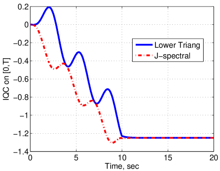
Figure 2: $\int_{0}^{T}\left(\Psi\left[\begin{smallmatrix}G\\ 1\end{smallmatrix}\right]u\right)^{T}M\left(\Psi\left[\begin{smallmatrix}G\\ 1\end{smallmatrix}\right]u\right)dt$ versus time $T$.

It can be shown that lower triangular factorizations have a $(2,2)$ entry that is non-minimum phase in general. Specifically, if $\Psi$ is lower triangular and $\Pi=\Psi^{\sim}J\Psi$ then the entries of $\Psi$ satisfy:

$$\Pi_{11} =\Psi_{11}^{\sim}\Psi_{11}-\Psi_{21}^{\sim}\Psi_{21}$$

$$\Pi_{12} =-\Psi_{21}^{\sim}\Psi_{22}$$

$$\Pi_{22} =-\Psi_{22}^{\sim}\Psi_{22}$$

These conditions imply that if $\Pi_{12}$ has poles in the left half plane then $\Psi_{22}$ must be non-minimum phase. Specifically, if $\Pi$ is a positive-negative multiplier then there exists $\epsilon>0$ such that $-\Pi_{22}(j\omega)\geq\epsilon I$ $\forall\omega\in R$. Hence it can be factorized as $-\Pi_{22}=H^{\sim}H$ where $H\in RH$ and $H^{-1}$ is anti-stable. In other words $H$ is stable and anti-minimum phase. This factorization can be constructed from the normal stable, minimum phase spectral factorization (Youla, 1961). Next, let $\{p_{i}\}_{i=1}^{N}$ denote the poles of $\Pi_{12}$ in the left half plane. Define $\Psi_{21}$ and $\Psi_{22}$ as

$$\Psi_{22}(s) :=H(s)\left(\prod_{i=1}^{N}\frac{s+\bar{p}_{i}}{s-p_{i}}\cdot I_{m}\right)$$ (25)

$$\Psi_{21}(s) :=\left(-\Pi_{12}(s)\Psi_{22}^{-1}(s)\right)^{\sim}$$ (26)

By construction, $\Psi_{22}$ is stable and anti-minimum phase. The inclusion of the Blaschke products in the definition of $\Psi_{22}$ does not impact the value of $\Psi_{22}^{\sim}\Psi_{22}$ on the imaginary axis. Thus $\Pi_{22}=\Psi_{22}^{\sim}\Psi_{22}$ on the imaginary axis by construction of $H$. This choice of $\Psi_{22}$ is required to ensure that $\Pi_{12}\Psi_{22}^{-1}$ is anti-stable and hence $\Psi_{21}$ is stable. Moreover, $\Psi_{21}^{\sim}\Psi_{22}=-\Pi_{12}$. A stable, stably invertible $\Psi_{11}$ can then be constructed from a spectral factorization of $\Pi_{11}+\Psi_{21}^{\sim}\Psi_{21}$. In this construction, any LHP poles of $\Pi_{12}$ appear as RHP zeros in $\Psi_{22}$.

6 Comparison between IQC and graph separation results

6.1 Stability results

In this section we develop two stability results for the feedback interconnection of two nonlinear systems. One of these results will be obtained using graph separation methods. For completeness, we state an IQC version of Corollary 5.1 in (Teel, 1996) as follows:

Theorem 3 (Teel (1996)).

Let $\Delta_{1}$ and $\Delta_{2}$ be two causal and bounded systems. Let $\Psi$ be a stable linear system. Assume that:

1. the feedback interconnection of $G$ and $\Delta$ is well-posed;

2. the time-domain IQC

   $$\int_{0}^{T}\left(\Psi\begin{bmatrix}u\\ \Delta_{1}u\end{bmatrix}\right)^{\top}M\left(\Psi\begin{bmatrix}u\\ \Delta_{1}u\end{bmatrix}\right)dt\geq 0,$$ (27)

   is satisfied for any $T>0$ and $u\in\mathcal{L}_{2e}[0,\infty)$;

3. the time-domain inverse-graph IQC

   $$\int_{0}^{T}\left(\Psi\begin{bmatrix}\Delta_{2}u\\ u\end{bmatrix}\right)^{\top}M\left(\Psi\begin{bmatrix}\Delta_{2}u\\ u\end{bmatrix}\right)dt<-\epsilon\left\|\begin{bmatrix}\Delta_{2}u\\ u\end{bmatrix}\right\|_{T}^{2},$$ (28)

   is satisfied for any $T>0$ and $u\in\mathcal{L}_{2e}[0,\infty)$.

Then the feedback interconnection between $\Delta_{1}$ and $\Delta_{2}$ is $\mathcal{L}_{2}$-stable.

In the spirit of Jönsson (2011), we can establish the following corollary for the interconnection of two nonlinear systems:

Corollary 1 (Corollary of Theorem 1).

Let $\Delta_{1}:\mathcal{L}^{l}_{2e}[0,\infty)\rightarrow\mathcal{L}^{m}_{2e}[0,\infty)$ and $\Delta_{2}:\mathcal{L}^{m}_{2e}[0,\infty)\rightarrow\mathcal{L}^{l}_{2e}[0,\infty)$ be bounded causal operators, and let $\Pi\in\mathbf{RL}_{\infty}^{(m+l)\times(m+l)}$. Assume that:

1. for every $\tau\in[0,1]$, the feedback interconnection of $\tau\Delta_{1}$ and $\tau\Delta_{2}$ is well-posed;

2. for every $\tau\in[0,1]$, $\tau\Delta_{1}$ satisfies the IQC defined by $\Pi$;

3. for every $\tau\in[0,1]$, $\tau\Delta_{2}$ strictly satisfies the inverse-graph IQC defined by $\Pi$.

Then, the feedback interconnection of $\Delta_{1}$ and $\Delta_{2}$ is stable.

Proof: The result follows from the application of the IQC theorem using

$$\Delta=\begin{bmatrix}\Delta_{1}&0\\ 0&\Delta_{2}\end{bmatrix}\text{ and }G=\begin{bmatrix}0&I\\ I&0\end{bmatrix},$$ (29)

and the following augmented multiplier:

$$\Pi_{a}=\begin{bmatrix}\Pi_{11}&0&\Pi_{12}&0\\ 0&-\Pi_{22}-\epsilon I&0&-\Pi_{12}^{*}\\ \Pi_{12}^{*}&0&\Pi_{22}&0\\ 0&-\Pi_{12}&0&-\Pi_{11}^{*}-\epsilon I\\ \end{bmatrix}$$ (30)

Some straightforward algebra is required to show that the conditions in Theorem 1 are satisfied.

Using Theorem 2, then it is possible to remove the homotopy condition in the above result if the matrix $\Pi$ is positive-negative. Formally we can state the following result:

Corollary 2 (Corollary of Theorem 3).

Let $\Delta_{1}:\mathcal{L}^{l}_{2e}[0,\infty)\rightarrow\mathcal{L}^{m}_{2e}[0,\infty)$ and $\Delta_{2}:\mathcal{L}^{m}_{2e}[0,\infty)\rightarrow\mathcal{L}^{l}_{2e}[0,\infty)$ be bounded causal operators, and let $\Pi\in\mathbf{RL}_{\infty}^{(m+l)\times(m+l)}$. Assume that:

1. the feedback interconnection of $\Delta_{1}$ and $\Delta_{2}$ is well-posed;

2. $\Delta_{1}$ satisfies the IQC defined by $\Pi$;

3. $\Delta_{2}$ strictly satisfies the inverse-graph IQC defined by $\Pi$;

4. $\Pi$ is a positive-negative multiplier.

Then, the feedback interconnection of $\Delta_{1}$ and $\Delta_{2}$ is stable.

Proof: If $\Pi$ is a positive-negative multiplier, then there exists a factorization $(\Psi,M)$ such that $\Psi$ and $\Psi^{-1}$ are both stable (Seiler, 2015). Therefore the factorization $(\Psi,M)$ is doubly-hard as it satisfies the conditions in Theorem 2. The frequency-domain conditions (ii) and (iii) can be transformed into truncated time-domain conditions by using the factorization $(\Psi,M)$. As a result, Theorem 3 can be used to establish the stability of feedback interconnection between $\Delta_{1}$ and $\Delta_{2}$.

Remark .

It would not be possible to prove Corollary 2 by using triangular factorizations as it fails to guarantee that condition (iii) is equivalent to the truncated time-domain condition (28).

6.2 Discussion

A naïve comparison of the results would suggest that condition (iv) in Corollary 2 an extra condition over the conditions of Corollary 1. It is well known that the homotopy condition in (II) is satisfied if $\Pi_{11}$ is positive. Similarly, the homotopy condition in (III) is satisfied if $\Pi_{22}$ is negative. Hence one can think of a superiority of Corollary 1 over Corollary 2.

However, if $\Delta_{1}$ and $\Delta_{2}$ are both nonlinear, the IQC theorem requires homotopy conditions for both systems. If condition (II) holds, the requirement of the condition to be true when $\tau=0$ implies $\Pi_{11}(j\omega)\geq 0$ for all $\omega\in\mathds{R}$. Similarly, if condition (III) holds, the same argument when $\tau=0$ implies $\Pi_{22}(j\omega)\leq-\epsilon I$ for some $\epsilon>0$.

A perturbation argument as in (Carrasco et al., 2012; Seiler, 2015) in conjunction with a substitution argument (Carrasco et al., 2013) is required here; although $\Pi_{11}(j\omega)\geq 0$ does not guarantee the existence of a factorization, the following Lemma ensures the existence of a new $\bar{\Pi}$ with $\bar{\Pi}_{11}(j\omega)\geq\delta I$ for some $\delta>0$, hence $\bar{\Pi}$ can be factorised:

Lemma 3.

Let $G\in\mathbf{RH}^{m\times l}_{\infty}$, let $\Delta:\mathcal{L}^{m}_{2e}[0,\infty)\rightarrow\mathcal{L}^{l}_{2e}[0,\infty)$ be a bounded causal operator. If conditions (2) and (3) in Theorem 1 are satisfied for some $\Pi$, then there exists some $\delta>0$ such that conditions (2) and (3) are satisfied for

$$\bar{\Pi}=\begin{bmatrix}\Pi_{11}+\delta I_{m}&\Pi_{12}\\ \Pi_{21}&\Pi_{22}\end{bmatrix}.$$

Proof: See Appendix.

Remark .

The counterpart result for Corollary 1 is trivially obtained as the only required condition that is the boundedness of $\Delta_{2}$.

As a result, we can consider without loss of generality that Corollary 1 can only be satisfied if $\Pi$ is positive-negative. In conclusion, the IQC theorem may only provide better results over the graph separation theory when (a) $\Delta_{2}$ is linear and (b) $\Pi_{22}$ is non-negative. Otherwise, graph separation and IQC theories lead to the same stability result for rational multipliers.

7 Conclusion

The aim of this paper is to complete the classification of IQC-factorizations. It concludes previous work presented in (Seiler, 2015; Carrasco and Seiler, 2015), establishing a novel connection between IQC and graph separation theories. Here we propose the term doubly-hard factorizations, where both frequency conditions can be transformed into truncated time-domain conditions. We show that the standard triangular factorization is hard factorization but fails to be a doubly-hard. Then it cannot be used to establish an equivalence between the IQC theorem and separation results in the truncated time-domain. We have shown that $(\Psi,M)$ is a doubly-hard factorization if $\Psi$ and $\Psi^{-1}$ are both stable.

The new results allow us to compare both theories for the feedback interconnection two nonlinear systems. As a result we conclude that the IQC theorem for two nonlinear system does not provide any significant advantage over its counterpart result derived using graph separation tools. However, the IQC theorem may provide some advantages when one of the system is linear and the term $\Pi_{22}$ is non-negative.

Appendix A Proof of Lemma 3

If condition (2) is satisfied for $\Pi$, then it is trivial that it is also satisfied for $\bar{\Pi}$ since

$$\begin{bmatrix}\widehat{u}(j\omega)\\ \widehat{\Delta u}(j\omega)\end{bmatrix}^{*}\begin{bmatrix}\delta I_{m}&0\\ 0&0\end{bmatrix}\begin{bmatrix}\widehat{u}(j\omega)\\ \widehat{\Delta u}(j\omega)\end{bmatrix}=\delta|\widehat{u}(j\omega)|^{2}\geq 0$$ (31)

for all $\omega\in\mathds{R}$. If condition (3) is satisfied for $\Pi$, then there exists $\epsilon>0$ such that

$$\begin{bmatrix}G(j\omega)\\ I\end{bmatrix}^{*}\Pi(j\omega)\begin{bmatrix}G(j\omega)\\ I\end{bmatrix}\leq-\epsilon I\qquad\forall\omega\in\mathds{R}.$$ (32)

Moreover, for any $\delta>0$, it follows

$$\begin{bmatrix}G(j\omega)\\ I\end{bmatrix}^{*}\begin{bmatrix}\delta I_{m}&0\\ 0&0\end{bmatrix}\begin{bmatrix}G(j\omega)\\ I\end{bmatrix}=\delta(G(j\omega)^{*}G(j\omega))\leq\delta\|G\|^{2}_{\infty}I,$$ (33)

for all $\omega$. As a result, taking $\delta=\frac{\epsilon}{2\|G\|^{2}_{\infty}}$,

$$\begin{bmatrix}G(j\omega)\\ I\end{bmatrix}^{*}\bar{\Pi}(j\omega)\begin{bmatrix}G(j\omega)\\ I\end{bmatrix}\leq-(\epsilon-\frac{\epsilon}{2})I=-\frac{\epsilon}{2}I\qquad\forall\omega\in\mathds{R},$$ (34)

Appendix B Proof of Lemma 2

For any $T\geq 0$, the frequency-domain inequality (20) can be converted into time-domain (by Parserval’s theorem) and re-arranged as

$$\int_{0}^{T}z(t)^{\top}Mz(t)dt\leq-\epsilon\int_{0}^{\infty}z(t)^{\top}z(t)dt-\int_{T}^{\infty}z(t)^{\top}Mz(t)dt$$ (35)

Note that $-\epsilon\int_{T}^{\infty}z(t)^{\top}z(t)dt\leq 0$ and hence the following bound is also valid:

$$\int_{0}^{T}z(t)^{\top}Mz(t)dt\leq-\epsilon\int_{0}^{T}z(t)^{\top}z(t)dt-\int_{T}^{\infty}z(t)^{\top}Mz(t)dt$$ (36)

Next let $\tilde{w}\in\mathcal{L}_{2}[0,\infty)$ be any signal satisfying $\tilde{w}_{T}=w_{T}$. Define $\tilde{v}=\Delta_{2}\tilde{w}$ and let $\tilde{z}=\Psi\left[\begin{smallmatrix}\tilde{v}\\ \tilde{w}\end{smallmatrix}\right]$ be the response of $\Psi$ with null initial condition. By causality of $\Delta_{2}$ and $\Psi$, $w_{T}=\tilde{w}_{T}$ implies $v_{T}=\tilde{v}_{T}$ and $z_{T}=\tilde{z}_{T}$. Hence for all $\tilde{w}$, it holds

$$\int_{0}^{T}z(t)^{\top}Mz(t)dt=\int_{0}^{T}\tilde{z}(t)^{\top}M\tilde{z}(t)dt.$$

Moreover, the IQC holds for any input/output pairs of $\Delta_{2}$. In particular, Equation 36 holds with $z$ replaced by $\tilde{z}$. As a result, any $\tilde{w}\in\mathcal{L}_{2}$ satisfying $\tilde{w}_{T}=w_{T}$ can be used to upper bound the integral $\int_{0}^{\infty}z(t)^{\top}Mz(t)dt$ obtained with $w$:

$$\int_{0}^{T}z(t)^{\top}Mz(t)dt\leq-\epsilon\int_{0}^{T}z(t)^{\top}z(t)dt-\int_{T}^{\infty}\tilde{z}(t)^{\top}M\tilde{z}(t)dt$$ (37)

Minimizing over all feasible $\tilde{w}$ yields the upper bound

$$\int_{0}^{T}z(t)^{\top}Mz(t)dt\leq-\epsilon\int_{0}^{T}z(t)^{\top}z(t)dt\\ +\inf_{\tilde{w}\in\mathcal{L}_{2},\tilde{w}_{T}=w_{T}}\left(-\int_{T}^{\infty}\tilde{z}(t)^{\top}M\tilde{z}(t)dt\right),$$ (38)

The suitable set of signals $\tilde{w}$ can be rewritten as

$$\tilde{w}(t)=\begin{cases}w(t)&\text{ if }t\leq T\\ w_{f}(t)&\text{ if }t>T\end{cases}$$

for any $w_{f}\in\mathcal{L}_{2}[T,\infty)$. We can rewrite the minimisation as

$$\int_{0}^{T}z(t)^{\top}Mz(t)dt\leq-\epsilon\int_{0}^{T}z(t)^{\top}z(t)dt+\\ \inf_{w_{f}\in\mathcal{L}_{2}[T,\infty)}\left(-\int_{T}^{\infty}\tilde{z}(t)^{\top}M\tilde{z}(t)dt\right),$$ (39)

such that $\tilde{v}=\Delta_{2}\tilde{w}$ and $\tilde{z}=\Psi\begin{bmatrix}\tilde{v}\\ \tilde{w}\end{bmatrix}$. The dependence on $\Delta_{2}$ can be removed following similar arguments to those given in  (Seiler, 2015). Partition $\tilde{v}=\Delta_{2}\tilde{w}$ as:

$$\tilde{v}(t)=\begin{cases}\Delta_{2}w(t)&\text{ if }t\leq T\\ v_{f}(t)&\text{ if }t>T\end{cases}$$ (40)

The bound in Equation 39 only involves $\tilde{z}$ defined on $[T,\infty)$. This signal can be computed from the state of $\Psi$ at time $T$, i.e. $x_{T}$, as well as the signals $w_{f}$ and $v_{f}$. Note that $x(T)=x_{T}$ is the same for any feasible choice of $\tilde{w}$ because $\tilde{w}_{T}=w_{T}$ and $\tilde{v}_{T}=v_{T}$. The dependence on $\Delta_{2}$ is removed, with some conservatism, by simply maximizing over all possible future signals $v_{f}$ defined on $[T,\infty)$ instead of using $\tilde{v}=\Delta_{2}w$. In other words,

$$\int_{0}^{T}z(t)^{\top}Mz(t)dt\leq-\epsilon\int_{0}^{T}z(t)^{\top}z(t)dt+\\ \inf_{w_{f}\in\mathcal{L}_{2}[T,\infty)}\sup_{v_{f}\in\mathcal{L}_{2}[T,\infty)}\left(-\int_{T}^{\infty}\tilde{z}(t)^{\top}M\tilde{z}(t)dt\right),$$ (41)

This is subject to constraint $x(T)=x_{T}$. This can be rewritten using the cost function $J$ as:

$$\int_{0}^{T}z(t)^{\top}Mz(t)dt\leq-\epsilon\int_{0}^{T}z(t)^{\top}z(t)dt-\underline{J}(x_{T}),$$ (42)

References

- Carrasco and Seiler (2015) J. Carrasco and P. Seiler. Integral quadratic constraint theorem: A topological separation approach. In 2015 54th IEEE Conference on Decision and Control (CDC), pages 5701–5706, 2015.
- Carrasco et al. (2012) J. Carrasco, W. P. Heath, and A. Lanzon. Factorization of multipliers in passivity and IQC analysis. Automatica, 48(5):609–616, 2012.
- Carrasco et al. (2013) J. Carrasco, W. P. Heath, and A. Lanzon. Equivalence between classes of multipliers for slope-restricted nonlinearities. Automatica, 49(6):1732 – 1740, 2013.
- Desoer and Vidyasagar (1975) C. A. Desoer and M. Vidyasagar. Feedback Systems: Input-Output Properties. Academic Press, Inc., Orlando, FL, USA, 1975.
- Georgiou and Smith (1997) T.T. Georgiou and M.C. Smith. Robustness analysis of nonlinear feedback systems: an input-output approach. Automatic Control, IEEE Transactions on, 42(9):1200–1221, 1997.
- Goh (1996) K.-C. Goh. Structure and factorization of quadratic constraints for robustness analysis. In Decision and Control, 1996., Proceedings of the 35th IEEE, volume 4, pages 4649 –4654, 1996.
- Goh and Safonov (1995) K.-C. Goh and M.G. Safonov. Robust analysis, sectors, and quadratic functionals. In Decision and Control, 1995., Proceedings of the 34th IEEE Conference on, volume 2, pages 1988 –1993, 1995.
- Isidori (2013) A. Isidori. Nonlinear control systems. Springer Science & Business Media, 2013.
- Jönsson (1996) U. T. Jönsson. Robustness Analysis of Uncertain and Nonlinear Systems. PhD thesis, Department of Automatic Control, Lund Institute of Technology, 1996.
- Jönsson (2011) U.T. Jönsson. Stability of systems interconnected over circular graphs. In IFAC 2011 World Congress, pages 3378–3383, 2011.
- Megretski (2010) A. Megretski. KYP lemma for non-strict inequalities and the associated minimax theorem. arXiv, page 1008.2552, 2010.
- Megretski and Rantzer (1997) A. Megretski and A. Rantzer. System analysis via integral quadratic constraints. Automatic Control, IEEE Transactions on, 42(6):819 –830, 1997.
- Partington (2004) J.R. Partington. Linear Operators and Linear Systems: An Analytical Approach to Control Theory. London Mathematical Society Student Texts. Cambridge University Press, 2004.
- Safonov (1980) M. Safonov. Stability and robustness of multipvariable feedback systems. The MIT Press, 1980.
- Scherer and Weiland (2000) C. Scherer and S. Weiland. Linear matrix inequalities in control. Lecture Notes, Dutch Institute for Systems and Control, Delft, The Netherlands, 2000.
- Seiler (2015) P. Seiler. Stability analysis with dissipation inequalities and integral quadratic constraints. IEEE Transactions on Automatic Control, 60(6):1704 – 1709, 2015.
- Seiler et al. (2010) P. Seiler, A. Packard, and G.J. Balas. A dissipation inequality formulation for stability analysis with integral quadratic constraints. In Decision and Control (CDC), 2010 49th IEEE Conference on, pages 2304 –2309, 2010.
- Teel (1996) A.R. Teel. On graphs, conic relations, and input-output stability of nonlinear feedback systems. Automatic Control, IEEE Transactions on, 41(5):702 –709, 1996.
- Veenman and Scherer (2013) J. Veenman and C.W. Scherer. Stability analysis with integral quadratic constraints: A dissipativity based proof. In Decision and Control (CDC), 2013 IEEE 52nd Annual Conference on, pages 3770–3775, 2013.
- Yakubovich (1965) V. A. Yakubovich. Frequency conditions for the absolute stability and dissipativity of control systems with a single differentable nonlinearity. Soviet Mathematics Doklady, 6:98–101, 1965.
- Yakubovich (1967) V. A. Yakubovich. Frequency conditions for the absolute stability of control systems with several nonlinear or linear nonstationary blocks. Automation and Remote Control, 28:857–880, 1967.
- Yakubovich (1971) V. A. Yakubovich. S-procedure in nonlinear control theory. Vestnik Leningrad University, 1:62–77, 1971.
- Youla (1961) D. Youla. On the factorization of rational matrices. IRE Transactions on Information Theory, 7(3):172–189, 1961.
- Zames and Falb (1968) G. Zames and P. L. Falb. Stability conditions for systems with monotone and slope-restricted nonlinearities. SIAM Journal on Control, 6(1):89–108, 1968.