$k$-means as a variational EM approximation of Gaussian mixture models

Abstract

We show that $k$-means (Lloyd’s algorithm) is obtained as a special case when truncated variational EM approximations are applied to Gaussian Mixture Models (GMM) with isotropic Gaussians. In contrast to the standard way to relate $k$-means and GMMs, the provided derivation shows that it is not required to consider Gaussians with small variances or the limit case of zero variances. There are a number of consequences that directly follow from our approach: (A) $k$-means can be shown to increase a free energy associated with truncated distributions and this free energy can directly be reformulated in terms of the $k$-means objective; (B) $k$-means generalizations can directly be derived by considering the 2nd closest, 3rd closest etc. cluster in addition to just the closest one; and (C) the embedding of $k$-means into a free energy framework allows for theoretical interpretations of other $k$-means generalizations in the literature. In general, truncated variational EM provides a natural and rigorous quantitative link between $k$-means-like clustering and GMM clustering algorithms which may be very relevant for future theoretical and empirical studies.

1 Introduction

Clustering is the task of associating a set of $N$ data points with a set of $C$ clusters (typically with $C\ll{}N$), where such an association is defined by a high similarity of points within one cluster compared to the similarity of any two points of different clusters. Different criteria for data point similarity and different algorithmic properties have led to the development of a large variety of clustering algorithms in the course of more than half a century. Two of the presumably most influential classes of algorithms are $k$-means-like algorithms (Lloyd, 1982; Jain, 2010, and many more) and Gaussian Mixture Models (GMMs).

$k$-means. The $k$-means algorithm and its many variants (e.g. Steinley, 2006) have been used since the 1950’s and are often considered as the most popular clustering algorithms (Berkhin, 2006). If we denote by $\vec{y}^{\,(1:N)}=\vec{y}^{\,(1)},\ldots,\vec{y}^{\,(N)}$ the data points (with $\vec{y}^{\,(n)}\in\mathbbm{R}^{D}$) and by $\vec{\mu}_{1:C}=\vec{\mu}_{1},\ldots,\vec{\mu}_{C}$ the cluster centers (with $\vec{\mu}_{c}\in\mathbbm{R}^{D}$), then the most common form of $k$-means is given by Alg. 1, with $\|\cdot\|$ as Euclidean metric. After initialization of $\vec{\mu}_{1:C}$, Alg. 1 increases the $k$-means objective given by

$${\cal J}(s^{(1:N)}_{1:C},\vec{\mu}_{1:C})=\displaystyle\sum_{n=1}^{N}\sum_{c=1}^{C}s_{c}^{(n)}\,\|\vec{y}^{\,(n)}\,-\,\vec{\mu}_{c}\|^{2}\,.$$ (1)

The updates of $s_{c}^{(n)}$ and $\vec{\mu}_{c}$ in Alg. 1 are usually derived from (1). Because of its few elementary algorithmic steps, $k$-means is easy to implement, and it has been observed to work very well in practice (e.g. Duda et al., 2001).

repeat

       for $c=1,\ldots,C$ and $n=1,\ldots,N$ do

             $s_{c}^{(n)}=\left\{\begin{array}[]{cl}1&\mbox{if }\forall{}c^{\prime}\neq{}c:\|\vec{y}^{\,(n)}-\vec{\mu}_{c}\|<\|\vec{y}^{\,(n)}-\vec{\mu}_{c^{\prime}}\|\\[2.84526pt] 0&\mbox{otherwise;}\end{array}\right.$

      for $c=1,\ldots,C$ do

             $\vec{\mu}_{c}=\sum_{n=1}^{N}s_{c}^{(n)}\,\vec{y}^{\,(n)}/\sum_{n=1}^{N}s_{c}^{(n)}$;

      

until $\vec{\mu}_{1:C}$ have converged;

Algorithm 1 $k$-means.

GMM. GMM-based clustering algorithms (e.g. McLachlan and Basford, 1988) are derived from a probabilistic data model $p(\vec{y}\,|\,\Theta)$. While general GMMs allow for different mixing proportions and multivariate Gaussian distributions, we will for the purposes of this study consider equal mixing proportions and equally sized, isotropic Gaussians:

$${}p(c\,|\,\Theta) =\frac{1}{C}\,,\ \ \displaystyle p(\vec{y}\,|\,c,\Theta)=\textstyle(2\pi\sigma^{2})^{-\frac{D}{2}}\exp\!\big{(}-\frac{1}{2\sigma^{2}}\|{}\vec{y}-\vec{\mu}_{c}\|{}^{2}\big{)},$$ (2)

i.e., we will use a ‘flat’ prior $p(c\,|\,\Theta)$ and equal and isotropic variance $\sigma^{2}$ of the clusters. The most standard form to update the GMM model parameters $\Theta=(\vec{\mu}_{1:C},\sigma^{2})$ is derived using expectation maximization (EM; Dempster et al., 1977), which results for GMM (2) in Alg.  2 (Barber, 2012, & refs. therein).

repeat

       for $c=1,\ldots,C$ and $n=1,\ldots,N$ do

             $r_{c}^{(n)}=\frac{\textstyle\exp\!\big{(}-\frac{1}{2\sigma^{2}}\|{}\vec{y}^{\,(n)}-\vec{\mu}_{c}\|{}^{2}\big{)}}{\textstyle\sum_{c^{\prime}=1}^{C}\exp\!\big{(}-\frac{1}{2\sigma^{2}}\|{}\vec{y}^{\,(n)}-\vec{\mu}_{c^{\prime}}\|{}^{2}\big{)}};\phantom{iiii}\mbox{}$

      for $c=1,\ldots,C$ do

             $\begin{array}[]{lll}\vec{\mu}_{c}&=\sum_{n=1}^{N}r_{c}^{(n)}\vec{y}^{\,(n)}/\sum_{n=1}^{N}r_{c}^{(n)};&\mbox{}\vspace{1.5mm}\\ \end{array}$

      $\begin{array}[]{lll}\sigma^{2}&=\frac{1}{DN}\,\!\!\sum_{n,\,c=1}^{N,C}r_{c}^{(n)}\,\|\vec{y}^{\,(n)}-\vec{\mu}_{c}\|^{2};&\mbox{}\vspace{1.5mm}\\ \end{array}$

until parameters $\Theta$ have converged;

Algorithm 2 EM for GMM.

After initialization of $\Theta=(\vec{\mu}_{1:C},\sigma^{2})$, the algorithm maximizes the data log-likelihood given by:

$${\cal L}(\Theta)=\frac{1}{N}\sum_{n=1}^{N}\log\!\Big{(}\sum_{c=1}^{C}\frac{1}{C}\,{\cal N}\big{(}\vec{y}^{\,(n)};\vec{\mu}_{c},\sigma^{2}\hbox{$1\hskip-1.2pt\vrule depth=0.0pt,height=6.88889pt,width=0.7pt\vrule depth=0.0pt,height=0.3pt,width=1.19995pt$}\big{)}\Big{)}\,,$$ (3)

with ${\cal N}(\vec{y}^{\,(n)};\vec{\mu}_{c},\sigma^{2}\hbox{$1\hskip-1.2pt\vrule depth=0.0pt,height=6.88889pt,width=0.7pt\vrule depth=0.0pt,height=0.3pt,width=1.19995pt$})$ as given in (2). Note that (3) is normalized by the number of data points for this study. As is customary for GMMs, we refer to the posteriors $p(c\,|\,\vec{y}^{\,(n)},\Theta)$ as responsibilities (abbreviate by $r_{c}^{(n)}$). Computing the $r_{c}^{(n)}$ in Alg. 2 is referred to as E-step, while updates of parameters $\vec{\mu}_{1:C}$ and $\sigma^{2}$ in Alg. 2 are referred to as M-step.
Related Work and Our Contribution. The popularity of $k$-means and GMM algorithms has resulted in many theoretical as well as empirical studies of their functional and theoretical properties. Considerable progress using novel versions could be made, and much insight could be gained for $k$-means (Har-Peled and Sadri, 2005; Arthur and Vassilvitskii, 2006; Arthur et al., 2009; Bachem et al., 2016) and GMMs (Chaudhuri et al., 2009; Kalai et al., 2010; Moitra and Valiant, 2010; Belkin and Sinha, 2010; Xu et al., 2016) relatively recently. Because of their similarity, $k$-means and GMMs have long been formally related to each other. It is thus well-known (see, e.g. MacKay, 2003; Barber, 2012, & refs. therein) that $k$-means (Alg. 1) can be obtained as a limit case of EM for GMM (2). This limit is given by considering increasingly small $\sigma^{2}$, i.e., $\sigma^{2}\rightarrow{}0$. The responsibilities $r_{c}^{(n)}$ in Alg. 2 then become equal to one for the closest cluster and zero otherwise, and the $k$-means algorithm (Alg. 1) is recovered. Furthermore, approaches using algorithms which modify EM algorithms by introducing additional ‘hard’ assignment steps of data points to clusters have been used to relate $k$-means and GMM clustering. Given a generative model, such approaches are often referred to as ‘hard’ EM (e.g. Segal et al., 2002; Van den Oord and Schrauwen, 2014), as ‘classification EM’ (CEM; e.g. Celeux and Govaert, 1992) for GMMs, or as ‘Viterbi training’ for HMMs (e.g. Allahverdyan and Galstyan, 2011). For data distributions with negligible cluster overlap (a setting which is closely related to the limit $\sigma^{2}\rightarrow{}0$), ‘hard’ assignment algorithms can be shown to be equivalent to standard EM (e.g. Celeux and Govaert, 1992). ‘Hard’ assignments can also be informally interpreted as a variational approach but (to the knowledge of the authors) neither proofs nor quantitative results have been provided (compare Suppl. B). In contrast to ‘hard’ cluster assignments, the assignment is ‘soft’ in EM for GMMs. ‘Hard’ assignments have sometimes been considered disadvantageous as the relative importance of the clusters for the data points is not taken into account. Different $k$-means generalizations have therefore been suggested, e.g., with aims to enhance $k$-means convergence Har-Peled and Sadri (2005) or to relax its ‘hard’ cluster assignment (e.g. Bezdek, 1981; Celeux and Govaert, 1992; MacKay, 2003; Miyamoto et al., 2008). As for clustering in general, $k$-means also remained of interest in the probabilistic Machine Learning community, and notably in the field of non-parametric approaches. Welling and Kurihara (2006) suggested ‘Bayesian $k$-means’, for instance, and used variational Bayesian approximations in order to obtain $k$-means-like run time behavior for model selection. Later on, Kulis and Jordan (2012) also used a Bayesian treatment, and combined it with the relation of $k$-means to GMMs obtained in the limit $\sigma^{2}\rightarrow{}0$. In this way they derived new ‘hard assignment’ algorithms based on a Gibbs sampler used within a non-parametric approach (also compare Broderick et al., 2013).

In this work, we derive the $k$-means algorithm from a novel class of variational EM algorithms applied to GMMs. Most notably $k$-means is obtained cleanly and rigorously without any assumptions on $\sigma^{2}$. Variational EM seeks to optimize a lower bound (the free energy; Neal and Hinton,1998) of the data log-likelihood by making use of variational distributions that approximate full posterior probabilities. The free energy is also frequently referred to as the evidence lower bound (ELBO; e.g. Hoffman et al., 2013). For our study, we apply truncated posteriors (Lücke and Eggert, 2010) as variational distributions in their fully variational formulation (Lücke, 2018). After having shown that $k$-means is a variational approximation, $k$-means and its generalizations can be quantitatively related to GMMs without taking the limit to zero cluster variances or without assuming $\sigma$ to be small compared to cluster-to-cluster distances. Furthermore, the observation that $k$-means is a variational optimization implies that it optimizes a lower bound of a GMM log-likelihood. Hence, we can derive lower free energy bounds for $k$-means and its generalizations that quantify the link between the $k$-means and the GMM objective. As such we provide a closer theoretical link between these two central classes of clustering methods than has previously been established.

Truncated approaches have been applied to mixture models before. Work by Dai and Lücke (2014) used truncated approximations for a position invariant mixture model, and Forster et al. (2018) for a hierarchical Poisson mixture. Work by Shelton et al. (2014) was the first to apply truncated EM to standard GMMs, followed by Hughes and Sudderth (2016) who additionally used a constraint likelihood optimization to find cluster centers for truncated posteriors. None of these contributions has derived $k$-means as a variational EM algorithm for GMMs nor did any contribution provide quantitative free energy results or the links to generalizations of $k$-means derived in this study.

2 Truncated variational EM and GMMs

The basic idea of truncated EM is the use of truncated approximations of exact posterior distributions (e.g. Lücke and Eggert, 2010; Sheikh et al., 2014). In the notation as used for GMMs above, the truncated approximation takes the form:

$$r_{c}^{(n)}\approx q_{c}^{(n)}=\frac{p(c,\vec{y}^{\,(n)}\,|\,\Theta)}{\textstyle\sum_{c^{\prime}\in\,{\cal K}^{(n)}}p(c^{\prime},\vec{y}^{\,(n)}\,|\,\Theta)}\,\delta(c\in{\cal K}^{(n)})\,,$$ (4)

where ${\cal K}^{(n)}$ is a set of cluster indices (containing different clusters $c$ associated with data point $\vec{y}^{\,(n)}$). Suppl. A and Fig. S1 provide an example. The set of all ${\cal K}^{(n)}$ we denote by ${\cal K}$, i.e., ${\cal K}=({\cal K}^{(1:N)})$. As is customary for truncated distributions (Lücke and Eggert, 2010; Dai and Lücke, 2014; Shelton et al., 2014; Hughes and Sudderth, 2016), we take the sizes of all ${\cal K}^{(n)}$ to be equal, $|{\cal K}^{(n)}|=C^{\prime}$, with $1\leq C^{\prime}\leq C$. The truncated approximation (4) is a good approximation if ${\cal K}^{(n)}$ contains all those clusters with significant posterior mass $p(c\,|\,\vec{y}^{\,(n)},\Theta)$ (i.e., significant non-zero responsibilities $r_{c}^{(n)}$). Truncated approaches can represent very accurate approximations for many data sets, as typically most responsibilities are negligible.

In order to derive a learning algorithm for GMMs based on truncated distributions, we have to answer the question how the parameters ${\cal K}^{(n)}$ and $\Theta$ are to be updated. For our purposes we will here make use of a recent study which addressed this question for general models (with discrete latents) by embedding truncated distributions into a fully variational optimization framework (Lücke, 2018). More specifically, we use the result of Lücke (2018) that the free energy as a lower bound of the data likelihood is monotonically increased if: (A) the parameters $\Theta$ are updated using standard M-steps, with exact posteriors replaced by truncated posteriors; and (B) that the sets ${\cal K}^{(n)}$ can be found using a simplified expression for the free energy.

For GMMs, this means that we can use the standard M-steps of Alg. 2 and replace $r_{c}^{(n)}$ with the truncated approximations $q_{c}^{(n)}$ in (4). For the GMM (2), the truncated responsibilities and M-steps are thus:

$$q_{c}^{(n)} =\frac{\textstyle\exp\!\big{(}-\frac{1}{2\sigma^{2}}\|{}\vec{y}^{\,(n)}-\vec{\mu}_{c}\|{}^{2}\big{)}}{\textstyle\sum_{c^{\prime}\in{\cal K}^{(n)}}\exp\!\big{(}-\frac{1}{2\sigma^{2}}\|{}\vec{y}^{\,(n)}-\vec{\mu}_{c^{\prime}}\|{}^{2}\big{)}}\,\delta(c\in{\cal K}^{(n)})$$ (5)

$$\vec{\mu}^{\mathrm{\,new}}_{c} =\frac{\sum_{n=1}^{N}{}q_{c}^{(n)}\vec{y}^{\,(n)}}{\sum_{n=1}^{N}{}q_{c}^{(n)}},\,\,\,\,\,\sigma_{\mathrm{new}}^{2}=\frac{1}{DN}\!\!\sum_{n,c=1}^{N,C}q_{c}^{(n)}\,\|\vec{y}^{\,(n)}-\vec{\mu}^{\mathrm{\,new}}_{c}\|^{2}$$ (6)

The parameters ${\cal K}^{(n)}$ of the truncated distributions $q_{c}^{(n)}$ have to be found in the variational E-step. In order to do so, we use the simplified free energy derived in (Lücke, 2018, Prop. 3), which takes for our GMM (2) the following form:

$${\cal F}({\cal K},\Theta) =\textstyle\frac{1}{N}\sum_{n=1}^{N}\log\!\Big{(}\!\sum_{c\in{\cal K}^{(n)}}p(c,\vec{y}^{\,(n)}\,|\,\Theta)\Big{)}$$

$$=\textstyle\frac{1}{N}\sum_{n=1}^{N}\log\!\Big{(}\!\sum_{c\in{\cal K}^{(n)}}\frac{1}{C}\,{\cal N}\big{(}\vec{y}^{\,(n)};\,\vec{\mu}_{c},\sigma^{2}\hbox{$1\hskip-1.2pt\vrule depth=0.0pt,height=6.88889pt,width=0.7pt\vrule depth=0.0pt,height=0.3pt,width=1.19995pt$}\big{)}\Big{)}.$$ (7)

The truncated variational E-step (TV-E-step) first optimizes ${\cal F}({\cal K},\Theta)$ w.r.t. ${\cal K}$ and the obtained truncated responsibilities $q_{c}^{(n)}$ are then used in the M-step (6) to optimize ${\cal F}({\cal K},\Theta)$ w.r.t. $\Theta$. The form of the free energy (7) and the result that it is monotonically increased by iterating TV-E-step and M-step are the crucial theoretical results by Lücke (2018) that are used in this study. Neither of these two results is straight-forward: (A) truncated distributions themselves depend on the model parameters $\Theta$, and (B) it requires a number of derivations exploiting specific properties of truncated distributions to obtain the concise form used for expression (7).

The TV-E-step now requires finding sets ${\cal K}^{(n)}$ which increase ${\cal F}({\cal K},\Theta)$. The free energy (7) is computationally tractable, so a new ${\cal K}$ could in principle be found by directly comparing ${\cal F}({\cal K}^{\mathrm{new}},\Theta)$ of a new ${\cal K}^{\mathrm{new}}$ with ${\cal F}({\cal K}^{\mathrm{old}},\Theta)$ of the current ${\cal K}^{\mathrm{old}}$. We can slightly reformulate the problem by considering a specific data point $n$ and cluster $\tilde{c}\in{\cal K}^{(n)}$ for which we ask when any other replacing cluster $c\not\in{\cal K}^{(n)}$ would increase the free energy ${\cal F}({\cal K},\Theta)$. By virtue of the properties of GMM (2) and due to the specific structure of the free energy (summation and concavity of the logarithm in Eqn. 7), we can then show:
 
Proposition 1
Consider the GMM (2) and the free energy (7) for $n=1:N$ data points $\vec{y}^{\,(n)}\in\mathbbm{R}^{D}$. Furthermore, consider for a fixed $n$ the replacement of a cluster $\tilde{c}\in{\cal K}^{(n)}$ by a cluster $c\not\in{\cal K}^{(n)}$. Then the free energy ${\cal F}({\cal K},\Theta)$ increases if and only if

$$\|\vec{y}^{\,(n)}\,-\,\vec{\mu}_{c}\|<\|\vec{y}^{\,(n)}\,-\,\vec{\mu}_{\tilde{c}}\|\,.$$ (8)

Proof
First observe that the free energy is increased if $p(c,\vec{y}^{\,(n)}\,|\,\Theta)>p(\tilde{c},\vec{y}^{\,(n)}\,|\,\Theta)$ because of the summation over $c$ in (7) and because of the concavity of the logarithm. Analogously, the free energy stays constant or decreases for $p(c,\vec{y}^{\,(n)}\,|\,\Theta)\leq{}p(\tilde{c},\vec{y}^{\,(n)}\,|\,\Theta)$. If we use the GMM (2), we obtain for the joint:

$$\textstyle p(c,\vec{y}\,|\,\Theta)=\frac{1}{C}(2\pi\sigma^{2})^{-\frac{D}{2}}\exp\!\big{(}-\frac{1}{2\sigma^{2}}\|{}\vec{y}-\vec{\mu}_{c}\|{}^{2}\big{)}.$$ (9)

The first two factors are independent of the data point and cluster. The criterion for an increase of the free energy can therefore be reformulated as follows:

$$p(c,\vec{y}\,|\,\Theta) >p(\tilde{c},\vec{y}\,|\,\Theta)$$

$$\Leftrightarrow{} \textstyle\exp\!\big{(}-\frac{1}{2\sigma^{2}}\|\vec{y}-\vec{\mu}_{c}\|^{2}\big{)} \textstyle>\exp\!\big{(}-\frac{1}{2\sigma^{2}}\|\vec{y}-\vec{\mu}_{\tilde{c}}\|^{2}\big{)}$$

$$\Leftrightarrow{} \textstyle\|\vec{y}-\vec{\mu}_{c}\| <\|\vec{y}-\vec{\mu}_{\tilde{c}}\|\,.\vspace{-4mm}$$

$\square$
Prop. 1 means that we have to replace clusters in ${\cal K}^{(n)}$ that are relatively distant from $\vec{y}^{\,(n)}$ by those closer to $\vec{y}^{\,(n)}$ in order to increases the free energy ${\cal F}({\cal K},\Theta)$. Any such procedure gives with M-step (6) rise to a variational EM algorithm that monotonically increases the lower bound (7) of likelihood (3). For an arbitrary generative model, the degree how much ${\cal F}({\cal K},\Theta)$ is increased or how long one should seek new clusters in the E-step is a design choice of the algorithm. In the case of GMMs (and other mixture models) we can exhaustively enumerate all clusters such that ${\cal F}({\cal K},\Theta)$ can be fully maximized.
Corollary 1
Same prerequisites as for Prop. 1. The free energy ${\cal F}({\cal K},\Theta)$ is maximized w.r.t. ${\cal K}$ (with fixed $\Theta$) if and only if for all $n$ the set ${\cal K}^{(n)}$ contains the $C^{\prime}$ clusters closest to data point $\vec{y}^{\,(n)}$.
Proof
We assume that there are no equal distances among all pairs of data points and cluster centers. If ${\cal K}^{(n)}$ contains the $C^{\prime}$ closest clusters, it applies: $\forall{}c\in{\cal K}^{(n)},\ \forall{}\tilde{c}\not\in{\cal K}^{(n)}:\|{}\vec{y}^{\,(n)}\,-\,\vec{\mu}_{c}\|{}<\|{}\vec{y}^{\,(n)}\,-\,\vec{\mu}_{\tilde{c}}\|{}$. If we now consider an arbitrary $n$ and replace an arbitrary $c\in{\cal K}^{(n)}$ by an arbitrary $c^{\mathrm{new}}\not\in{\cal K}^{(n)}$ it applies $\|{}\vec{y}^{\,(n)}\,-\,\vec{\mu}_{c^{\mathrm{new}}}\|{}>\|{}\vec{y}^{\,(n)}\,-\,\vec{\mu}_{c}\|{}$ such that by virtue of Prop. 1 ${\cal F}({\cal K},\Theta)$ decreases. As any arbitrary such replacement (any change of ${\cal K}$) results in a decrease of the free energy, ${\cal F}({\cal K},\Theta)$ is maximized if ${\cal K}$ contains the $C^{\prime}$ closest clusters.
$\square$
We can now formulate a truncated variational EM (TV-EM) algorithm for GMM (2), here referred to as $k$-means-$C^{\prime}$ (Alg. 3).

set $|{\cal K}^{(n)}|=C^{\prime}$ for all $n$ and init $\vec{\mu}_{1:C}$ and $\sigma^{2}$;

repeat

       for $n=1,\ldots,N$ do

             define ${\cal K}^{(n)}$ such that $\forall{}c\in{\cal K}^{(n)}\ \forall{}\tilde{c}\not\in{\cal K}^{(n)}$:

             $\|{}\vec{y}^{\,(n)}\,-\,\vec{\mu}_{c}\|{}<\|{}\vec{y}^{\,(n)}\,-\,\vec{\mu}_{\tilde{c}}\|{}$;

      compute $q_{c}^{(n)}$ for all $c$ and $n$ using (5);

       update $\vec{\mu}_{1:C}$ and $\sigma^{2}$ using (6);

until $\vec{\mu}_{1:C}$ and $\sigma^{2}$ have converged;

Algorithm 3 The $k$-means-$C^{\prime}$ algorithm.

3 $k$-means and truncated variational EM for GMMs

TV-EM for GMMs (Alg. 3) increases the similarity between $k$-means and standard EM for GMMs in two ways: (A) it relates Euclidean distances to a variational free energy and thus to the GMM likelihood; and (B) it introduces ‘hard’ zeros in the updates of model parameters (some or many $q_{c}^{(n)}$ are zero). Crucial remaining differences are, however, (A) the weighted updates of the cluster centers in Eqn. 6 compared to the $k$-means update, and (B) the update of the cluster variance $\sigma^{2}$ in Eqn. 6 along with the cluster centers for Alg. 3 which does not have a correspondence in $k$-means. By considering the first difference, the obvious next step is to consider a boundary case of Alg. 3 by demanding that the sets ${\cal K}^{(n)}$ shall contain just one element, i.e., we set $C^{\prime}=1$. All derivations above apply for all $1\leq{}C^{\prime}\leq{}C$, and while standard EM for the GMM (2) is recovered for $C^{\prime}=C$, we find that for $C^{\prime}=1$ standard $k$-means (Alg. 1) is recovered.
Proposition 2
Consider the TV-EM algorithm (Alg. 3) for the GMM (2) with $\sigma^{2}>0$. If we set $C^{\prime}=1$, then the TV-EM updates of the cluster centers $\vec{\mu}_{c}$ (6) become independent of the variance $\sigma^{2}$ and are given by the standard $k$-means algorithm in Alg. 1.
Proof
If we choose $|{\cal K}^{(n)}|=C^{\prime}=1$ for all $n$, then each ${\cal K}^{(n)}$ computed in the TV-E-step of Alg. 3 contains according to Corollary 1 the index of the cluster center closest to $\vec{y}^{\,(n)}$ as only element. If we denote these centers by $c_{o}^{(n)}$, we get ${\cal K}^{(n)}=\{c_{o}^{(n)}\}$ and obtain for the truncated responsibilities $q_{c}^{(n)}$ in (5):

$$q_{c}^{(n)} =\frac{\textstyle\exp\!\big{(}\!-\!\frac{1}{2\sigma^{2}}\|{}\vec{y}-\vec{\mu}_{c}\|{}^{2}\big{)}\,\delta(c=c_{o}^{(n)})}{\textstyle\sum_{c^{\prime}\in\{c_{o}^{(n)}\}}\exp\!\big{(}\!-\!\frac{1}{2\sigma^{2}}\|{}\vec{y}-\vec{\mu}_{c^{\prime}}\|{}^{2}\big{)}}=\left\{\begin{array}[]{@{\hspace{2pt}}l@{\hspace{7pt}}l@{\hspace{-2pt}}}\hskip 2.0pt\lx@intercol 1\hfil\hskip 7.0&\mbox{if\ \ }c=c_{o}^{(n)}\\ \hskip 2.0pt\lx@intercol 0\hfil\hskip 7.0&\mbox{otherwise}\end{array}\right.,$$ (12)

which is identical to $s_{c}^{(n)}$ in Alg. 1. By using $q_{c}^{(n)}=s_{c}^{(n)}$ for the M-step, we consequently obtain:

$$\phantom{i}\vec{\mu}^{\mathrm{\,new}}_{c}\!=\frac{\textstyle\sum_{n=1}^{N}{}s_{c}^{(n)}\vec{y}^{\,(n)}}{\textstyle\sum_{n=1}^{N}{}s_{c}^{(n)}},\,\,\,\sigma_{\mathrm{new}}^{2}=\frac{1}{DN}\!\sum_{n,c=1}^{N,C}\!s_{c}^{(n)}\,\|\vec{y}^{\,(n)}-\vec{\mu}^{\mathrm{\,new}}_{c}\|^{2}.\$$ (13)

Now observe that the computation of $q_{c}^{(n)}=s_{c}^{(n)}$ and the updates of the $\vec{\mu}_{c}$ do not involve the parameter $\sigma^{2}$. The cluster centers $\vec{\mu}_{c}$ can thus be optimized without requiring knowledge about the cluster variances $\sigma^{2}$, i.e., the $\vec{\mu}_{c}$ optimization becomes independent of $\sigma^{2}$. As the TV-EM updates for $q_{c}^{(n)}$ and $\vec{\mu}_{c}$ are identical to the updates of $s_{c}^{(n)}$ and $\vec{\mu}_{c}$ in Alg. 1, the optimization procedure for the $\vec{\mu}_{c}$ is given by the standard $k$-means algorithm.
$\square$
A direct consequence of Prop. 2 is that standard $k$-means provably monotonically increases the truncated free energy (7) with $C^{\prime}=1$. Notably, only for this choice of $C^{\prime}$ the updates of cluster means and variance decouple. We can, of course, add the variance updates to standard $k$-means but this does not effect the $\vec{\mu}_{c}$ updates. With or without $\sigma^{2}$ updates the free energy monotonically increases. If our goal is the maximization of the free energy objective, the $\sigma^{2}$ updates should be included, however. According to the independence of $\vec{\mu}_{c}$-optimization from $\sigma^{2}$, it would be sufficient to update $\sigma^{2}$ once and only after $k$-means has optimized the cluster centers.

Prop. 2 shows that $k$-means is obtained from a variational free energy objective. This free energy is in turn closely related to the likelihood objective of GMMs (3). By analyzing the free energy for $C^{\prime}=1$ more closely, we can make this relation more explicit.
Proposition 3
Consider a set of $N$ data points $\vec{y}^{\,(1:N)}\in\mathbbm{R}^{D}$ and the $k$-means algorithm (Alg. 1) where $s^{(1:N)}_{1:C}$ and $\vec{\mu}_{1:C}$ denote, respectively, the cluster assignments and cluster centers computed in one iteration. Furthermore, let $\sigma^{2}$ denote the variance computed with $s^{(1:N)}_{1:C}$ and $\vec{\mu}_{1:C}$ as in Eqn. 6:

$$\sigma^{2}=\sigma^{2}(s^{(1:N)}_{1:C},\vec{\mu}_{1:C})=\frac{1}{DN}\sum_{n=1}^{N}\sum_{c=1}^{C}s_{c}^{(n)}\,\|{}\vec{y}^{\,(n)}\,-\,\vec{\mu}_{c}\|{}^{2}\,.$$ (14)

It then follows that each $k$-means iteration monotonically increases the free energy ${\cal F}(s^{(1:N)}_{1:C},\vec{\mu}_{1:C})$ given by:

$${\cal F}(s^{(1:N)}_{1:C},\vec{\mu}_{1:C}) =-\log(C)\,-\,\frac{D}{2}\log(2\pi{}e\sigma^{2})\,,$$ (15)

where $e$ is Euler’s number. The free energy (15) is a lower bound of the GMM log-likelihood (3). The difference between log-likelihood (3) and free energy (15) is given by:

$$D_{KL}(s^{(1:N)}_{1:C},\vec{\mu}_{1:C})\!=\!\frac{D}{2}\!+\!\frac{1}{N}\!\sum_{n=1}^{N}\log\Big{(}\sum_{c=1}^{C}\exp\!\big{(}\!-\!\frac{\|\vec{y}^{\,(n)}-\vec{\mu}_{c}\|^{2}}{2\sigma^{2}}\big{)}\Big{)}.$$ (16)

If for all $n$ and $c$ where $s_{c}^{(n)}=0$ applies: $\sigma\ll{}\|\vec{y}^{\,(n)}-\vec{\mu}_{c}\|$, i.e., if clusters are well separable, then the bound becomes tight.
Proof
In the $k$-means case ($|{\cal K}^{(n)}|=C^{\prime}=1$) each ${\cal K}^{(n)}$ only contains one cluster which is given by the cluster assignments $s_{c}^{(n)}$ as: ${\cal K}^{(n)}=\{c\,|\,s_{c}^{(n)}=1\}$. If we abbreviate this cluster for $n$ with $c_{o}^{(n)}$, it follows for the free energy (7) after one $k$-means iteration:

$${\cal F}({\cal K},\Theta)=\textstyle\frac{1}{N}\sum_{n}\log\!\big{(}\sum_{c\in\{c_{o}^{(n)}\}}\frac{1}{C}\,{\cal N}(\vec{y}^{\,(n)};\,\vec{\mu}_{c},\sigma^{2}\hbox{$1\hskip-1.2pt\vrule depth=0.0pt,height=6.88889pt,width=0.7pt\vrule depth=0.0pt,height=0.3pt,width=1.19995pt$})\big{)}$$

$$=\textstyle\frac{1}{N}\sum_{n}\,\log\!\big{(}\frac{1}{C}\,{\cal N}(\vec{y}^{\,(n)};\,\vec{\mu}_{c_{o}^{(n)}},\sigma^{2}\hbox{$1\hskip-1.2pt\vrule depth=0.0pt,height=6.88889pt,width=0.7pt\vrule depth=0.0pt,height=0.3pt,width=1.19995pt$})\big{)}$$ (17)

$$=\textstyle-\log(C)-\frac{D}{2}\log(2\pi\sigma^{2})\textstyle-\frac{1}{2\sigma^{2}}\frac{1}{N}\sum_{n=1}^{N}\sum_{c=1}^{C}s_{c}^{(n)}\|{}\vec{y}^{\,(n)}\,-\,\vec{\mu}_{c}\|{}^{2}\,,$$

where we inserted the Gaussian density and then used $f(c_{o}^{(n)})=\sum_{c}s_{c}^{(n)}{}f(c)$. $\sigma^{2}$ and $\vec{\mu}_{c}$ are the parameters obtained after a single $k$-means iteration. Following (6) we can therefore insert the expression $\frac{1}{DN}\sum_{n=1}^{N}{}s_{c}^{(n)}\,\|\vec{y}^{\,(n)}-\vec{\mu}_{c}\|^{2}$ for $\sigma^{2}$, noting that the $\vec{\mu}_{c}$ are the same as in (17). The last term of (17) then simplifies to $-\frac{D}{2}$. If we now rewrite this as $-\frac{D}{2}\log(e)$ and combine with the second summand, we obtain (15).

The difference (16) between log-likelihood and free energy can be derived from the KL-divergence $D_{\mathrm{KL}}\big{(}q_{1:C}^{(1:N)},r_{1:C}^{(1:N)}\big{)}$. Using results of (Lücke, 2018) the KL-divergence for a truncated distribution is given by: $D_{\mathrm{KL}}\big{(}q_{1:C}^{(1:N)},r_{1:C}^{(1:N)}\big{)}=-\sum_{n}\log(\sum_{c\in{\cal K}^{(n)}}r_{c}^{(n)})$. Inserting $r_{c}^{(n)}$ (Alg. 2) for the GMM (2), we obtain:

$$D_{\mathrm{KL}}\big{(}q_{1:C}^{(1:N)},r_{1:C}^{(1:N)}\big{)}=\textstyle-\frac{1}{N}\sum_{n}\log\!\Big{(}\sum_{c\in{\cal K}^{(n)}}\frac{\exp\!\big{(}-\frac{1}{2\sigma^{2}}\|\vec{y}^{\,(n)}-\vec{\mu}_{c}\|^{2}\big{)}}{\sum_{c^{\prime}}\exp\!\big{(}-\frac{1}{2\sigma^{2}}\|\vec{y}^{\,(n)}-\vec{\mu}_{c^{\prime}}\|^{2}\big{)}}\Big{)}$$

$$=\textstyle\frac{1}{2N\sigma^{2}}\!\sum_{n,c}\!s_{c}^{(n)}\|\vec{y}^{\,(n)}\!-\vec{\mu}_{c}\|^{2}\textstyle+\frac{1}{N}\!\sum_{n}\!\log\!\Big{(}\!\sum_{c}\exp\!\big{(}\frac{-1}{2\sigma^{2}}\|\vec{y}^{\,(n)}\!-\vec{\mu}_{c}\|^{2}\big{)}\Big{)}$$

$$=\textstyle\frac{D}{2}+\frac{1}{N}\sum_{n}\log\!\Big{(}\sum_{c}\exp\!\big{(}-\frac{\|\vec{y}^{\,(n)}-\vec{\mu}_{c}\|^{2}}{2\sigma^{2}}\big{)}\Big{)}\,,\vspace{1.5mm}$$ (18)

using again expression (14) for $\sigma^{2}$. If $\sigma^{2}\ll\|\vec{y}^{\,(n)}-\vec{\mu}_{c}\|^{2}$ for all $n$,$c$ with $s_{c}^{(n)}=0$, then the last term of (18) is dominated by those $n$,$c$ with $s_{c}^{(n)}=1$, such that $D_{\mathrm{KL}}\big{(}q_{1:C}^{(1:N)},r_{1:C}^{(1:N)}\big{)}\!\rightarrow\!0$.
$\square$
Prop. 3 makes explicit the difference to the GMM likelihood objective if $k$-means is used for parameter optimization (we elaborate in Suppl. B). Furthermore, by using Prop. 3, we can now directly link the GMM likelihood to the $k$-means objective.
Corollary 2
If $s^{(1:N)}_{1:C}$ and $\vec{\mu}_{1:C}$ are updated by $k$-means (Alg. 1), then it applies for the GMM likelihood (3) after each iteration that

$${\cal L}(\Theta)\geq{}-\log(C)\,-\,\frac{D}{2}\log\!\Big{(}\,\frac{2\pi{}e}{DN}\,{\cal J}(s^{(1:N)}_{1:C},\vec{\mu}_{1:C})\Big{)}\,,$$ (19)

where ${\cal J}(s^{(1:N)}_{1:C},\vec{\mu}_{1:C})$ is the $k$-means objective (1). The lower free energy bound (right-hand-side of Eqn. 19) is strictly monotonically increased.
Proof
If $s^{(1:N)}_{1:C}$ are the cluster assignments of the first for-loop in Alg. 1, and $\vec{\mu}_{1:C}$ the centers of the second for-loop, then $\sigma^{2}$ in Prop. 3 can directly be replaced by $(DN)^{-1}{\cal J}(s^{(1:N)}_{1:C},\vec{\mu}_{1:C})$. The free energy is thus a function of the $k$-means objective. As $k$-means has been shown to strictly monotonically decrease the objective ${\cal J}(s^{(1:N)}_{1:C},\vec{\mu}_{1:C})$ (compare, e.g., Anderberg, 1973; Inaba et al., 2000), the lower free energy bound (19) is strictly monotonically increased by $k$-means.
$\square$

4 Applications of Theoretical Results

The principled link between $k$-means and variational GMMs can be used for a number of theoretical applications and interpretations of previous algorithms, including soft-$k$-means, lazy-$k$-means, fuzzy $k$-means, and previous GMM variants with ‘hard’ posterior zeros. For such comparisons, let us first generalize Prop. 3 for $k$-means-$C^{\prime}$ with $C^{\prime}>1$.
 
Proposition 4
Same prerequisites as for Prop. 3. If $\vec{\mu}_{1:C}$ and $\sigma^{2}$ are updated using $k$-means-$C^{\prime}$ (Alg. 3), then a lower free energy bound of the log-likelihood (3) is monotonically increased. The bound is after convergence given by:

$${\cal F}(q^{(1:N)}_{1:C},\vec{\mu}_{1:C})= -\log(C)-\frac{D}{2}\log(2\pi{}e\sigma^{2})$$

$$-\frac{1}{N}\sum_{n=1}^{N}\sum_{c=1}^{C}q_{c}^{(n)}{}\log(q_{c}^{(n)}{})\,.\vspace{-10mm}$$ (20)

Proof
For GMM (2) the entropy of the noise distribution, ${\cal H}(p(\vec{y}\,|\,c,\Theta))={\cal H}({\cal N}(\vec{y};\vec{\mu}_{c},\sigma^{2}\hbox{$1\hskip-1.2pt\vrule depth=0.0pt,height=6.88889pt,width=0.7pt\vrule depth=0.0pt,height=0.3pt,width=1.19995pt$}))$, does not change with $c$. The GMM therefore has an entropy limit (Lücke and Henniges, 2012) given by:

$$\phantom{wwwwwwww}\overline{Q}(\Theta) =-{\cal H}(p(c\,|\,\Theta))-{\cal H}(p(\vec{y}\,|\,c,\Theta))$$

$$=-\log(C)-\textstyle\frac{D}{2}\log(2\pi{}e\sigma^{2})\,,$$

which is derived simply by inserting (2) into $\overline{Q}(\Theta)$. If we (following Lücke and Henniges, 2012) reformulate the free energy (7) such that it is expressed in terms of this entropy limit, we obtain: $\begin{array}[]{c}{\cal F}({\cal K},\Theta)=\overline{Q}(\Theta)+\frac{D}{2}\big{(}1\,-\frac{\sigma^{2}_{\mathrm{new}}}{\sigma^{2}}\big{)}+\frac{1}{N}\sum_{n}{\cal H}(q^{(n)}_{c}),\end{array}$ where $\sigma^{2}_{\mathrm{new}}$ is the variance after the M-step of $k$-means-$C^{\prime}$. At convergence, the ratio $\sigma^{2}_{\mathrm{new}}/\sigma^{2}$ converges to one and we obtain (20).
$\square$
Already by considering (7), we can conclude that for the same $\Theta$ applies ${\cal F}(\tilde{{\cal K}},\Theta)\leq{}{\cal F}({\cal K},\Theta)$ if $\tilde{{\cal K}}\subseteq{\cal K}$. Prop. 4 now shows that the free energy difference is (after convergence) solely given by the entropy of the truncated distributions. For $C^{\prime}=1$ the entropy is zero, for $C^{\prime}=C$ the entropy is maximal and (20) can be used to estimate the likelihood during learning.

  

           

           

           

 

  

    

       

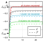
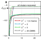
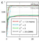
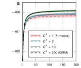
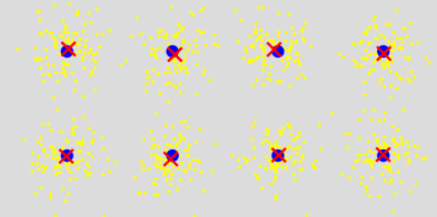
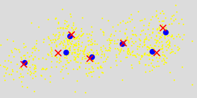
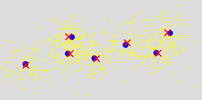
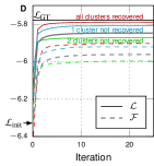
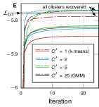
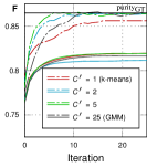
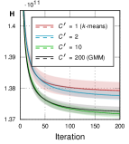
Fig. 1: A - C show results on a BIRCH data set with grid-positioned clusters, D - F on a BIRCH data set with randomly positioned clusters, and G and H on the KDD data set. The first column (plots A and D) shows log-likelihoods and free energies per data point for three individual runs of Alg. 1 ($k$-means). Red: all of the 25 clusters are found correctly; Blue: all but one; Green: all but two cluster. Additionally, the ‘grey’ plot shows the mean of 100 independent runs. Plots B and E each show the mean log-likelihood (solid line) and the log-likelihood of the run with the highest final value (striped) based on 100 runs of Alg. 3 ($k$-means-$C^{\prime}$) for different $C^{\prime}$. Plots C and F show the same for the purity, where we show the run with the highest sum of purity and NMI (additional plots for the NMI are given in Fig. S2). For comparison, we show results for DBSCAN, with free parameters optimized for highest combined purity and NMI. For BIRCH with random clusters, DBSCAN reaches a purity of $0.5$, which is hence not visible in plot F. Detailed results including comparisons with lazy-$k$-means, are given in Suppl. E. Plot G shows the mean log-likelihood and free energy (shaded with their respective SEMs) of $k$-means-$C^{\prime}$ (Alg. 3) with different $C^{\prime}$ based on 10 individual runs each. H visualizes the same runs but plots the quantization error instead. Visualizations of some ground truth cluster centers (blue circles) and found cluster centers of the best runs (red crosses) are shown in I ($k$-means, BIRCH $5\times 5$ grid), J ($k$-means, BIRCH $25\,\times$ random) and K ($k$-means-$C^{\prime}$ with $C^{\prime}=2$ on BIRCH $25\,\times$ random).

Alg. 3 ($k$-means-$C^{\prime}$), for which Prop. 4 applies, can be compared to soft-$k$-means (MacKay, 2003), which was suggested as a ‘non-hard’ $k$-means generalization. Soft-$k$-means and $k$-means-$C^{\prime}$ share an additional parameter for data variance. For $k$-means-$C^{\prime}$ this is the variance $\sigma^{2}$ itself, for soft-$k$-means this parameter is the ‘stiffness’ parameter $\beta$, which also closely links to $\sigma^{2}$ (essentially $\beta=\frac{1}{2\sigma^{2}}$) of GMM (2). However, $k$-means-$C^{\prime}$ makes $k$-means ‘softer’ by allowing for more than one non-zero value for the cluster assignments. This is different from soft-$k$-means, which maintains non-zero values for all cluster assignments. Related to this, problems with sensitivity to stiffness values and sensitivity to initial conditions compared to standard $k$-means (Barbakh and Fyfe, 2008) may be related to Prop. 1 and Prop. 2 which imply that for any approach with $C^{\prime}>1$, updates of $\sigma^{2}$ should (in contrast to soft-$k$-means) not be neglected. $k$-means-$C^{\prime}$ is itself closely related to the GMM algorithms of Shelton et al. (2014) and Hughes and Sudderth (2016). But while Shelton et al. (2014) and Hughes and Sudderth (2016) focus on EM acceleration, no proofs that their algorithms monotonically increase free energies are given (we elaborate in Suppl. C).

In general, other selection criteria than (8) could be derived for other mixture models. Visa versa also other versions of $k$-means based on other criteria than (8) can be interpreted as variational EM. An example is lazy-$k$-means which is a relatively recent $k$-means generalization used to study convergence properties (Har-Peled and Sadri, 2005). Lazy-$k$-means only reassigns a data point $n$ from a cluster $\tilde{c}$ to a new cluster $c$ if:

$$(1+\epsilon)\,\|{}\vec{y}^{\,(n)}\,-\,\vec{\mu}_{c}\|{}\,<\,\|{}\vec{y}^{\,(n)}\,-\,\vec{\mu}_{\tilde{c}}\|{}\,,$$ (21)

where $\epsilon\geq{}0$ is small, and $k$-means is recovered for $\epsilon=0$.

By considering Prop. 1, any replacement of states in ${\cal K}$ according to (21) would also increase the free energy (7). Based on our variational interpretation, lazy-$k$-means corresponds to a partial TV-E-step. In analogy to Prop. 1, we can show that (7) is monotonically increased, but it is not necessarily maximized, i.e., Corollary 1 does not apply. However, the essential observation of a decoupled $\vec{\mu}$ and $\sigma^{2}$ update only depends on $C^{\prime}$ being equal to one. Prop. 2 thus generalizes to the lazy-$k$-means case, and the same applies for Corollary 2 (see Suppl. D for the proofs). For lazy-$k$-means, polynomial running time bounds could be derived (Har-Peled and Sadri, 2005). By virtue of Corollary 2, this means that the corresponding log-likelihood bound can be optimized in polynomial time. More generally, Corollary 2 (as well as the other results) can serve for transferring many of the diverse run-time complexity results for $k$-means and $k$-means-like algorithms to results for GMM bounds. Likelihood bounds are, on the other hand, of interest for theoretical studies of GMM optimization (e.g. Kalai et al., 2010; Moitra and Valiant, 2010; Xu et al., 2016). The here established link can thus serve to transfer results from $k$-means-like approaches (e.g. Arthur et al., 2009) to GMM clustering.

In this study, we have focused on $k$-means and its relation to GMMs with isotropic Gaussians and equal mixing proportions (Eqn. 2). The analytical tools applied here could be used similarly for general GMM densities. Also in the general case it would be possible to define algorithms only considering the $C^{\prime}$ most relevant clusters for updates. However, the criterion to assign clusters to data points would diverge considerably from the closest cluster selection used by $k$-means. As a consequence, even when choosing $C^{\prime}$=$1$, a general GMM density would not result in a decoupling of $\vec{\mu}_{c}$ updates from the updates of the other model parameters. We elaborate in Suppl. C.

Finally, a very popular $k$-means version is fuzzy $k$-means (e.g., Bezdek, 1981, for references), which takes the form of a generalization of the $k$-means objective (1) by using non-binary $s_{c}^{(n)}$ in the place of the $k$-means assignments. Fuzzy $k$-means algorithms then update weighted cluster assignments and cluster centers in order to minimize such objectives. Prop. 4 serves best to highlight the differences between standard fuzzy $k$-means and $k$-means-$C^{\prime}$, because it shows that the average entropy of the cluster assignments emerges in the context of GMMs as a term in addition to a softened objective. Standard algorithms for fuzzy $k$-means (e.g. Bezdek, 1981; Yang, 1993) are different as they usually generalize the $k$-means objective without an additional entropy term. Notably, newer versions of fuzzy $k$-means have been suggested to improve on earlier versions by introducing additional regularization terms. One of these regularizations takes the form of the entropy of cluster assignments (compare Miyamoto et al., 2008, Sec. 2). Considering Eqn. 20 of Prop. 4, we could now relate the regularization constant of entropy regularized fuzzy $k$-means to the GMM log-likelihood optimization, or introduce novel versions of fuzzy $k$-means with many weights set to ‘hard’ zeros. Other, e.g., quadratic regularizations (see Miyamoto et al., 2008) are, on the other hand, not as closely related to the GMM objective but may correspond to other data statistics.

5 Numerical Verification

Before we conclude, we briefly numerically verify the main theoretical results of this work. We use a BIRCH dataset with $C=25$ clusters on a $5\times{}5$ grid with $N=100$ data points per cluster (same data set for all runs) as partly shown in Fig. 1I. Fig. 1A shows different runs of standard $k$-means and the time course of the free energy and likelihood computed using (15) and (3), respectively. The shown exemplary runs converge to different optima. The run with highest final free energy recovers all cluster centers and results in a log-likelihood larger than the log-likelihood of the generating (ground-truth) parameters. We verified that this (small) overfitting effect decreases with increasing $N$. The bound for the best run is relatively tight, which is consistent with (16) of Prop. 3 for small $\sigma^{2}$. The gap is larger for local optima, which have to have a larger $\sigma^{2}$ according to (14) and consequently higher entropy for $q_{c}^{(n)}$ of $C^{\prime}>1$ including $C^{\prime}=C$. The gap also increases for clusters with larger overlap in Fig. 1D/J, where we use the same setting as for Fig. 1A but with randomly (uniformly) distributed cluster centers (see Fig. 1J and 1K). Note that we use the seeding of $k$-means++ (Arthur and Vassilvitskii, 2006) for Fig. 1. The initial values of ${\cal L}(\Theta)$ are thus already relatively high (see ${\cal L}_{\text{init}}$).

Fig. 1E shows different runs of $k$-means-$C^{\prime}$ for the data as used for Fig. 1J. Using $k$-means-$C^{\prime}$ with different numbers of winning clusters $C^{\prime}$ can prevent shifted cluster centers caused by unsymmetrical cluster overlaps (compare Fig. 1J and 1K). Final likelihoods of the best runs with $C^{\prime}>1$ can hence be higher than those for $k$-means. Fig. 1E,J,K can also serve as numerical verification of the differences between free energies for different $C^{\prime}$. Suppl. E elaborates on this. Figs. 1C/F give additional results on the purity. Here we also compare to the popular DBSCAN method (Ester et al., 1996). While for the well separated grid data set the purity is comparably high, for the random set with larger overlaps, the purity for DBSCAN is with around 0.5 no longer comparable. More detailed results are given in Tab. S1, where we also show results for lazy-$k$-means. Finally, Figs. 1G and H verify our results using real and large scale data. The KDD-Cup 2004 Protein Homology Task (KDD, Caruana et al., 2004) comprises 145 751 samples of 74-dimensional data points. We observe tighter bounds between log-likelihood (3) and free energy (7) for better solutions of increasing $C^{\prime}$. Already for $C^{\prime}=2$ the $D_{KL}$-gap decreases significantly relative to $k$-means and vanishes nearly completely for $C^{\prime}=10$.

6 Conclusion

We have established a novel and, we believe, very natural link between $k$-means and EM for GMMs by showing that $k$-means is a special case of a truncated variational EM approximations for GMMs. The link can serve to transfer theoretical research between $k$-means-like and GMM clustering approaches (Sec. 4 treated some examples). Of the many studies which consider $k$-means and data samples of GMMs (e.g. Chaudhuri et al., 2009, & refs. therein), there is none that provides the close theoretical links and free energy results provided here (also see Suppl. B). Earlier work by Pollard (1982) is maybe one of the most relevant studies, as it proves a theorem which relates the convergence points of $k$-means to an underlying distribution. In the sense of a central limit theorem, this distribution is given by a GMM with clusters of specific covariance. Cluster overlap in the samples influences the cluster shapes via non-zero off-diagonal elements. The question of Pollard (1982) is thus how to fit a GMM (in a central limit theorem sense) to correspond to $k$-means convergence points. Prop. 3 may be related to the theorem of Pollard (1982) but a closer inspection would require a more extensive analysis.

Other than the above discussed theoretical link of $k$-means to GMM clustering, our investigations may also be useful for the analysis and improvement of further aspects of $k$-means-like and GMM clustering. GMMs are used to address a wide range of tasks. Two examples may be image denoising (e.g. Zoran and Weiss, 2011) and video tracking (e.g. Jepson et al., 2003; Lan et al., 2015, 2018). Training $k$-means may, however, often be more efficient, which can be of importance, e.g., when a lot of data has to be processed in short times. By assigning a probabilistic interpretation to $k$-means, it may offer itself as a faster alternative to GMMs in such settings. Similarly, $k$-means-$C^{\prime}$ could be used as a compromise between GMMs and efficient $k$-means versions. A further aspect our results can be related to is the estimation of cluster numbers. The standard $k$-means algorithm (Alg. 1), standard EM for GMMs (Alg. 2) as well as $k$-means-$C^{\prime}$ (Alg. 3) require the number of clusters as input. A large number of studies have addressed this disadvantage of the standard approaches. Model selection and fully Bayesian approaches (Fraley and Raftery, 1998; Rasmussen, 2000; Neal, 2000) are common methods to estimate the cluster numbers of GMMs from data. For $k$-means, well known contributions are the $X$-means algorithm (Pelleg et al., 2000), the $G$-means algorithm (Hamerly and Elkan, 2004) as well as approaches based on clustering stability (see von Luxburg, 2010, & refs. therein). All the approaches for $k$-means use standard $k$-means iterations or full $k$-means runs as part of the complete algorithm, e.g., as subroutines in split-and-merge approaches (Ueda et al., 2000, & refs. therein). There are different options how the results of this study can be combined with these previous studies. For $X$-means-like approaches, our results (e.g., Eqn. 14) could be used to quantify how well the BIC selection criterion used by $X$-means can be expected to work. If for a given data set $k$-means is not well approximating GMM solutions (e.g., for larger cluster overlaps), $k$-means-$C^{\prime}$ iterations would offer themselves as alternative iterations within an $X$-means setting. Less directly, $k$-means-$C^{\prime}$ algorithms could (A) be used in conjunction with statistical tests for Gaussianity of projected data as in $G$-means, or (B) they could be used (like $k$-means) to define stability scores for stability-based selections of cluster numbers. Also in these two cases, improvements can be expected especially when cluster overlaps are large. Finally, $k$-means and $k$-means-$C^{\prime}$ could be combined with general Bayesian model selection (Schwarz, 1978) as their free energies (Eqns. 19 and 20, respectively) provide likelihood approximations.

More generally, $k$-means is usually not directly integrated into probabilistic frameworks as the limit to zero cluster variance remained the most well known relation between $k$-means and GMMs. From the probabilistic point of view, this limit is unsatisfactory, however, as the likelihood of data points under a GMM with $\sigma^{2}\rightarrow{}0$ also approaches zero. Truncated approaches (which allow for a $k$-means/GMM relation with finite variances $\sigma^{2}>0$) are novel compared to standard variational approaches which assume a-posteriori independence (e.g. Saul et al., 1996; Jaakkola, 2000). Truncated EM approaches (Lücke and Eggert, 2010; Sheikh et al., 2014; Lücke, 2018) aim at scalable and accurate approximations without assuming a-posteriori independence; a goal they share with many later approaches (e.g. Mnih and Gregor, 2014; Rezende and Mohamed, 2015; Salimans et al., 2015; Kucukelbir et al., 2016). Truncated EM is a natural variational approximation for $k$-means-like algorithms, and is here not only related but becomes, indeed, identical to standard $k$-means.

Supplement

Supplementary A Illustration of truncated posterior approximations

Fig. S1 illustrates truncated distributions for an example with two-dimensional data points ($D=2$) with $C=8$ clusters. As can be observed, the truncated distributions with $C^{\prime}=3$ is capturing the posterior structure for data point $n$ well. For basically all data points (grey dots), truncated distributions with $C^{\prime}=3$ are sufficiently exact; and for most data points $C^{\prime}=2$ already represent a very good approximations. Also the case $C^{\prime}=1$, which correspond to the $k$-means case, will sufficiently well model the posterior because for most data points in this example the posterior is dominated by the value of the closest cluster. Also see Figs. S2 and S3 for numerical verifications.

Fig. S1: Illustration of truncated distributions for a GMM (2) in $D=2$ dimensions. The figure considers a data point $\vec{y}^{\,(n)}$ which lies (for illustrative purposes) to some extend in between some clusters. The full posterior (the responsibilities) $r_{c}^{(n)}=p(c\,|\,\vec{y}^{\,(n)},\Theta)$ for the $C=8$ clusters are shown in the top-left. Below, a truncated approximation $q_{c}^{(n)}$ with $|{\cal K}^{(n)}|=C^{\prime}=3$ is shown for the same data point. The truncated approximation maintains the $C^{\prime}$ highest posterior values, sets all others to zero, and renormalizes the distribution to sum to one. The three closest clusters, which correspond to the three highest posterior values, are connected with black lines in the main figure.

Supplementary B $k$-Means and hard cluster assignments for GMMs

Here we provide more details on how $k$-means or the $k$-means objective has previously been related to maximum likelihood optimization of GMMs.

Classification expectation maximization. The log-likelihood objective of GMMs (3) and the quantization error (1) optimized by $k$-means are non-trivially related. This is also the case for the GMMs with isotropic and equal Gaussian variances and equal mixing proportions as considered here (Eq. 2). For the purposes of our study we emphasize this point as earlier contributions reported results for clustering criteria from which one may incorrectly infer a trivial relation between (1) and (3). One example of such previous work (see Celeux and Govaert, 1992, and references therein) does, for instance, consider a classification expectation maximization (CEM) algorithm for clustering. The paper defines a classification maximum likelihood (CML) objective which is (in the notation of this paper) given by:

$${\cal L}^{\,\mathrm{CML}}(\Theta) =\frac{1}{N}\sum_{n=1}^{N}\sum_{c=1}^{C}s_{c}^{(n)}\log\!\Big{(}\frac{1}{C}\,{\cal N}\big{(}\vec{y}^{\,(n)};\vec{\mu}_{c},\sigma^{2}\hbox{$1\hskip-1.2pt\vrule depth=0.0pt,height=6.88889pt,width=0.7pt\vrule depth=0.0pt,height=0.3pt,width=1.19995pt$}\big{)}\Big{)},$$ (22)

where the $s_{c}^{(n)}$ are the binary weights of Alg. 1. In the paper (Celeux and Govaert, 1992) it is then shown that the problem of maximizing the CML objective (22) is equivalent to the problem of minimizing the quantization error (1). Although (22) is also referred to as a maximum likelihood (ML) objective (see Celeux and Govaert, 1992, and references therein), note the difference between this classification maximum likelihood (CML) objective (22) and the standard ML objective for GMMs in (3). Essentially, the sum over clusters in (3) and the logarithm can not be trivially commuted to obtain (22). Eq. (16) can be regarded as quantification of the difference between (22) and (3) in terms of the ratio between data-to-cluster center distances and $\sigma$ (compare initial discussion of Celeux and Govaert, 1992). Eq. (16) is ultimately a consequence of applying Jensen’s inequality to commute logarithm and the sum over clusters, which gives rise to a lower free energy bound. Only if cluster centers are far apart compared to $\sigma$, the sum over $c$ will for each data point $n$ be dominated by the terms of within cluster distances. This is the case of well separable clusters, i.e., if ‘hard’ data partitions are representing a good approximation of ‘soft’ a-posterior assignments. In that case the KL-divergence becomes zero. Also see Supplement E below for numerical experiments showing differences between the $k$-means and log-likelihood objectives.

Hard cluster assignments and variational distributions. As discussed in the main text, the by far most common approach to relate $k$-means and Gaussian mixture models is to take the limit to zero cluster variances $\sigma^{2}\rightarrow{}0$. This relation is very commonly used in text books as well as in the research literature itself. Alternatively, and related to this study, $k$-means is for didactic purposes also sometimes casually related to GMM optimization using variational EM. Such a relation is usually confined to derivations that make the relation of $k$-means to GMM data models plausible. For instance, if the free energy w.r.t. a variational distribution is in its standard form given by

$${\cal F}(q,\Theta) =\textstyle\frac{1}{N}\sum_{n=1}^{N}\Big{(}\sum_{c=1}^{C}q^{(n)}(c)\log\big{(}p(c,\vec{y}^{\,(n)}\,|\,\Theta)\big{)}$$

$$\phantom{iiiiiiiiiiiii}\textstyle\,-\,\sum_{c=1}^{C}q^{(n)}(c)\log\big{(}q^{(n)}(c)\big{)}\Big{)}$$ (23)

then one can informally define $q^{(n)}(c)$ to be equal to one if and only if $c$ corresponds to the maximal value of $q^{(n)}(c)$. For GMM (2) $q^{(n)}(c)$ are then given by:

$$q^{(n)}(c) =\left\{\begin{array}[]{cl}1&\mbox{if }\forall{}c^{\prime}\neq{}c:\|\vec{y}^{\,(n)}-\vec{\mu}_{c}\|<\|\vec{y}^{\,(n)}-\vec{\mu}_{c^{\prime}}\|\\[2.84526pt] 0&\mbox{otherwise}\end{array}\right..$$ (26)

As the entropy for such a distribution is equal to zero, the free energy reduces to

$${\cal F}(q,\Theta) =\textstyle\frac{1}{N}\sum_{n=1}^{N}\log\big{(}p(c_{o}^{(n)},\vec{y}^{\,(n)}\,|\,\Theta)\big{)}$$ (27)

where $c_{o}^{(n)}$ denotes the cluster closest to data point $\vec{y}^{\,(n)}$. $k$-means is then often taken as optimizing this objective.

In order to make any mathematically rigorous statements, the argumentation above lacks, at closer inspection, a solid theoretical foundation in two important aspects: (A) Derivations of the free energy using variational distributions all assume $q^{(n)}(c)$ to be strictly positive ($q^{(n)}(c)>0$ for all $n$ and $c$), which is violated for $q^{(n)}(c)$ defined as in Eq. (26). (B) Relating $k$-means to a free energy objective as (27) implicitly assumes the variational distributions $q^{(n)}(c)$ to be independent of the model parameters $\Theta$ (i.e., independent of $\vec{\mu}_{1:C}$ and $\sigma^{2}$ in our case). Considering Eq. (26) also this independence is not given (which is in contrast, e.g., to mean field distributions). The model parameters can also not simply be assumed to be constant as is the case for full posteriors in standard EM: The proof verifying that values for the model parameters can be held fixed is given for full posteriors only (see, e.g., Lemma 1 of Neal and Hinton, 1998) but it does not necessarily apply for general variational distributions $q^{(n)}(c)$ defined using model parameters $\Theta$.

The here applied results (Lücke, 2018) do address both these aspects: variational distributions with ‘hard’ zeros are treated (Point A), and variational distributions that can depend on the model parameters are explicitly considered (Point B). Addressing any of these two points is non-trivial (see Propositions 1 and 2 in Lücke (2018), for Point A; and, e.g., Propositions 3-5 in Lücke (2018), for Point B). However, if treated rigorously, results for a large class of distributions (which includes distributions of Eq. 26) can be derived, and the derived results apply for any generative model with discrete latents. Notably, also truncated variational distributions with non-zero entropy are included as well as distributions (26) in which $q^{(n)}(c)=1$ does not necessarily apply for the closest cluster (such distributions are important, e.g., in relation to lazy-$k$-means, see Proposition 4). In this paper we make use of results of Lücke (2018) by applying them to GMMs given by Eq. (2) (e.g., through Propositions 1 and 4 which in turn use the simplified free energy (7) of Lücke (2018)).

The difficulties to cleanly and rigorously treat distributions such as (26) may explain why (to the knowledge of the authors) any relation of $k$-means and variational approaches is rather informally discussed (compare, e.g., Jordan et al. (1997), who, e.g., relate Viterbi training to variational EM). If the relation of $k$-means to GMMs is made more explicit, the literature, including popular text books (e.g. MacKay, 2003; Barber, 2012), drops back to the zero variance limit to derive $k$-means.

Supplementary C Generalization of criterion (8) for general GMMs

Consider a general standard GMM of the form:

$$p(c\,|\,\Theta) =\pi_{c}\quad\text{with }\textstyle\sum_{c=1}^{C}\pi_{c}=1,$$ (28)

$$p(\vec{y}\,|\,c,\Theta) =|2\pi\Sigma_{c}|^{-\frac{1}{2}}\exp\!\big{(}\!-\!\textstyle\frac{1}{2}\|\vec{y}-\vec{\mu}_{c}\|^{2}_{\Sigma_{c}}\big{)},$$ (29)

$$\|\vec{y}-\vec{\mu}_{c}\|^{2}_{\Sigma_{c}} =(\vec{y}-\vec{\mu}_{c})^{\mathrm{T}}\Sigma^{-1}_{c}(\vec{y}-\vec{\mu}_{c}),$$ (30)

where $\pi_{c}\geq{}0$ are the mixing proportions, $\Sigma_{c}$ is a for each $c$ positive definite covariance matrix, and $|\cdot|$ denotes the determinant. We denote by $\Theta=(\pi_{1:C},\vec{\mu}_{1:C},\Sigma_{1:C})$ the set of all parameters. For GMM (28) to (30) a corresponding variational free energy is because of Eq. (7) (first line) increased if and only if:

$$p(c,\vec{y}\,|\,\Theta)>p({\tilde{c}},\vec{y}\,|\,\Theta)$$

$$\Leftrightarrow \textstyle\pi_{c}\,|2\pi\Sigma_{c}|^{-\frac{1}{2}}\exp\!\big{(}\!-\!\frac{1}{2}\|\vec{y}-\vec{\mu}_{c}\|^{2}_{\Sigma_{c}}\big{)}$$

$$>\; \textstyle\pi_{\tilde{c}}\,|2\pi\Sigma_{\tilde{c}}|^{-\frac{1}{2}}\exp\!\big{(}\!-\!\frac{1}{2}\|\vec{y}-\vec{\mu}_{\tilde{c}}\|^{2}_{\Sigma_{\tilde{c}}}\big{)}$$

$$\Leftrightarrow \textstyle\log(\pi_{c})-\frac{1}{2}\log(|2\pi\Sigma_{c}|)-\frac{1}{2}\|\vec{y}-\vec{\mu}_{c}\|^{2}_{\Sigma_{c}}$$

$$>\; \textstyle\log(\pi_{\tilde{c}})-\frac{1}{2}\log(|2\pi\Sigma_{\tilde{c}}|)-\frac{1}{2}\|\vec{y}-\vec{\mu}_{\tilde{c}}\|^{2}_{\Sigma_{\tilde{c}}}$$

$$\Leftrightarrow \|\vec{y}-\vec{\mu}_{c}\|^{2}_{\Sigma_{c}}+\log(|2\pi\Sigma_{c}|)-2\log(\pi_{c})$$

$$<\; \|\vec{y}-\vec{\mu}_{\tilde{c}}\|^{2}_{\Sigma_{\tilde{c}}}+\log(|2\pi\Sigma_{\tilde{c}}|)-2\log(\pi_{\tilde{c}})\,.$$ (31)

In comparison, Shelton et al. (2014) use an estimated E-step, which does consequently not guarantee a monotonic increase of a free energy. Hughes and Sudderth (2016) do use a constrained likelihood optimization to find the best $C^{\prime}$ clusters per data point (related to Corollary 1), but a complete proof for general GMMs would require Proposition 5 of Lücke (2018), which warrants that M-steps can be derived while the parameters $\Theta$ of the variational distributions $q_{c}^{(n)}$ remain fixed.

Table S1: Log-likelihood per data point $\mathcal{L}$, quantization error $\phi$, purity and normalized mutual information (NMI) for $k$-means, $k$-means-C’ with $C^{\prime}=2$, lazy-$k$-means with $\epsilon=0.1$ and DBSCAN on the BIRCH data sets. The free parameters of DBSCAN were optimized to maximize the sum of NMI and purity. Using such a combination for parameter tuning prevents settings highly overfitted to one of the two criteria with high trade-offs on the other. Given are the means over 100 independent runs as well as the values of the best single run. The mean and the best are identical for DBSCAN given the same, optimized free parameters. The best values per column are written in bold.

Algorithm	BIRCH $5\times 5$ (grid)								BIRCH ($25\,\times$ random positions)
	$\mathcal{L}$		$\phi$		$\mathrm{purity}$		$\mathrm{NMI}$		$\mathcal{L}$		$\phi$		$\mathrm{purity}$		$\mathrm{NMI}$
	mean	best	mean	best	mean	best*	mean	best*	mean	best	mean	best	mean	best*	mean	best*
$k$-means	-6.127	-6.016	5,503	4,836	0.971	0.992	0.977	0.987	-5.842	-5.789	4,535	4,291	0.819	0.856	0.879	0.875
$k$-means-C’	-6.117	-6.016	5,476	4,837	0.973	0.992	0.978	0.986	-5.828	-5.771	4,637	4,331	0.811	0.864	0.880	0.880
lazy-$k$-means	-6.117	-6.016	5,452	4,837	0.974	0.992	0.978	0.987	-5.850	-5.803	4,592	4,351	0.809	0.846	0.876	0.880
DBSCAN	–	–	–	–	0.989	0.989	0.982	0.982	–	–	–	–	0.502	0.502	0.800	0.800

*: best values for purity and NMI are for all algorithms given as values of the run with the highest sum of purity and NMI to omit solutions highly overfitted to one of the two criteria

           

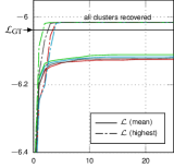
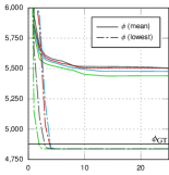
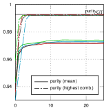
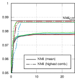
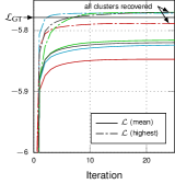
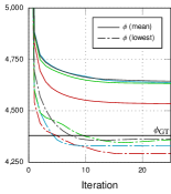
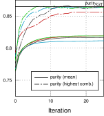
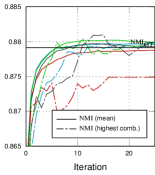
Fig. S2: The four columns show from left to right: the log-likelihood $\mathcal{L}$, quantization error $\phi$, purity, and normalized mutual information (NMI) of the $k$-means-C’ algorithms on BIRCH data sets as in Fig. 1. The plots show the mean over 100 independent runs (solid line). For the log-likelihood and quantization error, the single run with the best respective final value is shown in striped. For the purity and NMI plots, the single run with the highest sum of purity and NMI is shown in striped. Such a selection criterion omits runs that are highly overfitted to either purity or NMI.

Considering (31), note that the criterion to select clusters now depends on all model parameters (in contrast to the criterion of Eq. 8). If algorithms for parameter updates are defined based on (31), all current parameter values have to be considered in E-steps which compute generalizations of the responsibilities $q_{c}^{(n)}$ (compare Eq. 5). Notably, even if these responsibilities $q_{c}^{(n)}$ become binary for the choice $C^{\prime}=1$, the selection of the non-zero values of $q_{c}^{(n)}$ would still require the other parameter values. There would consequently not be a $k$-means-like decoupling from other parameter updates like for the GMM defined by Eq. (2).

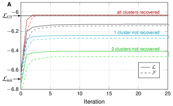
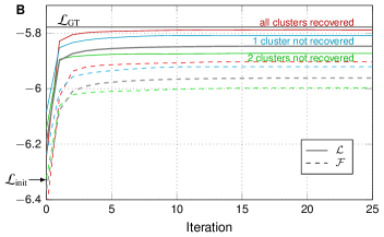
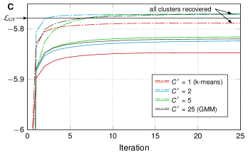
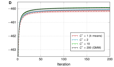
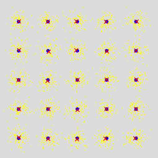
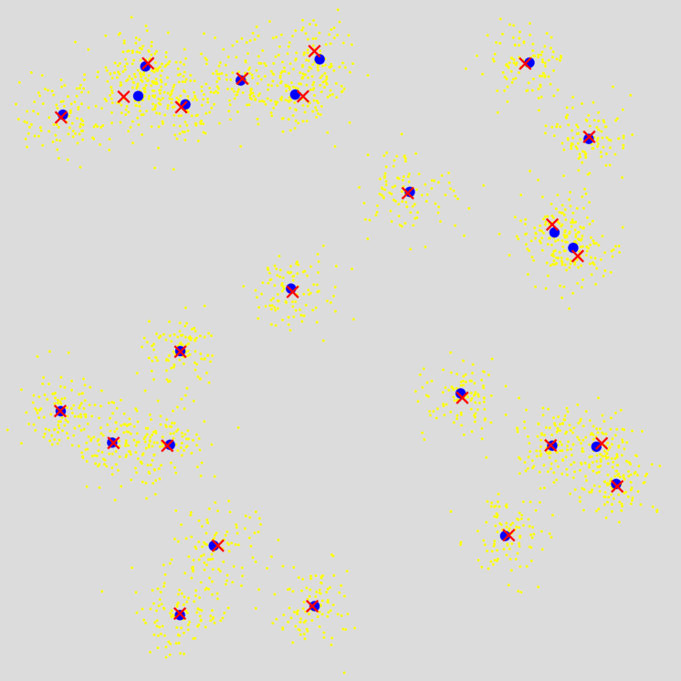
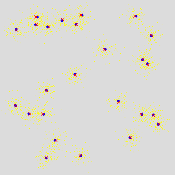
Fig. S3: A shows experiments of Alg. 1 ($k$-means) on a BIRCH data set with grid-positioned clusters, as visualized in E. Shown are the log-likelihood and free energy per iteration for three individual runs (red, blue and green) and the mean of 100 independent runs (gray). The individual runs show convergences to different optima. B shows the same experiments as A on uniform randomly positioned clusters, as visualized in F. In A and B, the $D_{KL}$-gap at convergence is visualized as colored vertical lines next to the plot and can in A be clearly observed to increase for less optimal solutions. In B, due to higher cluster overlaps, the $D_{KL}$-gap is here overall larger compared to A. C shows the mean log-likelihood (solid line) and the log-likelihood of the best run (striped) of 100 runs of Alg. 3 ($k$-means-$C^{\prime}$) for different $C^{\prime}$. For $C^{\prime}\geq 2$, the best solutions are close to identical for the different settings, although some tend to find these best solutions more frequently. D shows the mean log-likelihood (solid line) and free energy (dashed) on the KDD data set over 10 runs, shaded with their respective SEMs. Visualization of some ground truth cluster centers (blue circles) and found cluster centers of the best runs (red crosses) on BIRCH data sets are shown in E, F (for $k$-means) and G (for $k$-means-$C^{\prime}$ with $C^{\prime}=2$). Comparison of F and G shows the difference between using $C^{\prime}=1$ ($k$-means) and $C^{\prime}>1$. Especially for regions with higher cluster overlap, $k$-means tends to push close-by clusters away from each other, due to the hard assignment of data points to only a single cluster. This effect can be observed on the groups of two and three clusters in the upper half as well as on the group of clusters in the bottom left corner. For $C^{\prime}=2$, this effect is already greatly reduced.

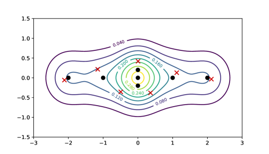
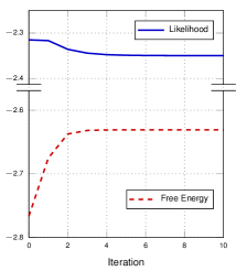
(a) $k$-means

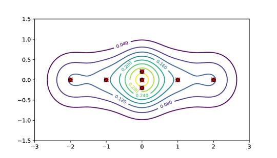
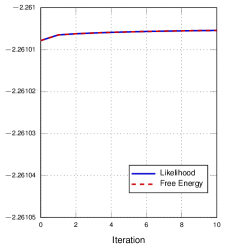
(b) GMM

Fig. S4: This example illustrates that the free energy and the GMM likelihood objective are not trivially related. We generate data from seven overlapping, equal and isotropic Gaussians arranged as above (black circles), drawing 100 000 data samples per Gaussian. The contour lines show the underlying probability density distribution of which the data points are drawn. We compare $k$-means in (a) with EM for isotropic (non-truncated) GMMs in (b). For both, we use the ground-truth generating cluster centers (and variances for the GMM) as initialization. If we now run $k$-means, we observe that while the free energy increases the log-likelihood decreases. For this example the final cluster centers (red crosses) obtained by $k$-means differ very significantly from the ground-truth. But also, e.g., for just two overlapping Gaussians, $k$-means results in final cluster centers significantly different from ground truth as can be observed in Fig. S3 (F/G). The higher the cluster overlap, the more pronounced this effect becomes. EM for GMM does on the other hand (as expected) result in final cluster centers (red crosses) very similar to ground truth (note the different scales of the plots; the higher initial likelihood value for the GMM compared to $k$-means is not due to different initial cluster centers, but due to a different $\sigma^{2}$-value for $k$-means as a result of applying Eq. (14) with $k$-means activations). Our example also provides a counterexample for the $k$-means objective (1) and the likelihood objective for GMMs (3) giving rise to the same optimization problem: here, the quantization error decreases, but the GMM likelihood gets worse. The optimization of equally sized, isotropic GMMs (2) and of the $k$-means objective are sometimes regarded as equivalent; Feldman et al. (2011), for instance, write “[…] their result requires that the Gaussians are identical spheres, in which case the maximum likelihood problem is identical to the $k$-means problem”. Also results of Pollard (1982), who is often cited for showing that $k$-means is a GMM maximum likelihood estimator, seem to be misinterpreted sometimes. $k$-means becomes an increasingly good maximum likelihood estimator if we additionally demand increasingly separable clusters. Increased separability is in turn closely related to the $\sigma^{2}\rightarrow{}0$ limit, in which the $k$-means and GMM objectives become increasingly similar.
Feldman, D., Faulkner, M., Krause, A., 2011, Scalable training of mixture models via coresets, NIPS, 2142–2150.
Pollard, D., 1982. A central limit theorem for k-means clustering. The Annals of Probability, 919–926.

Supplementary D Generalizations for lazy-$k$-means

If we change the cluster selection criterion (8) to the criterion for lazy-$k$-means (21), then it follows from Proposition 1 that each cluster assignment in lazy-$k$-means increases the free energy (7). As the M-steps (equal to the $k$-means M-steps) then increase the free energy w.r.t. $\Theta$, it follows that lazy-$k$-means monotonically increases the same free energy objective. Corollary 1 does not apply but we can generalize Proposition 2.

Proposition (Generalization of Proposition 2 for lazy-$k$-means)
Consider the TV-EM algorithm (Alg. 3) but with criterion (21) instead of criterion (8). If we set $C^{\prime}=1$, then the TV-EM updates of the cluster centers $\vec{\mu}_{c}$ (6) become independent of the variance $\sigma^{2}$ and are given by the lazy-$k$-means algorithm.
Proof
The proof is analogous to the one of Proposition 2 with the only difference that $c_{o}^{(n)}$ is now a cluster of $\vec{y}^{\,(n)}$ for which applies: $\forall\tilde{c}\neq{}c_{o}^{(n)}:\|\vec{y}^{\,(n)}\,-\,\vec{\mu}_{c_{o}^{(n)}}\|<(1+\epsilon)\,\|\vec{y}^{\,(n)}\,-\,\vec{\mu}_{\tilde{c}{}}\|$. The cluster assignments thus become those of lazy-$k$-means, while the parameter updates remain those of standard $k$-means (i.e., the same as used for lazy-$k$-means).
$\square$
As Propositions 1 and 2 can be generalized, the fact that lazy-$k$-means optimizes the same free energy as $k$-means does also imply that Corollary 2 can be used to relate lazy-$k$-means to the GMM objective (3).

Supplementary E More details on the numerical experiments

Fig. S2 shows additional results of $k$-means-$C^{\prime}$ on the BIRCH data sets, namely the log-likelihood, quantization error, purity and NMI (where likelihood and purity values are the same as those in Fig. 1, but shown here again for easier comparison). Tab. S1 gives a numerical comparison of these results to the DBSCAN and lazy-$k$-means algorithms. The results on the quantization error compared to the likelihoods in Fig. S2 and Tab. S1 highlight the fact that optimization of the $k$-means criterion (i.e., the quantization error) does generally not directly coincide with optimization of free energies by $k$-means-$C^{\prime}$ with $C^{\prime}>1$ (including optimization of likelihoods by EM for GMM for $C^{\prime}=C$). For the NMI and purity scores, we find that on the BIRCH set with random clusters (and therefore larger overlaps) $k$-means is prone to trade off NMI with decreasing purity scores (which results in a lower than average NMI score for the shown run with the highest combined score of NMI and purity). The $k$-means-$C^{\prime}$ algorithm, on the other hand, already results for $C^{\prime}=2$ in high NMI and purity scores near the ground truth.

Fig. S3 shows enlarged versions of plots A, D, E, G of Fig. 1 with more details in the caption. In addition to these results we also verified that the free energies (7), (15) and the right-hand-side of (19) are numerically equal for $k$-means. For $k$-means-$C^{\prime}$ we verified that free energies (7) and (20) are equal at convergence.

Note that Fig. S3 can also be interpreted as numerically verifying that the free energies and the likelihood objective of the GMM (2) are not trivially related. This includes the free energy (15) which is optimized by $k$-means and which corresponds to $C^{\prime}=1$. Comparison of the means of Figs. S3(F) and (G) already shows the difference when comparing results between $C^{\prime}=1$ ($k$-means) to $C^{\prime}=2$. Finally, the numerical experiment of Fig. S4 is deliberately chosen to highlight the difference between the $k$-means objective (1) and the GMM log-likelihood (3). By applying $k$-means, the $k$-means free energy increases (the quantization error gets smaller) but the log-likelihood gets worse. Results for the cluster centers recovered by $k$-means and EM for GMM (2) are very different.

References

- Allahverdyan and Galstyan (2011) Allahverdyan, A., Galstyan, A., 2011. Comparative analysis of Viterbi training and maximum likelihood estimation for HMMs, in: NIPS, pp. 1674–1682.
- Anderberg (1973) Anderberg, M.R., 1973. Cluster Analysis for Applications. Academic Press.
- Arthur et al. (2009) Arthur, D., Manthey, B., Röglin, H., 2009. k-means has polynomial smoothed complexity, in: IEEE Symp. Foundations of Comp. Sci., pp. 405–414.
- Arthur and Vassilvitskii (2006) Arthur, D., Vassilvitskii, S., 2006. How slow is the k-means method?, in: Comp. Geo., pp. 144–153.
- Bachem et al. (2016) Bachem, O., Lucic, M., Hassani, H., Krause, A., 2016. Fast and provably good seedings for k-means, in: NIPS, pp. 55–63.
- Barbakh and Fyfe (2008) Barbakh, W., Fyfe, C., 2008. Online clustering algorithms. International Journal of Neural Systems 18, 185–194.
- Barber (2012) Barber, D., 2012. Bayesian reasoning and machine learning. Cam. Univ. Press.
- Belkin and Sinha (2010) Belkin, M., Sinha, K., 2010. Polynomial learning of distribution families, in: Symp. Comp. Sci., pp. 103–112.
- Berkhin (2006) Berkhin, P., 2006. A survey of clustering data mining techniques, in: Grouping multidimensional data. Springer, pp. 25–71.
- Bezdek (1981) Bezdek, J.C., 1981. Pattern recognition with fuzzy objective function algorithms. Springer.
- Broderick et al. (2013) Broderick, T., Kulis, B., Jordan, M., 2013. Mad-bayes: Map-based asymptotic derivations from bayes, in: ICML, pp. 226–234.
- Caruana et al. (2004) Caruana, R., Joachims, T., Backstrom, L., 2004. KDD-Cup 2004: results and analysis. ACM SIGKDD Explorations Newsletter 6, 95–108.
- Celeux and Govaert (1992) Celeux, G., Govaert, G., 1992. A classification EM algorithm for clustering and two stochastic versions. Comp. statistics & Data analysis 14, 315–332.
- Chaudhuri et al. (2009) Chaudhuri, K., Dasgupta, S., Vattani, A., 2009. Learning mixtures of gaussians using the k-means algorithm. arXiv preprint arXiv:0912.0086 .
- Dai and Lücke (2014) Dai, Z., Lücke, J., 2014. Autonomous document cleaning – A Generative Approach to Reconstruct Strongly Corrupted Scanned Texts. IEEE Trans. on Pattern Analysis and Machine Intelligence 36, 1950–1962.
- Dempster et al. (1977) Dempster, A.P., Laird, N.M., Rubin, D.B., 1977. Maximum likelihood from incomplete data via the EM algorithm. J. Roy. Stat. Soc. B 39, 1–38.
- Duda et al. (2001) Duda, R.O., Hart, P.E., Stork, D.G., 2001. Pattern Classification. Wiley-Interscience (2nd Edition).
- Ester et al. (1996) Ester, M., Kriegel, H.P., Sander, J., Xu, X., et al., 1996. A density-based algorithm for discovering clusters in large spatial databases with noise., in: Kdd, pp. 226–231.
- Forster et al. (2018) Forster, D., Sheikh, A.S., Lücke, J., 2018. Neural simpletrons: Learning in the limit of few labels with directed generative networks. Neural computation , 2113–2174.
- Fraley and Raftery (1998) Fraley, C., Raftery, A.E., 1998. How many clusters? Which clustering method? Answers via model-based cluster analysis. The computer journal 41, 578–588.
- Hamerly and Elkan (2004) Hamerly, G., Elkan, C., 2004. Learning the k in k-means, in: Proc. NIPS, pp. 281–288.
- Har-Peled and Sadri (2005) Har-Peled, S., Sadri, B., 2005. How fast is the k-means method? Algorithmica 41, 185–202.
- Hoffman et al. (2013) Hoffman, M.D., Blei, D.M., Wang, C., Paisley, J.W., 2013. Stochastic variational inference. JMLR 14, 1303–1347.
- Hughes and Sudderth (2016) Hughes, M.C., Sudderth, E.B., 2016. Fast learning of clusters and topics via sparse posteriors. preprint arXiv:1609.07521 .
- Inaba et al. (2000) Inaba, M., Katoh, N., Imai, H., 2000. Variance-based k-clustering algorithms by Voronoi diagrams and randomization. Trans. Inf. Sys. 83, 1199–1206.
- Jaakkola (2000) Jaakkola, T., 2000. Tutorial on variational approximation methods, in: Opper, M., Saad, D. (Eds.), Advanced mean field methods. MIT Press.
- Jain (2010) Jain, A.K., 2010. Data clustering: 50 years beyond k-means. Pattern Recognition Letters 31, 651–666.
- Jepson et al. (2003) Jepson, A.D., Fleet, D.J., El-Maraghi, T.F., 2003. Robust online appearance models for visual tracking. IEEE Trans. on Pattern Analysis and Machine Intelligence 25, 1296–1311.
- Jordan et al. (1997) Jordan, M.I., Ghahramani, Z., Saul, L.K., 1997. Hidden markov decision trees, in: NIPS, pp. 501–507.
- Kalai et al. (2010) Kalai, A.T., Moitra, A., Valiant, G., 2010. Efficiently learning mixtures of two gaussians, in: Proc. ACM Symp. Theo. Comp., ACM. pp. 553–562.
- Kucukelbir et al. (2016) Kucukelbir, A., Tran, D., Ranganath, R., Gelman, A., Blei, D.M., 2016. Automatic differentiation variational inference. CoRR abs/1603.00788.
- Kulis and Jordan (2012) Kulis, B., Jordan, M.I., 2012. Revisiting k-means: New algorithms via Bayesian nonparametrics, in: ICML, ACM. pp. 513–520.
- Lan et al. (2015) Lan, X., Ma, A.J., Yuen, P.C., Chellappa, R., 2015. Joint sparse representation and robust feature-level fusion for multi-cue visual tracking. IEEE Transactions on Image Processing 24, 5826–5841.
- Lan et al. (2018) Lan, X., Zhang, S., Yuen, P.C., Chellappa, R., 2018. Learning common and feature-specific patterns: A novel multiple-sparse-representation-based tracker. IEEE Transactions on Image Processing 27, 2022–2037.
- Lloyd (1982) Lloyd, S., 1982. Least squares quantization in PCM. IEEE Trans. Inf. Theory 28, 129–137.
- Lücke (2018) Lücke, J., 2018. Truncated variational expectation maximization. arXiv:1610.03113 .
- Lücke and Eggert (2010) Lücke, J., Eggert, J., 2010. Expectation truncation and the benefits of preselection in training generative models. JMLR 11, 2855–900.
- Lücke and Henniges (2012) Lücke, J., Henniges, M., 2012. Closed-form entropy limits, in: AISTATS, pp. 731–740.
- von Luxburg (2010) von Luxburg, U., 2010. Clustering stability: an overview. Foundations and Trends in Machine Learning 2, 235–274.
- MacKay (2003) MacKay, D.J.C., 2003. Information Theory, Inference, and Learning Algorithms. Cambridge Univ. Press.
- McLachlan and Basford (1988) McLachlan, G.J., Basford, K.E., 1988. Mixture models: Inference and applications to clustering. volume 84. Marcel Dekker.
- Miyamoto et al. (2008) Miyamoto, S., Ichihashi, H., Honda, K., 2008. Algorithms for fuzzy clustering. Springer.
- Mnih and Gregor (2014) Mnih, A., Gregor, K., 2014. Neural variational inference and learning in belief networks, in: Proceedings of The 31st ICML.
- Moitra and Valiant (2010) Moitra, A., Valiant, G., 2010. Settling the polynomial learnability of mixtures of Gaussians, in: IEEE Symp. Found. Comp. Sci, pp. 93–102.
- Neal and Hinton (1998) Neal, R., Hinton, G., 1998. A view of the EM algorithm that justifies incremental, sparse, and other variants, in: Learning in Graphical Models, Kluwer.
- Neal (2000) Neal, R.M., 2000. Markov chain sampling methods for dirichlet process mixture models. Journal of Computational and Graphical Statistics 9, 249–265.
- Van den Oord and Schrauwen (2014) Van den Oord, A., Schrauwen, B., 2014. Factoring variations in natural images with deep Gaussian mixture models, in: NIPS, pp. 3518–3526.
- Pelleg et al. (2000) Pelleg, D., Moore, A.W., et al., 2000. X-means: Extending k-means with efficient estimation of the number of clusters., in: Proc. ICML, pp. 727–734.
- Pollard (1982) Pollard, D., 1982. A central limit theorem for -means clustering. The Annals of Probability 10, 919–926.
- Rasmussen (2000) Rasmussen, C.E., 2000. The infinite gaussian mixture model, in: Proc. NIPS, pp. 554–560.
- Rezende and Mohamed (2015) Rezende, D.J., Mohamed, S., 2015. Variational inference with normalizing flows. ICML .
- Salimans et al. (2015) Salimans, T., Kingma, D., Welling, M., 2015. Markov chain monte carlo and variational inference: Bridging the gap. ICML .
- Saul et al. (1996) Saul, L.K., Jaakkola, T., Jordan, M.I., 1996. Mean field theory for sigmoid belief networks. Journal of artificial intelligence research 4, 61–76.
- Schwarz (1978) Schwarz, G., 1978. Estimating the dimension of a model. The annals of statistics 6, 461–464.
- Segal et al. (2002) Segal, E., Battle, A., Koller, D., 2002. Decomposing gene expression into cellular processes, in: Pacific Symposium on Biocomputing, pp. 89–100.
- Sheikh et al. (2014) Sheikh, A.S., Shelton, J.A., Lücke, J., 2014. A truncated EM approach for spike-and-slab sparse coding. JMLR 15, 2653–2687.
- Shelton et al. (2014) Shelton, J.A., Gasthaus, J., Dai, Z., Lücke, J., Gretton, A., 2014. GP-select: Accelerating em using adaptive subspace preselection. arXiv:1412.3411, now published by Neural Computation 29(8):2177-2202, 2017 .
- Steinley (2006) Steinley, D., 2006. K-means clustering: A half-century synthesis. Brit. J. Math. and Stat. Psych. 59, 1–34.
- Ueda et al. (2000) Ueda, N., Nakano, R., Ghahramani, Z., Hinton, G.E., 2000. Split and merge em algorithm for improving gaussian mixture density estimates. J. of VLSI Sig. Proc. Systems for Signal, Image and Video Tech. 26, 133–140.
- Welling and Kurihara (2006) Welling, M., Kurihara, K., 2006. Bayesian k-means as a “maximization-expectation” algorithm, in: Proc. SIAM Conf. Data Mining, pp. 474–478.
- Xu et al. (2016) Xu, J., Hsu, D.J., Maleki, A., 2016. Global analysis of expectation maximization for mixtures of two gaussians, in: NIPS, pp. 2676–2684.
- Yang (1993) Yang, M.S., 1993. A survey of fuzzy clustering. Mathematical and Computer modelling 18, 1–16.
- Zoran and Weiss (2011) Zoran, D., Weiss, Y., 2011. From learning models of natural image patches to whole image restoration, in: Proc. ICCV, IEEE. pp. 479–486.