Outward Influence and Cascade Size Estimation
in Billion-scale Networks

Abstract.

Estimating cascade size and nodes’ influence is a fundamental task in social, technological, and biological networks. Yet this task is extremely challenging due to the sheer size and the structural heterogeneity of networks. We investigate a new influence measure, termed outward influence (OI), defined as the (expected) number of nodes that a subset of nodes $S$ will activate, excluding the nodes in $S$. Thus, OI equals, the de facto standard measure, influence spread of $S$ minus $|S|$. OI is not only more informative for nodes with small influence, but also, critical in designing new effective sampling and statistical estimation methods.

Based on OI, we propose SIEA/SOIEA, novel methods to estimate influence spread/outward influence at scale and with rigorous theoretical guarantees. The proposed methods are built on two novel components 1) IICP an important sampling method for outward influence; and 2) RSA, a robust mean estimation method that minimize the number of samples through analyzing variance and range of random variables. Compared to the state-of-the art for influence estimation, SIEA is $\Omega(\log^{4}n)$ times faster in theory and up to several orders of magnitude faster in practice. For the first time, influence of nodes in the networks of billions of edges can be estimated with high accuracy within a few minutes. Our comprehensive experiments on real-world networks also give evidence against the popular practice of using a fixed number, e.g. 10K or 20K, of samples to compute the “ground truth” for influence spread.

1. Introduction

In the past decade, a massive amount of data on human interactions has shed light on various cascading processes from the propagation of information and influence (Kempe et al., 2003) to the outbreak of diseases (Leskovec et al., 2007). These cascading processes can be modeled in graph theory through the abstraction of the network as a graph $G=(V,E)$ and a diffusion model that describes how the cascade proceeds into the network from a prescribed subset of nodes. A fundamental task in analyzing those cascades is to estimate the cascade size, also known as influence spread in social networks. This task is the foundation of the solutions for many applications including viral marketing (Kempe et al., 2003; Tang et al., 2014, 2015; Nguyen et al., 2016b), estimating users’ influence (Du et al., 2013; Lucier et al., 2015), optimal vaccine allocation (Preciado et al., 2013), identifying critical nodes in the network (Dinh and Thai, 2015), and many others. Yet this task becomes computationally challenging in the face of the nowadays social networks that may consist of billions of nodes and edges.

Most of the existing work in network cascades uses stochastic diffusion models and estimates the influence spread through sampling (Kempe et al., 2003; Cohen et al., 2014; Dinh and Thai, 2015; Tang et al., 2015; Lucier et al., 2015; Ohsaka et al., 2016). The common practice is to use a fixed number of samples, e.g. 10K or 20K (Kempe et al., 2003; Tang et al., 2015; Cohen et al., 2014; Ohsaka et al., 2016), to estimate the expected size of the cascade, aka influence spread. Not only is there no single sample size that works well for all networks of different sizes and topologies, but those approaches also do not provide any accuracy guarantees. Recently, Lucier et al. (Lucier et al., 2015) introduced INFEST, the first estimation method that comes with accuracy guarantees. Unfortunately, our experiments suggest that INFEST does not perform well in practice, taking hours on networks with only few thousand nodes. Will there be a rigorous method to estimate the cascade size in billion-scale networks?

$S$	Influence $\mathbb{I}(S)$	Outward Inf. $\mathbb{I}_{out}(S)$
$\{u\}$	$1+p+2p^{2}=1.12$	$p+2p^{2}=0.12$
$\{v\}$	$1+2p=1.20$	$2p=0.20$
$\{w\}$	$1.00$	$0.00$

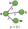
Figure 1. Left: the influence of nodes under IC model. The influence of all nodes are roughly the same, despite that $w$ is much less influential than $u$ and $v$. Right: Outward influence is better at reflecting the relative influence of the nodes. $w$ has the least outward influence, $0$, while $v$’s is nearly twice as that of $u$

In this paper, we investigate efficient estimation methods for nodes’ influence under stochastic cascade models (Daley et al., 2001; Kempe et al., 2003; Du et al., 2013). First, we introduce a new influence measure, called outward influence and defined as $\mathbb{I}_{out}(S)=\mathbb{I}(S)-|S|$, where $\mathbb{I}(S)$ denotes the influence spread. The new measure excludes the self-influence artifact in influence spread, making it more effective in comparing relative influence of nodes. As shown in Fig. 1, the influence spread of the nodes are roughly the same, $1$. In contrast, the outward influence of nodes $u,v$ and $w$ are $0.12,0.20$, and $0.00$, respectively. Those values correctly reflect the intuition that $w$ is the least influential nodes and $v$ is nearly twice as influential as $u$.

More importantly, the outward influence measure inspires novel methods, termed SIEA/SOIEA, to estimate influence spread/outward influence at scale and with rigorous theoretical guarantees. Both SOIEA and SIEA guarantee arbitrary small relative error with high probability within an $O(n)$ observed influence. The proposed methods are built on two novel components 1) IICP an important sampling method for outward influence; and 2) RSA, a robust mean estimation method that minimize the number of samples through analyzing variance and range of random variables. IICP focuses only on non-trivial cascades in which at least one node outside the seed set must be activated. As each IICP generates cascades of size at least two and outward influence of at least one, it leads to smaller variance and much faster convergence to the mean value. Under the well-known independent cascade model (Kempe et al., 2003), SOIEA is $\Omega(\log^{4}n)$ times faster than the state-of-the-art INFEST (Lucier et al., 2015) in theory and is four to five orders of magnitude faster than both INFEST and the naive Monte-Carlo sampling. For other stochastic models, such as continuous-time diffusion model (Du et al., 2013), LT model (Kempe et al., 2003), SI, SIR, and variations (Daley et al., 2001), RSA can be applied directly to estimate the influence spread, given a Monte-Carlo sampling procedure, or, better, with an extension of IICP to the model.

Our contributions are summarized as follows.

• We introduce a new influence measure, called Outward Influence which is more effective in differentiating nodes’ influence. We investigate the characteristics of this new measure including non-monotonicity, submodularity, and #P-hardness of computation.

• Two fully polynomial time randomized approximation schemes (FPRAS) SIEA and SOIEA to provide $(\epsilon,\delta)$-approximate for influence spread and outward influence with only an $O(n)$ observed influence in total. Particularly, SOIEA, our algorithm to estimate influence spread, is $\Omega(\log^{4}n)$ times faster than the state-of-the-art INFEST (Lucier et al., 2015) in theory and is four to five orders of magnitude faster than both INFEST and the naive Monte-Carlo sampling.

• The robust mean estimation algorithm, termed RSA, a building block of SIEA, can be used to estimate influence spread under other stochastic diffusion models, or, in general, mean of bounded random variables of unknown distribution. RSA will be our favorite statistical algorithm moving forwards.

• We perform comprehensive experiments on both real-world and synthesis networks with size up to 65 million nodes and 1.8 billion edges. Our experiments indicate the superior of our algorithms in terms of both accuracy and running time in comparison to the naive Monte-Carlo and the state-of-the-art methods. The results also give evidence against the practice of using a fixed number of samples to estimate the cascade size. For example, using 10000 samples to estimate the influence will deviate up to 240% from the ground truth in a Twitter subnetwork. In contrast, our algorithm can provide (pseudo) ground truth with guaranteed small (relative) error (e.g. 0.5%). Thus it is a more concrete benchmark tool for research on network cascades.

Organization. The rest of the paper is organized as follows: In Section 2, we introduce the diffusion model and the definition of outward influence with its properties. We propose an FPRAS for outward influence estimation in Section 3. Applications in influence estimation are presented in Section 5 which is followed by the experimental results in Section 6 and conclusion in Section 8. We cover the most recent related work in Section 7.

2. Definitions and Properties

In this section, we will introduce stochastic diffusion models, the new measure of Outward Influence, and showcase its properties under the popular Independent Cascade (IC) model (Kempe et al., 2003).

Diffusion model. Consider a network abstracted as a graph $\mathcal{G}=(V,E)$, where $V$ and $E$ are the sets of nodes and edges, respectively. For example, in a social network, $V$ and $E$ correspond to the set of users and their social relationships, respectively. Assume that there is a cascade starting from a subset of nodes $S\subseteq V$, called seed set. How the cascade progress is described by a diffusion model (aka cascade model) $\mathcal{M}$ that dictates how nodes gets activated/influenced. In a stochastic diffusion model, the cascade is dictated by a random vector $\theta$ in a sample space $\Omega_{\theta}$. Describing the diffusion model is then equivalent to specifying the distribution $P$ of $\theta$.

Let $r_{S}(\theta)$ be the size of the cascade, the number of activated nodes in the end. The influence spread of $S$, denoted by $\mathbb{I}(S)$, under diffusion model $\mathcal{M}$ is the expected size of the cascade, i.e.,

(1) $$\mathbb{I}(S)=\begin{cases}\sum_{\theta\in\Omega_{\theta}}r_{\theta}(S)\Pr[\theta]\text{ \ \ \ for discrete }\Omega_{\theta},\\ \int_{\theta\in\Omega_{\theta}}r_{\theta}(S)dP(\theta)\text{ \ \ \ \ for continuous }\Omega_{\theta}\end{cases}$$

For example, we describe below the unknown vector $\theta$ and their distribution for the most popular diffusion models.

• Information diffusion models, e.g. Independent Cascade (IC), Linear Threshold (LT), the general triggering model (Kempe et al., 2003): $\theta\in\{0,1\}^{|E|}$, and $\forall(u,v)\in E,\theta_{(u,v)}$ is a Bernouli random variable that indicates whether $u$ activates/influences $v$. That is for given $w(u,v)\in(0,1)$, $\theta(u,v)=1$ if $u$ activates $v$ with a probability $w(u,v)$ and 0, otherwise.

• Epidemic cascading models, e.g., Susceptible-Infected (SI) (Daley et al., 2001; Nguyen et al., 2016) and its variations: $\theta\in\mathbb{N}^{|E|}$, and $\forall(u,v)\in E,\theta_{(u,v)}$ is a random variable following a geometric distribution. $\theta_{(u,v)}$ indicates how long it takes $u$ to activates $v$ after $u$ is activated.

• Continuous-time models (Du et al., 2013): $\theta\in\mathbb{R}^{|E|}$, and $\theta_{(u,v)}$ is a continuous random variable with density function $\pi_{u,v}(t)$. $\theta_{(u,v)}$ also indicates the transmission times (time until $u$ activates $v$) like that in the SI model, however, the transmissions time on different edges follow different distributions.

Outward Influence. We introduce the notion of Outward Influence which captures the influence of a subset of nodes towards the rest of the network. Outward influence excludes the self-influence of the seed nodes from the measure.

Definition 1 (Outward Influence).

Given a graph $\mathcal{G}=(V,E)$, a set $S\subseteq V$ and a diffusion model $\mathcal{M}$, the Outward Influence of $S$, denoted by $\mathbb{I}_{out}(S)$, is

(2) $$\mathbb{I}_{out}(S)=\mathbb{I}(S)-|S|$$

Thus, influence and outward influence of a seed set $S$ differ exactly by the number of nodes in $S$.

Influence Spread/Outward Influence Estimations. A fundemental task in network science is to estimate the influence of a given seed set $S$. Since the exact computation is #P-hard (Subsection 2.2), we aim for estimation with bounded error.

Definition 2 (Influence Spread Estimation).

          Given a graph $\mathcal{G}$ and a set $S\subseteq V$, the problem asks for an $(\epsilon,\delta)$-estimate $\hat{\mathbb{I}}(S)$ of influence spread $\mathbb{I}(S)$, i.e.,

(3) $$\Pr[(1-\epsilon)\mathbb{I}(S)\leq\hat{\mathbb{I}}(S)\leq(1+\epsilon)\mathbb{I}(S)]\geq 1-\delta.$$

The outward influence estimation problem is stated similarly:

Definition 3 (Outward Influence Estimation).

           Given a graph $\mathcal{G}$ and a set $S\subseteq V$, the problem asks for an $(\epsilon,\delta)$-estimate $\hat{\mathbb{I}}_{out}(S)$ of influence spread $\mathbb{I}_{out}(S)$, i.e.,

(4) $$\Pr[(1-\epsilon)\mathbb{I}_{out}(S)\leq\hat{\mathbb{I}}_{out}(S)\leq(1+\epsilon)\mathbb{I}_{out}(S)]\geq 1-\delta.$$

A common approach for estimation is through generating independent Monte-Carlo samples and taking the average. However, one faces two major challenges:

• How to achieve a minimum number samples to get an $(\epsilon,\delta)$-approximate?

• How to effectively generate samples with small variance, and, thus, reduce the number of samples?

For simplicity, we focus on the well-known Independent Cascade (IC) model and provide the extension of our approaches to other cascade models in Subsection 5.3.

2.1. Independent Cascade (IC) Model

Given a probabilistic graph $\mathcal{G}=(V,E)$ in which each edge $(u,v)\in E$ is associated with a number $w(u,v)\in(0,1)$. $w(u,v)$ indicates the probability that node $u$ will successfully activate $v$ once $u$ is activated. In practice, the probability $w(u,v)$ can be mined from interaction frequency (Kempe et al., 2003; Tang et al., 2014) or learned from action logs (Goyal et al., 2010).

Cascading Process. The cascade starts from a subset of nodes $S\subseteq V$, called seed set. The cascade happens in discrete rounds $t=0,1,...|V|$. At round $0$, only nodes in $S$ are active and the others are inactive. When a node $u$ becomes active, it has a single chance to activate (aka influence) each neighbor $v$ of $u$ with probability $w(u,v)$. An active node remains active till the end of the cascade process. It stops when no more nodes get activated.

Sample Graph. Associate with each edge $(u,v)\in E$ a biased coin that lands heads with probability $w(u,v)$ and tails with probability $1-w(u,v)$. Deciding the outcome when $u$ attempts to activate $v$ is then equivalent to the outcome of flipping the coin. If the coin landed heads, the activation attemp succeeds and we call $(u,v)$ a live-edge. Since all the activation on the edges are independent in the IC model, it does not matter when we flip the coin. That is we can flip all the coins associated with the edges $(u,v)$ at the same time instead of waiting until node $u$ becomes active. We call the graph $g$ that contains the nodes $V$ and all the live-edges a sample graph of $\mathcal{G}$.

Note that the model parameter $\theta$ for the IC is a random vector indicating the states of the edges, i.e. live-edge or not. In other words, $\Omega_{\theta}$ corresponds to the space of all possible sample graphs of $\mathcal{G}$, denoted by $\Omega_{\mathcal{G}}$.

Probabilistic Space. The graph $\mathcal{G}$ can be seen as a generative model. The set of all sample graphs generated from $\mathcal{G}$ together with their probabilities define a probabilistic space $\Omega_{\mathcal{G}}$. Recall that each sample graph $g\in\Omega_{\mathcal{G}}$ can be generated by flipping coins on all the edges to determine whether or not the edge is live or appears in $g$. Each edge $(u,v)$ will be present in the a sample graph with probability $w(u,v)$. Thus, the probability that a sample graph $g=(V,E^{\prime}\subseteq E)$ is generated from $\mathcal{G}$ is

(5) $$\Pr[g\sim\mathcal{G}]=\prod_{(u,v)\in E^{\prime}}w(u,v)\prod_{(u,v)\in E\backslash E^{\prime}}(1-w(u,v)).$$

Influence Spread and Outward Influence. In a sample graph $g\in\Omega_{\mathcal{G}}$, let $r_{g}(S)$ be the set of nodes reachable from $S$. The influence spread in Eq. 1 is rewritten,

(6) $$\mathbb{I}(S)=\sum_{g\in\Omega_{\mathcal{G}}}|r_{g}(S)|\Pr[g\sim\mathcal{G}],$$

and the outward influence is defined accordingly to Eq. 2,

(7) $$\mathbb{I}_{out}(S)=\mathbb{I}(S)-|S|$$

2.2. Outward Influence under IC

We show the properties of outward influence under the IC model.

Better Influence Discrepancy. As illustrated through Fig. 1, the elimination of the nominal constant $|S|$ helps to differentiate the “actual influence” of the seed nodes to the other nodes in the network. In the extreme case when $p=o(1)$, the ratio between the influence spread of $u$ and $v$ is $\frac{1+p+2p^{2}}{1+p+2p}\approx 1$, suggesting $u$ and $v$ have the same influence. However, outward influence can capture the fact that $v$ can influence roughly twice the number of nodes than $u$, since s $\frac{\mathbb{I}_{out}(u)}{\mathbb{I}_{out}(v)}=\frac{p+2p^{2}}{2p}\approx 1/2$.

Non-monotonicity. Outward influence as a function of seed set $S$ is non-monotone. This is different from the influence spread. In Figure 1, $\mathbb{I}_{out}(\{u\})=0.12<\mathbb{I}_{out}(\{u,v\})=0.2$, however, $\mathbb{I}_{out}(\{u\})=0.12>\mathbb{I}_{out}(\{u,w\})=0.11$. That is adding nodes to the seed set may increase or decrease the outward influence.

Submodularity. A submodular function expresses the diminishing returns behavior of set functions and are suitable for many applications, including approximation algorithms and machine learning. If $\Omega$ is a finite set, a submodular function is a set function $f:2^{\Omega}\leftarrow\mathbb{R}$, where $2^{\Omega}$ denotes the power set of $\Omega$, which satisfies that for every $X,Y\subseteq\Omega$ with $X\subseteq Y$ and every $x\in\Omega\setminus Y$, we have,

(8) $$f(X\cup\{x\})-f(X)\geq f(Y\cup\{x\})-f(Y).$$

Similar to influence spread, outward influence, as a function of the seed set $S$, is also submodular.

Lemma 1.

Given a network $G=(V,E,w)$, the outward influence function $\mathbb{I}_{out}(S)$ for $S\in 2^{|V|},$ is a submodular function

2.3. Hardness of Computation

If we can compute outward influence of $S$, the influence spread of $S$ can be obtained by adding $|S|$ to it. Since computing influence spread is #P-hard (Chen et al., 2010), it is no surprise that computing outward influence is also #P-hard.

Lemma 2.

Given a probabilistic graph $G=(V,E,w)$ and a seed set $S\subseteq V$, it is #P-hard to compute $\mathbb{I}_{out}(S)$.

However, while influence spread is lower-bounded by one, the outward influence of any set $S$ can be arbitrarily small (or even zero). Take an example in Figure 1, node $u$ has influence of $\mathbb{I}(\{u\})=1+p+2p^{2}\geq 1$ for any value of $p$. However, $u$’s outward influence $\mathbb{I}_{out}(\{u\})=p+2p^{2}$ can be exponentially small if $p=\frac{1}{2^{n}}$. This makes estimating outward influence challenging, as the number of samples needed to estimate the mean of random variables is inversely proportional to the mean.

Monte-Carlo estimation. A typical approach to obtain an $(\epsilon,\delta)$-approximaion of a random variable is through Monte-Carlo estimation: taking the average over many samples of that random variable. Through the Bernstein’s inequality (Dagum et al., 2000), we have the lemma:

Lemma 3.

Given a set $X_{1},X_{2},\dots$ of i.i.d. random variables having a common mean $\mu_{X}$, there exists a Monte-Carlo estimation which gives an $(\epsilon,\delta)$-approximate of the mean $\mu_{X}$ and uses $T=O(\frac{1}{\epsilon^{2}}\ln(\frac{2}{\delta})\frac{b}{\mu_{X}})$ random variables where $b$ is an upper-bound of $X_{i}$, i.e. $X_{i}\leq b$.

To estimate the influence spread $\mathbb{I}(S)$, existing work often simulates the cascade process using a BFS-like procedure and takes the average of the cascades’ sizes as the influence spread. The number of samples needed to obtain an $(\epsilon,\delta)$-approximation is $O(\frac{1}{\epsilon^{2}}\log{\left(\frac{1}{\delta}\right)}\frac{n}{\mathbb{I}(S)})$ samples. Since $\mathbb{I}(S)\geq 1$, in the worst-case, we need only a polynomial number of samples, $O(\frac{1}{\epsilon^{2}}\log{\left(\frac{1}{\delta}\right)}n)$.

Unfortunately, the same argument does not apply for the case of $\mathbb{I}_{out}(S)$, since $\mathbb{I}_{out}(S)$ can be arbitrarily close to zero. For the same reason, the recent advances in influence estimation in (Borgs et al., 2014; Lucier et al., 2015) cannot be adapted to obtain a polynomial-time algorithm to compute an $(\epsilon,\delta)$-approximation (aka FPRAS) for outward influence. We shall address this challenging task in the next section.

We summarize the frequently used notations in Table 1.

Table 1. Table of notations

Notation	Description
$n,m$	#nodes, #edges of graph $\mathcal{G}=(V,E,w)$.
$\mathbb{I}(S)$	Influence Spread of seed set $S\subseteq V$.
$\mathbb{I}_{out}(S)$	Outward Influence of seed set $S\subseteq V$.
$N^{out}(u)$	The set of out-neighbors of $u$: $N^{out}(u)=\{v\in V|(u,v)\in E\}$
$N^{out}_{S}$	$N^{out}_{S}=\bigcup_{u\in S}N^{out}(u)\backslash S$.
$A_{i}$	The event that $v_{i}$ is active and $v_{1},\dots,v_{i-1}$ are not active after round 1.
$\beta_{0}$	$\beta_{0}=\sum_{i=1}^{l}\Pr[A_{i}]=1-\Pr[A_{l+1}]$.
$c(\epsilon,\delta)$	$c(\epsilon,\delta)=(2+\frac{2}{3}\epsilon)\ln(\frac{2}{\delta})\frac{1}{\epsilon^{2}}$
$\epsilon^{\prime}$	$\epsilon^{\prime}=\epsilon\Big{(}1-\frac{\epsilon b}{(2+\frac{2}{3}\epsilon)\ln(\frac{2}{\delta})(b-a)}\Big{)}\approx\epsilon(1-O(\frac{1}{\ln n}))$ for $\delta=\frac{1}{n}$
$\Upsilon$	$\Upsilon=(1+\epsilon)c(\epsilon^{\prime},\delta)(b-a)$

3. Outward Influence Estimation via Importance Sampling

We propose a Fully Polynomial Randomized Approximation Scheme (FPRAS) to estimate the outward influence of a given set $S$. Given two precision parameters $\epsilon,\delta\in(0,1)$, our FPRAS algorithm guarantees to return an $(\epsilon,\delta)$-approximate $\hat{\mathbb{I}}_{out}(S)$ of the outward influence $\mathbb{I}_{out}(S)$,

(9) $$\Pr[(1-\epsilon)\mathbb{I}_{out}(S)\leq\hat{\mathbb{I}}_{out}(S)\leq(1+\epsilon)\mathbb{I}_{out}(S)]\geq 1-\delta.$$

General idea. Our starting point is an observation that the cascade triggered by the seed set with small influence spread often stops right at round $0$. The probability of such cascades, termed trivial cascades, can be computed exactly. Thus if we can sample only the non-trivial cascades, we will obtain a better sampling method to estimate the outward influence. The reason is that the “outward influence” associated with non-trivial cascade is also lower-bounded by one. Thus, we again can apply the argument in the previous section on the polynomial number of samples.

Given a graph $\mathcal{G}$ and a seed set $S$, we introduce our importance sampling strategy to generate such non-trivial cascades. It consists of two stages:

1. Guarantee that at least one neighbor of $S$ will be activated through a biased selection towards the cascades with at least one node outside of $S$ and,

2. Continue to simulate the cascade using the standard procedure following the diffusion model.

This importance sampling strategy is general for different diffusion models. In the following, we illustrate our importance sampling under the focused IC model.

3.1. Importance IC Polling

We propose Importance IC Polling (IICP) to sample non-trivial cascades in Algorithm 1.

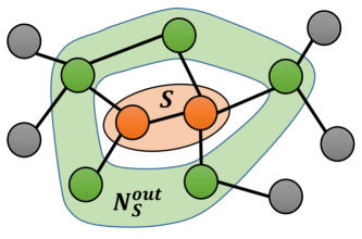
Figure 2. Neighbors of nodes in $S$

First, we “merge” all the nodes in $S$ and define a “unified neighborhood” of $S$. Specifically, let $N^{out}(u)=\{v|(u,v)\in E\}$ the set of out-neighbors of $u$ and $N^{out}_{S}=\bigcup\limits_{u\in S}N^{out}_{u}\backslash S$ the set of out-neighbors of $S$ excluding $S$. For each $v\in N^{out}_{S}$,

(10) $$P_{S,v}=1-\prod_{u\in S}(1-w(u,v)),$$

the probability that $v$ is activated directly by one (or more) node(s) in $S$. Without loss of generality, assume that $P_{S,v}\leq 1$ (otherwise, we simply add $v$ into $S$).

Assume an order on the neighborhood of $S$, that is

$$N^{out}_{S}=\{v_{1},v_{2},\dots,v_{l}\},$$

where $l=|N^{out}_{S}|$. For each $i=1..l$, let $A_{i}$ be the event that $v_{i}$ be the “first” node that gets activated directly by $S$:

$$A_{i}=\{v_{1},\ldots,v_{i-1}\ \text{are not active and }v_{i}\text{ is active after round }1\}.$$

The probability of $A_{i}$ is

(11) $$\Pr[A_{i}]=P_{S,v_{i}}\prod_{j=1}^{i-1}(1-P_{S,v_{j}}).$$

For consistency, we also denote $A_{l+1}$ the event that none of the neighbors are activated, i.e.,

(12) $$\Pr[A_{l+1}]=1-\sum_{i=1}^{l}\Pr[A_{i}].$$

Note that $A_{l+1}$ is also the event that the cascade stops right at round $0$. Such a cascade is termed a trivial cascade. As we can compute exactly the probability of trivial cascades, we do not need to sample those cascades but focus only on the non-trivial ones.

Denote by $\beta_{0}$ the probability of having at least one nodes among $v_{1},\ldots,v_{l}$ activated by $S$, i.e.,

(13) $$\beta_{0}=\sum_{i=1}^{l}\Pr[A_{i}]=1-\Pr[A_{l+1}].$$

Input: A graph $\mathcal{G}=(V,E,w)$ and a seed set $S$

Output: $Y^{(S)}$ - size of a random outward cascade from $S$

Stage 1 // Sample non-trivial neighbors of set S

Precompute $\Pr[A_{i}],i=1,\dots,l+1$ using Eq. 11 and Eq. 12

1 Select one neighbor $v_{i}$ among $v_{1},\dots,v_{l}$ with probability of selecting $v_{i}$ being $\frac{\Pr[A_{i}]}{\beta_{0}}$

2 Queue $R\leftarrow\{v_{i}\};Y^{(S)}=1$; Mark $v_{i}$ and all nodes in $S$ visited

3 for $j=i+1:l$ do

4       With a probability $P_{S,v_{j}}$ do

5             Add $v_{j}$ into $R$; $Y^{(S)}\leftarrow Y^{(S)}+1$; Mark $v_{j}$ visited.

Stage 2 // Sample from newly influenced nodes

while $R$ is non-empty do

6       $u\leftarrow R$.pop()

7       foreach unvisited neighbor $v$ of $u$ do

8             With a probability $w(u,v)$

9                  Add $v$ to $R$; $Y^{(S)}\leftarrow Y^{(S)}+1$; Mark $v$ visited.

10      

11return $Y^{(S)}$;

Algorithm 1 IICP - Importance IC Polling

We now explain the details in the Importance IC Polling Algorithm (IICP), summarized in Alg. 1. The algorithm outputs the size of the cascade minus the seed set size. We term the output of IICP the outer size of the cascade. The algorithm consists of two stages.

Stage 1. By definition, the events $A_{i},A_{2},...,A_{l},A_{l+1}$ are disjoint and form a partition of the sample space. To generate a non-trivial cascade, we first select in the first round $v_{i},i=1,\dots,l$ with a probability $\frac{\Pr[A_{i}]}{\beta_{0}},i=1,\dots,l$ (excluding $A_{l+1}$). This will guarantee that at least one of the neighbors of $S$ will be activated. Let $v_{i}$ be the selected node, after the first round $v_{i}$ becomes active and $v_{1},\ldots,v_{i-1}$ remains inactive. The nodes $v_{j}$ among $v_{i+1},\dots,v_{l}$ are then activated independently with probability $P_{S,v_{j}}$ (Eq. 10).

Stage 2. After the first stage of sampling neighbors of $S$, we get a non-trivial set of nodes directly influenced from $S$. For each of those nodes and later influenced nodes, we will sample a set of its neighbors by the naive BFS-like IC polling scheme (Kempe et al., 2003). Assume sampling neighbors of a newly influenced node $u$, each neighbor $v_{j}\in N^{out}(u)$ is influenced by $u$ with probability $w(u,v_{j})$. The neighbors of those influenced nodes are next to be sampled in the same fashion.

In addition, we keep track of the newly influenced nodes using a queue $R$ and the number of active nodes outside $S$ using $Y^{(S)}{}$.

The following lemma shows how to estimate the (expected) cascade size through the (expected) outer size of non-trivial cascades.

Lemma 4.

Given a seed set $S\subseteq V$, let $Y^{(S)}$ be the random variable associated with the output of the IICP algorithm. The following properties hold,

• $1\leq Y^{(S)}\leq n-|S|,$

• $\mathbb{I}_{out}(S)=\mathbb{E}[Y^{(S)}]\cdot\beta_{0}.$

Further, let $\Omega_{W}$ be the probability space of non-trivial cascades and $\Omega_{Y}$ the probability space for the outer size of non-trivial cascades, i.e, $Y^{(S)}{}$. The probability of $Y^{(S)}{}\in[1,n-|S|]$ is given by,

$$\Pr[Y^{(S)}{}\in\Omega_{Y}]=\sum_{W^{(S)}{}\in\Omega_{W},|W^{(S)}{}|=Y^{(S)}{}}\Pr[W^{(S)}{}\in\Omega_{W}].$$

3.2. FPRAS for Outward Influence Estimation

From Lemma 4, we can obtain an estimate $\hat{\mathbb{I}}_{out}(S)$ of $\mathbb{I}_{out}(S)$ through getting an estimate $\hat{\mathbb{E}}[Y^{(S)}{}]$ of $\mathbb{E}[Y^{(S)}{}]$ by,

$$\Pr\Big{[}(1-\epsilon)\mathbb{E}[Y^{(S)}{}]\leq\hat{\mathbb{E}}[Y^{(S)}{}]\leq(1+\epsilon)\mathbb{E}[Y^{(S)}{}]\Big{]}$$

$$=\Pr\Big{[}(1-\epsilon)\mathbb{E}[Y^{(S)}{}]\beta_{0}\leq\hat{\mathbb{E}}[Y^{(S)}{}]\beta_{0}\leq(1+\epsilon)\mathbb{E}[Y^{(S)}{}]\beta_{0}\Big{]}$$

(14) $$=\Pr\Big{[}(1-\epsilon)\mathbb{I}_{out}(S)\leq\hat{\mathbb{I}}_{out}(S)\leq(1+\epsilon)\mathbb{I}_{out}(S)\Big{]},$$

where the estimate $\hat{\mathbb{I}}_{out}(S)=\hat{\mathbb{E}}[Y^{(S)}{}]\cdot\beta_{0}$. Thus, finding an $(\epsilon,\delta)$-approximation of $\mathbb{I}_{out}(S)$ is then equivalent to finding an $(\epsilon,\delta)$-approximate $\hat{\mathbb{E}}[Y^{(S)}{}]$ of $\mathbb{E}[Y^{(S)}{}]$.

The advantage of this approach is that estimating $\mathbb{E}[Y^{(S)}{}]$, in which the random variable $Y^{(S)}{}$ has value of at least $1$, requires only a polynomial number of samples. Here the same argument on the number of samples to estimate influence spread in subsection 2.3 can be applied. Let $Y^{(S)}_{1},Y^{(S)}_{2},\dots$ be the random variables denoting the output of IICP. We can apply Lemma 3 on the set of random variables $Y^{(S)}_{1},Y^{(S)}_{2},\dots$ satisfying $1\leq Y^{(S)}_{i}\leq|V|-|S|$. Since each random variable $Y^{(S)}_{i}$ is at least 1 and hence, $\mu_{Y}=\mathbb{E}[Y^{(S)}{}]\geq 1$, we need at most a polynomial $T=O(\ln(\frac{2}{\delta})\frac{1}{\epsilon^{2}}(n-|S|))$ random variables for the Monte-Carlo estimation. Since, IICP has a worst-case time complexity $O(m+n)$, the Monte-Carlo using IICP is an FPRAS for estimating outward influence.

Theorem 3.1.

Given arbitrary $0\leq\epsilon,\delta\leq 1$ and a set $S$, the Monte-Carlo estimation using IICP returns an $(\epsilon,\delta)$-approximation of $\mathbb{I}_{out}(S)$ using $O(\ln(\frac{2}{\delta})\frac{1}{\epsilon^{2}}(n-|S|))$ samples.

In Section 5, we will show that both outward influence and influence spread can be estimated by a powerful algorithm saving a factor of more than $\frac{1}{\epsilon}$ random variables compared to this FPRAS estimation. The algorithm is built upon our mean estimation algorithms for bounded random variables proposed in the following.

4. Efficient Mean Estimation for
Bounded Random Variables

In this section, we propose an efficient mean estimation algorithm for bounded random variables. This is the core of our algorithms for accurately and efficiently estimating the outward influence and influence spread in Section 5.

We first propose an ‘intermediate’ algorithm: Generalized Stopping Rule Estimation (GSRA) which relies on a simple stopping rule and returns an $(\epsilon,\delta)$-approximate of the mean of lower-bounded random variables. The GSRA simultaneously generalizes and fixes the error of the Stopping Rule Algorithm (Dagum et al., 2000) which only aims to estimate the mean of $[0,1]$ random variables and has a technical error in its proof.

The main mean estimation algorithm, namely Robust Sampling Algorithm (RSA) presented in Alg. 3, effectively takes into account both mean and variance of the random variables. It uses GSRA as a subroutine to estimate the mean value and variance at different granularity levels.

4.1. Generalized Stopping Rule Algorithm

We aim at obtaining an $(\epsilon,\delta)$-approximate of the mean of random variables $X_{1},X_{2},\dots$. Specifically, the random variables are required to satisfy the following conditions:

• $a\leq X_{i}\leq b$, $\forall i=1,2,\dots$

• $\mathbb{E}[X_{i+1}|X_{1},X_{2},...,X_{i}]=\mu_{X},$ $\forall i=1,2,\dots$

where $0\leq a<b$ are fixed constants and (unknown) $\mu_{X}$.

Our algorithm generalizes the stopping rule estimation in (Dagum et al., 2000) that provides $(\epsilon,\delta)$ estimation of the mean of i.i.d. random variables $X_{1},X_{2},...\in[0,1]$. The notable differences are the following:

• We discover and amend an error in the stopping algorithm in (Dagum et al., 2000): the number of samples drawn by that algorithm may not be sufficient to guarantee the $(\epsilon,\delta)$-approximation.

• We allow estimating the mean of random variables that are possibly dependent and/or with different distributions. Our algorithm works as long as the random variables have the same means. In contrast, the algorithm in (Dagum et al., 2000) can only be applied for i.i.d random variables.

• Our proposed algorithm obtains an unbiased estimator of the mean, i.e. $\mathbb{E}[\hat{\mu}_{X}]=\mu_{X}$ while (Dagum et al., 2000) returns a biased one.

• Our algorithm is faster than the one in (Dagum et al., 2000) whenever the lower-bound for random variables $a>0$.

Input: Random variables $X_{1},X_{2},\dots$ and $0<\epsilon,\delta<1$

Output: An $(\epsilon,\delta)$-approximate of $\mu_{X}=E[X_{i}]$

1 If $b-a<\epsilon b$, return $\mu_{X}=a$.

2 Compute: $\epsilon^{\prime}=\epsilon\Big{(}1-\frac{\epsilon b}{(2+\frac{2}{3}\epsilon)\ln(\frac{2}{\delta})(b-a)}\Big{)};\Upsilon=(1+\epsilon)c(\epsilon^{\prime},\delta)(b-a)$;

3 Initialize $h=0,T=0$;

4 while $h<\Upsilon$ do

5       $h\leftarrow h+X_{T},T\leftarrow T+1$;

6      

return $\hat{\mu}_{X}=h/T$;

Algorithm 2 Generalized Stopping Rule Alg. (GSRA)

Our Generalized Stopping Rule Algorithm (GSRA) is described in details in Alg. 2. Denote $c(\epsilon,\delta)=(2+\frac{2}{3}\epsilon)\ln(\frac{2}{\delta})\frac{1}{\epsilon^{2}}$.

The algorithm contains two main steps: 1) Compute the stopping threshold $\Upsilon$ (Line 2) which relies on the value of $\epsilon^{\prime}$ computed from the given precision parameters $\epsilon,\delta$ and the range $[a,b]$ of the random variables; 2) Consecutively acquire the random variables until the sum of their outcomes exceeds $\Upsilon$ (Line 4-5). Finally, it returns the average of the outcomes, $\hat{\mu}_{X}=h/T$ (Line 6), as an estimate for the mean, $\mu_{X}$. Notice that $\Upsilon$ in GSRA depends on $(b-a)$ and thus, getting tighter bounds on the range of random variables holds a key for the efficiency of GSRA in application perspectives.

The approximation guarantee and number of necessary samples are stated in the following theorem.

Theorem 4.1.

The Generalized Stopping Rule Algorithm (GSRA) returns an $(\epsilon,\delta)$-approximate $\hat{\mu}_{X}$ of $\mu_{X}$, i.e.,

(15) $$\Pr[(1-\epsilon)\mu_{X}\leq\hat{\mu}_{X}\leq(1+\epsilon)\mu_{X}]>1-\delta,$$

and, the number of samples $T$ satisfies,

(16) $$\Pr[T\leq(1+\epsilon)\Upsilon/\mu_{X}]>1-\delta/2.$$

The hole in the Stopping Rule Algorithm in (Dagum et al., 2000). The estimation algorithm in (Dagum et al., 2000) for estimating the mean of random variables in range $[0,1]$ also bases on a main stopping rule condition as our GSRA. It computes a threshold

(17) $$\Upsilon_{1}=1+(1+\epsilon)4(e-2)\ln(\frac{2}{\delta})\frac{1}{\epsilon^{2}},$$

where $e$ is the base of natural logarithm, and generates samples $X_{j}$ until $\sum_{j=1}^{T}X_{j}\geq\Upsilon_{1}$. The algorithm returns $\hat{\mu}_{X}=\frac{\Upsilon_{1}}{T}$ as a biased estimate of $\mu_{X}$.

Unfortunately, the threshold $\Upsilon_{1}$ to determine the stopping time does not completely account for the fact that the necessary number of samples should go over the expected one in order to provide high solution guarantees. This actually causes a flaw in their later proof of the correctness.

To amend the algorithm, we slightly strengthen the stopping condition by replacing the $\epsilon$ in the formula of $\Upsilon$ with an $\epsilon^{\prime}=\epsilon\Big{(}1-\frac{\epsilon b}{(2+\frac{2}{3}\epsilon)\ln(\frac{2}{\delta})(b-a)}\Big{)}$ (Line 2, Alg. 2). Since $\epsilon b<b-a$ (else the algorithm returns $\mu_{X}=a$) and assume w.l.o.g. that $\delta<1/2$, it follows that $\epsilon^{\prime}\geq 0.729\epsilon$. Thus the number of samples, in comparison to those in the stopping rule algorithm in (Dagum et al., 2000) increases by at most a constant factor.

Benefit of considering the lower-bound $a$. By dividing the random variables by $b$, one can apply the stopping rule algorithm in (Dagum et al., 2000) on the normalized random variables. The corresponding value of $\Upsilon$ is then

(18) $$\Upsilon=1+(1+\epsilon)(2+\frac{2}{3}\epsilon)\ln(\frac{2}{\delta})\frac{1}{\epsilon^{\prime 2}}b$$

$\Upsilon$ in our proposed algorithm is however smaller by a multiplicative factor of $\frac{b-a}{b}$. Thus it is faster than the algorithm in (Dagum et al., 2000) by a factor of $\frac{b-a}{b}$ on average. Note that in case of estimating the influence, we have $a=1,b=n-|S|$. Compared to algorithm applied (Dagum et al., 2000) directly, our GSRA algorithm saves the generated samples by a factor of $\frac{b-a}{b}=\frac{n-|S|-1}{n}=1-\frac{|S|+1}{n}<1$.

Martingale theory to cope with weakly-dependent random variables. To prove Theorem 4.1, we need a stronger Chernoff-like bound to deal with the general random variables $X_{1},X_{2},\dots$ in range $[a,b]$ presented in the following.

Let define random variables $Y_{i}=\sum_{j=1}^{i}(X_{j}-\mu_{X}),\forall i\geq 1$. Hence, the random variables $Y_{1},Y_{2},\dots$ form a Martingale (Mitzenmacher and Upfal, 2005) due to the following,

$$\mathbb{E}[Y_{i}|Y_{1},\dots,Y_{i-1}]=\mathbb{E}[Y_{i-1}]+\mathbb{E}[X_{i}-\mu_{X}]=\mathbb{E}[Y_{i-1}].$$

Then, we can apply the following lemma from (Chung and Lu, 2006) stating,

Lemma 5.

Let $Y_{1},\dots,Y_{i},...$ be a martingale, such that $|Y_{1}|\leq\alpha$, $|Y_{j}-Y_{j-1}|\leq\alpha$ for all $j=[2,i]$, and

(19) $$\mathrm{Var}[Y_{1}]+\sum_{j=2}^{i}\mathrm{Var}[Y_{j}|Y_{1},\dots,Y_{j-1}]\leq\beta.$$

Then, for any $\lambda\geq 0$,

(20) $$\Pr[Y_{i}-\mathbb{E}[Y_{i}]\geq\lambda]\leq\exp(-\frac{\lambda^{2}}{2/3\cdot\alpha\cdot\lambda+2\cdot\beta})$$

In our case, we have $|Y_{1}|=|X_{1}-\mu_{X}|\leq b-a$, $|Y_{j}-Y_{j-1}|=|X_{i}-\mu_{X}|\leq b-a$, $\mathrm{Var}[Y_{1}]=\mathrm{Var}[X_{1}-\mu_{X}]=\mathrm{Var}[X]$ and $\mathrm{Var}[Y_{j}|Y_{1},\dots,Y_{j}]=\mathrm{Var}[X_{j}-\mu_{X}]=\mathrm{Var}[X]$. Apply Lemma 2 with $i=T$ and $\lambda=\epsilon T\mu_{X}$, we have,

(21) $$\Pr\Big{[}\sum_{j=1}^{T}X_{j}\geq(1+\epsilon)\mu_{X}T\Big{]}\leq\exp\big{(}\frac{-\epsilon^{2}T^{2}\mu^{2}_{X}}{\frac{2}{3}(b-a)\epsilon\mu_{X}T+2\mathrm{Var}[X]T}\big{)}$$

Then, since $\mathrm{Var}[X]\leq\mu_{X}(b-\mu_{X})\leq\mu_{X}(b-a)$ ( since Bernoulli random variables with the same mean $\mu_{X}$ have the maximum variance), we also obtain,

(22) $$\Pr\Big{[}\sum_{j=1}^{T}X_{j}\geq(1+\epsilon)\mu_{X}T\Big{]}\leq\exp\big{(}\frac{-\epsilon^{2}T\mu_{X}}{(2+\frac{2}{3}\epsilon)(b-a)}\big{)}.$$

Similarly, $-Y_{1},\dots,-Y_{i},\dots$ also form a Martingale and applying Lemma 5 gives the following probabilistic inequality,

(23) $$\Pr\Big{[}\sum_{j=1}^{T}X_{j}\leq(1-\epsilon)\mu_{X}T\Big{]}\leq\exp\big{(}-\frac{\epsilon^{2}T\mu_{X}}{2(b-a)}\big{)}.$$

Input: Two streams of i.i.d. random variables, $X_{1},X_{2},\dots$ and $X^{\prime}_{1},X^{\prime}_{2},\dots$ and $0<\epsilon,\delta<1$

Output: An $(\epsilon,\delta)$-approximate $\hat{\mu}_{X}$ of $\mu_{X}$

Step 1 // Obtain a rough estimate $\hat{\mu}^{\prime}_{X}$ of $\mu_{X}$

if $\epsilon\geq 1/4$ then

1       return $\hat{\mu}_{X}\leftarrow$ GSRA($<X_{1},X_{2},\ldots>,\epsilon,\delta$)

2      

3$\hat{\mu}^{\prime}_{X}\leftarrow$ GSRA($<X_{1},X_{2},\ldots>,\sqrt{\epsilon},\delta/3$)

Step 2 // Estimate the variance $\hat{\sigma}^{2}_{X}$

$\Upsilon_{2}=2\frac{1+\sqrt{\epsilon}}{1-\sqrt{\epsilon}}(1+\ln(\frac{3}{2})/\ln(\frac{2}{\delta}))\cdot\Upsilon;N_{\sigma}=\Upsilon_{2}\cdot\epsilon/\hat{\mu}^{\prime}_{X};\Delta=0$;

  // $\Upsilon$ is defined the same as in Alg. 2

for $i=1:N_{\sigma}$ do

4       $\Delta\leftarrow\Delta+(X^{\prime}_{2i}-X^{\prime}_{2i+1})^{2}$/2;

5      

6$\hat{\rho}_{X}=\max\{\hat{\sigma}_{X}^{2}=\Delta/N_{\sigma},\epsilon\hat{\mu}^{\prime}_{X}(b-a)\}$;

Step 3 // Estimate $\mu_{X}$

Set $T=\Upsilon_{2}\cdot\hat{\rho}_{X}/(\hat{\mu}^{\prime 2}_{X}(b-a)),S\leftarrow 0$;

7 for $i=1:T$ do

8       $S\leftarrow S+X_{i}$;

9return $\hat{\mu}_{X}=S/T$;

Algorithm 3 Robust Sampling Algorithm (RSA)

4.2. Robust Sampling Algorithm

Our previously proposed GSRA algorithm may have problem in estimating means of random variables with small variances. An important tool that we rely on to prove the approximation guarantee in GSRA is the Chernoff-like bound in Eq. 22 and Eq. 23. However, from the inequality in Eq. 21, we can also derive the following stronger inequality,

$$\Pr\Big{[}\sum_{j=1}^{T}X_{j}\geq(1+\epsilon)\mu_{X}T\Big{]}\leq\exp\Big{(}\frac{-\epsilon^{2}T^{2}\mu^{2}_{X}}{\frac{2}{3}(b-a)\epsilon\mu_{X}T+2\mathrm{Var}[X]T}\Big{)}$$

(24) $$\qquad\text{ }\leq\exp\Big{(}\frac{-\epsilon^{2}T\mu^{2}_{X}}{(2+\frac{2}{3})\max\{\epsilon\mu_{X}(b-a),\mathrm{Var}[X]\}}\Big{)}.$$

In many cases, random variables have small variances and hence $\max\{\epsilon\mu_{X}(b-a),\mathrm{Var}[X]\}=\epsilon\mu_{X}(b-a)$. Thus, Eq. 24 is much stronger than Eq. 22 and can save a factor of $\frac{1}{\epsilon}$ in terms of required observed influences translating into the sample requirement. However, both the mean and variance are not available.

To achieve a robust sampling algorithm in terms of sample complexity, we adopt and improve the $\mathcal{AA}$ algorithm in (Dagum et al., 2000) for general cases of $[a,b]$ random variables. The robust sampling algorithms (RSA) subsequently will estimate both the mean and variance in three steps: 1) roughly estimate the mean value with larger error ($\sqrt{\epsilon}$ or a constant); 2) use the estimated mean value to compute the number of samples necessary for estimating the variance; 3) use both the estimated mean and variance to refine the required samples to estimate mean value with desired error ($\epsilon,\delta$).

Let $X_{1},X_{2},\dots$ and $X^{\prime}_{1},X^{\prime}_{2},\dots$ are two streams of i.i.d random variables. Our robust sampling algorithm (RSA) is described in Alg. 3. It consists of three main steps:

• If $\epsilon\geq 1/4$, run GSRA with parameter $\epsilon,\delta$ and return the result (Line 1-2). Otherwise, assume $\epsilon<1/4$ and use the Generalized Stopping Rule Algorithm (Alg. 2) to obtain an rough estimate $\hat{\mu}^{\prime}_{X}$ using parameters of $\epsilon^{\prime}=\sqrt{\epsilon}<1/2,\delta^{\prime}=\delta/3$ (Line 3).

• Use the estimated $\hat{\mu}^{\prime}_{X}$ in step 1 to compute the necessary number of samples, $N_{\sigma}$, to estimate the variance of $X_{i}$, $\hat{\sigma}_{X}^{2}$. Note that this estimation uses the second set of samples, $X^{\prime}_{1},X^{\prime}_{2},\dots$

• Use both $\hat{\mu}^{\prime}_{X}$ in step 1 and $\hat{\sigma}_{X}^{2}$ in step 2 to compute the actual necessary number of samples, $T$, to approximate the mean $\mu_{X}$. Note that this uses the same set of samples $X_{1},X_{2},\dots$ as in the first step.

The numbers of samples used in the first two steps are always less than a constant times $\Upsilon\cdot\epsilon/\mu_{X}$ which is the minimum samples that we can achieve using the variance. This is because the first takes the error parameter $\sqrt{\epsilon}$ which is higher than $\epsilon$ and the second step uses $N_{\sigma}=\Upsilon_{2}\cdot\epsilon/\hat{\mu}^{\prime}_{X}$ samples.

At the end, the algorithm returns the influence estimate $\hat{\mu}_{X}$ which is the average over $T$ samples, $\hat{\mu}_{X}=S/T$. The estimation guarantees are stated in the following theorem.

Theorem 4.2.

Let $X$ be the probability distribution that $X_{1},X_{2},\dots$ and $X^{\prime}_{1},X^{\prime}_{2},\dots$ are drawn from. Let $\hat{\mu}_{X}$ be the estimate of $\mathbb{E}[X]$ returned by Alg. 3 and $T$ be the number of drawn samples in Alg. 3 w.r.t. $\epsilon,\delta$. We have,

• $\Pr[\mu_{X}(1-\epsilon)\leq\hat{\mu}_{X}\leq(1+\epsilon)\mu_{X}]\geq 1-\delta$,

• There is a universal constant $c^{\prime}$ such that

  (25) $$\Pr[T>c^{\prime}\Upsilon\rho_{X}/(\mu^{2}_{X}(b-a))]\leq\delta$$

  where $\rho_{Z}=\max\{\epsilon\mu_{X}(b-a),\mathrm{Var}[X]\}$.

Compared to the $\mathcal{AA}$ algorithm in (Dagum et al., 2000), first of all, we replace their stopping rule algorithm with GSRA and also, we change the computation of $\Upsilon_{2}$ which is always smaller than that of (Dagum et al., 2000) by a factor of $1+\sqrt{\epsilon}-2\epsilon\geq 1$ when $\epsilon\leq 1/4$.

5. Influence Estimation at Scale

This section applies our RSA algorithm to estimate both the outward influence and the traditional influence spread.

5.1. Outward Influence Estimation

We directly apply RSA algorithm on two streams of i.i.d. random variables $Y^{(S)}_{1},Y^{(S)}_{2},\dots$ and $Y^{\prime(S)}_{1},Y^{\prime(S)}_{2},\dots$, which are generated by IICP sampling algorithm, with the precision parameters $\epsilon,\delta$.

The algorithm is called Scalable Outward Influence Estimation Algorithm (SOIEA) and presented in Alg. 4 which generates two streams of random variables $Y^{(S)}_{1},Y^{(S)}_{2},\dots$ and $Y^{\prime(S)}_{1},Y^{\prime(S)}_{2},\dots$ (Line 1) and applies RSA algorithm on these two streams (Line 2). Note that outward influence estimate is achieved by scaling down $\mu_{Y}$ by $\beta_{0}$ (Lemma 4).

Input: A probabilistic graph $\mathcal{G}$, a set $S$ and $\epsilon,\delta$

Output: $\hat{\mathbb{I}}(S)$ - an $(\epsilon,\delta)$-estimate of $\mathbb{I}(S)$

1 Generate two streams of i.i.d. random variables $Y^{(S)}_{1},Y^{(S)}_{2},\dots$ and $Y^{\prime(S)}_{1},Y^{\prime(S)}_{2},\dots$ by IICP algorithm.

return $\hat{\mathbb{I}}_{out}(S)\leftarrow\beta_{0}\cdot\textsf{RSA}(<Y^{(S)}_{1},\dots>,<Y^{\prime(S)}_{1},\dots>,\epsilon,\delta)$

Algorithm 4 SOIEA Alg. to estimate outward influence

We obtain the following theoretical results incorporated from Theorem 4.2 of RSA and IICP samples.

Theorem 5.1.

The SOIEA algorithm gives an $(\epsilon,\delta)$ outward influence estimation. The observed outward influences (sum of $Y^{(S)}{}$) and the number of generated random variables are in $O(\ln(\frac{2}{\delta})\frac{1}{\epsilon^{2}}\frac{\rho_{Y}}{\mathbb{I}_{out}(S)/\beta_{0}})$ and $O(\ln(\frac{2}{\delta})\frac{1}{\epsilon^{2}}\frac{\rho_{Y}}{\mathbb{I}_{out}^{2}(S)/\beta_{0}^{2}})$ respectively, where $\rho_{Y}=\max\{\epsilon\mathbb{I}_{out}(S)(n-|S|-1)/\beta_{0},\mathrm{Var}[Y^{(S)}_{i}]\}$.

Note that $\mathbb{E}[Y^{(S)}{}]=\mathbb{I}_{out}(S)/\beta_{0}\geq 1$.

5.2. Influence Spread Estimation

Not only is the concept of outward influence helpful in discriminating the relative influence of nodes but also its sampling technique, IICP, can help scale up the estimation of influence spread (IE) to billion-scale networks.

Naive approach. A naive approach is to 1) obtain an $(\epsilon,\delta)$-approximation $\hat{\mathbb{I}}_{out}(S)$ of $\mathbb{I}_{out}(S)$ using Monte-Carlo estimation 2) return $\hat{\mathbb{I}}_{out}(S)+|S|$. It is easy to show that this approach return an $(\epsilon,\delta)$-approximation for $\mathbb{I}(S)$. This approach will require $O(\ln(\frac{2}{\delta})\frac{1}{\epsilon^{2}}n)$ IICP random samples.

However, the naive approach is not optimized to estimate influence due to several reasons: 1) a loose bound $\mu_{Y}=\mathbb{E}[Y^{(S)}{}]\geq 1$ is applied to estimate outward influence; 2) casting from $(\epsilon,\delta)$-approximation of outward influence to $(\epsilon,\delta)$-approximation of influence introduces a gap that can be used to improve the estimation guarantees. We next propose more efficient algorithms based on Importance IC Sampling to achieve an $(\epsilon,\delta)$-approximate of both outward influence and influence spread. Our methods are based on two effective mean estimation algorithms.

Our approach. Based on the observations that

• $1\leq Y^{(S)}\leq n-|S|$, i.e., we know better bounds for $Y^{(S)}$ in comparison to the cascade size which is in the range $[1,n]$.

• As we want to have an $(\epsilon,\delta)$-approximation for $Y^{(S)}+|S|$, the fixed add-on $|S|$ can be leveraged to reduce the number of samples.

We combine the effective RSA algorithm with our Importance IC Polling (IICP) for estimating the influence spread of a set $S$. For influence spread estimation, we will analyze random variables based on samples generated by our Importance IC Polling scheme and use those to devise an influence estimation algorithm.

Since outward influence and influence spread differ by an additive factor of $|S|$, for each outward sample $Y^{(S)}{}$ generated by IICP, let define a corresponding variable $Z^{(S)}{}$,

(26) $$Z^{(S)}{}=Y^{(S)}{}\cdot\beta_{0}+|S|,$$

where $\beta_{0}$ is defined in Eq. 13. We obtain,

• $|S|+\beta_{0}\leq Z^{(S)}{}\leq|S|+\beta_{0}(n-|S|)$,

• $\mathbb{E}[Z^{(S)}{}]=\mathbb{E}[Y^{(S)}{}]\cdot\beta_{0}+|S|=\mathbb{I}_{out}(S)+|S|=\mathbb{I}(S)$,

and thus we can to approximate $\mathbb{I}(S)$ by estimating $\mathbb{E}[Z^{(S)}{}]$.

Recall that to estimate the influence $\mathbb{I}(S)$ of a seed set $S$, all the previous works (Kempe et al., 2003; Leskovec et al., 2007; Chen et al., 2010) resort to simulating many influence cascades from $S$ and take the average size of those generated cascades. Let call $M^{(S)}{}$ the random variable representing the size of such a influence cascade. Then, we have $\mathbb{E}[M^{(S)}{}]=\mathbb{I}(S)$. Although both $Z^{(S)}{}$ and $M^{(S)}{}$ can be used to estimate the influence, they have different variances that lead to difference in convergence speed when estimating their means. The relation between variances of $Z^{(S)}{}$ and $M^{(S)}{}$ is stated as follows.

Lemma 6.

Let $Z^{(S)}{}$ defined in Eq. 26 and $M^{(S)}{}$ be random variable for the size of a influence cascade, the variances of $Z^{(S)}{}$ and $M^{(S)}{}$ satisfy,

(27) $$\mathrm{Var}[Z^{(S)}{}]=\beta_{0}\cdot\mathrm{Var}[M^{(S)}]-(1-\beta_{0})\mathbb{I}_{out}^{2}(S)$$

Note that $0\leq\beta_{0}\leq 1$ and $\mathbb{I}(S)\geq|S|$. Thus, the variance of $Z^{(S)}{}$ is much smaller than $M^{(S)}{}$. Our proposed RSA on random variables $X_{i}$ makes use of the variances of random variables and thus, benefits from the small variance of $Z^{(S)}{}$ compared to the same algorithm on the previously known random variables $M^{(S)}{}$.

Input: A probabilistic graph $\mathcal{G}$, a set $S$ and $\epsilon,\delta$

Output: $\hat{\mathbb{I}}(S)$ - an $(\epsilon,\delta)$-estimate of $\mathbb{I}(S)$

1 Generate two streams of i.i.d. random variables $Y^{(S)}_{1},Y^{(S)}_{2},\dots$ and $Y^{\prime(S)}_{1},Y^{\prime(S)}_{2},\dots$ by IICP algorithm.

2 Compose two streams $Z^{(S)}_{1},Z^{(S)}_{2},\dots$ and $Z^{\prime(S)}_{1},Z^{\prime(S)}_{2},\dots$ from $Y^{(S)}_{1},Y^{(S)}_{2},\dots$ and $Y^{\prime(S)}_{1},Y^{\prime(S)}_{2},\dots$ using Eq. 26.

return $\hat{\mathbb{I}}(S)\leftarrow$RSA($<Z^{(S)}_{1},\dots>,<Z^{\prime(S)}_{1},\dots>,\epsilon,\delta$)

Algorithm 5 SIEA Alg. to estimate influence spread

Thus, we apply the RSA on random variables generated by IICP to develop Scalable Influence Estimation Algorithm (SIEA). SIEA is described in Alg. 5 which consists of two main steps: 1) generate i.i.d. random variables by IICP and 2) convert those variables to be used in RSA to estimate influence of $S$. The results are stated as follows,

Theorem 5.2.

The SIEA algorithm gives an $(\epsilon,\delta)$ influence spread estimation. The observed influences (sum of random variables $Z^{(S)}{}$) and the number of generated random variables are in $O(\ln(\frac{2}{\delta})\frac{1}{\epsilon^{2}}\frac{\rho_{Z}}{\mathbb{I}(S)})$ and $O(\ln(\frac{2}{\delta})\frac{1}{\epsilon^{2}}\frac{\rho_{Z}}{\mathbb{I}^{2}(S)})$, where $\rho_{Z}=\max\{\epsilon\mathbb{I}(S)\beta_{0}(n-|S|-1),\mathrm{Var}[Z^{(S)}_{i}]\}$.

Comparison to INFEST (Lucier et al., 2015). Compared to the most recent state-of-the-art influence estimation in (Lucier et al., 2015) that requires $O(\frac{n\log^{5}(n)}{\epsilon^{2}})$ observed influences, the SIEA algorithm incorporating IICP sampling with RSA saves at least a factor of $\log^{4}(n)$. That is because the necessary observed influences in SIEA is bounded by $O(\ln(\frac{2}{\delta})\frac{1}{\epsilon^{2}}\frac{\beta_{0}\rho_{Z}}{\mathbb{I}(S)})$. Since $\mathrm{Var}[Z^{(S)}_{i}]\leq\mathbb{I}(S)(|S|+\beta_{0}(n-|S|)-\mathbb{I}(S))\leq\mathbb{I}(S)(n-|S|-1)$ and hence, $\rho_{Z}\leq\mathbb{I}(S)(n-|S|-1)$, when $\delta=\frac{1}{n}$ as in (Lucier et al., 2015), the observed influences is then,

(28) $$O(\ln(\frac{2}{\delta})\frac{1}{\epsilon^{2}}\frac{\rho_{Z}}{\mathbb{I}(S)})\leq O(\frac{n\log(2/\delta)}{\epsilon^{2}})\leq O(\frac{n\log(n)}{\epsilon^{2}})$$

Consider $\epsilon,\delta$ as constants, the observed influences is $O(n)$.

5.3. Influence Spread under other Models

We can easily apply the RSA estimation algorithm to obtain an $(\epsilon,\delta)$-estimate of the influence spread under other cascade models as long as there is a Monte-Carlo sampling procedure to generate sizes of random cascades. For most stochastic diffusion models, including both discrete-time models, e.g. the popular LT with a naive sample generator described in (Kempe et al., 2003), SI and SIR (Daley et al., 2001) or their variants with deadlines (Nguyen et al., 2016), and continuous-time models (Du et al., 2013), designing such a Monte-Carlo sampling procedure is straightforward. Since the influence cascade sizes are at least the seed size, we always needs at most $O(n)$ samples.

To obtain more efficient sampling procedures, we can extend the idea of sampling non-trivial cascade in IICP to other models. Such sampling procedures in general will result in random variables with smaller variances and tighter bounds on the ranges. In turns, RSA, that benefits from smaller variance and range, will requires fewer samples for estimation.

5.4. Parallel Estimation Algorithms

We develop the parallel versions of our algorithms to speed up the computation and demonstrate the easy-to-parallelize property of our methods. Our main idea is that the random variable generation by IICP can be run in parallel. In particular, random variables used in each step of the core RSA algorithm can be generated simultaneously. Recall that IICP only needs to store a queue of newly active nodes, an array to mark the active nodes and a single variable $Y^{(S)}$. In total, each thread requires space in order of the number of active nodes in that simulation, $O(Y^{(S)})$, which is at most linear with size of the graph $O(n)$. In fact due to the stopping condition of linear number of observed influences, the total size of all the threads is bounded by $O(n)$ assumed the number of threads is relatively small compared to $n$.

Moreover, our algorithms can be implemented efficiently in terms of communication cost in distributed environments. This is because the output of IICP algorithm is just a single number $Y^{(S)}$ and thus, worker nodes in a distributed environment only communicate that single number back to the node running the estimation task. Here each IICP node holds a copy of the graph. However, the programming model needs to be considered carefully. For instance, as pointed out in many studies that the famous MapReduce is not a good fit for iterative graph processing algorithms (Gupta et al., 2013; Lin and Schatz, 2010).

6. Experiments

We will experimentally show that Outward Influence Estimation (SOIEA) and Outward-Based Influence Estimation (SIEA) are not only several orders of magnitudes faster than existing state-of-the-art methods but also consistently return much smaller errors. We present empirical validation of our methods on both real world and synthetic networks.

6.1. Experimental Settings

Algorithms. We compare performance of SOIEA and SIEA with the following algorithms:

• INFEST (Lucier et al., 2015): A recent influence estimation algorithm by Lucier et al. (Lucier et al., 2015) in KDD’15 that provides approximation guarantees. We reimplement the algorithm in C++ accordingly to the description in (Lucier et al., 2015).

• MC${}_{\text{10K}}$, MC${}_{\text{100K}}$: Variants of Monte-Carlo method that generates the traditional influence cascades (Kempe et al., 2003; Leskovec et al., 2007) to estimate (outward) influence spread.

• MC_ϵ,δ: The Monte-Carlo method that uses the traditional influence cascades and guarantees $(\epsilon,\delta)$-estimation. Following (Lucier et al., 2015), MC_ϵ,δ is only for measuring the running time of the normal Monte-Carlo to provide the same $(\epsilon,\delta)$-approximation guarantee. In particular, we obtain running time of MC_ϵ,δ by interpolating from that from MC${}_{\text{10K}}$, i.e. $\frac{1}{\epsilon^{2}}\ln(\frac{1}{\delta})n\frac{\textsf{Time}(\text{{MC${}_{\text{10K}}$}{}})}{10000}$.

Table 2. Datasets’ Statistics

Dataset	#Nodes	#Edges	Avg. Degree
NetHEP	15K	59K	4.1
NetPHY	37K	181K	13.4
Epinions	75K	841K	13.4
DBLP	655K	2M	6.1
Orkut	3M	117M	78.0
Twitter (Kwak et al., 2010)	41.7M	1.5G	70.5
Friendster	65.6M	1.8G	54.8
From http://snap.stanford.edu

Table 3. Comparing performance of algorithms in estimating outward influences

		Avg. Rel. Error (%)				Max. Rel. Error (%)				Running time (sec)
Dataset	Edge Models	SOIEA	MC${}_{\text{10K}}$	MC${}_{\text{100K}}$		SOIEA	MC${}_{\text{10K}}$	MC${}_{\text{100K}}$		SOIEA	MC${}_{\text{10K}}$	MC${}_{\text{100K}}$	MCϵ,δ
NetHEP	$wc$	0.3	1.9	0.6		2.3	25.0	8.9		0.1	0.1	0.1	12.3
	$p=0.1$	1.0	3.7	1.2		9.7	63.0	17.2		0.2	0.1	1.0	149.5
	$p=0.01$	0.0	4.5	1.6		0.2	20.2	9.2		0.2	0.1	0.1	8.8
	$p=0.001$	0.0	19.2	4.6		0.1	100.0	26.4		0.2	0.1	0.1	8.5
NetPHY	$wc$	0.1	1.4	0.4		1.5	32.8	6.2		0.4	0.1	0.1	34.7
	$p=0.1$	0.5	4.0	1.3		6.6	46.3	18.5		0.5	0.1	0.5	203.0
	$p=0.01$	0.0	5.5	1.7		0.2	30.4	10.7		0.6	0.1	0.1	25.0
	$p=0.001$	0.0	19.1	5.1		0.0	80.0	28.1		0.7	0.1	0.1	24.0

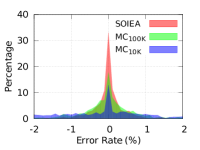
(a) WC model

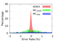
(b) $p=0.1$

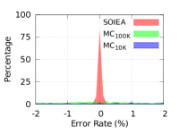
(c) $p=0.01$

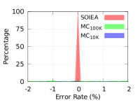
(d) $p=0.001$

Figure 3. Error distributions (histogram) of the approximation errors of SOIEA, MC${}_{\text{10K}}$, MC${}_{\text{100K}}$ on NetHEP

Datasets. We use both real-world networks and synthetic networks generated by GTgraph (Bader and Madduri, 2006). For real world networks, we choose a set of 7 datasets with sizes from tens of thousands to 65.6 millions. Table 2 gives a summary. GTgraph generates synthetic graphs with varying number of nodes and edges.

Metrics. We compare the performance of the algorithms in terms of solution quality and running time. To compare the solution quality, we adopt the relative error which shows how far the estimated number from the “ground truth”. The relative error of outward influence is computed as follows:

(29) $$|\frac{\hat{\mathbb{I}}_{out}(S)}{\mathbb{I}_{out}(S)}-1|\cdot 100\%$$

where $\hat{\mathbb{I}}_{out}(S)$ is estimated outward influence of seed set $S$ by the algorithm, $\mathbb{I}_{out}(S)$ is “ground truth” for $S$.

Similarly, relative error of influence spread is,

(30) $$|\frac{\hat{\mathbb{I}}(S)}{\mathbb{I}(S)}-1|\cdot 100\%$$

We test the algorithms on estimating different seed set sizes. For each size, we generate a set of 1000 random seed sets. We will report the average relative error (Avg. Rel. Error) and maximum relative error (Max. Rel. Error).

Ground-truth computation. We use estimates of influence and outward influence with a very small error corresponding to the setting $\epsilon=0.005,\delta=1/n$. We note that previous researches (Lucier et al., 2015; Tang et al., 2015) compute the “ground truth” by running Monte-Carlo with 10,000 samples which is not sufficient as we will show later in our experiments.

Parameter Settings. For each of the datasets, we consider two common edge weighting models:

• Weighted Cascade (WC): The weight of edge $(u,v)$ is calculated as $w(u,v)=\frac{1}{d_{in}(v)}$ where $d_{in}(v)$ denotes the in-degree of node $v$, as in (Chen et al., 2010; Tang et al., 2014; Cohen et al., 2014; Tang et al., 2015; Nguyen et al., 2016b).

• Constant model: All the edges has the same constant probability $p$ as in (Kempe et al., 2003; Chen et al., 2010; Cohen et al., 2014). We consider three different values of $p$, i.e. $0.1,0.01,0.001$.

We set $\epsilon=0.1$, $\delta=1/n$ for SOIEA and SIEA by default or explicitly stated otherwise.

Environment. All algorithms are implemented in C++ and compiled using GCC 4.8.5. We conduct all experiments on a CentOS 7 workstation with two Intel Xeon 2.30GHz CPUs adding up to 20 physical cores and 250GB RAM.

6.2. Outward Influence Estimation

We compare SOIEA against MC${}_{\text{10K}}$ and MC${}_{\text{100K}}$ in four different edge models on NetHEP and NetPHY dataset. The results are presented in Table 3 and Figure 3.

6.2.1. Solution Quality

Table 3 illustrates that the outward influences computed by SOIEA consistently have much smaller errors in both average and maximum cases than MC${}_{\text{10K}}$ and MC${}_{\text{100K}}$ in all edge models. In particular, on NetHEP with $p=0.001$ edge model, SOIEA has average relative error close to 0% while it is 19.2% and 4.6% for MC${}_{\text{10K}}$, MC${}_{\text{100K}}$ respectively; the maximum relative errors of MC${}_{\text{10K}}$, MC${}_{\text{100K}}$ in this case are 100%, 26.4% which are much higher than SOIEA of 0.1%. Apparently, MC${}_{\text{100K}}$ has smaller error rate than MC${}_{\text{10K}}$ since it uses 10 times more samples.

Figure 3 shows error distributions of SOIEA, MC${}_{\text{10K}}$, and MC${}_{\text{100K}}$ on NetHEP. In all considered edge models, SOIEA’s error highly concentrates around 0% while errors of MC${}_{\text{10K}}$ and MC${}_{\text{100K}}$ wildly spread out to a very large spectrum. In particular, SOIEA has a huge spike at the 0 error while both MC${}_{\text{10K}}$ and MC${}_{\text{100K}}$ contain two heavy tails in two sides of their error distributions. Moreover, when $p$ gets smaller, the tails get larger as more and more empty influence simulations are generated in the traditional method.

6.2.2. Running Time

From Table 3, the running time of MC${}_{\text{10K}}$ and MC${}_{\text{100K}}$ is close to that of SOIEA while MC_ϵ,δ takes up to 700 times slower than the others. Thus, in order to achieve the same approximation guarantee as SOIEA, the naive Monte-Carlo will need 700 more time than SOIEA.

Overall, SOIEA achieves significantly better solution quality and runs substantially faster than Monte-Carlo method. With larger number of samples, Monte-Carlo method can improve the quality but the running time severely suffers.

6.3. Influence Spread Estimation

This experiment evaluates SIEA by comparing its performance with the most recent state-of-the-art INFEST and naive Monte-Carlo influence estimation. Here, we use WC model to assign probabilities for the edges. We set the $\epsilon$ parameter for INFEST to 0.4 since we cannot run with smaller value of $\epsilon$ for this algorithm. Note that INFEST guarantees an error of $(1+8\epsilon)$, which is equivalent to a maximum relative error of 320%. For a fair comparison, we also run SIEA with $\epsilon=0.4$. We use the gold-standard 10000 samples for the Monte-Carlo method (MC${}_{\text{10K}}$). We set a time limit of 6 hours for all algorithms.

Table 4. Comparing performance of algorithms in estimating influence spread in WC Model (seed set size $|S|=1$)

	Avg. Rel. Error (%)				Max. Rel. Error (%)				Running time (sec.)
Dataset	SIEA	MC${}_{\text{10K}}$	INFEST		SIEA	MC${}_{\text{10K}}$	INFEST		SIEA	SIEA (16 cores)	MC${}_{\text{10K}}$	MCϵ,δ	INFEST
NetHEP	0.2	1.2	17.7		1.5	6.6	82.7		0.1	0.1	0.0	0.8	3417.6
NetPHY	0.1	0.4	22.9		0.6	5.3	43.0		0.1	0.1	0.0	2.6	8517.7
Epinions	0.9	5.3	n/a		5.2	19.7	n/a		0.2	0.1	0.0	21.9	n/a
DBLP	0.3	1.2	n/a		1.9	8.7	n/a		2.8	1.3	0.1	770.4	n/a
Orkut	0.5	3.0	n/a		3.2	16.0	n/a		54.2	4.76	2.9	$8.2\cdot 10^{4}$	n/a
Twitter	1.0	37.1	n/a		3.1	240.8	n/a		1272.3	106.2	7.9	$3.5\cdot 10^{6}$	n/a
Friendster	0.1	3.1	n/a		0.6	23.6	n/a		1510.1	165.1	2.8	$2.1\cdot 10^{6}$	n/a

Table 5. Comparing performance of algorithms in estimating influence spread in WC Model (seed set size $|S|=5\%|V|$)

	Avg. Rel. Error (%)				Max. Rel. Error (%)				Running time (sec.)
Dataset	SIEA	MC${}_{\text{10K}}$	INFEST		SIEA	MC${}_{\text{10K}}$	INFEST		SIEA	SIEA (16 cores)	MC${}_{\text{10K}}$	MCϵ,δ	INFEST
NetHEP	0.1	0.0	11.1		0.4	0.2	14.1		0.1	0.1	2.1	191.7	600.5
NetPHY	0.1	0.0	24.4		0.2	0.1	26.3		0.1	0.1	5.3	1297.1	3326.4
Epinions	0.2	0.1	20.2		0.4	0.2	23.8		0.3	0.1	20.1	$1.1\cdot 10^{4}$	9325.6
DBLP	0.0	1.8	n/a		0.2	1.9	n/a		3.5	0.3	184.9	$1.0\cdot 10^{6}$	n/a
Orkut	0.1	0.0	n/a		0.7	0.1	n/a		51.6	4.6	5322.8	$1.5\cdot 10^{8}$	n/a
Twitter	0.2	n/a	n/a		0.5	n/a	n/a		1061.6	93.5	n/a	n/a	n/a
Friendster	0.1	n/a	n/a		0.2	n/a	n/a		2068.8	183.1	n/a	n/a	n/a

6.3.1. Solution Quality

Table 4 presents the solution quality of the algorithms in estimating size 1 seed sets, i.e. $|S|=1$. It shows that SIEA consistently achieves substantially higher quality solution than both INFEST and MC${}_{\text{10K}}$. Note that INFEST can only run on NetHEP and NetPHY under time limit. The average relative error of INFEST is 88 to 229 times higher than SIEA while its maximum relative error is up to 82% compared to the ground truth. The large relative error of INFEST is explained by its loose guaranteed relative error (320%). Whereas, the average relative error of MC${}_{\text{10K}}$ is up to 37 times higher than SIEA. The maximum relative error of MC${}_{\text{10K}}$ is up to 240% higher than the ground truth on Twitter dataset that demonstrates the insufficiency of using 10000 traditional influence samples to get the ground truth.

Differ from Table 4, Table 5 shows the results in estimating influences of seed sets of size $5\%$ the total number of nodes. Under 6 hour limit, INFEST can only run on NetHEP, NetPHY, and Epinions while MC${}_{\text{10K}}$ could not handle the large Twitter and Friendster graph. INFEST still has a very high error compared to the other two while SIEA and MC${}_{\text{10K}}$ returns the similar quality solutions. This is because $5\%$ of the nodes is an enormous number, i.e. $>1000000$ for Friendster, and thus, the influence is huge and very few samples are needed regardless of using the traditional method or IICP.

6.3.2. Running Time

In both cases of two seed set sizes, SIEA vastly outperforms MC_ϵ,δ and INFEST by several orders of magnitudes. INFEST is up to $10^{5}$ times slower than SIEA and can only run on small networks, i.e. NetHEP, NetPHY and Epinions. Compared with MC_ϵ,δ, the speedup factor is around $10^{4}$, thus, MC${}_{\text{10K}}$ cannot run for the two largest networks, Twitter and Friendster in case $|S|=5\%|V|$.

We also test the parallel version of SIEA. With 16 cores, SIEA runs about 12 times faster than that on a single core in large networks achieving an effective factor of around 75%.

Overall, SIEA consistently achieves much better solution quality and run significantly fastest than INFEST and the naive MC method. Surprisingly, under time limit of 6 hours, INFEST can only handle small networks and has very high error. The MC method achieves better accuracy for large seed sets, however, its running time increases dramatically resulting in failing to run on large datasets.

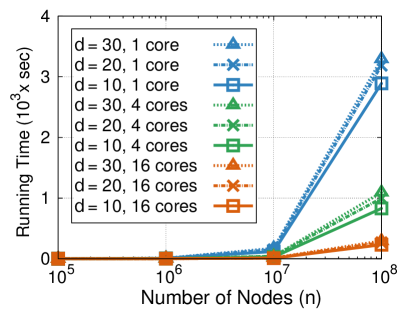
(a) Running time in linear

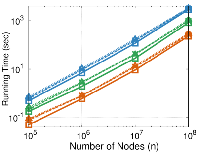
(b) Running time in log scale

Figure 4. Running time of SIEA on synthetic networks

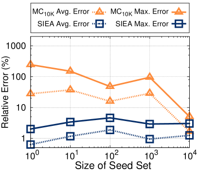
(a) Relative Error

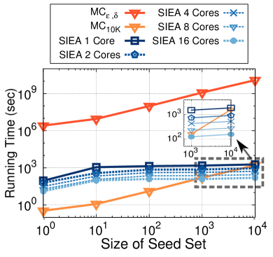
(b) Running Time

Figure 5. Comparing SIEA, MC${}_{\text{10K}}$ and MC_ϵ,δ on Twitter

Table 6. Comparing performance of algorithms in estimating influence spread in LT model (seed set size $|S|=1$)

	Avg. Rel. Error (%)				Max. Rel. Error (%)				Running time (sec.)
Dataset	$\textsf{SIEA}{}_{LT}$	MC${}_{\text{10K}}$	MC${}_{\text{100K}}$		$\textsf{SIEA}{}_{LT}$	MC${}_{\text{10K}}$	MC${}_{\text{100K}}$		$\textsf{SIEA}{}_{LT}$	$\textsf{SIEA}{}_{LT}$ (16 cores)	MC${}_{\text{10K}}$	MC${}_{\text{100K}}$	MCϵ,δ
NetHEP	1.6	1.6	0.6		8.4	7.9	2.5		0.0	0.0	0.0	0.1	1.0
NetPHY	1.2	0.5	0.3		12.7	4.4	1.4		0.0	0.0	0.0	0.1	2.9
Epinions	1.5	4.3	2.2		7.0	17.4	7.4		0.7	0.4	0.0	0.4	24.5
DBLP	0.4	1.0	0.5		5.7	11.4	2.2		2.4	0.4	0.3	2.5	1530.4
Orkut	0.5	3.3	1.1		1.9	22.1	5.9		249.4	25.0	8.5	84.2	$4.6\cdot 10^{4}$
Twitter	2.4	36.1	20.7		7.1	97.5	85.6		6820.0	548.6	32.2	287.6	$1.4\cdot 10^{7}$
Friendster	0.2	3.1	1.4		2.4	16.5	9.0		6183.9	701.8	20.4	137.8	$9.3\cdot 10^{6}$

6.4. Scalability Test

We test the scalability of the single core and parallel versions of our method on synthetic networks generated by the well-known GTgraph with various network sizes. We also carry the same tests on the real-world Twitter network in comparison with the MC.

6.4.1. On Synthetic Datasets

We generate synthetic graphs using GTgraph(Bader and Madduri, 2006), a standard graph generator used widely in large scale experiments on graph algorithms (Hong et al., 2011; Agarwal et al., 2010; Campan, 2008). We generate graphs with number of nodes $n\in\{10^{5},10^{6},10^{7},10^{8}\}$. For each size $n$, we generate 3 different graphs with average degree $d\in\{10,20,30\}$. We use the WC model to assign edge weights. We run SIEA with different number of cores $C=\{1,4,16\}$

Figure 4 reports the time SIEA spent to estimate influence spread of seed set of size 1. With the same number of nodes, we see that the running time of SIEA does not significantly increase as the average degree increases. Figure 4b views Figure 4a in logarithmic scale to show the linear increase of running time with respect to the increases of nodes. As expected, SIEA speeds up proportionally to number of cores used. As a result, SIEA with 16 cores is able to estimate influence spread of a random node on a synthetic graph of 100 million nodes and 1.5 billion of edges in just 5 minutes.

6.4.2. On Twitter Dataset

Figure 5 evaluates the performance of SIEA in comparison with MC${}_{\text{10K}}$ on various seed set sizes $|S|=\{1,10,100,1k,10k\}$ on Twitter dataset. On all the sizes of seed sets, SIEA consistently has average and maximum relative errors smaller than 10% (Figure 5a). The maximum relative error of MC${}_{\text{10K}}$ goes up to 244% with seed set size $|S|=1$. As observed in experiments with large size seed sets, both SIEA and MC${}_{\text{10K}}$ have similar error rate with seed set size $|S|=10000$.

In terms of running time, as the seed set size increases in powers of ten, SIEA’s running time increases in much lower pace, e.g. few hundreds of seconds, while MC_ϵ,δ consumes proportionally more time (Figure 5b). Figure 5b also evaluates parallel implementation of SIEA by varying number of CPU cores $C=\{1,2,4,8,16\}$. The running time of SIEA reduces almost two times every time the number of cores doubles confirming the almost linear speedup.

Altogether, the parallel implementation of SIEA shows a linear speedup behavior with respect to the number of cores used. On the same network with size of seed sets linearly grows, SIEA requires slightly more time to estimate influence spread while Monte-Carlo shows a linear runtime requirement. Throughout the experiments, SIEA always guarantees small error rate within $\epsilon$.

6.5. Influence Estimation under LT Model

We illustrate the generality of our algorithms in various diffusion model by adapting SIEA for the LT model by only replacing IICP with the sampling algorithm for the LT (Kempe et al., 2003). The algorithm is then named $\textsf{SIEA}{}_{LT}$. The setting is similar to the case of IC. We present the results of $\textsf{SIEA}{}_{LT}$ compared with MC${}_{\text{10K}}$, MC${}_{\text{100K}}$, MC_ϵ,δ in Table 6. INFEST is initially proposed for the IC model, thus, we results for INFEST under the LT model are not available.

The results are mostly consistent with those observed under the IC model. $\textsf{SIEA}{}_{LT}$ obtains significantly smaller errors and runs in order of magnitudes faster than the counterparts. The results again confirm that the estimation quality of MC using $10K$ samples is not good enough to be considered as gold-standard quality benchmark.

7. Related work

In a seminal paper (Kempe et al., 2003), Kempe et al. formulated and generalized two important influence diffusion models, i.e. Independent Cascade (IC) and Linear Threshold (LT). This work has motivated a large number of follow-up researches on information diffusion (Kempe et al., 2005; Chen et al., 2010; Borgs et al., 2014; Lucier et al., 2015; Cohen et al., 2014; Ohsaka et al., 2016) and applications in multiple disciplines (Leskovec et al., 2007; Ioannides and Datcher, 2004; Krause et al., 2008). Kempe et al. (Kempe et al., 2003) proved the monotonicity and submodularity properties of influence as a function of sets of nodes. Later, Chen et al. (Chen et al., 2010) proved that computing influence under these diffusion models is #P-hard.

Most existing works uses the naive influence cascade simulations to estimate influences (Kempe et al., 2003; Leskovec et al., 2007; Chen et al., 2010; Lucier et al., 2015). Most recently, Lucier et al. (Lucier et al., 2015) proposed an estimation algorithm with rigorous quality guarantee for a single seed set. The main idea is guessing a small interval of size $(1+\epsilon)$ that the true influence falls in and verifying whether the guess is right with high probability. However, their approach is not scalable due to a main drawback that the guessed intervals are very small, thus, the number of guesses as well as verifications made is huge. As a result, the method in (Lucier et al., 2015) can only run for small dataset and still takes hours to estimate a single seed set. They also developed a distributed version on MapReduce however, graph algorithms on MapReduce have various serious issues (Gupta et al., 2013; Lin and Schatz, 2010).

Influence estimation oracles are developed in (Cohen et al., 2014; Ohsaka et al., 2016) which take advantage of sketching the influence to preprocess the graph for fast queries. Cohen et al. (Cohen et al., 2014) use the novel bottom-$k$ min-hash sketch to build combined reachability sketches while Ohsaka et al. in (Ohsaka et al., 2016) adopt the reverse influence sketches. (Ohsaka et al., 2016) also introduces the reachability-true-based technique to deal with dynamic changes in the graphs. However, these methods require days for preprocessing in order to achieve fast responses for multiple queries.

There have also been increasing interests in many related problems. (Cha et al., 2009; Goyal et al., 2010) focus on designing data mining or machine learning algorithms to extract influence cascade model parameters from real datasets, e.g. action logs. Influence Maximization, which finds a seed set of certain size with the maximum influence among those in the same size, found many real-world applications and has attracted a lot of research work (Kempe et al., 2003; Leskovec et al., 2007; Chen et al., 2010; Nguyen et al., 2013; Borgs et al., 2014; Tang et al., 2015; Nguyen et al., 2016a, b).

8. Conclusion

This paper investigates a new measure, called Outward Influence, for nodes’ influence in social networks. Outward influence inspires new statiscal algorithms, namely Importance IC Polling (IICP) and Robust Mean Estimation (RSA) to estimate influence of nodes under various stochastic diffusion models. Under the popular IC model, the IICP leads to an FPRAS for estimating outward influence and SIEA to estimate influence spread. SIEA is $\Omega(\log^{4}(n))$ times faster than the most recent state-of-the-art and experimentally outperform the other methods by several orders of magnitudes. As previous approaches to compute ground truth influence can result in high error and long computational time, our algorithms provides concrete and scalable tools to estimate ground-truth influence for research on network cascade and social influence.

Proof of Lemma 1

Recall that on a sampled graph $g\sim\mathcal{G}$, for a set $S\subseteq V$, we denote $r^{(o)}_{g}(S)$ to be the set of nodes, excluding the ones in $S$, that are reachable from $S$ through live edges in $g$, i.e. $r^{(o)}_{g}(S)=r_{g}(S)\backslash S$. Alternatively, $r^{(o)}_{g}(S)$ is called the outward influence cascade of $S$ on sample graph $g$ and, consequently, we have,

(31) $$\mathbb{I}_{out}(S)=\sum_{g\sim\mathcal{G}}|r^{(o)}_{g}(S)|\Pr[g\sim\mathcal{G}].$$

It is sufficient to show that $|r^{(o)}_{g}(S)|$ is submodular, as $\mathbb{I}_{out}(S)$ is a linear combination of submodular functions. Consider a sample graph $g\sim\mathcal{G}$, two sets $S,T$ such that $S\subseteq T\subseteq V$ and $v\in V\backslash T$. We have three possible cases:

• Case $v\in r^{(o)}_{g}(S)$: then $v\in r^{(o)}_{g}(T)$ since $S\subseteq T$ and $v\notin T$. Thus, we have the following,

  $$r^{(o)}_{g}(S\cup\{v\})-r^{(o)}_{g}(S)$$

  (32) $$\qquad\qquad=r^{(o)}_{g}(T\cup\{v\})-r^{(o)}_{g}(T)=-1.$$

• Case $v\notin r^{(o)}_{g}(S)$ but $v\in r^{(o)}_{g}(T)$: We have that,

  $$r^{(o)}_{g}(S\cup\{v\})-r^{(o)}_{g}(S)$$

  (33) $$\qquad\qquad=|r^{(o)}_{g}(\{v\})\backslash(r^{(o)}_{g}(S)\cup S)|\geq 0,$$

  while $r^{(o)}_{g}(T\cup\{v\})-r^{(o)}_{g}(T)=-1$. Thus,

  $$r^{(o)}_{g}(S\cup\{v\})-r^{(o)}_{g}(S)$$

  (34) $$\qquad\qquad>r^{(o)}_{g}(T\cup\{v\})-r^{(o)}_{g}(T).$$

• Case $v\notin r^{(o)}_{g}(T)$: Since $\forall u\in r^{(o)}_{g}(S)\cup S$, we have either $u\in r^{(o)}_{g}(T)$ or $u\in T$ or $r^{(o)}_{g}(S)\cup S\subseteq r^{(o)}_{g}(T)\cup T$, and thus,

  $$r^{(o)}_{g}(S\cup\{v\})-r^{(o)}_{g}(S)$$

  $$\qquad\qquad=|r^{(o)}_{g}(\{v\})\backslash(r^{(o)}_{g}(S)\cup S)|$$

  $$\qquad\qquad\geq|r^{(o)}_{g}(\{v\})\backslash(r^{(o)}_{g}(T)\cup T)|$$

  (35) $$\qquad\qquad=r^{(o)}_{g}(T\cup\{v\})-r^{(o)}_{g}(T).$$

In all three cases, we have,

$$r^{(o)}_{g}(S\cup\{v\})-r^{(o)}_{g}(S)$$

(36) $$\qquad\geq r^{(o)}_{g}(T\cup\{v\})-r^{(o)}_{g}(T).$$

Applying Eq. Proof of Lemma 1 on all possible $g\sim\mathcal{G}$ and taking the sum over all of these inequalities give

$$\sum_{g\sim\mathcal{G}}(r^{(o)}_{g} (S\cup\{v\})-r^{(o)}_{g}(S))\Pr[g\sim\mathcal{G}]$$

$$\geq\sum_{g\sim\mathcal{G}}(r^{(o)}_{g}(T\cup\{v\})-r^{(o)}_{g}(T))\Pr[g\sim\mathcal{G}],$$

or,

(37) $$\mathbb{I}_{out}(S\cup\{v\})-\mathbb{I}_{out}(S)\geq\mathbb{I}_{out}(T\cup\{v\})-\mathbb{I}_{out}(T).$$

That completes the proof.

Proof of Lemma 4

Let $\Omega^{+}_{W}$ be the probability space of all possible cascades from $S$. For any cascade $W^{(S)}{}\supseteq S$, the probability of that cascade in $\Omega^{+}_{W}$ is given by

$$\Pr[W^{(S)}{}\in\Omega^{+}_{W}]=\sum_{g\in\Omega_{\mathcal{G}},g\leadsto W^{(S)}{}}\Pr[g\in\Omega_{\mathcal{G}}],$$

where $g\leadsto W^{(S)}{}$ means that $W^{(S)}{}$ is the set of reachable nodes from $S$ in $g$.

Let $\Omega_{W}$ be the probability space of non-trivial cascades. According to the Stage 1 in IICP, the probability of the trivial cascade is:

$$\Pr[S\in\Omega_{W}]=0.$$

Comparing to the mass of cascades in $\Omega^{+}_{W}$, the probability mass of the trivial cascade $S$ in $\Omega_{W}$ is redistributed proportionally to other cascades in $\Omega_{W}$. Specifically, according to line 2 in IICP, the probability mass of all the non-trivial cascades in $\Omega_{W}$ is multiplied by a factor $1/\beta_{0}$. Thus,

$$\Pr[W^{(S)}{}\in\Omega^{+}_{W}]=\Pr[W^{(S)}{}\in\Omega_{W}]\cdot\beta_{0}\ \ \forall W^{(S)}{}\neq S.$$

It follows that

(38) $$\mathbb{I}_{out}(S) =\sum_{W^{(S)}{}\in\Omega^{+}_{W}}|W^{(S)}{}\setminus S|\cdot\Pr[W^{(S)}{}\in\Omega^{+}_{W}]$$

(39) $$=\sum_{W^{(S)}{}\in\Omega_{W}}|W^{(S)}{}\setminus S|\cdot\Pr[W^{(S)}{}\in\Omega^{W}]\beta_{0}$$

(40) $$=\mathbb{E}[|W^{(S)}{}|]\cdot\beta_{0}=\mathbb{E}[Y^{(S)}{}]\cdot\beta_{0}.$$

We note that for $W^{(S)}{}=S$, $|W^{(S)}{}\setminus S|=0$. Thus the difference in the probability masses between the two probabilistic spaces does not affect the 2nd step.

Proof of Theorem 4.1

We will equivalently prove two probabilistic inequalities:

(41) $$\Pr[\hat{\mu}_{X}<(1-\epsilon)\mu_{X}]\leq\frac{\delta}{2},$$

and

(42) $$\Pr[\hat{\mu}_{X}>(1+\epsilon)\mu_{X}]\leq\frac{\delta}{2}.$$

Prove Eq. 41. We first realize that at termination point of Alg. 2, due to the stopping condition $h=\sum_{j=1}^{T}X_{j}\geq\Upsilon$ and $X_{j}\leq b,\forall j$, the following inequalities hold,

(43) $$\Upsilon\leq\sum_{j=1}^{T}X_{j}\leq\Upsilon+b.$$

The left hand side of Eq. 41 is rewritten as follows,

(44) $$\Pr[\hat{\mu}_{X}<(1-\epsilon)\mu_{X}] =\Pr\Big{[}\frac{\sum_{j=1}^{T}X_{j}}{T}<(1-\epsilon)\mu_{X}\Big{]}$$

(45) $$=\Pr\Big{[}\sum_{j=1}^{T}X_{j}<(1-\epsilon)\mu_{X}T\Big{]}$$

(46) $$\leq\Pr[\Upsilon<(1-\epsilon)\mu_{X}T].$$

The last inequality is due to our realization in Eq. 43. Assume that $\epsilon<1$ and $\mu_{X}>0$, let denote $L_{1}=\lceil\frac{\Upsilon}{(1-\epsilon)\mu_{X}}\rceil$. We then have,

(47) $$L_{1}\geq\frac{\Upsilon}{(1-\epsilon)\mu_{X}}\Rightarrow\frac{\Upsilon}{L_{1}}\leq(1-\epsilon)\mu_{X},$$

and

(48) $$L_{1}>\frac{\Upsilon}{\mu_{X}}>(2+\frac{2}{3}\epsilon)\ln(\frac{2}{\delta})\frac{1}{\epsilon^{\prime 2}\mu_{X}}(b-a).$$

Thus, from Eq. 46, we obtain,

$$\Pr[\hat{\mu}_{X}<(1-\epsilon)\mu_{X}] \leq\Pr[L_{1}\leq T]=\Pr\Big{[}\sum_{j=1}^{L_{1}}X_{j}\leq\sum_{j=1}^{T}X_{j}\Big{]}$$

(49) $$\leq\Pr\Big{[}\sum_{j=1}^{L_{1}}X_{j}\leq\Upsilon+b\Big{]}$$

(50) $$\leq\Pr\Big{[}\frac{\sum_{j=1}^{L_{1}}X_{j}}{L_{1}}\leq\frac{\Upsilon+b}{L_{1}}\Big{]},$$

where the second inequality is due to Eq. 43. Note that $\frac{\sum_{j=1}^{L_{1}}X_{j}}{L_{1}}$ is an estimate of $\mu_{X}$ using the first $L_{1}$ random variables $X_{1},\dots,X_{L_{1}}$. Furthermore, from Eq. 47 that $\frac{\Upsilon}{L_{1}}\leq(1-\epsilon)\mu_{X}$, we have,

(51) $$\frac{\Upsilon+b}{L_{1}}\leq(1-\epsilon)\mu_{X}+\frac{b}{L_{1}}=(1-\epsilon+\frac{b}{L_{1}\mu_{X}})\mu_{X}.$$

Since $L_{1}>(2+\frac{2}{3}\epsilon)\ln(\frac{2}{\delta})\frac{1}{\epsilon^{\prime 2}\mu_{X}}(b-a)$ from Eq. 48,

(52) $$\frac{\Upsilon+b}{L_{1}}\leq\Big{(}1-\epsilon+\frac{\epsilon^{2}b}{(2+\frac{2}{3}\epsilon)\ln(\frac{2}{\delta})(b-a)}\Big{)}\mu_{X}=(1-\epsilon^{\prime})\mu_{X}.$$

Plugging these into Eq. 50, we obtain,

(53) $$\Pr[\hat{\mu}_{X}<(1-\epsilon)\mu_{X}] \leq\Pr\Big{[}\sum_{j=1}^{L_{1}}X_{j}\leq(1-\epsilon^{\prime})\mu_{X}L_{1}\Big{]}.$$

Now, apply the Chernoff-like bound in Eq. 23 with $T=L_{1}$ and note that $L_{1}>(2+\frac{2}{3}\epsilon)\ln(\frac{2}{\delta})\frac{1}{\epsilon^{\prime 2}\mu_{X}}(b-a)>2\ln(\frac{2}{\delta})\frac{1}{\epsilon^{\prime 2}\mu_{X}}(b-a)$, we achieve,

(54) $$\Pr[\hat{\mu}_{X}<(1-\epsilon)\mu_{X}] \leq\exp\Big{(}-\frac{\epsilon^{\prime 2}L_{1}\mu_{X}}{2(b-a)}\Big{)}$$

$$\leq\exp\Big{(}-\frac{\epsilon^{\prime 2}2\ln(\frac{2}{\delta})\frac{1}{\epsilon^{\prime 2}\mu_{X}}(b-a)}{2(b-a)}\Big{)}$$

(55) $$=\frac{\delta}{2}.$$

That completes the proof of Eq. 41.

Prove Eq. 42. The left hand side of Eq. 42 is rewritten as follows,

(56) $$\Pr[\hat{\mu}_{X}>(1+\epsilon)\mu_{X}] =\Pr\Big{[}\sum_{j=1}^{T}X_{j}>(1+\epsilon)\mu_{X}T\Big{]}$$

(57) $$\leq\Pr[\Upsilon+b>(1+\epsilon)\mu_{X}T],$$

where the last inequality is due to our observation that $\sum_{j=1}^{T}X_{j}\leq\Upsilon+b$. Under the same assumption that $0<\mu_{X}\leq\frac{b}{1+\epsilon}$, we denote $L_{2}=\lfloor\frac{\Upsilon+b}{(1+\epsilon)\mu_{X}}\rfloor$. We then have,

(58) $$L_{2}\geq\frac{\Upsilon}{(1+\epsilon)\mu_{X}}=(2+\frac{2}{3}\epsilon)\ln(\frac{2}{\delta})\frac{1}{\epsilon^{\prime 2}\mu_{X}}(b-a),$$

and

(59) $$L_{2}\leq\frac{\Upsilon+b}{(1+\epsilon)\mu_{X}}\Rightarrow\frac{\Upsilon+b}{L_{2}}\geq(1+\epsilon)\mu_{X}$$

(60) $$\Rightarrow\text{ } \frac{\Upsilon}{L_{2}}\geq(1+\epsilon)\mu_{X}-\frac{b}{L_{2}}=(1+\epsilon-\frac{b}{L_{2}\mu_{X}})\mu_{X}$$

(61) $$\Rightarrow\text{ } \frac{\Upsilon}{L_{2}}\geq\Big{(}1+\epsilon-\frac{\epsilon^{2}b}{(2+\frac{2}{3}\epsilon)\ln(\frac{2}{\delta})(b-a)}\Big{)}\mu_{X}=(1+\epsilon^{\prime})\mu_{X}$$

Thus, from Eq. 57, we obtain,

$$\Pr[\hat{\mu}_{X}> (1+\epsilon)\mu_{X}]\leq\Pr[L_{2}\geq T]=\Pr\Big{[}\sum_{j=1}^{L_{2}}X_{j}\geq\sum_{j=1}^{T}X_{j}\Big{]}$$

(62) $$\leq\Pr\Big{[}\sum_{j=1}^{L_{2}}X_{j}\geq\Upsilon\Big{]}=\Pr\Big{[}\frac{\sum_{j=1}^{L_{2}}X_{j}}{L_{2}}\geq\frac{\Upsilon}{L_{2}}\Big{]}$$

(63) $$\leq\Pr\Big{[}\frac{\sum_{j=1}^{L_{2}}X_{j}}{L_{2}}\geq(1+\epsilon^{\prime})\mu_{X}\Big{]}$$

where the last inequality follows from Eq. 61. By applying another Chenoff-like bound from Eq. 22 combined with the lower bound on $L_{2}$ in Eq. 58, we achieve,

(64) $$\Pr[\hat{\mu}_{X}>(1+\epsilon)\mu_{X}]\leq\exp\big{(}-\frac{\epsilon^{\prime 2}L_{2}\mu_{X}}{(2+\frac{2}{3}\epsilon)(b-a)}\big{)}=\frac{\delta}{2},$$

which completes the proof of Eq. 42.

Follow the same procedure as in the proof of Eq. 42, we obtain the second statement in the theorem that,

(65) $$\Pr[T\leq(1+\epsilon)\Upsilon/\mu_{X}]>1-\delta/2,$$

which completes the proof of the whole theorem.

More elaboration on the hold in (Dagum et al., 2000). The stopping rule algorithm in (Dagum et al., 2000) is described in Alg. 6.

Input: Random variables $X_{1},X_{2},\dots$ and $0<\epsilon,\delta<1$

Output: An $(\epsilon,\delta)$-approximate of $\mu_{X}=E[X_{i}]$

1 Compute: $\Upsilon_{1}=1+(1+\epsilon)4(e-2)\ln(\frac{2}{\delta})\frac{1}{\epsilon^{2}}$;

2 Initialize $h=0,T=0$;

3 while $h<\Upsilon_{1}$ do

4       $h\leftarrow h+X_{T},T\leftarrow T+1$;

5      

return $\hat{\mu}_{X}=\Upsilon_{1}/T$;

Algorithm 6 Stopping Rule Algorithm (Dagum et al., 2000)

The algorithm first computes $\Upsilon_{1}$ and then, generates samples $X_{j}$ until the sum of their outcomes exceed $\Upsilon_{1}$. Afterwards, it returns $\Upsilon_{1}/T$ as the estimate. Apparently, $\Upsilon_{1}/T$ is a biased estimate of $\mu_{X}$ since $\sum_{j=1}^{T}X_{j}\geq\Upsilon_{1}$.

An important realization for this algorithm from our proof of Theorem 4.1 is that $\Upsilon_{1}\leq\sum_{j=1}^{T}X_{j}\leq\Upsilon_{1}+b$ with $b=1$ for $[0,1]$ random variables. In section 5 of (Dagum et al., 2000), following the proof of $\Pr[\hat{\mu}_{X}>(1+\epsilon)\mu_{X}]\leq\delta/2$ to prove $\Pr[\hat{\mu}_{X}<(1-\epsilon)\mu_{X}]\leq\delta/2$, there is step that derives as follows: $\Pr[L_{1}\leq T]=\Pr\left[\sum_{j=1}^{L_{1}}X_{j}\leq\sum_{j=1}^{T}X_{j}\right]=\Pr\left[\sum_{j=1}^{L_{1}}X_{j}\leq\Upsilon_{1}\right]$ where $L_{1}$ is a predefined number, i.e. $L_{1}=\lfloor\frac{\Upsilon_{1}}{(1-\epsilon)\mu_{X}}\rfloor$. However, since $\Upsilon_{1}\leq\sum_{j=1}^{T}X_{j}\leq\Upsilon_{1}+b$, the last equality does not hold. This is based on Eq. 49 with the correct expression being $\Pr\Big{[}\sum_{j=1}^{L_{1}}X_{j}\leq\Upsilon+b\Big{]}$ instead of $\Pr\Big{[}\sum_{j=1}^{L_{1}}X_{j}\leq\Upsilon\Big{]}$.

Proof of Theorem 4.2

[Proof of Part (1)] If $\epsilon\geq 1/4$, then RSA only runs GSRA and hence, from Theorem 4.1, the returned solution satisfies the precision requirement. Otherwise, since the first steps is literally applying GSRA with $\sqrt{\epsilon}<1/2,\delta/3$, we have,

(66) $$\Pr[\mu_{X}(1-\sqrt{\epsilon})\leq\hat{\mu}^{\prime}_{X}\leq\mu_{X}(1+\sqrt{\epsilon})]\geq 1-\delta/3$$

We prove that in step 2, $\hat{\rho}_{X}\geq\rho_{X}/2$. Let define the random variables $\xi_{i}=(X^{\prime}_{2i-1}-X^{\prime}_{2i})^{2}/2,i=1,2,\dots$ and thus, $\mathbb{E}[\xi_{i}]=\mathrm{Var}[X]$. Consider the following two cases.

1. If $\mathrm{Var}[X]\geq\epsilon\mu_{X}(b-a)$, consider two sub-cases:

   1. If $\mathrm{Var}[X]\geq 2(1-\sqrt{\epsilon})\epsilon\mu_{X}(b-a)$, then since $N_{\sigma}=\Upsilon_{2}\epsilon/\hat{\mu}^{\prime}_{X}\geq\frac{2}{1-\sqrt{\epsilon}}(1+\ln(\frac{3}{2})/\ln(\frac{2}{\delta}))\Upsilon\epsilon/\mu_{X}$, applying the Chernoff-like bound in Eq. 21 gives,

      (67) $$\Pr[\mathrm{Var}[X]/2\leq\Delta/N_{\sigma}]\geq 1-\delta/3$$

      Thus, $\hat{\rho}_{X}\geq\mathrm{Var}[X]/2=\rho_{X}/2$ with a probability of at least $1-\delta/3$.

   2. If $\mathrm{Var}[X]\leq 2(1-\sqrt{\epsilon})\epsilon\mu_{X}(b-a)$, then $\epsilon\mu_{X}(b-a)\geq\mathrm{Var}[X]/(2(1-\sqrt{\epsilon}))$ and therefore, $\hat{\rho}_{X}\geq\epsilon\hat{\mu}^{\prime}_{X}(b-a)\geq(1-\sqrt{\epsilon})\epsilon\mu_{X}(b-a)\geq\mathrm{Var}_{X}/2=\rho_{X}/2$.

2. If $\mathrm{Var}[X]\leq\epsilon\mu_{X}(b-a)$, it follows that $\hat{\rho}_{X}\geq\epsilon\hat{\mu}_{X}\geq\rho_{X}(1-\min\{\sqrt{\epsilon},1/2\})$ with probability at least $1-\delta/3$.

Thus, after steps 1 and 2, $2\frac{1+\sqrt{\epsilon}}{1-\sqrt{\epsilon}}\hat{\rho}_{X}/{\hat{\mu}}^{\prime 2}_{X}\geq\rho_{X}/\mu^{2}_{Z}$ with probability at least $1-\delta/3$. In step 3, since $T=\Upsilon_{2}\hat{\rho}_{X}/({\hat{\mu}}^{\prime 2}_{X}(b-a))\geq(1+\ln(\frac{3}{2})/\ln(\frac{2}{\delta}))\Upsilon\rho_{X}/(\mu^{2}_{X}(b-a))$ and hence, applying the Chernoff-like bound in Eq. 24 again gives,

(68) $$\Pr[\mu_{X}(1-\epsilon)\leq\hat{\mu}_{X}\leq\mu_{X}(1+\epsilon)]\geq 1-2\delta/3.$$

Accumulating the probabilities, we finally obtain,

(69) $$\Pr[\mu_{X}(1-\epsilon)\leq\hat{\mu}_{X}\leq\mu_{X}(1+\epsilon)]\geq 1-\delta,$$

This completes the proof of part (1).

[Proof of Part (2)] The RSA algorithm may fail to terminate after using $\mathcal{O}(\Upsilon\rho_{X}/(\mu^{2}_{X}(b-a)))$ samples if either:

1. The GSRA algorithm fails to return an $(\sqrt{\epsilon},\delta/3)$-approximate $\hat{\mu}^{\prime}_{X}$ with probability at most $\delta/2$, or,

2. In step 2, for $\mathrm{Var}[X]\leq 2(1-\sqrt{\epsilon})\epsilon\mu_{X}(b-a)$, $\hat{\rho}_{X}$ is not $\mathcal{O}(\epsilon\mu_{X}(b-a))$ with probability at most $\delta/2$.

From Theorem 4.1, with $T=(1+\epsilon)\Upsilon/\mu_{X}=\mathcal{O}(\Upsilon\rho_{X}/(\mu^{2}_{X}(b-a)))$, the first case happens with probability at most $\delta/2$. In addition, we can show similarly to Theorem 4.1 that if $\mathrm{Var}[X]\leq 2\epsilon\mu_{X}(b-a)$, then,

(70) $$\Pr[\Delta/T\geq 4\epsilon\mu_{X}(b-a)]\leq\exp(-T\epsilon\mu_{X}(b-a)/2).$$

Thus, for $T\geq 2\Upsilon\epsilon/\mu_{X}$, we have $\Pr[\Delta/T\geq 4\epsilon\mu_{X}]\leq\delta/2$.

Proof of Lemma 6

We start with the computation of $\mathrm{Var}[Z^{(S)}]$ with a note that $\mathbb{E}[Z^{(S)}]=\mathbb{I}(S)$,

$$\mathrm{Var}[Z^{(S)}]=\sum_{z=\beta_{0}+|S|}^{(n-|S|)\beta_{0}+|S|}(z-\mathbb{E}[Z^{(S)}])^{2}\Pr[Z^{(S)}=z]$$

$$=\sum_{y=1}^{n-|S|}(y\beta_{0}+|S|-\mathbb{I}(S))^{2}\Pr[Y^{(S)}=y]$$

$$=\sum_{y=1}^{n-|S|}(y\beta_{0}-\mathbb{I}_{out}(S)\beta_{0}+\mathbb{I}_{out}(S)\beta_{0}+|S|-\mathbb{I}(S))^{2}\Pr[Y^{(S)}=y]$$

$$=\beta_{0}^{2}\sum_{y=1}^{n-|S|}(y-\mathbb{I}_{out}(S))^{2}\Pr[Y^{(S)}=y]$$

$$\text{ \ }+\sum_{y=1}^{n-|S|}(\mathbb{I}_{out}(S)\beta_{0}+|S|-\mathbb{I}(S))^{2}\Pr[Y^{(S)}=y]$$

$$\text{ \ }+2\beta_{0}\sum_{y=1}^{n-|S|}(y-\mathbb{I}_{out}(S))(\mathbb{I}_{out}(S)\beta_{0}+|S|-\mathbb{I}(S))\Pr[Y^{(S)}=y]$$

Since $Y^{(S)}\geq 1$ and $\Pr[Y^{(S)}=y]=\frac{\Pr[M^{(S)}=y+|S|]}{\beta_{0}}$, we have,

$$\sum_{y=1}^{n-|S|}(y-\mathbb{I}_{out}(S))^{2}\Pr[Y^{(S)}=y]$$

$$\qquad=\frac{1}{\beta_{0}}\sum_{m=1+|S|}^{n}(m-\mathbb{E}[M^{(S)}])^{2}\Pr[M^{(S)}=m]$$

$$\qquad=\frac{1}{\beta_{0}}\sum_{m=|S|}^{n}(m-\mathbb{E}[M^{(S)}])^{2}\Pr[M^{(S)}=m]-\frac{1}{\beta_{0}}\mathbb{I}_{out}^{2}(S)(1-\beta_{0})$$

(71) $$\qquad=\frac{1}{\beta_{0}}(\mathrm{Var}[M^{(S)}]-\mathbb{I}_{out}^{2}(S)(1-\beta_{0})),$$

and,

$$\sum_{y=1}^{n-|S|}\beta_{0}(y-\mathbb{I}_{out}(S))(\mathbb{I}_{out}(S)\beta_{0}+|S|-\mathbb{I}(S))\Pr[Y^{(S)}=y]$$

$$=(\mathbb{I}_{out}(S)\beta_{0}+|S|-\mathbb{I}(S))\sum_{y=1}^{n-|S|}(y-\mathbb{I}_{out}(S))\Pr[Y^{(S)}=y]$$

(72) $$=(\mathbb{I}_{out}(S)\beta_{0}+|S|-\mathbb{I}(S))\mathbb{I}_{out}(S)(1/\beta_{0}-1).$$

Plug these back in the $\mathrm{Var}[Z^{(S)}]$, we obtain,

$$\mathrm{Var}[Z^{(S)}] =\beta_{0}(\mathrm{Var}[M^{(S)}]-\mathbb{I}_{out}^{2}(S)(1-\beta_{0}))$$

$$\qquad+(\mathbb{I}_{out}(S)\beta_{0}+|S|-\mathbb{I}(S))^{2}$$

$$\qquad+2\beta_{0}(\mathbb{I}_{out}(S)\beta_{0}+|S|-\mathbb{I}(S))\mathbb{I}_{out}(S)(1/\beta_{0}-1)$$

(73) $$=\beta_{0}\cdot\mathrm{Var}[M^{(S)}]-(1-\beta_{0})\mathbb{I}_{out}^{2}(S)$$

That completes the computation.

References

- (1)
- Agarwal et al. (2010) V. Agarwal, F. Petrini, D. Pasetto, and D. A. Bader. 2010. Scalable graph exploration on multicore processors. In SC. IEEE, 1–11.
- Bader and Madduri (2006) D. A. Bader and K. Madduri. 2006. Gtgraph: A synthetic graph generator suite. Atlanta, GA, February (2006).
- Borgs et al. (2014) C. Borgs, M. Brautbar, J. Chayes, and B. Lucier. 2014. Maximizing Social Influence in Nearly Optimal Time. In SODA. SIAM, 946–957.
- Campan (2008) A. Campan. 2008. A clustering approach for data and structural anonymity in social networks. PinKDD (2008), 54.
- Cha et al. (2009) M. Cha, A. Mislove, and K. P. Gummadi. 2009. A measurement-driven analysis of information propagation in the flickr social network. In WWW. ACM, 721–730.
- Chen et al. (2010) W. Chen, C. Wang, and Y. Wang. 2010. Scalable influence maximization for prevalent viral marketing in large-scale social networks. In KDD. ACM, 1029–1038.
- Chung and Lu (2006) F. Chung and L. Lu. 2006. Concentration inequalities and martingale inequalities: a survey. Internet Mathematics (2006), 79–127.
- Cohen et al. (2014) E. Cohen, D. Delling, T. Pajor, and R. F. Werneck. 2014. Sketch-based influence maximization and computation: Scaling up with guarantees. In CIKM. ACM, 629–638.
- Dagum et al. (2000) P. Dagum, R. Karp, M. Luby, and S. Ross. 2000. An Optimal Algorithm for Monte Carlo Estimation. SICOMP (2000), 1484–1496.
- Daley et al. (2001) D. J. Daley, J. Gani, and J. M. Gani. 2001. Epidemic modelling: an introduction. Vol. 15. Cambridge University Press.
- Dinh and Thai (2015) T. N. Dinh and M. T. Thai. 2015. Assessing attack vulnerability in networks with uncertainty. In INFOCOM. IEEE, 2380–2388.
- Du et al. (2013) N. Du, L. Song, M. Gomez-Rodriguez, and H. Zha. 2013. Scalable influence estimation in continuous-time diffusion networks. In NIPS. 3147–3155.
- Goyal et al. (2010) A. Goyal, F. Bonchi, and L. V. S. Lakshmanan. 2010. Learning Influence Probabilities in Social Networks. In WSDM. ACM, 241–250.
- Gupta et al. (2013) P. Gupta, A. Goel, J. Lin, A. Sharma, D. Wang, and R. Zadeh. 2013. Wtf: The who to follow service at twitter. In WWW. ACM, 505–514.
- Hong et al. (2011) S. Hong, Sang K. Kim, T. Oguntebi, and K. Olukotun. 2011. Accelerating CUDA graph algorithms at maximum warp. In SIGPLAN Notices. ACM, 267–276.
- Ioannides and Datcher (2004) Y. M. Ioannides and L. L. Datcher. 2004. Job information networks, neighborhood effects, and inequality. Journal of economic literature (2004), 1056–1093.
- Kempe et al. (2003) D. Kempe, J. Kleinberg, and É. Tardos. 2003. Maximizing the spread of influence through a social network. In KDD. 137–146.
- Kempe et al. (2005) D. Kempe, J. Kleinberg, and E. Tardos. 2005. Influential nodes in a diffusion model for social networks. In ICALP. 1127–1138.
- Krause et al. (2008) A. Krause, A. Singh, and C. Guestrin. 2008. Near-optimal sensor placements in Gaussian processes: Theory, efficient algorithms and empirical studies. JMLR (2008), 235–284.
- Kwak et al. (2010) H. Kwak, C. Lee, H. Park, and S. Moon. 2010. What is Twitter, a social network or a news media?. In WWW. ACM, 591–600.
- Leskovec et al. (2007) J. Leskovec, A. Krause, C. Guestrin, C. Faloutsos, J. VanBriesen, and N. Glance. 2007. Cost-effective outbreak detection in networks. In KDD. ACM, 420–429.
- Lin and Schatz (2010) J. Lin and M. Schatz. 2010. Design patterns for efficient graph algorithms in MapReduce. In MLG. ACM, 78–85.
- Lucier et al. (2015) B. Lucier, J. Oren, and Y. Singer. 2015. Influence at scale: Distributed computation of complex contagion in networks. In KDD. ACM, 735–744.
- Mitzenmacher and Upfal (2005) M. Mitzenmacher and E. Upfal. 2005. Probability and computing: Randomized algorithms and probabilistic analysis. Cambridge University Press.
- Nguyen et al. (2013) D. T. Nguyen, Z. Huiyuan, S. Das, M. T. Thai, and T. N. Dinh. 2013. Least Cost Influence in Multiplex Social Networks: Model Representation and Analysis. In ICDM. 567–576.
- Nguyen et al. (2016) H. T. Nguyen, P. Ghosh, M. L. Mayo, and T. N. Dinh. 2016. Multiple Infection Sources Identification with Provable Guarantees. In CIKM. ACM, 1663–1672.
- Nguyen et al. (2016a) H. T. Nguyen, M. T. Thai, and T. N. Dinh. 2016a. Cost-aware targeted viral marketing in billion-scale networks. In INFOCOM. IEEE, 1–9.
- Nguyen et al. (2016b) H. T. Nguyen, M. T. Thai, and T. N. Dinh. 2016b. Stop-and-Stare: Optimal Sampling Algorithms for Viral Marketing in Billion-scale Networks. In SIGMOD. ACM, 695–710.
- Ohsaka et al. (2016) N. Ohsaka, T. Akiba, Y. Yoshida, and K. Kawarabayashi. 2016. Dynamic influence analysis in evolving networks. VLDB (2016), 1077–1088.
- Preciado et al. (2013) V. M. Preciado, M. Zargham, C. Enyioha, A. Jadbabaie, and G. Pappas. 2013. Optimal vaccine allocation to control epidemic outbreaks in arbitrary networks. In CDC. IEEE, 7486–7491.
- Tang et al. (2015) Y. Tang, Y. Shi, and X. Xiao. 2015. Influence Maximization in Near-Linear Time: A Martingale Approach. In SIGMOD. ACM, 1539–1554.
- Tang et al. (2014) Y. Tang, X. Xiao, and Y. Shi. 2014. Influence maximization: Near-optimal time complexity meets practical efficiency. In SIGMOD. ACM, 75–86.