Impact of basic angle variations on the parallax zero point for a scanning astrometric satellite

Abstract

Context. Determination of absolute parallaxes by means of a scanning astrometric satellite such as Hipparcos or Gaia relies on the short-term stability of the so-called basic angle between the two viewing directions. Uncalibrated variations of the basic angle may produce systematic errors in the computed parallaxes.

Aims. We examine the coupling between a global parallax shift and specific variations of the basic angle, namely those related to the satellite attitude with respect to the Sun.

Methods. The changes in observables produced by small perturbations of the basic angle, attitude, and parallaxes are calculated analytically. We then look for a combination of perturbations that has no net effect on the observables.

Results. In the approximation of infinitely small fields of view, it is shown that certain perturbations of the basic angle are observationally indistinguishable from a global shift of the parallaxes. If such perturbations exist, they cannot be calibrated from the astrometric observations but will produce a global parallax bias. Numerical simulations of the astrometric solution, using both direct and iterative methods, confirm this theoretical result. For a given amplitude of the basic angle perturbation, the parallax bias is smaller for a larger basic angle and a larger solar aspect angle. In both these respects Gaia has a more favourable geometry than Hipparcos. In the case of Gaia, internal metrology is used to monitor basic angle variations. Additionally, Gaia has the advantage of detecting numerous quasars, which can be used to verify the parallax zero point.

1 Introduction

The European Space Agency’s space astrometry mission Gaia, aiming to determine astrometric parameters for at least one billion stars with accuracies reaching 10 microarcseconds (de Bruijne, 2012), was launched in December 2013 (Gaia Collaboration et al., 2016b). Gaia is based on similar observation principles as the highly successful pioneering astrometric mission Hipparcos (ESA, 1997). In particular, both satellites use an optical system providing two viewing directions separated by a wide angle, referred to as the basic angle (Perryman et al., 2001). The goal of the present paper is to show how certain time-dependent variations of the basic angle can bias the parallax zero point of an astrometric solution derived from observations by such a scanning astrometric satellite.

The data processing for an astrometric satellite should, as far as possible, be based on the principle of self-calibration (Lindegren & Bastian, 2011). This means that the same observational data are used to determine both the scientifically interesting astrometric parameters and the so-called “nuisance parameters” that describe the instrument calibration, satellite attitude, and other relevant parts of the observation model (Lindegren et al., 2012). The self-calibration is, however, of limited applicability when variations of different parameters do not produce fully independent effects in the observables. Such situations can occur when the variation of certain parameters leads to changes in the observables that resemble the changes produced by the variation of some other parameters. The more similar the changes in the observables are, the stronger the correlation between the parameters. If the changes are identical, the problem of parameter estimation is degenerate: the same set of observables is equally well described by different sets of parameter values.

As long as the degeneracy involves only nuisance parameters, it has no effect on the astrometric solution and only leads to an arbitrary but unimportant shift of the respective nuisance parameters. However, if there is a degeneracy between the astrometric and nuisance parameters, the self-calibration process will in general lead to biased astrometry. The celestial reference frame is an example of a complete degeneracy between the astrometric and attitude parameters, which can only be lifted by means of external data, in this case the positions and proper motions of a number of extragalactic objects (Kovalevsky et al., 1997; Lindegren et al., 2012). Concerning the instrument calibration parameters, it is possible to formulate the calibration model in such a way that (near-)degeneracies are avoided among its parameters, as well as between the calibration and attitude parameters.

However, it is still possible that the actual physical variations of the instrument contain components that are degenerate with the astrometric parameters. By definition, such variations cannot be detected internally by the astrometric solution (e.g., from an analysis of the residuals), but only through a comparison with external data, e.g. astrophysical information or independent metrology. In Gaia the latter is chosen as will be detailed in Section 4.1.

It turns out that the basic angle is an important example of a quantity that could vary in a way that cannot be fully calibrated from observations. Already in the early years of the Hipparcos project it was realised that certain periodic variations of the basic angle, caused by a non-uniform heating of the satellite by the solar radiation, lead to a global shift of the parallaxes (Lindegren, 1977). Subsequent analyses (Arenou et al., 1995; van Leeuwen, 2005) concluded that the possible effect on the Hipparcos parallaxes was negligible, suggesting a very good short-term stability of the basic angle in that satellite.

For Gaia the situation is different. The much higher accuracy targeted by this mission necessitates a very careful consideration of possible biases introduced by uncalibrated instrumental effects, including basic angle variations. This is even more evident in view of the very significant ($\sim$1 mas amplitude) basic angle variations measured by the on-board metrology system of Gaia (Gaia Collaboration et al., 2016b; Lindegren et al., 2016). In this context the near-degeneracy between a global parallax zero point error and a possible basic-angle variation induced by solar radiation is particularly relevant. The theoretical analysis of the problem presented here expands and clarifies earlier analytical results by Lindegren (1977, 2004) and van Leeuwen (2005).

An analytical treatment of the problem is given in Sect. 2. Section 3 presents the results of numerical experiments confirming the theoretical expectations. In Sect. 4 we consider the practical implications of results. Some concluding remarks are given in Sect. 5.

2 Theory

In this section we consider how small perturbations of various parameters change the observed quantities. We first demonstrate that, to first order in the small angles, arbitrary variations of observables are equivalent to certain variations of the basic angle and attitude (Sects. 2.1–2.4). Then we find the changes of observables due to a common shift of all parallaxes (Sect. 2.6). Combining these results, we derive in Sects. 2.7–2.8 the specific variations of the basic angle and attitude that are observationally indistinguishable from a common shift of the parallaxes.

2.1 Reference system

To study the coupling between the instrument parameters and parallax, it is convenient to make use of the rotating reference system aligned with the fields of view. This system, known as the Scanning Reference System (SRS) in the Gaia nomenclature (Lindegren et al., 2012), is represented by the instrument axes $\textstyle x$, $\textstyle y$, $\textstyle z$ (Fig. 1), with $\textstyle z$ directed along the nominal spin axis of the satellite, $\textstyle x$ bisecting the two viewing directions separated by the basic angle $\Gamma$, and $\mathchoice{\mbox{\boldmath$\displaystyle y$}}{\mbox{\boldmath$\textstyle y$}}{\mbox{\boldmath$\scriptstyle y$}}{\mbox{\boldmath$\scriptscriptstyle y$}}=\mathchoice{\mbox{\boldmath$\displaystyle z$}}{\mbox{\boldmath$\textstyle z$}}{\mbox{\boldmath$\scriptstyle z$}}{\mbox{\boldmath$\scriptscriptstyle z$}}\times\mathchoice{\mbox{\boldmath$\displaystyle x$}}{\mbox{\boldmath$\textstyle x$}}{\mbox{\boldmath$\scriptstyle x$}}{\mbox{\boldmath$\scriptscriptstyle x$}}$. The direction towards an object is specified by the unit vector

$$\mathchoice{\mbox{\boldmath$\displaystyle u$}}{\mbox{\boldmath$\textstyle u$}}{\mbox{\boldmath$\scriptstyle u$}}{\mbox{\boldmath$\scriptscriptstyle u$}}=\mathchoice{\mbox{\boldmath$\displaystyle x$}}{\mbox{\boldmath$\textstyle x$}}{\mbox{\boldmath$\scriptstyle x$}}{\mbox{\boldmath$\scriptscriptstyle x$}}\cos\varphi\cos h+\mathchoice{\mbox{\boldmath$\displaystyle y$}}{\mbox{\boldmath$\textstyle y$}}{\mbox{\boldmath$\scriptstyle y$}}{\mbox{\boldmath$\scriptscriptstyle y$}}\sin\varphi\cos h+\mathchoice{\mbox{\boldmath$\displaystyle z$}}{\mbox{\boldmath$\textstyle z$}}{\mbox{\boldmath$\scriptstyle z$}}{\mbox{\boldmath$\scriptscriptstyle z$}}\sin h\,,$$ (1)

with the instrument angles $\varphi$ and $h$ describing the position of the object with respect to the SRS (Fig. 1). For a star in the preceding field of view (PFoV) $\varphi\simeq+\Gamma/2$, while in the following field of view (FFoV) $\varphi\simeq-\Gamma/2$.

2.2 Field angles

An observation consists of a measurement of the coordinates of a stellar image in the focal plane at a particular time. In practice the measurement is expressed in detector coordinates (e.g. pixels), but we consider here an idealised system providing a direct measurement of the two field angles $g$ and $h$ in the relevant field of view. While the across-scan field angle $h$ coincides with the corresponding instrument angle, the along-scan field angle $g$ is reckoned from the centre of the corresponding field of view in the direction of the satellite rotation (Fig. 1). Projected on the sky, the field-of-view centre defines two viewing directions separated by the basic angle $\Gamma$. Thus,

$$\left.\begin{aligned} g_{\mathrm{p}}&=\varphi-\Gamma/2\quad\text{in the preceding field of view}\\ g_{\mathrm{f}}&=\varphi+\Gamma/2\quad\text{in the following field of view}\quad\end{aligned}\right\}\,,$$ (2)

where subscripts p and f denote values for the preceding and following field of view, respectively. We assume that the instrument is ideal except for the basic angle $\Gamma$, which can deviate from its nominal (conventional) value $\Gamma_{\mathrm{c}}$ by a time-dependent variation:

$$\Gamma(t)=\Gamma_{\mathrm{c}}+\delta\Gamma(t)\,.$$ (3)

It is important to note that the along-scan field angle $g$, as defined here, is not the same as the along-scan field angle $\eta$ normally used in the context of the Gaia data processing (Lindegren et al., 2012). While $\eta$ is measured from a fixed, conventional origin at $\varphi=\pm\Gamma_{\mathrm{c}}/2$, our $g$ is measured from the actual, variable field centre at $\varphi=\pm\Gamma(t)/2$. This difference motivates the change in notation from $\eta$ to $g$. For consistency, a corresponding change is made in the across-scan direction, although our $h$ is the same as the across-scan field angle $\zeta$ used in the Gaia data processing.

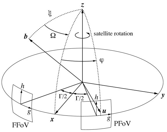
Figure 1: Definition of the instrument axes $\textstyle x$, $\textstyle y$, $\textstyle z$ of the Scanning Reference System (SRS), the basic angle $\Gamma$, and the field angles $g$ and $h$ specifying the observed direction to a star ($\textstyle u$) in either field of view. $\varphi$ is the along-scan instrument angle of the star. In the SRS the direction to the solar system barycentre, $\textstyle b$, is specified by the angles $\xi$ and $\Omega$.

2.3 Variations of the field angles due to a change in the basic angle

Any increase or decrease of the basic angle makes the fields of view move further from each other or closer together. This, in turn, changes the observed field angle $g$ for a given stellar image. However, since the attitude (celestial pointing of the SRS axes) is unchanged, the value of $\varphi$ for a given star is not affected by the basic angle. For example, let us consider the preceding field of view. An increase of the basic angle causes the observed image to be shifted with respect to the centre of the field of view so that the observed along-scan field angle $g_{\mathrm{p}}$ is decreased. The opposite effect takes place in the following field of view. The across-scan field angles $h_{\mathrm{p}}$ and $h_{\mathrm{f}}$ are obviously not affected. The variations of the field angles caused by the basic-angle variation $\delta\Gamma$ are therefore

$$\left.\begin{aligned} \delta g_{\mathrm{p}}&=-{\textstyle\frac{1}{2}}\,\delta\Gamma\\ \delta g_{\mathrm{f}}&=+{\textstyle\frac{1}{2}}\,\delta\Gamma\\ \delta h_{\mathrm{p}}&=0\\ \delta h_{\mathrm{f}}&=0\\ \end{aligned}\quad\right\}\,.$$ (4)

This agrees with Eq. (2) taking into account that $\delta\varphi=0$.

2.4 Variations of the field angles due to a change in the attitude

A quaternion representation is used to parametrise the attitude of Gaia (Lindegren et al., 2012, Appendix A). Here it is more convenient to describe small changes in the attitude by means of three small angles $\delta_{x}$, $\delta_{y}$, and $\delta_{z}$ representing the rotations around the corresponding SRS axes. Since the direction $\textstyle u$ to the star is regarded here as fixed, the corresponding changes in the observed field angles are found to be

$$\left.\begin{aligned} \delta g_{\mathrm{p}}&=-\delta_{z}\\ \delta g_{\mathrm{f}}&=-\delta_{z}\\ \delta h_{\mathrm{p}}&=\cos(\Gamma_{\mathrm{c}}/2)\,\delta_{y}-\sin(\Gamma_{\mathrm{c}}/2)\,\delta_{x}\\ \delta h_{\mathrm{f}}&=\cos(\Gamma_{\mathrm{c}}/2)\,\delta_{y}+\sin(\Gamma_{\mathrm{c}}/2)\,\delta_{x}\end{aligned}\quad\right\}\,.$$ (5)

In these and following equations, we neglect terms of the second and higher orders in $\delta_{x}$, $\delta_{y}$, $\delta_{z}$, and $\delta\Gamma$. To this approximation we can use $\Gamma_{\mathrm{c}}$ instead of $\Gamma$ in the trigonometric factors.

2.5 Combined changes in the basic angle and attitude

Combining Eqs. (4) and (5) we see that a simultaneous change of the basic angle by $\delta\Gamma$ and of the attitude by $\delta_{x}$, $\delta_{y}$, $\delta_{z}$ gives the following total change of the field angles:

$$\left.\begin{aligned} \delta g_{\mathrm{p}}&=-{\textstyle\frac{1}{2}}\,\delta\Gamma-\delta_{z}\\ \delta g_{\mathrm{f}}&=+{\textstyle\frac{1}{2}}\,\delta\Gamma-\delta_{z}\\ \delta h_{\mathrm{p}}&=\cos(\Gamma_{\mathrm{c}}/2)\,\delta_{y}-\sin(\Gamma_{\mathrm{c}}/2)\,\delta_{x}\\ \delta h_{\mathrm{f}}&=\cos(\Gamma_{\mathrm{c}}/2)\,\delta_{y}+\sin(\Gamma_{\mathrm{c}}/2)\,\delta_{x}\end{aligned}\quad\right\}\,.$$ (6)

An exact inversion of this system of equations gives

$$\left.\begin{aligned} \delta_{x}&=\frac{1}{2\sin\left(\Gamma_{\mathrm{c}}/2\right)}\left(\delta h_{\mathrm{f}}-\delta h_{\mathrm{p}}\right)\\ \delta_{y}&=\frac{1}{2\cos(\Gamma_{\mathrm{c}}/2)}\left(\delta h_{\mathrm{p}}+\delta h_{\mathrm{f}}\right)\\ \delta_{z}&=-\frac{1}{2}\left(\delta g_{\mathrm{p}}+\delta g_{\mathrm{f}}\right)\\ \delta\Gamma&=\delta g_{\mathrm{f}}-\delta g_{\mathrm{p}}\end{aligned}\quad\right\}\,.$$ (7)

The first two equations in (7) show that arbitrary small changes in the across-scan field angles $\delta h_{\mathrm{p}}$ and $\delta h_{\mathrm{f}}$ to first order can be represented as changes in the attitude by $\delta_{x}$ and $\delta_{y}$. Similarly, the last two equations show that arbitrary changes in the along-scan field angles $\delta g_{\mathrm{p}}$ and $\delta g_{\mathrm{f}}$ can be represented as a combination of a change of the basic angle $\delta\Gamma$ and a change in the attitude by $\delta_{z}$.

In general, an arbitrary perturbation of the observed stellar positions, being a smooth function of time and stellar position, clearly result in a smooth, time-dependent variation of $\delta g_{\mathrm{p}}$, $\delta g_{\mathrm{f}}$, $\delta h_{\mathrm{p}}$, and $\delta g_{\mathrm{f}}$. From Eq. (7) it follows that such a perturbation is observationally indistinguishable from a certain time-dependent variation of $\delta_{x}$, $\delta_{y}$, $\delta_{z}$, and $\delta\Gamma$.

2.6 Variations of the field angles due to a change in the parallax

The position of the barycentre of the solar system with respect to the instrument can be specified by a distance $R$ (in au) and two angular coordinates. We take the angular coordinates to be $\xi$ and $\Omega$ defined as in Fig. 1. According to the scanning law, $\xi$ is nearly constant while $\Omega$ is increasing with time as the satellite spins. The barycentric position of the satellite is

$$\mathchoice{\mbox{\boldmath$\displaystyle R$}}{\mbox{\boldmath$\textstyle R$}}{\mbox{\boldmath$\scriptstyle R$}}{\mbox{\boldmath$\scriptscriptstyle R$}}=R\left(-\mathchoice{\mbox{\boldmath$\displaystyle x$}}{\mbox{\boldmath$\textstyle x$}}{\mbox{\boldmath$\scriptstyle x$}}{\mbox{\boldmath$\scriptscriptstyle x$}}\cos\Omega\sin\xi+\mathchoice{\mbox{\boldmath$\displaystyle y$}}{\mbox{\boldmath$\textstyle y$}}{\mbox{\boldmath$\scriptstyle y$}}{\mbox{\boldmath$\scriptscriptstyle y$}}\sin\Omega\sin\xi-\mathchoice{\mbox{\boldmath$\displaystyle z$}}{\mbox{\boldmath$\textstyle z$}}{\mbox{\boldmath$\scriptstyle z$}}{\mbox{\boldmath$\scriptscriptstyle z$}}\cos\xi\right)\,.$$ (8)

The observed direction $\textstyle u$ to a star is given by Eq. (4) of Lindegren et al. (2012) as a function of the astrometric parameters of the star. Linearisation yields the change in the direction caused by a small change of the parallax $\delta\varpi$:

$$\delta\mathchoice{\mbox{\boldmath$\displaystyle u$}}{\mbox{\boldmath$\textstyle u$}}{\mbox{\boldmath$\scriptstyle u$}}{\mbox{\boldmath$\scriptscriptstyle u$}}=\mathchoice{\mbox{\boldmath$\displaystyle u$}}{\mbox{\boldmath$\textstyle u$}}{\mbox{\boldmath$\scriptstyle u$}}{\mbox{\boldmath$\scriptscriptstyle u$}}\times\left(\mathchoice{\mbox{\boldmath$\displaystyle u$}}{\mbox{\boldmath$\textstyle u$}}{\mbox{\boldmath$\scriptstyle u$}}{\mbox{\boldmath$\scriptscriptstyle u$}}\times\mathchoice{\mbox{\boldmath$\displaystyle R$}}{\mbox{\boldmath$\textstyle R$}}{\mbox{\boldmath$\scriptstyle R$}}{\mbox{\boldmath$\scriptscriptstyle R$}}\,\delta\varpi\right)\,.$$ (9)

We now assume that the direction to a star is changed only from a change of its parallax, while the basic angle and attitude are kept constant. The fixed basic angle implies $\delta\varphi=\delta g$. The fixed attitude means that $\textstyle x$, $\textstyle y$, and $\textstyle z$ are constant, so that Eq. (1) gives the change in direction

$$\delta\mathchoice{\mbox{\boldmath$\displaystyle u$}}{\mbox{\boldmath$\textstyle u$}}{\mbox{\boldmath$\scriptstyle u$}}{\mbox{\boldmath$\scriptscriptstyle u$}}=\mathchoice{\mbox{\boldmath$\displaystyle v$}}{\mbox{\boldmath$\textstyle v$}}{\mbox{\boldmath$\scriptstyle v$}}{\mbox{\boldmath$\scriptscriptstyle v$}}\cos h\,\delta g+\mathchoice{\mbox{\boldmath$\displaystyle w$}}{\mbox{\boldmath$\textstyle w$}}{\mbox{\boldmath$\scriptstyle w$}}{\mbox{\boldmath$\scriptscriptstyle w$}}\,\delta h\,,$$ (10)

where

$$\left.\begin{aligned} \mathchoice{\mbox{\boldmath$\displaystyle v$}}{\mbox{\boldmath$\textstyle v$}}{\mbox{\boldmath$\scriptstyle v$}}{\mbox{\boldmath$\scriptscriptstyle v$}}&=-\mathchoice{\mbox{\boldmath$\displaystyle x$}}{\mbox{\boldmath$\textstyle x$}}{\mbox{\boldmath$\scriptstyle x$}}{\mbox{\boldmath$\scriptscriptstyle x$}}\sin\varphi+\mathchoice{\mbox{\boldmath$\displaystyle y$}}{\mbox{\boldmath$\textstyle y$}}{\mbox{\boldmath$\scriptstyle y$}}{\mbox{\boldmath$\scriptscriptstyle y$}}\cos\varphi\\ \mathchoice{\mbox{\boldmath$\displaystyle w$}}{\mbox{\boldmath$\textstyle w$}}{\mbox{\boldmath$\scriptstyle w$}}{\mbox{\boldmath$\scriptscriptstyle w$}}&=-\mathchoice{\mbox{\boldmath$\displaystyle x$}}{\mbox{\boldmath$\textstyle x$}}{\mbox{\boldmath$\scriptstyle x$}}{\mbox{\boldmath$\scriptscriptstyle x$}}\cos\varphi\sin h-\mathchoice{\mbox{\boldmath$\displaystyle y$}}{\mbox{\boldmath$\textstyle y$}}{\mbox{\boldmath$\scriptstyle y$}}{\mbox{\boldmath$\scriptscriptstyle y$}}\sin\varphi\sin h+\mathchoice{\mbox{\boldmath$\displaystyle z$}}{\mbox{\boldmath$\textstyle z$}}{\mbox{\boldmath$\scriptstyle z$}}{\mbox{\boldmath$\scriptscriptstyle z$}}\cos h\end{aligned}\quad\right\}$$ (11)

are unit vectors in the directions of increasing $\varphi$ and $h$, respectively. They are evidently orthogonal to each other and to $\textstyle u$. Equating $\delta\mathchoice{\mbox{\boldmath$\displaystyle u$}}{\mbox{\boldmath$\textstyle u$}}{\mbox{\boldmath$\scriptstyle u$}}{\mbox{\boldmath$\scriptscriptstyle u$}}$ from (9) and (10) and taking the dot product with $\textstyle v$ and $\textstyle w$ gives

$$\left.\begin{aligned} \cos h\,\delta g&=-\mathchoice{\mbox{\boldmath$\displaystyle v$}}{\mbox{\boldmath$\textstyle v$}}{\mbox{\boldmath$\scriptstyle v$}}{\mbox{\boldmath$\scriptscriptstyle v$}}^{\prime}\mathchoice{\mbox{\boldmath$\displaystyle R$}}{\mbox{\boldmath$\textstyle R$}}{\mbox{\boldmath$\scriptstyle R$}}{\mbox{\boldmath$\scriptscriptstyle R$}}\,\delta\varpi\\ \delta h&=-\mathchoice{\mbox{\boldmath$\displaystyle w$}}{\mbox{\boldmath$\textstyle w$}}{\mbox{\boldmath$\scriptstyle w$}}{\mbox{\boldmath$\scriptscriptstyle w$}}^{\prime}\mathchoice{\mbox{\boldmath$\displaystyle R$}}{\mbox{\boldmath$\textstyle R$}}{\mbox{\boldmath$\scriptstyle R$}}{\mbox{\boldmath$\scriptscriptstyle R$}}\,\delta\varpi\end{aligned}\quad\right\}\,.$$ (12)

Substituting Eqs. (8) and (11) we find

$$\left.\begin{aligned} \cos h\,\delta g&=-\sin\left(\Omega+\varphi\right)\sin\xi\,R\,\delta\varpi\\ \delta h&=\left[\cos h\cos\xi-\cos(\Omega+\varphi)\sin h\sin\xi\right]\,R\,\delta\varpi\end{aligned}\quad\right\}\,.$$ (13)

Up to this point the derived formulae are valid throughout the field of view to first order in the (very small) variations denoted with a $\delta$. To proceed, we now consider a star observed at the center of either field of view, so that $g=h=0$ and $\varphi=\pm\,\Gamma_{\mathrm{c}}/2$. In this case the variations of the field angles caused by $\delta\varpi$ become

$$\left.\begin{aligned} \delta g_{\mathrm{p}}&=-\sin\left(\Omega+\Gamma_{\mathrm{c}}/2\right)\sin\xi\,R\,\delta\varpi\\ \delta g_{\mathrm{f}}&=-\sin\left(\Omega-\Gamma_{\mathrm{c}}/2\right)\sin\xi\,R\,\delta\varpi\\ \delta h_{\mathrm{p}}&=\cos\xi\,R\,\delta\varpi\\ \delta h_{\mathrm{f}}&=\cos\xi\,R\,\delta\varpi\,.\end{aligned}\quad\right\}\,.$$ (14)

Considering only stars at the centre of either field of view effectively means that we neglect the finite size of the field of view. In both Hipparcos and Gaia the half-size of the field of view is $\Phi<10^{-2}$ rad. Since $|g|$, $|h|<\Phi$, neglected terms in Eq. (14) are of the order of $\Phi\times\delta$, where $\delta$ represents any of the quantities $\delta\Gamma$, $\delta_{x}$, etc. Equation (14) is therefore expected to be accurate to $<1$% at any point in the field of view. The implications of this approximation are further discussed in Sect. 4.4.

2.7 Relation between the changes in parallax, basic angle, and attitude

Substituting Eq. (14) into Eq. (7) we readily obtain a relation between the change in parallax and the corresponding changes in basic angle and attitude:

$$\left.\begin{aligned} \delta_{x}&=0\\ \delta_{y}&=\cos\xi\sec(\Gamma_{\mathrm{c}}/2)\,R\,\delta\varpi\\ \delta_{z}&=\sin\Omega\sin\xi\cos(\Gamma_{\mathrm{c}}/2)\,R\,\delta\varpi\\ \delta\Gamma&=2\cos\Omega\sin\xi\sin(\Gamma_{\mathrm{c}}/2)\,R\,\delta\varpi\end{aligned}\quad\right\}\,.$$ (15)

These equations should be interpreted as follows: a change in parallax by $\delta\varpi$ is observationally indistinguishable (to order $\Phi\times\delta$) from a simultaneous change of the attitude by $\delta_{x}$, $\delta_{y}$, $\delta_{z}$ and of the basic angle by $\delta\Gamma$. The formulae were derived for one star, but if $\delta\varpi$ is the same for all stars, they hold for all observations of all stars. Equation (15) therefore defines the specific variations of the attitude and basic angle that mimic a global shift in parallax. Remarkably, the rotation around the $\textstyle x$ axis is not affected by the global parallax change, while the rotation around the $\textstyle y$ axis is independent of $\Omega$ and therefore, in practice, almost constant.

In a global astrometric solution all the attitude and stellar parameters (including $\varpi$) are simultaneously fitted to the observations of $g$ and $h$. A specific variation in the basic angle of the form $\delta\Gamma(t)\propto\cos\Omega\sin\xi\,R$ will then lead to a global shift of the fitted parallaxes (together with some time-dependent attitude errors $\delta_{y}$, $\delta_{z}$). Since the effects of such a basic-angle variation are fully absorbed by the attitude parameters and parallaxes, the variation is completely degenerate with the stellar and attitude model and cannot be detected from the residuals of the fit.

For a satellite in orbit around the Earth (as Hipparcos) or near L₂ (as Gaia), $R$ is approximately constant. In order to achieve a stable thermal regime of the instrument for a scanning astrometric satellite one typically chooses a scanning law with a constant angle between the direction to the Sun and the spin axis – the so-called solar aspect angle. This means that angle $\xi$ is nearly constant as well (see Sect. 4.5). In the next section we consider the case when $R$ and $\xi$ are exactly constant. Nevertheless, in reality both $R$ and $\xi$ are somewhat time-dependent, and this case is discussed in Sect. 4.3.

Since $\xi$ and $R$ are nearly constant, the degenerate component of the basic-angle variation is essentially of the form $\cos\Omega$, which is periodic with the satellite spin period relative to the solar-system barycentre. This leads to a fundamental design requirement for a scanning astrometry satellite, namely that the basic angle should not have significant periodic variations with a period close to the period of rotation of the satellite, and especially not of the form $\cos\Omega$.

2.8 Harmonic representation of the variations

From Eq. (15) it is seen that a global parallax shift corresponds to variations of $\delta\Gamma$ and $\delta_{z}$ proportional to $\cos\Omega$ and $\sin\Omega$, respectively, while $\delta_{y}$ and $\delta_{x}$ are constant. These quantities correspond to terms of order $k=0$ and 1 in the more general harmonic series

$$\left.\begin{aligned} \delta_{x}&=\sum_{k\geq 0}a_{k}^{(x)}\cos k\Omega+b_{k}^{(x)}\sin k\Omega\\ \delta_{y}&=\sum_{k\geq 0}a_{k}^{(y)}\cos k\Omega+b_{k}^{(y)}\sin k\Omega\\ \delta_{z}&=\sum_{k\geq 0}a_{k}^{(z)}\cos k\Omega+b_{k}^{(z)}\sin k\Omega\\ \delta\Gamma&=\sum_{k\geq 0}a_{k}^{(\Gamma)}\cos k\Omega+b_{k}^{(\Gamma)}\sin k\Omega\\ \end{aligned}\quad\right\}\,.$$ (16)

Specifically, if $a_{k}^{(\Gamma)}=b_{k}^{(\Gamma)}=0$ except for $a_{1}^{(\Gamma)}\neq 0$, we find the following relations between the amplitude of the basic angle variation, the global shift of the parallaxes, and the non-zero harmonics of the attitude errors:

$$\left.\begin{aligned} \delta\varpi&=\frac{1}{2R\sin\xi\sin(\Gamma_{\mathrm{c}}/2)}\,a_{1}^{(\Gamma)}=0.8738\,a_{1}^{(\Gamma)}\\ a_{0}^{(y)}&=\frac{1}{\tan\xi\sin\Gamma_{\mathrm{c}}}\,a_{1}^{(\Gamma)}=1.0429\,a_{1}^{(\Gamma)}\\ b_{1}^{(z)}&=\frac{1}{2\tan(\Gamma_{\mathrm{c}}/2)}\,a_{1}^{(\Gamma)}=0.3734\,a_{1}^{(\Gamma)}\\ \end{aligned}\quad\right\}\,.$$ (17)

The numerical values correspond to the mean parameters relevant for Gaia, that is $\Gamma_{\mathrm{c}}=106\aas@@fstack{\circ}5$, $\xi=45\degr$, and $R=1.01$ au.

It is not the purpose of this paper to investigate the possible effects of other harmonics of the basic-angle variation. However, it can be mentioned that $a_{1}^{(\Gamma)}$ is the only harmonic parameter that is degenerate with the attitude and stellar parameters. This means that $a_{0}^{(\Gamma)}$, $b_{1}^{(\Gamma)}$, and $a_{k}^{(\Gamma)}$, $b_{k}^{(\Gamma)}$ for $k>1$ can be determined as parameters in the calibration model.

3 Results of numerical simulations

In this section we present the results of numerical tests performed to check the above conclusions. To study different aspects of the problem, we make use of two different, though complimentary, solutions: a direct solution, where inversion of the normal matrix provides full covariance information, and an iterative solution, with separate updates for different groups of unknowns, similar to the method used in the actual processing of Gaia data (Lindegren et al., 2012). While the direct solution can only handle a relatively small number of stars, and therefore is of limited practical use, it enables us to investigate important mathematical properties of the problem and to examine the correlations between all the parameters. By contrast, the iterative solution cannot provide this kind of information, but is more realistic in terms of the number of stars and has been successfully employed in the processing of real Gaia data.

3.1 Small-scale direct solutions

For the direct solutions a special simulation software was developed. It simulates the observations of a small number of stars and the reconstruction of their astrometric parameters based on conventional least-squares fitting. The normal equations for the unknown parameters are accumulated and the normal matrix is inverted using singular value decomposition (Golub & van Loan, 1996). This decomposition allows us to study mathematical properties of the problem, especially details of its degeneracy. The simulations included $10^{4}$ stars uniformly distributed over the celestial sphere. Observations were generated with a harmonic perturbation of the basic angle as in Eq. (16d) with $a_{1}^{(\Gamma)}=1$ mas. No noise was added to the observations in order to study the effects of the basic angle variations in pure form. The solutions always include five astrometric parameters per star: two components of the position, the parallax, and two components of the proper motion. Additional parameters representing the variations in attitude and basic angle were introduced as required by various types of solutions.

The first test is to check the theoretical predictions in Eq. (17). To this end, a solution was made including only the star (S) and attitude (A) parameters, where the latter were taken to be the harmonic amplitudes of $\delta_{x}$, $\delta_{y}$, and $\delta_{z}$ as given by the first three equations of (16) for $k\leq 1$, i.e. with a total of nine attitude parameters. The results of this solution, summarised in Table 1, are in very good agreement with the theoretical expectations. Small deviations from the predicted values may be caused e.g. by the limited number of stars, the finite size of the field of view, and numerical rounding errors.

Another test is the singular value analysis of the normal matrix. In addition to the solution described above (of type SA), we computed three other solutions with different sets of unknowns but always using the same observations. Solution S included only the star parameters as unknowns, solution SB included also the harmonic coefficients of $\delta\Gamma$ in the last equation of (16) for $k\leq 1$, and solution SBA included all three sets of unknowns.

The results, summarised in Table 2, again confirm the theoretical predictions. The problem is close to being degenerate only in case SBA where all three kinds of parameters (star, basic angle, attitude) are fitted simultaneously. In this case there is one singular value (${\sim}10^{-5}$) much smaller than the second smallest value (${\sim}10^{-2}$). This indicates that the problem has a rank deficiency of one, which is clearly caused by the (near-)degeneracy between the global parallax shift and the specific basic-angle and attitude variations described by Eq. (17). In all other cases (SB, SA, S) no isolated small singular values appear: the problem is then formally well-conditioned, although (as we have seen in case SA) the solutions may be biased by the basic-angle variations.

Table 1: The parallax shift and the attitude harmonics obtained in the small-scale direct solution (of type SA) with $a_{1}^{(\Gamma)}=1$ mas basic-angle variation.

Quantity	Predicted	Computed
	[mas]	[mas]
$\delta\varpi$	0.8738	0.8735
$a_{0}^{(x)}$	0	$4\times 10^{-6}$
$a_{1}^{(x)}$	0	$9\times 10^{-6}$
$b_{1}^{(x)}$	0	$2\times 10^{-6}$
$a_{0}^{(y)}$	1.0429	1.0423
$a_{1}^{(y)}$	0	$2\times 10^{-5}$
$b_{1}^{(y)}$	0	$-2\times 10^{-6}$
$a_{0}^{(z)}$	0	$-8\times 10^{-6}$
$a_{1}^{(z)}$	0	$-2\times 10^{-5}$
$b_{1}^{(z)}$	0.3734	0.3733

Table 2: The singular values $\sigma_{i}$ of the normal matrix for the different types of direct solutions.

	SBA	SB	SA	S
$\sigma_{1}$	$5.6\times 10^{-6}$	0.015	0.017	0.017
$\sigma_{2}$	0.017	0.017	0.017	0.017
⋮	⋮	⋮	⋮	⋮
$\sigma_{\mathrm{max}}$	1549	387	1549	0.886

The circumstance that the smallest singular value in case SBA is not zero is partly attributable to rounding errors in a solution involving $\geq 50\,000$ unknowns. However, even in exact arithmetics the small-scale direct solution does not represent a fully degenerate problem because (i) the strict degeneracy only occurs if one neglects the finite size of the fields of view, and (ii) some parameters of the mission are slightly time-dependent, but were assumed to be constant by the harmonic representations in Eq. (16). The question of the time dependence is further addressed in Sect. 4.3.

The attitude parameters used in the small-scale solutions are not representative of any practically useful attitude model, but were chosen solely to verify the expected degeneracy with the basic angle variation and parallax zero point. In particular, the harmonic model of $\delta_{x}$, $\delta_{y}$, $\delta_{z}$ in Eq. (16) cannot describe a solid rotation of the reference frame, which explains why Table 2 does not show the six-fold degeneracy between the attitude and stellar parameters normally expected from the unconstrained reference frame. This simplification is removed in the large-scale simulations described below, which use a fully realistic attitude model.

3.2 Large-scale iterative solutions

To test the effect of the basic angle variation in an iterative solution, we make use of the Gaia AGISLab simulation software (Holl et al., 2012, Appendix B). This tool allows us to simulate independent astrometric solutions in a reasonable time, based on the same principles as the astrometric global iterative solution (AGIS; Lindegren et al., 2012) used for Gaia but employing a smaller number of primary stars and several other time-saving simplifications.

To investigate the parallax zero point we have done a set of tests for different values of the basic angle in the range from $30\degr$ to $150\degr$, including the Hipparcos and Gaia values of $58\degr$ and $106\aas@@fstack{\circ}5$, respectively. The nominal Gaia scanning law and realistic geometry of the Gaia fields of view are assumed in these simulations which include one million bright ($G=13$) stars uniformly distributed on the sky and observed during 5 years with no dead time. The nominal along-scan observation noise of 95 $\mu$as per CCD is assumed, based on the estimated centroiding performance of Gaia for stars of $G=13$ mag. According to de Bruijne (2012) this corresponds to an expected end of mission precision of around 10 $\mu$as for the parallaxes. Additionally, basic-angle variations with an amplitude $a_{1}^{\left(\Gamma\right)}=1$ mas are included. The unknowns consist of the five astrometric parameters per star and the attitude parameters based on a B-spline representation of the quaternion components (Lindegren et al., 2012) using a knot interval of 30 s. The AGISLab simulations therefore incorporate many detailed features from the observations and data reductions of an actual scanning astrometric mission, including a number of higher-order effects neglected in our analytical approach.

The parallaxes obtained in the iterative solutions are offset from their ”true” values (assumed in the simulation) by random and systematic errors. Results for the mean offset $\delta\varpi$ are shown by the points in Fig. 2. The curve is the theoretical relation from the first equation in (17). The points deviate from the curve by at most 1 $\mu$as, or $\lesssim 0.1$%. The random errors, measured by the sample standard deviation of the offsets of the individual parallaxes, were 7.3 $\mu$as in all the experiments, practically independent of the basic angle and in rough agreement with the expected end of mission precision.

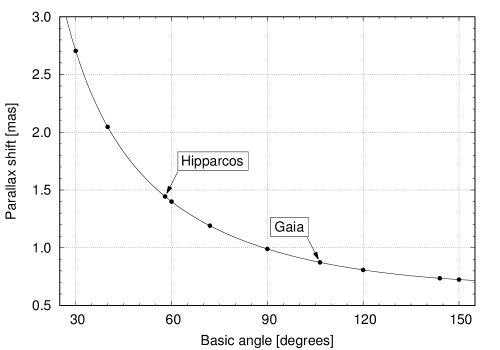
Figure 2: Parallax zero point shift for a basic angle variation of the form $\cos\Omega$ with amplitude 1 mas. The dots show results of the large-scale iterative solution for several different basic angles, including the Hipparcos and Gaia values; the solid curve shows the theoretical relation from Eq. (17).

4 Discussion

In the preceding sections it was shown that a global shift of the parallaxes is observationally indistinguishable from a certain time-variation of the basic angle. The relevant relation, strictly valid at the centre of the field of view, is given by the last identity in Eq. (15). Here we proceed to discuss some practical implications of this result.

4.1 Physical relevance of the cos $\Omega$ dependence

Elementary design principles have led to the choice of a nearly constant solar aspect angle $\xi$ (Fig. 1) for both Hipparcos (43°) and Gaia (45°). Moreover, for a satellite in orbit around the Earth or close to the second Lagrange (L₂) point of the Sun-Earth-Moon system, the barycentric distance $R$ is always close to 1 au. The form of basic-angle variation that is degenerate with parallax is then essentially proportional to $\cos\Omega$. This result is highly significant in relation to expected thermal variations of the instrument. The oblique solar illumination of the rotating satellite may produce basic-angle variations that are periodic with the spin period relative to the Sun, i.e. of the general harmonic form of the last line in Eq. (16). A nearly constant, non-zero coefficient $a_{1}^{(\Gamma)}$ could therefore be a very realistic physical consequence of the way the satellite is operated.

Knowledge of the close coupling between a possible thermal impact on the instrument and the parallax zero point has resulted in very strict engineering specifications for the acceptable amplitude of short-term variations of the basic angle in both Hipparcos and Gaia. In the case of Gaia it was known already at an early design phase that the basic angle variations cannot be fully avoided passively and need to be measured. Therefore Gaia includes a dedicated laser-interferometric metrology system, the basic angle monitor (BAM; Mora et al., 2014), to measure the short-term variations. According to BAM measurements during the first year of the nominal operations of Gaia, the amplitude of the $\cos\Omega$ term, referred to 1.01 au and epoch 2015.0, was about 0.848 mas (Lindegren et al., 2016). Uncorrected, such a large variation would lead to a parallax bias of 0.741 mas according to Eq. (17). For Gaia Data Release 1 (Gaia Collaboration et al., 2016a) the observations were corrected for the basic angle variations based on a harmonic model fitted to the BAM measurements.

4.2 Dependence on $\Gamma_{\mathrm{c}}$

From Eq. (17) it is seen that the parallax shift is inversely proportional to $\sin(\Gamma_{\mathrm{c}}/2)$. For a constant amplitude of the $\cos\Omega$ term in the basic angle variation, the parallax shift therefore decreases with increasing basic angle (cf. Fig. 2). From this point of view the optimum basic angle is therefore 180°. This value would however be very bad for the overall conditioning and precision of the astrometric solution (Makarov, 1997, 1998; Lindegren & Bastian, 2011), which instead favours a value around 90°. Moreover, the sensitivity to the $\cos\Omega$ variation is only a factor 1.4 smaller at 180° than at 90°. The Gaia value $\Gamma_{\mathrm{c}}=106\aas@@fstack{\circ}5$ is therefore a reasonable choice.

That the sensitivity to the basic angle variation increases with decreasing $\Gamma_{\mathrm{c}}$ can be understood from simple arguments. Consider the along-scan effects of the parallax shift $\delta\varpi$. As long as the nominal basic angle $\Gamma_{\mathrm{c}}$ is large, the effects in the two fields of view are significantly different. However, the smaller the basic angle is, the more similar are the effects in the two fields of view. This can be seen from Eq. (14) but is also obvious without any formula. We emphasise that it is the basic angle variations that induce field angle perturbations and that the solution tries to find parallaxes and attitude parameters that fit the perturbed field angles. It is then obvious that a smaller basic angle will require a larger parallax shift to absorb a basic-angle variation of given amplitude.

4.3 Time dependence of $R$ and $\xi$

As noted above, the barycentric distance $R$ and the angle $\xi$ are not strictly constant but functions of time. In this case Eq. (15) gives the particular time dependences of $\delta\Gamma$, $\delta_{x}$, $\delta_{y}$, and $\delta_{z}$ that are degenerate with a global parallax shift. In particular,

$$\delta\Gamma(t)=C\,R(t)\sin\xi(t)\cos\Omega(t)\,,$$ (18)

where $C$ is constant, is indistinguishable from a parallax shift of $\delta\varpi=\frac{1}{2}C/\sin(\Gamma_{\mathrm{c}}/2)$.

Any other form of the variation $\delta\Gamma(t)$ is not completely degenerate with $\delta\varpi$ and may therefore contain components that can be detected by analysis of the residuals and subsequently eliminated by means of additional calibration terms. However, an arbitrary variation $\delta\Gamma(t)$ in general also contains a component of the form (18), which will result in some parallax shift. This shift can be estimated by projecting the variation onto the function on the right-hand side of Eq. (18) in the least-squares sense:

$$\delta\varpi={1\over 2\sin(\Gamma_{\mathrm{c}}/2)}\,{\bigl{\langle}\,\delta\Gamma(t)\,R(t)\,\sin\xi(t)\,\cos\Omega(t)\,\bigr{\rangle}\over\bigl{\langle}\,R(t)^{2}\,\sin^{2}\xi(t)\,\cos^{2}\Omega(t)\,\bigr{\rangle}}\,,$$ (19)

where the angular brackets denote averaging over time. If $R$ and $\xi$ are constant, the factor $(R\sin\xi)^{-1}$ can be taken out of the averages. If, in addition, $\delta\Gamma(t)$ is strictly periodic in $\Omega$, we recover the first equality in Eq. (17).

For Gaia, which operates in the vicinity of L₂, its barycentric distance $R$ varies between approximately 0.99 and 1.03 au as a combination of the eccentric heliocentric orbit of the Earth, the Lissajour orbit around L₂ and the time-dependent offset between the Sun and the Solar system’s barycentre. As discussed in Sect. 4.5 below $\xi$ varies by about 1% from its nominal value 45°.

4.4 Effect of the finite size of the fields of view

In order to derive Eqs. (14) and (15) we neglected the finite size of the field of view by considering only observations at the field centre ($g=h=0$). This was necessary in order to obtain an exact relation between the parallax shift and the basic-angle and attitude variations. In a finite field of view, additional terms appear due to the variation of the parallax factor across the field, which cannot be represented by a unique set of basic-angle variations. These terms are of the order of $\Phi\simeq 10^{-2}$ times smaller than the basic-angle variations, where $\Phi$ is half the size of the field of view. As a consequence, a basic-angle variation of the form (18) is not strictly degenerate with $\delta\varpi$ and the attitude angles when a finite field of view is considered.

However, if the instrument has also periodic optical distortions separately in each field of view that need to be calibrated, the corresponding, more complex calibration model may contribute to the degeneracy and, in worst case, restore complete degeneracy.

4.5 Dependence on heliotropic coordinates

The spherical coordinates $R$, $\xi$, $\Omega$ introduced in Sect. 2.6 define the position of the solar system barycentre in the scanning reference system (SRS). This is what matters for calculating the parallax effect, which depends on the observer’s displacement from the barycentre. On the other hand, the physical relevance of the $\cos\Omega$ modulation is connected with the changing illumination of the satellite by the Sun, which depends on the heliocentric distance $R_{\mathrm{h}}$ and the (heliotropic) angles $\xi_{\mathrm{h}}$, $\Omega_{\mathrm{h}}$ representing the proper direction towards the centre of the Sun at the time of observation. The difference between the heliotropic and barytropic coordinates is at most about 0.01 au and 0.01 rad, respectively. This is small but should be taken into account for an accurate modelling of the basic-angle variations. In this context it can be noted that the expected thermal impact on the satellite scales as $R_{\mathrm{h}}^{-2}$, while the parallax factor scales as $R$. On the other hand, the scanning law is chosen to keep $\xi_{\mathrm{h}}$ as constant as possible, while $\xi$ can vary at the level of 1%. If the basic angle varies as $R_{\mathrm{h}}^{-2}\sin\xi_{\mathrm{h}}\cos\Omega_{\mathrm{h}}$ it is no longer strictly of the form (18). The resulting parallax bias can be estimated by means of Eq. (19).

4.6 Breaking the degeneracy?

If the basic angle varies as a consequence of the changing solar illumination of the rotating satellite we expect to see a parallax bias according to Eq. (19). However, as discussed above, the degeneracy with the parallax zero point is not perfect, and in principle this opens a possibility to calibrate the basic angle variations from the observations. At least three different effects that contribute to breaking the degeneracy could be used: the finite size of the field of view (Sect. 4.4), the time dependence of $R$ due to the eccentricity of the Earth’s orbit (Sect. 4.3), and the difference between the barytropic and heliotropic angles (Sect. 4.5). Unfortunately all three effects only come in at a level of a few per cent of the variation, or less, which makes the result very sensitive to small errors in the calibration model. Moreover, the finite field of view is of little use if we have to calibrate complex periodic variations of optical distortions independently in each field of view. The best chance may be offered by the time variation of $R$, where the ratio of the parallax effect to the illumination strength goes as $R^{3}$ and consequently varies by $\pm 5$% over the year. Thus the hope to break the degeneracy purely from the observations themselves, i.e. based on the self-calibration principle, is rather limited.

5 Conclusions

We have presented an analysis of the effect of basic angle variations on the global shift of parallaxes derived from observations by a scanning astrometric satellite with two fields of view.

The method of small perturbations was used to derive the changes in the four observables (the across- and along-field angles in both fields of view) resulting from perturbations of four instrument parameters (the basic angle and three components of the attitude). Conversely, any given perturbation of the four observables can equally be represented by a specific combination of the instrument parameters. Applying this technique to the perturbations induced by a change in the parallax, we derived the time-dependent variations of the instrument parameters that exactly mimic a global shift of the parallaxes.

These relations confirm previous findings that an uncorrected variation of the basic angle of the form $a_{1}^{(\Gamma)}\cos\Omega$, with $\Omega$ being the barycentric spin phase, leads to a global shift of the parallax zero point of ${\simeq\,}0.87a_{1}^{(\Gamma)}$ for the parameters of the Gaia design. Results of numerical simulations are in complete agreement with the analytical formulae.

In general, periodic variations of the basic angle can be expected from the thermal impact of solar radiation on the spinning satellite (Lindegren, 1977, 2004). Those periodic variations are typically related to the heliotropic spin phase $\Omega_{\mathrm{h}}$, which is close to the barycentric spin phase $\Omega$. If the thermally-induced variations contain a significant component that is proportional to $\cos\Omega_{\mathrm{h}}$, their effect on the observations is practically indistinguishable from a global shift of the parallaxes. Although the degeneracy is not perfect, it is difficult to break except by using of other kinds of data or external information. In the case of Gaia this includes, in particular, direct measurement of the basic angle variations by means of laser metrology (BAM). The use of astrophysical information such as parallaxes of pulsating stars (Windmark et al., 2011; Gould & Kollmeier, 2016) and quasars is vital for verifying the successful determination of the parallax zero point.