Further and stronger analogy between sampling and optimization: Langevin Monte Carlo and gradient descent

Abstract

In this paper, we revisit the recently established theoretical guarantees for the convergence of the Langevin Monte Carlo algorithm of sampling from a smooth and (strongly) log-concave density. We improve the existing results when the convergence is measured in the Wasserstein distance and provide further insights on the very tight relations between, on the one hand, the Langevin Monte Carlo for sampling and, on the other hand, the gradient descent for optimization. Finally, we also establish guarantees for the convergence of a version of the Langevin Monte Carlo algorithm that is based on noisy evaluations of the gradient.

1 Introduction

Let $p$ be a positive integer and $f:\mathbb{R}^{p}\to\mathbb{R}$ be a measurable function such that the integral $\int_{\mathbb{R}^{p}}\exp\{-f(\boldsymbol{\theta})\}\,d\boldsymbol{\theta}$ is finite. In various applications, one is faced with the problems of finding the minimum point of $f$ or computing the average with respect to the probability density

$$\pi(\boldsymbol{\theta})=\frac{e^{-f(\boldsymbol{\theta})}}{\int_{\mathbb{R}^{p}}e^{-f(\boldsymbol{u})}\,d\boldsymbol{u}}.$$ (1)

In other words, one often looks for approximating the values $\boldsymbol{\theta}^{*}$ and $\bar{\boldsymbol{\theta}}$ defined as

$$\bar{\boldsymbol{\theta}}=\int_{\mathbb{R}^{p}}\boldsymbol{\theta}\,\pi(\boldsymbol{\theta})\,d\boldsymbol{\theta},\qquad\boldsymbol{\theta}^{*}\in\text{arg}\min_{\boldsymbol{\theta}\in\mathbb{R}^{p}}f(\boldsymbol{\theta}).$$ (2)

In most situations, the approximations of these values are computed using iterative algorithms which share many common features. There is a vast variety of such algorithms for solving both tasks, see for example (Boyd and Vandenberghe, 2004) for optimization and (Atchadé et al., 2011) for approximate sampling. The similarities between the task of optimization and that of averaging have been recently exploited in the papers (Dalalyan, 2014; Durmus and Moulines, 2016; Durmus et al., 2016) in order to establish fast and accurate theoretical guarantees for sampling from and averaging with respect to the density $\pi$ using the Langevin Monte Carlo algorithm. The goal of the present work is to push further this study both by improving the existing bounds and by extending them in some directions.

We will focus on strongly convex functions $f$ having a Lipschitz continuous gradient. That is, we assume that there exist two positive constants $m$ and $M$ such that

$$\begin{cases}f(\boldsymbol{\theta})-f(\boldsymbol{\theta}^{\prime})-\nabla f(\boldsymbol{\theta}^{\prime})^{\top}(\boldsymbol{\theta}-\boldsymbol{\theta}^{\prime})\geq(\nicefrac{{m}}{{2}})\|\boldsymbol{\theta}-\boldsymbol{\theta}^{\prime}\|_{2}^{2},\text{\vphantom{$I_{\textstyle\int_{I_{I}}}$}}\\ \|\nabla f(\boldsymbol{\theta})-\nabla f(\boldsymbol{\theta}^{\prime})\|_{2}\leq M\|\boldsymbol{\theta}-\boldsymbol{\theta}^{\prime}\|_{2},\end{cases}\qquad\forall\boldsymbol{\theta},\boldsymbol{\theta}^{\prime}\in\mathbb{R}^{p},$$ (3)

where $\nabla f$ stands for the gradient of $f$ and $\|\cdot\|_{2}$ is the Euclidean norm. We say that the density $\pi(\boldsymbol{\theta})\propto e^{-f(\boldsymbol{\theta})}$ is log-concave (resp. strongly log-concave) if the function $f$ satisfies the first inequality of (3) with $m=0$ (resp. $m>0$).

The Langevin Monte Carlo (LMC) algorithm studied throughout this work is the analogue of the gradient descent algorithm for optimization. Starting from an initial point $\boldsymbol{\vartheta}^{(0)}\in\mathbb{R}^{p}$ that may be deterministic or random, the iterations of the algorithm are defined by the update rule

$$\boldsymbol{\vartheta}^{(k+1,h)}=\boldsymbol{\vartheta}^{(k,h)}-h\nabla f(\boldsymbol{\vartheta}^{(k,h)})+\sqrt{2h}\;\boldsymbol{\xi}^{(k+1)};\qquad k=0,1,2,\ldots$$ (4)

where $h>0$ is a tuning parameter, referred to as the step-size, and $\boldsymbol{\xi}^{(1)},\ldots,\boldsymbol{\xi}^{(k)},\ldots$ is a sequence of mutually independent, and independent of $\boldsymbol{\vartheta}^{(0)}$, centered Gaussian vectors with covariance matrices equal to identity. Under the assumptions imposed on $f$, when $h$ is small and $k$ is large (so that the product $kh$ is large), the distribution of $\boldsymbol{\vartheta}^{(k,h)}$ is close in various metrics to the distribution with density $\pi(\boldsymbol{\theta})$, hereafter referred to as the target distribution. An important question is to quantify this closeness; this might be particularly useful for deriving a stopping rule for the LMC algorithm.

The measure of approximation used in this paper is the Wasserstein-Monge-Kantorovich distance $W_{2}$. For two measures $\mu$ and $\nu$ defined on $(\mathbb{R}^{p},\mathscr{B}(\mathbb{R}^{p}))$, $W_{2}$ is defined by

$$W_{2}(\mu,\nu)=\Big{(}\inf_{\gamma\in\Gamma(\mu,\nu)}\int_{\mathbb{R}^{p}\times\mathbb{R}^{p}}\|\boldsymbol{\theta}-\boldsymbol{\theta}^{\prime}\|_{2}^{2}\,d\gamma(\boldsymbol{\theta},\boldsymbol{\theta}^{\prime})\Big{)}^{1/2},$$ (5)

where the $\inf$ is with respect to all joint distributions $\gamma$ having $\mu$ and $\nu$ as marginal distributions. This distance is perhaps more suitable for quantifying the quality of approximate sampling schemes than other metrics such as the total variation. Indeed, on the one hand, bounds on the Wasserstein distance—unlike the bounds on the total-variation distance—directly provide the level of approximating the first order moment. For instance, if $\mu$ and $\nu$ are two Dirac measures at the points $\boldsymbol{\theta}$ and $\boldsymbol{\theta}^{\prime}$, respectively, then the total-variation distance $D_{\rm TV}(\delta_{\boldsymbol{\theta}},\delta_{\boldsymbol{\theta}^{\prime}})$ equals one whenever $\boldsymbol{\theta}\not=\boldsymbol{\theta}^{\prime}$, whereas $W_{2}(\delta_{\boldsymbol{\theta}},\delta_{\boldsymbol{\theta}^{\prime}})=\|\boldsymbol{\theta}-\boldsymbol{\theta}^{\prime}\|_{2}$ is a smoothly increasing function of the Euclidean distance between $\boldsymbol{\theta}$ and $\boldsymbol{\theta}^{\prime}$. This seems to better correspond to the intuition on the closeness of two distributions.

2 Improved guarantees for the Wasserstein distance

The rationale behind the LMC algorithm (4) is simple: the Markov chain $\{\boldsymbol{\vartheta}^{(k,h)}\}_{k\in\mathbb{N}}$ is the Euler discretization of a continuous-time diffusion process $\{\boldsymbol{L}_{t}:t\in\mathbb{R}_{+}\}$, known as Langevin diffusion, that has $\pi$ as invariant density (Bhattacharya, 1978, Thm. 3.5). The Langevin diffusion is defined by the stochastic differential equation

$$d\boldsymbol{L}_{t}=-\nabla f(\boldsymbol{L}_{t})\,dt+\sqrt{2}\;d\boldsymbol{W}_{t},\qquad t\geq 0,$$ (6)

where $\{\boldsymbol{W}_{t}:t\geq 0\}$ is a $p$-dimensional Brownian motion. When $f$ satisfies condition (3), equation (6) has a unique strong solution which is a Markov process. Let $\nu_{k}$ be the distribution of the $k$-th iterate of the LMC algorithm, that is $\vartheta^{(k,h)}\sim\nu_{k}$.

Theorem 2.1.

Assume that $h\in(0,\nicefrac{{2}}{{M}})$. The following claims hold:

1. If $h\leq\nicefrac{{2}}{{(m+M)}}$ then $W_{2}(\nu_{K},\pi)\leq(1-mh)^{K}W_{2}(\nu_{0},\pi)+1.82(M/m)(hp)^{1/2}$.

2. If $h\geq\nicefrac{{2}}{{(m+M)}}$ then $W_{2}(\nu_{K},\pi)\leq\displaystyle(Mh-1)^{K}W_{2}(\nu_{0},\pi)+1.82\frac{Mh}{2-Mh}(hp)^{1/2}$.

The proof of this theorem is postponed to Section 6. We content ourselves here by discussing the relation of this result to previous work. Note that if the initial value $\boldsymbol{\vartheta}^{(0)}=\boldsymbol{\theta}^{(0)}$ is deterministic then, according to (Durmus and Moulines, 2016, Theorem 1), we have

$$W_{2}(\nu_{0},\pi)^{2} =\int_{\mathbb{R}^{p}}\|\boldsymbol{\theta}^{(0)}-\boldsymbol{\theta}\|_{2}^{2}\pi(d\boldsymbol{\theta})$$ (7)

$$=\|\boldsymbol{\theta}^{(0)}-\bar{\boldsymbol{\theta}}\|_{2}^{2}+\int_{\mathbb{R}^{p}}\|\bar{\boldsymbol{\theta}}-\boldsymbol{\theta}\|_{2}^{2}\pi(d\boldsymbol{\theta})$$ (8)

$$\leq\|\boldsymbol{\theta}^{(0)}-\bar{\boldsymbol{\theta}}\|_{2}^{2}+p/m.$$ (9)

First of all, let us remark that if we choose $h$ and $K$ so that

$$h\leq\nicefrac{{2}}{{(m+M)}},\qquad e^{-mhK}W_{2}(\nu_{0},\pi)\leq\varepsilon/2,\quad 1.82(M/m)(hp)^{1/2}\leq\varepsilon/2,$$ (10)

then we have $W_{2}(\nu_{K},\pi)\leq\varepsilon$. In other words, conditions (10) are sufficient for the density of the output of the LMC algorithm with $K$ iterations to be within the precision $\varepsilon$ of the target density when the precision is measured using the Wasserstein distance. This readily yields

$$h\leq\frac{m^{2}\varepsilon^{2}}{14M^{2}p}\wedge\frac{2}{m+M}\quad\text{and}\quad hK\geq\frac{1}{m}\log\Big{(}\frac{2(\|\boldsymbol{\theta}^{(0)}-\bar{\boldsymbol{\theta}}\|_{2}^{2}+p/m)^{1/2}}{\varepsilon}\Big{)}$$ (11)

Assuming $m,M$ and $\|\boldsymbol{\theta}^{(0)}-\bar{\boldsymbol{\theta}}\|_{2}^{2}/p$ to be constants, we can deduce from the last display that it suffices $K=Cp\varepsilon^{-2}\log(p/\varepsilon)$ number of iterations in order to reach the precision level $\varepsilon$. This fact has been first established in (Dalalyan, 2014) for the LMC algorithm with a warm start and the total-variation distance. It was later improved by Durmus and Moulines (2016), who showed that the same result holds for any starting point and established similar bounds for the Wasserstein distance.

In order to make the comparison easier, let us recall below the corresponding result from (Durmus and Moulines, 2016). It asserts that under condition (3), if $h\leq\nicefrac{{2}}{{(m+M)}}$ then

$$W_{2}^{2}(\nu_{K},\pi)\leq 2\Big{(}1-\frac{mMh}{m+M}\Big{)}^{K}W^{2}_{2}(\nu,\pi)+\frac{Mhp}{m}(m+M)\Big{(}h+\frac{m+M}{2mM}\Big{)}\Big{(}2+\frac{M^{2}h}{m}+\frac{M^{2}h^{2}}{6}\Big{)}.$$ (12)

When we compare this inequality with the claims of Theorem 2.1, we see that

1. Theorem 2.1 holds under weaker conditions: $h\leq\nicefrac{{2}}{{M}}$ instead of $h\leq\nicefrac{{2}}{{(m+M)}}$.

2. The analytical expressions of the upper bounds on the Wasserstein distance in Theorem 2.1 are not as involved as those of (12).

3. If we take a closer look, we can check that when $h\leq\nicefrac{{2}}{{(m+M)}}$, the upper bound in part (a) of Theorem 2.1 is sharper than that of (12).

In order to better illustrate the claim in iii) above, we consider a numerical example in which $m=4$, $M=5$ and $\|\boldsymbol{\theta}^{(0)}-\bar{\boldsymbol{\theta}}\|_{2}^{2}=p$. Let $F_{\rm our}(h,K,p)$ and $F_{\rm DM}(h,K,p)$ be the upper bounds on $W_{2}(\nu_{K},\pi)$ provided by Theorem 2.1 and (12). For different values of $p$, we compute

$$K_{\rm our}(p) =\min\big{\{}K:\text{ there exists $h\leq\nicefrac{{2}}{{(m+M)}}$ such that }F_{\rm our}(h,K,p)\leq\varepsilon\big{\}},$$ (13)

$$K_{\rm DM}(p) =\min\big{\{}K:\text{ there exists $h\leq\nicefrac{{2}}{{(m+M)}}$ such that }F_{\rm DM}(h,K,p)\leq\varepsilon\big{\}}.$$ (14)

The curves of the functions $p\mapsto\log K_{\rm our}(p)$ and $p\mapsto\log K_{\rm DM}(p)$, for $\varepsilon=0.1$ and $\varepsilon=0.3$ are plotted in Figure 1. We can deduce from these plots that the number of iterations yielded by our bound is more than 5 times smaller than the number of iterations recommended by bound (12) of Durmus and Moulines (2016).

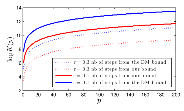
Figure 1: The curves of the functions $p\mapsto\log K(p)$, where $K(p)$ is the number of steps— derived either from our bound or from the bound (12) of (Durmus and Moulines, 2016)—sufficing for reaching the precision level $\varepsilon$ (for $\varepsilon=0.1$ and $\varepsilon=0.3$).

Remark 2.2.

Although the upper bound on $W_{2}(\nu_{0},\pi)$ provided by (9) is relevant for understanding the order of magnitude of $W_{2}(\nu_{0},\pi)$, it has limited applicability since the distance $\|\boldsymbol{\theta}_{0}-\bar{\boldsymbol{\theta}}\|$ might be hard to evaluate. An attractive alternative to that bound is the following:

$$W_{2}(\nu_{0},\pi)^{2} =\int_{\mathbb{R}^{p}}\|\boldsymbol{\theta}^{(0)}-\boldsymbol{\theta}\|_{2}^{2}\pi(d\boldsymbol{\theta})$$ (15)

$$\leq\frac{2}{m}\int_{\mathbb{R}^{p}}\Big{(}f(\boldsymbol{\theta}_{0})-f(\boldsymbol{\theta})-\nabla f(\boldsymbol{\theta})^{\top}(\boldsymbol{\theta}_{0}-\boldsymbol{\theta})\Big{)}\pi(d\boldsymbol{\theta})$$ (16)

$$=\frac{2}{m}\Big{(}f(\boldsymbol{\theta}_{0})-\int_{\mathbb{R}^{p}}f(\boldsymbol{\theta})\,\pi(d\boldsymbol{\theta})+p\Big{)}.$$ (17)

If $f$ is lower bounded by some known constant, for instance if $f\geq 0$, the last inequality provides the computable upper bound $W_{2}(\nu_{0},\pi)^{2}\leq\frac{2}{m}\big{(}f(\boldsymbol{\theta}_{0})+p\big{)}$.

3 Relation with optimization

We have already mentioned that the LMC algorithm is very close to the gradient descent algorithm for computing the minimum $\boldsymbol{\theta}^{*}$ of the function $f$. However, when we compare the guarantees of Theorem 2.1 with those available for the optimization problem, we remark the following striking difference. The approximate computation of $\boldsymbol{\theta}^{*}$ requires a number of steps of the order of $\log(1/\varepsilon)$ to reach the precision $\varepsilon$, whereas, for reaching the same precision in sampling from $\pi$, the LMC algorithm needs a number of iterations proportional to $(p/\varepsilon^{2})\log(p/\varepsilon)$. The goal of this section is to explain that this, at first sight very disappointing behavior of the LMC algorithm is, in fact, continuously connected to the exponential convergence of the gradient descent.

The main ingredient for the explanation is that the function $f(\boldsymbol{\theta})$ and the function $f_{\tau}(\boldsymbol{\theta})=f(\boldsymbol{\theta})/\tau$ have the same point of minimum $\boldsymbol{\theta}^{*}$, whatever the real number $\tau>0$. In addition, if we define the density function $\pi_{\tau}(\boldsymbol{\theta})\propto\exp\big{(}-f_{\tau}(\boldsymbol{\theta})\big{)}$, then the average value

$$\bar{\boldsymbol{\theta}}_{\tau}=\int_{\mathbb{R}^{p}}\boldsymbol{\theta}\,\pi_{\tau}(\boldsymbol{\theta})\,d\boldsymbol{\theta}$$

tends to the minimum point $\boldsymbol{\theta}^{*}$ when $\tau$ goes to zero. Furthermore, the distribution $\pi_{\tau}(d\boldsymbol{\theta})$ tends to the Dirac measure at $\boldsymbol{\theta}^{*}$. Clearly, $f_{\tau}$ satisfies (3) with the constants $m_{\tau}=m/\tau$ and $M_{\tau}=M/\tau$. Therefore, on the one hand, we can apply to $\pi_{\tau}$ claim (a) of Theorem 2.1, which tells us that if we choose $h=1/M_{\tau}=\tau/M$, then

$$W_{2}(\nu_{K},\pi_{\tau})\leq\Big{(}1-\frac{m}{M}\Big{)}^{K}W_{2}(\delta_{\boldsymbol{\theta}^{(0)}},\pi_{\tau})+2\Big{(}\frac{M}{m}\Big{)}\Big{(}\frac{p\tau}{M}\Big{)}^{1/2}.$$ (18)

On the other hand, the LMC algorithm with the step-size $h=\tau/M$ applied to $f_{\tau}$ reads as

$$\boldsymbol{\vartheta}^{(k+1,h)}=\boldsymbol{\vartheta}^{(k,h)}-\frac{1}{M}\nabla f(\boldsymbol{\vartheta}^{(k,h)})+\sqrt{\frac{2\tau}{M}}\;\boldsymbol{\xi}^{(k+1)};\qquad k=0,1,2,\ldots$$ (19)

When the parameter $\tau$ goes to zero, the LMC sequence (19) tends to the gradient descent sequence $\boldsymbol{\theta}^{(k)}$. Therefore, the limiting case of (18) corresponding to $\tau\to 0$ writes as

$$\|\boldsymbol{\theta}^{(K)}-\boldsymbol{\theta}^{*}\|_{2}\leq\Big{(}1-\frac{m}{M}\Big{)}^{K}\|\boldsymbol{\theta}^{(0)}-\boldsymbol{\theta}^{*}\|_{2},$$ (20)

which is a well-known result in Optimization. This clearly shows that Theorem 2.1 is a natural extension of the results of convergence from optimization to sampling.

4 Guarantees for the noisy gradient version

In some situations, the precise evaluation of the gradient $\nabla f(\boldsymbol{\theta})$ is computationally expensive or practically impossible, but it is possible to obtain noisy evaluations of $\nabla f$ at any point. This is the setting considered in the present section. More precisely, we assume that at any point $\boldsymbol{\vartheta}^{(k,h)}\in\mathbb{R}^{p}$ of the LMC algorithm, we can observe the value

$$\boldsymbol{Y}^{(k,h)}=\nabla f(\boldsymbol{\vartheta}^{(k,h)})+\sigma\,\boldsymbol{\zeta}^{(k)},$$ (21)

where $\{\boldsymbol{\zeta}^{(k)}:\,k=0,1,\ldots\}$ is a sequence of independent zero mean random vectors such that $\mathbf{E}[\|\boldsymbol{\zeta}^{(k)}\|_{2}^{2}]\leq p$ and $\sigma>0$ is a deterministic noise level. Furthermore, the noise vector $\boldsymbol{\zeta}^{(k)}$ is independent of the past states $\boldsymbol{\vartheta}^{(1,h)},\ldots,\boldsymbol{\vartheta}^{(k,h)}$. The noisy LMC (nLMC) algorithm is then defined as

$$\boldsymbol{\vartheta}^{(k+1,h)}=\boldsymbol{\vartheta}^{(k,h)}-h\boldsymbol{Y}^{(k,h)}+\sqrt{2h}\;\boldsymbol{\xi}^{(k+1)};\qquad k=0,1,2,\ldots$$ (22)

where $h>0$ and $\boldsymbol{\xi}^{(k+1)}$ are as in (4). The next theorem extends the guarantees of Theorem 2.1 to the noisy-gradient setting and to the nLMC algorithm.

Theorem 4.1.

Let $\boldsymbol{\vartheta}^{(K,h)}$ be the $K$-th iterate of the nLMC algorithm (22) and $\nu_{K}$ be its distribution. If the function $f$ satisfies condition (3) and $h\leq 2/M$ then the following claims hold:

1. If $h\leq\nicefrac{{2}}{{(m+M)}}$ then

   $$W_{2}(\nu_{K},\pi)\leq\Big{(}1-\frac{mh}{2}\Big{)}^{K}W_{2}(\nu_{0},\pi)+\Big{(}\frac{2hp}{m}\Big{)}^{1/2}\Big{\{}\sigma^{2}+\frac{3.3M^{2}}{m}\Big{\}}^{1/2}.$$ (23)

2. If $h\geq\nicefrac{{2}}{{(m+M)}}$ then

   $$W_{2}(\nu_{K},\pi)\leq\Big{(}\frac{Mh}{2}\Big{)}^{K}W_{2}(\nu_{0},\pi)+\Big{(}\frac{2h^{2}p}{2-Mh}\Big{)}^{1/2}\Big{\{}\sigma^{2}+\frac{6.6M}{2-Mh}\Big{\}}^{1/2}.$$

To understand the potential scope of applicability of this result, let us consider a typical statistical problem in which $f(\boldsymbol{\theta})$ is the negative log-likelihood of $n$ independent random variables $X_{1},\ldots,X_{n}$. Then, if $\ell(\boldsymbol{\theta},x)$ is the log-likelihood of one variable, we have

$$f(\boldsymbol{\theta})=\sum_{i=1}^{n}\ell(\boldsymbol{\theta},X_{i}).$$

In such a situation, if the Fisher information is not degenerated, both $m$ and $M$ are proportional to the sample size $n$. When the gradient of $\ell(\boldsymbol{\theta},X_{i})$ with respect to parameter $\boldsymbol{\theta}$ is hard to compute, one can replace the evaluation of $\nabla f(\boldsymbol{\vartheta}^{(k,h)})$ at each step $k$ by that of $Y_{k}=n\nabla_{\boldsymbol{\theta}}\ell(\boldsymbol{\vartheta}^{(k,h)},X_{k})$. Under suitable assumptions, this random vector satisfies the conditions of Theorem 4.1 with a $\sigma^{2}$ proportional to $n$. Therefore, if we analyze the expression between curly brackets in (23), we see that the additional term, $\sigma^{2}$, due to the subsampling is of the same order of magnitude as the term $3.3M^{2}/m$. Thus, using the subsampled gradient in the LMC algorithm does not cause a significant deterioration of the precision while reducing considerably the computational burden.

5 Discussion and outlook

We have established simple guarantees for the convergence of the Langevin Monte Carlo algorithm under the Wasserstein metric. These guarantees are valid under strong convexity and Lipschitz-gradient assumptions on the log-density function, for a step-size smaller than $2/M$, where $M$ is the constant in the Lipschitz condition. These guarantees are sharper than previously established analogous results and in perfect agreement with the analogous results in Optimization. Furthermore, we have shown that similar results can be obtained in the case where only noisy evaluations of the gradient are possible.

There are a number of interesting directions in which this work can be extended. One relevant and closely related problem is the approximate computation of the volume of a convex body, or, the problem of sampling from the uniform distribution on a convex body. This problem has been analyzed by other Monte Carlo methods such as “Hit and Run” in a series of papers by Lovász and Vempala (2006b, a), see also the more recent paper (Bubeck et al., 2015). Numerical experiments reported in (Bubeck et al., 2015) suggest that the LMC algorithm might perform better in practice than “Hit and Run”. It would be interesting to have a theoretical result corroborating this observation.

Other interesting avenues for future research include the possible adaptation of the Nesterov acceleration to the problem of sampling, extensions to second-order methods as well as the alleviation of the strong-convexity assumptions. We also plan to investigate in more depth the applications is high-dimensional statistics (see, for instance, Dalalyan and Tsybakov (2012)). Some results in these directions are already obtained in (Dalalyan, 2014; Durmus and Moulines, 2016; Durmus et al., 2016). It is a stimulating question whether we can combine ideas of the present work and the aforementioned earlier results to get improved guarantees.

6 Proofs

The first part of the proofs of Theorem 2.1 and Theorem 4.1 is the same. We start this section by this common part and then we proceed with the proofs of the two theorems separately.

Let $\boldsymbol{W}$ be a $p$-dimensional Brownian Motion such that $\boldsymbol{W}_{(k+1)h}-\boldsymbol{W}_{kh}=\sqrt{h}\,\boldsymbol{\xi}^{(k+1)}$. We define the stochastic process $\boldsymbol{L}$ so that $\boldsymbol{L}_{0}\sim\pi$ and

$$\boldsymbol{L}_{t} =\boldsymbol{L}_{0}-\int_{0}^{t}\nabla f(\boldsymbol{L}_{s})\,ds+\sqrt{2}\,\boldsymbol{W}_{t},\qquad\forall\,t>0.$$ (24)

It is clear that this equation implies that

$$\displaystyle\boldsymbol{L}_{(k+1)h} =\boldsymbol{L}_{kh}-\int_{kh}^{(k+1)h}\nabla f(\boldsymbol{L}_{s})\,ds+\sqrt{2}\,(\boldsymbol{W}_{(k+1)h}-\boldsymbol{W}_{kh})$$ (25)

$$=\boldsymbol{L}_{kh}-\int_{kh}^{(k+1)h}\nabla f(\boldsymbol{L}_{s})\,ds+\sqrt{2h}\,\boldsymbol{\xi}^{(k+1)}.$$ (26)

Furthermore, $\{\boldsymbol{L}_{t}:t\geq 0\}$ is a diffusion process having $\pi$ as the stationary distribution. Since the initial value $\boldsymbol{L}_{0}$ is drawn from $\pi$, we have $\boldsymbol{L}_{t}\sim\pi$ for every $t\geq 0$.

Let us denote $\boldsymbol{\Delta}_{k}=\boldsymbol{L}_{kh}-\boldsymbol{\vartheta}^{(k,h)}$ and $I_{k}=(kh,(k+1)h]$. We have

$$\boldsymbol{\Delta}_{k+1} =\boldsymbol{\Delta}_{k}+h\boldsymbol{Y}^{(k,h)}-\int_{I_{k}}\nabla f(\boldsymbol{L}_{t})\,dt$$ (27)

$$=\boldsymbol{\Delta}_{k}-h\big{(}\underbrace{\nabla f(\boldsymbol{\vartheta}^{(k,h)}+\boldsymbol{\Delta}_{k})-\nabla f(\boldsymbol{\vartheta}^{(k,h)})}_{:=\boldsymbol{U}_{k}}\big{)}+\sigma h\boldsymbol{\zeta}^{(k)}-\underbrace{\int_{I_{k}}\big{(}\nabla f(\boldsymbol{L}_{t})-\nabla f(\boldsymbol{L}_{kh})\big{)}\,dt}_{:=\boldsymbol{V}_{k}}.$$ (28)

In view of the triangle inequality, we get

$$\|\boldsymbol{\Delta}_{k+1}\|_{2}\leq\|\boldsymbol{\Delta}_{k}-h\boldsymbol{U}_{k}+\sigma h\boldsymbol{\zeta}^{(k)}\|_{2}+\|\boldsymbol{V}_{k}\|_{2}.$$ (29)

For the first norm in the right hand side, we can use the following inequalities:

$$\mathbf{E}[\|\boldsymbol{\Delta}_{k}-h\boldsymbol{U}_{k}+\sigma h\boldsymbol{\zeta}^{(k)}\|_{2}^{2}] =\mathbf{E}[\|\boldsymbol{\Delta}_{k}-h\boldsymbol{U}_{k}\|_{2}^{2}]+\mathbf{E}[\|\sigma h\boldsymbol{\zeta}^{(k)}\|_{2}^{2}]$$ (30)

$$=\mathbf{E}[\|\boldsymbol{\Delta}_{k}-h\boldsymbol{U}_{k}\|_{2}^{2}]+\sigma^{2}h^{2}p.$$ (31)

We need now three technical lemmas the proofs of which are postponed to Section 6.3.

Lemma 1.

Let us introduce the constant $\gamma$ that equals $|1-mh|$ if $h\leq\nicefrac{{2}}{{(m+M)}}$ and $|1-Mh|$ if $h\geq\nicefrac{{2}}{{(m+M)}}$. (Since $h\in(0,\nicefrac{{2}}{{M}})$, this value $\gamma$ satisfies $0<\gamma<1$). It holds that

$$\|\boldsymbol{\Delta}_{k}-h\boldsymbol{U}_{k}\|_{2} \leq\gamma\|\boldsymbol{\Delta}_{k}\|_{2}.$$ (32)

Lemma 2.

If the function $f$ is continuously differentiable and the gradient of $f$ is Lipschitz with constant $M$, then

$$\int_{\mathbb{R}^{p}}\|\nabla f(\boldsymbol{x})\|_{2}^{2}\,\pi(\boldsymbol{x})\,d\boldsymbol{x}\leq Mp.$$ (33)

Lemma 3.

If the function $f$ has a Lipschitz-continuous gradient with the Lipschitz constant $M$, $\boldsymbol{L}$ is the Langevin diffusion (24) and $\boldsymbol{V}(a)=\int_{a}^{a+h}\big{(}\nabla f(\boldsymbol{L}_{t})-\nabla f(\boldsymbol{L}_{a})\big{)}\,dt$ for some $a\geq 0$, then

$$\big{(}\mathbf{E}[\|\boldsymbol{V}(a)\|^{2}_{2}]\big{)}^{1/2} \leq\bigg{(}\frac{1}{3}h^{4}M^{3}p\bigg{)}^{1/2}+(h^{3}p)^{1/2}M.$$ (34)

This completes the common part of the proof. We present below the proofs of the theorems.

6.1 Proof of Theorem 2.1

Using (29) with $\sigma=0$ and 1, we get

$$\|\boldsymbol{\Delta}_{k+1}\|_{2}\leq\gamma\|\boldsymbol{\Delta}_{k}\|_{2}+\|\boldsymbol{V}_{k}\|_{2},\qquad\forall k\in\mathbb{N}.$$ (35)

In view of the Minkowski inequality and 3, this yields

$$(\mathbf{E}[\|\boldsymbol{\Delta}_{k+1}\|_{2}^{2}])^{1/2} \leq\gamma(\mathbf{E}[\|\boldsymbol{\Delta}_{k}\|_{2}^{2}])^{1/2}+(\mathbf{E}[\|\boldsymbol{V}_{k}\|_{2}^{2}])^{1/2}$$ (36)

$$\leq\gamma(\mathbf{E}[\|\boldsymbol{\Delta}_{k}\|_{2}^{2}])^{1/2}+1.82(h^{3}M^{2}p)^{1/2},$$ (37)

where we have used the fact that $h\leq 2/M$. Using this inequality iteratively with $k-1,\ldots,0$ instead of $k$, we get

$$(\mathbf{E}[\|\boldsymbol{\Delta}_{k+1}\|_{2}^{2}])^{1/2} \leq\gamma^{k+1}(\mathbf{E}[\|\boldsymbol{\Delta}_{0}\|_{2}^{2}])^{1/2}+1.82(h^{3}M^{2}p)^{1/2}\sum_{j=0}^{k}\gamma^{j}$$ (38)

$$\leq\gamma^{k+1}(\mathbf{E}[\|\boldsymbol{\Delta}_{0}\|_{2}^{2}])^{1/2}+1.82(h^{3}M^{2}p)^{1/2}(1-\gamma)^{-1}.$$ (39)

Since $\boldsymbol{\Delta}_{k+1}=\boldsymbol{L}_{(k+1)h}-\boldsymbol{\vartheta}^{(k+1,h)}$ and $\boldsymbol{L}_{(k+1)h}\sim\pi$, we readily get the inequality $W_{2}(\nu_{k+1},\pi)\leq\big{(}\mathbf{E}[\|\boldsymbol{\Delta}_{k+1}\|^{2}_{2}]\big{)}^{1/2}$. In addition, one can choose $\boldsymbol{L}_{0}$ so that $W_{2}(\nu_{0},\pi)=\big{(}\mathbf{E}[\|\boldsymbol{\Delta}_{0}\|^{2}_{2}]\big{)}^{1/2}$. Using these relations and substituting $\gamma$ by its expression in (39), we get the two claims of the theorem.

6.2 Proof of Theorem 4.1

Using (29), (31) and 1, we get (for every $t>0$)

$$\mathbf{E}[\|\boldsymbol{\Delta}_{k+1}\|_{2}^{2}] =\mathbf{E}[\|\boldsymbol{\Delta}_{k}-h\boldsymbol{U}_{k}+\boldsymbol{V}_{k}\|_{2}^{2}]+\mathbf{E}[\|\sigma h\boldsymbol{\zeta}^{(k)}\|_{2}^{2}]$$ (40)

$$\leq(1+t)\mathbf{E}[\|\boldsymbol{\Delta}_{k}-h\boldsymbol{U}_{k}\|_{2}^{2}]+(1+t^{-1})\mathbf{E}[\|\boldsymbol{V}_{k}\|_{2}^{2}]+\sigma^{2}h^{2}p$$ (41)

$$\leq(1+t)\gamma^{2}\mathbf{E}[\|\boldsymbol{\Delta}_{k}\|_{2}^{2}]+(1+t^{-1})\mathbf{E}[\|\boldsymbol{V}_{k}\|_{2}^{2}]+\sigma^{2}h^{2}p.$$ (42)

Since $h\leq 2/M$, 3 implies that

$$\mathbf{E}[\|\boldsymbol{\Delta}_{k+1}\|_{2}^{2}] \leq(1+t)\gamma^{2}\mathbf{E}[\|\boldsymbol{\Delta}_{k}\|_{2}^{2}]+(1+t^{-1})(1.82)^{2}h^{3}M^{2}p+\sigma^{2}h^{2}p$$ (43)

for every $t>0$. Let us choose $t=(\frac{1+\gamma}{2\gamma})^{2}-1$ so that $(1+t)\gamma^{2}=(\frac{1+\gamma}{2})^{2}$. By recursion, this leads to

$$W_{2}^{2}(\nu_{k+1},\pi) \leq\Big{(}\frac{1+\gamma}{2}\Big{)}^{2(k+1)}W_{2}^{2}(\nu_{0},\pi)+\Big{(}\frac{2}{1-\gamma}\Big{)}\Big{\{}\sigma^{2}h^{2}p+(1+t^{-1})(1.82)^{2}h^{3}M^{2}p\Big{\}}.$$ (44)

In the case $h\leq 2/(m+M)$, $\gamma=1-mh$ and we get $\frac{1+\gamma}{2}=1-\frac{1}{2}mh$. Furthermore,

$$(1+t^{-1})h^{3}M^{2}p =\frac{(1+\gamma)^{2}h^{3}M^{2}p}{(1-\gamma)(1+3\gamma)}\leq\frac{h^{2}M^{2}p}{m}.$$ (45)

This readily yields

$$W_{2}(\nu_{k+1},\pi) \leq\Big{(}1-\frac{mh}{2}\Big{)}^{k+1}W_{2}(\nu_{0},\pi)+\Big{(}\frac{2hp}{m}\Big{)}^{1/2}\Big{\{}\sigma^{2}+\frac{3.3M^{2}}{m}\Big{\}}^{1/2}.$$ (46)

Similarly, in the case $h\geq 2/(m+M)$, $\gamma=Mh-1$ and we get $\frac{1+\gamma}{2}=\frac{1}{2}Mh$. Furthermore,

$$(1+t^{-1})h^{3}M^{2}p =\frac{(1+\gamma)^{2}h^{3}M^{2}p}{(1-\gamma)(1+3\gamma)}\leq\frac{h^{3}M^{2}p}{2-Mh}\leq\frac{2h^{2}Mp}{2-Mh}.$$ (47)

This implies the inequality

$$W_{2}(\nu_{k+1},\pi) \leq\Big{(}\frac{Mh}{2}\Big{)}^{k+1}W_{2}(\nu_{0},\pi)+\Big{(}\frac{2h^{2}p}{2-Mh}\Big{)}^{1/2}\Big{\{}\sigma^{2}+\frac{6.6M}{2-Mh}\Big{\}}^{1/2},$$ (48)

which completes the proof.

6.3 Proofs of lemmas

Proof 6.1 (Proof of 1).

Since $f$ is $m$-strongly convex, it satisfies the inequality

$$\boldsymbol{\Delta}^{\top}\big{(}\nabla f(\boldsymbol{\vartheta}+\boldsymbol{\Delta})-\nabla f(\boldsymbol{\vartheta})\big{)}\geq\frac{mM}{m+M}\|\boldsymbol{\Delta}\|_{2}^{2}+\frac{1}{m+M}\|\nabla f(\boldsymbol{\vartheta}+\boldsymbol{\Delta})-\nabla f(\boldsymbol{\vartheta})\|_{2}^{2},$$ (49)

for all $\boldsymbol{\Delta},\boldsymbol{\vartheta}\in\mathbb{R}^{p}$. Therefore, simple algebra yields

$$\|\boldsymbol{\Delta}_{k}-h\boldsymbol{U}_{k}\|_{2}^{2} =\|\boldsymbol{\Delta}_{k}\|_{2}^{2}-2h\boldsymbol{\Delta}_{k}^{\top}\boldsymbol{U}_{k}+h^{2}\|\boldsymbol{U}_{k}\|_{2}^{2}$$ (50)

$$=\|\boldsymbol{\Delta}_{k}\|_{2}^{2}-2h\boldsymbol{\Delta}_{k}^{\top}\big{(}\nabla f(\boldsymbol{\vartheta}^{(k,h)}+\boldsymbol{\Delta}_{k})-\nabla f(\boldsymbol{\vartheta}^{(k,h)})\big{)}+h^{2}\|\boldsymbol{U}_{k}\|_{2}^{2}$$ (51)

$$\leq\|\boldsymbol{\Delta}_{k}\|_{2}^{2}-\frac{2hmM}{m+M}\|\boldsymbol{\Delta}_{k}\|_{2}^{2}-\frac{2h}{m+M}\|\boldsymbol{U}_{k}\|_{2}^{2}+h^{2}\|\boldsymbol{U}_{k}\|_{2}^{2}$$ (52)

$$=\Big{(}1-\frac{2hmM}{m+M}\Big{)}\|\boldsymbol{\Delta}_{k}\|_{2}^{2}+h\Big{(}h-\frac{2}{m+M}\Big{)}\|\boldsymbol{U}_{k}\|_{2}^{2}.$$ (53)

Note that, thanks to the strong convexity of $f$, the inequality $\|\boldsymbol{U}_{k}\|_{2}=\|\nabla f(\boldsymbol{\vartheta}^{(k,h)}+\boldsymbol{\Delta}_{k})-\nabla f(\boldsymbol{\vartheta}^{(k,h)})\|_{2}\geq m\|\boldsymbol{\Delta}_{k}\|_{2}$ is true. If $h\leq\nicefrac{{2}}{{(m+M)}}$, this inequality can be combined with (53) to obtain

$$\|\boldsymbol{\Delta}_{k}-h\boldsymbol{U}_{k}\|_{2}^{2} \leq(1-hm)^{2}\|\boldsymbol{\Delta}_{k}\|_{2}^{2}.$$ (54)

Similarly, when $h\geq\nicefrac{{2}}{{(m+M)}}$, we can use the Lipschitz property of $\nabla f$ to infer that $\|\boldsymbol{U}_{k}\|_{2}\leq M\|\boldsymbol{\Delta}_{k}\|_{2}$. Combining with (53), this yields

$$\|\boldsymbol{\Delta}_{k}-h\boldsymbol{U}_{k}\|_{2}^{2} \leq(hM-1)^{2}\|\boldsymbol{\Delta}_{k}\|_{2}^{2},\qquad\text{if}\qquad h\geq\nicefrac{{2}}{{(m+M)}}.$$ (55)

Thus, we have checked that (32) is true for every $h\in(0,\nicefrac{{2}}{{M}})$.

Proof 6.2 (Proof of 2).

To simplify notations, we prove the lemma for $p=1$. The function $x\mapsto f^{\prime}(x)$ being Lipschitz continuous is almost surely differentiable. Furthermore, it is clear that $|f^{\prime\prime}(\boldsymbol{x})|\leq M$ for every $\boldsymbol{x}$ for which this second derivative exists. The result of (Rudin, 1987, Theorem 7.20) implies that

$$f^{\prime}(x)-f^{\prime}(0)=\int_{0}^{x}f^{\prime\prime}(y)\,dy.$$ (56)

Therefore, using $f^{\prime}(x)\,\pi(x)=-\pi^{\prime}(x)$, we get

$$\int_{\mathbb{R}}f^{\prime}(x)^{2}\,\pi(x)\,dx =f^{\prime}(0)\int_{\mathbb{R}}f^{\prime}(x)\,\pi(x)\,dx+\int_{\mathbb{R}}\Big{(}\int_{0}^{x}f^{\prime\prime}(y)\,dy\Big{)}f^{\prime}(x)\,\pi(x)\,dx$$ (57)

$$=-f^{\prime}(0)\int_{\mathbb{R}}\pi^{\prime}(x)\,dx-\int_{\mathbb{R}}\Big{(}\int_{0}^{x}f^{\prime\prime}(y)\,dy\Big{)}\pi^{\prime}(x)\,dx$$ (58)

$$=-\int_{0}^{\infty}\int_{0}^{x}f^{\prime\prime}(y)\,\pi^{\prime}(x)\,dy\,dx+\int_{-\infty}^{0}\int_{x}^{0}f^{\prime\prime}(y)\,\pi^{\prime}(x)\,dy\,dx.$$ (59)

In view of Fubini’s theorem, we arrive at

$$\int_{\mathbb{R}}f^{\prime}(x)^{2}\,\pi(x)\,dx =\int_{0}^{\infty}f^{\prime\prime}(y)\,\pi(y)\,dy+\int_{-\infty}^{0}f^{\prime\prime}(y)\,\pi(y)\,dy\leq M.$$ (60)

This completes the proof.

Proof 6.3 (Proof of 3).

Since the process $\boldsymbol{L}$ is stationary, $V(a)$ has the same distribution as $V(0)$. For this reason, it suffices to prove the claim of the lemma for $a=0$ only. Using the Lipschitz continuity of $f$, we get

$$\mathbf{E}[\|\boldsymbol{V}(0)\|^{2}_{2}] =\mathbf{E}\Big{[}\Big{\|}\int_{0}^{h}\big{(}\nabla f(\boldsymbol{L}_{t})-\nabla f(\boldsymbol{L}_{0})\big{)}\,dt\Big{\|}^{2}_{2}\Big{]}$$ (61)

$$\leq h\int_{0}^{h}\mathbf{E}\big{[}\big{\|}\nabla f(\boldsymbol{L}_{t})-\nabla f(\boldsymbol{L}_{0})\big{\|}^{2}_{2}\big{]}\,dt$$ (62)

$$\leq hM^{2}\int_{0}^{h}\mathbf{E}\big{[}\big{\|}\boldsymbol{L}_{t}-\boldsymbol{L}_{0}\big{\|}^{2}_{2}\big{]}\,dt.$$ (63)

Combining this inequality with the stationarity of $\boldsymbol{L}_{t}$, we arrive at

$$\Big{(}\mathbf{E}[\|\boldsymbol{V}(0)\|^{2}_{2}]\Big{)}^{1/2} \leq\bigg{(}hM^{2}\int_{0}^{h}\mathbf{E}\big{[}\big{\|}-\int_{0}^{t}\nabla f(\boldsymbol{L}_{s})\,ds+\sqrt{2}\,\boldsymbol{W}_{t}\big{\|}^{2}_{2}\big{]}\,dt\bigg{)}^{1/2}$$ (64)

$$\leq\bigg{(}hM^{2}\int_{0}^{h}\mathbf{E}\big{[}\big{\|}\int_{0}^{t}\nabla f(\boldsymbol{L}_{s})\,ds\big{\|}^{2}_{2}\big{]}\,dt\bigg{)}^{1/2}+\bigg{(}2hpM^{2}\int_{0}^{h}t\,dt\bigg{)}^{1/2}$$ (65)

$$\leq\bigg{(}hM^{2}\mathbf{E}\big{[}\big{\|}\nabla f(\boldsymbol{L}_{0})\big{\|}^{2}_{2}\big{]}\int_{0}^{h}t^{2}\,dt\bigg{)}^{1/2}+\bigg{(}2hpM^{2}\int_{0}^{h}t\,dt\bigg{)}^{1/2}$$ (66)

$$=\bigg{(}\frac{1}{3}h^{4}M^{2}\mathbf{E}\big{[}\big{\|}\nabla f(\boldsymbol{L}_{0})\big{\|}^{2}_{2}\big{]}\bigg{)}^{1/2}+\big{(}h^{3}M^{2}p\big{)}^{1/2}.$$ (67)

To complete the proof, it suffices to apply 2.

The work of the author was partially supported by the grant Investissements d’Avenir (ANR-11-IDEX-0003/Labex Ecodec/ANR-11-LABX-0047). The author would like to thank Nicolas Brosse, who suggested an improvement in Theorem 4.1.

References

• AtchadΓ© etΒ al. (2011) Y.Β AtchadΓ©, G.Β Fort, E.Β Moulines, and P.Β Priouret. Adaptive Markov chain Monte Carlo: theory and methods. In Bayesian time series models, pages 32–51. Cambridge Univ. Press, Cambridge, 2011.
• Bhattacharya (1978) R.Β N. Bhattacharya. Criteria for recurrence and existence of invariant measures for multidimensional diffusions. Ann. Probab., 6(4):541–553, 08 1978.
• Boyd and Vandenberghe (2004) S.Β Boyd and L.Β Vandenberghe. Convex optimization. Cambridge University Press, Cambridge, 2004.
• Bubeck etΒ al. (2015) S.Β Bubeck, R.Β Eldan, and J.Β Lehec. Sampling from a log-concave distribution with Projected Langevin Monte Carlo. ArXiv e-prints, July 2015.
• Dalalyan (2014) A.Β S. Dalalyan. Theoretical guarantees for approximate sampling from smooth and log-concave densities. ArXiv e-prints, December 2014.
• Dalalyan and Tsybakov (2012) A.Β S. Dalalyan and A.Β B. Tsybakov. Sparse regression learning by aggregation and Langevin Monte-Carlo. J. Comput. System Sci., 78(5):1423–1443, 2012.
• Durmus and Moulines (2016) A.Β Durmus and E.Β Moulines. High-dimensional Bayesian inference via the Unadjusted Langevin Algorithm. ArXiv e-prints, May 2016.
• Durmus etΒ al. (2016) Alain Durmus, Eric Moulines, and Marcelo Pereyra. Sampling from convex non continuously differentiable functions, when Moreau meets Langevin. February 2016. URL https://hal.archives-ouvertes.fr/hal-01267115.
• LovΓ‘sz and Vempala (2006a) L.Β LovΓ‘sz and S.Β Vempala. Hit-and-run from a corner. SIAM J. Comput., 35(4):985–1005 (electronic), 2006a.
• LovΓ‘sz and Vempala (2006b) L.Β LovΓ‘sz and S.Β Vempala. Fast algorithms for logconcave functions: Sampling, rounding, integration and optimization. In 47th Annual IEEE Symposium on Foundations of Computer Science (FOCS 2006), 21-24 October 2006, Berkeley, California, USA, Proceedings, pages 57–68, 2006b.
• Rudin (1987) Walter Rudin. Real and complex analysis. McGraw-Hill Book Co., New York, third edition, 1987.