Notes on steady state current through discrete-level quantum systems

Abstract

In these notes, we take a naive approach to calculate electrical current through a noninteracting quantum system with discrete energy levels. We do not assume any prior knowledge on second quantization, scattering matrix and nonequilibrium Green’s functions (NEGF). Instead, we will try to build our solutions to the problem step by step from single-particle Schrodinger equation and equilibrium Green’s functions. In the first section, we give the definitions of retarded Green’s function, spectral function and density of states for time-independent quantum systems. In the second section, we introduce the left-center-right (LCR) system, which may be viewed as a minimum model for the study of quantum transport. In the third section, we work out the Green’s function and spectral function of the central part in the LCR system. Important concepts like self-energy and level-width function will also be introduced. In the fourth section, we will derive the Landauer formula for steady state current using a scattering approach. The transmission coefficient at a given energy will be derived. In the fifth section, we will apply Landauer formula to the case in which the left and right leads are both semi-infinite tight-binding chains, coupling to the central system only at its boundaries. In this case, further simplifications can be made under wide-band limit. In the sixth section, we take the zero temperature, zero bias limit to obtain the linear conductance from Landauer formula. In the seventh section, we apply the linear conductance formula under wide-band limit to two typical models of the central system: a single-level quantum dot and a double-level quantum dot. In both cases, we will calculate the spectral function and electrical conductance analytically. The results illustrate how quantum resonance and coherence can affect electrical transport in noninteracting systems. In the eighth section, we use the Landauer formula to compute linear conductance of a tight-binding chain. A simple example of metal-insulator transition is discussed using the Aubry-André-Harper model. In the ninth section, Landauer formula is applied to study edge state transport along the boundary of a two-dimensional lattice. Using the Hofstadter model as an example, we show the quantization of linear conductance in the spectral gap, which indicates the topological nontrivial properties of the system. In the last section, we will give a summary and discuss possible future extensions.

The first seven sections of these notes follow closely Chapter 3 of Ref.[1]. Other materials guiding the preparation of these notes are Chapter 13 of Ref.[2], Chapter 3 of Ref.[3], the monograph [4] and the review paper [5].

1 Retarded Green’s function, spectral function and density of states

The retarded Green’s function (or propagator) of a time-independent quantum system described by Hamiltonian $H$ is defined as

$$G(t,t^{\prime})=-\frac{i}{\hbar}\theta(t-t^{\prime})e^{-\frac{i}{\hbar}H(t-t^{\prime})},$$ (1)

where $\hbar$ is the Planck constant, $t$ and $t^{\prime}$ are time variables. The step function $\theta(t-t^{\prime})$ is defined as

$$\theta(t-t^{\prime})=\begin{cases}1&t\geq t^{\prime}\\ 0&t<t^{\prime}\end{cases}.$$ (2)

The retarded Green’s function is the solution of the equation of motion:

$$\left(i\hbar\frac{\partial}{\partial t}-H\right)G(t,t^{\prime})=\delta(t-t^{\prime})$$ (3)

with boundary condition

$$i\hbar\lim_{\eta\rightarrow 0^{+}}G(t^{\prime}+\eta,t^{\prime})=1,$$ (4)

The Fourier transform of $G(t,t^{\prime})$ from time to energy domain is given by

$$G(E)=\int_{-\infty}^{\infty}dEe^{\frac{i}{\hbar}(E+i0^{+})(t-t^{\prime})}G(t,t^{\prime}),$$ (5)

where $0^{+}$ represents an infinitesimal positive number. The Fourier expansion of $\delta(t-t^{\prime})$ reads

$$\delta(t-t^{\prime})=\frac{1}{2\pi\hbar}\int_{-\infty}^{\infty}e^{-\frac{i}{\hbar}E(t-t^{\prime})}dE.$$ (6)

Combining Eqs. (3), (5) and (6), we obtain the retarded Green’s function in energy domain as

$$G(E)=\left(E+i0^{+}-H\right)^{-1}.$$ (7)

Note that $G(E)$ here has the dimension of $E^{-1}$. Using $G(E)$, we can introduce the spectral operator as

$${\bf A}(E)=i\left[G(E)-G^{\dagger}(E)\right]=2\pi\delta(E-H),$$ (8)

where we have used the Plemelj formula $\frac{1}{x\pm i0^{+}}={\cal P}\frac{1}{x}\mp i\pi\delta(x)$, with ${\cal P}$ standing for the Cauchy principle value. The spectral function $A$ and density of states $\varrho$ at a given energy $E$ are obtained from the spectral operator as:

$$A(E) ={\rm Tr}[{\bf A}(E)],$$ (9)

$$\varrho(E) =\frac{1}{2\pi}A(E).$$ (10)

Note that the trace is taken in the Hilbert space of Hamiltonian $H$. From now on we will work in energy domain only.

2 LCR system

An LCR system may be regarded as the minimum model for the study of quantum transport. It is usually adopted in the description of electrical current through a noninteracting quantum dot or molecule junction. In matrix form, the Hamiltonian of an LCR system can be expressed as

$$H=\begin{pmatrix}H_{LL}&H_{LC}&0\\ H_{CL}&H_{CC}&H_{CR}\\ 0&H_{RC}&H_{RR}\end{pmatrix},$$ (11)

where $H_{LL}$ and $H_{RR}$ are Hamiltonians of left $(L)$ and right $(R)$ leads, respectively. $H_{CC}$ is the Hamiltonian of the central $(C)$ region, whose transport property is of our interest. $H_{LC}=H_{CL}^{\dagger}$ describes the coupling between the central region and the left lead, and $H_{RC}=H_{CR}^{\dagger}$ describes the coupling between the central region and the right lead. There is no direct coupling between left and right leads. The eigenvalue equation of Hamiltonian $H$ is given by

$$\begin{pmatrix}H_{LL}&H_{LC}&0\\ H_{CL}&H_{CC}&H_{CR}\\ 0&H_{RC}&H_{RR}\end{pmatrix}\begin{pmatrix}\Psi_{L}\\ \Psi_{C}\\ \Psi_{R}\end{pmatrix}=E\begin{pmatrix}\Psi_{L}\\ \Psi_{C}\\ \Psi_{R}\end{pmatrix}$$ (12)

where the wave function components $\Psi_{L},\Psi_{C}$ and $\Psi_{R}$ are written in a basis well-localized in each of the three regions $L,C$ and $R$.

3 Green’s function and spectral function of an LCR system

The retarded Green’s function of an LCR system can also be written in matrix form as

$$G=\begin{pmatrix}G_{LL}&G_{LC}&G_{LR}\\ G_{CL}&G_{CC}&G_{CR}\\ G_{RL}&G_{RC}&G_{RR}\end{pmatrix}.$$ (13)

It satisfies Eq. (7) with $H$ given by Eq. (11):

$$\begin{pmatrix}E-H_{LL}\pm i0^{+}&-H_{LC}&0\\ -H_{CL}&E-H_{CC}\pm i0^{+}&-H_{CR}\\ 0&-H_{RC}&E-H_{RR}\pm i0^{+}\end{pmatrix}\begin{pmatrix}G_{LL}&G_{LC}&G_{LR}\\ G_{CL}&G_{CC}&G_{CR}\\ G_{RL}&G_{RC}&G_{RR}\end{pmatrix}=1.$$ (14)

The Green’s function of the central region $G_{CC}$ is then determined by the following set of equations:

$$G_{LC}= G_{LL}^{0}H_{LC}G_{CC}$$ (15)

$$(E-H_{CC}\pm i0^{+})G_{CC}= H_{CL}G_{LC}+H_{CR}G_{RC}$$ (16)

$$G_{RC}= G_{RR}^{0}H_{RC}G_{CC},$$ (17)

where we have introduced Green’s functions of isolated left and right leads as

$$G_{\alpha\alpha}^{0}=(E-H_{\alpha\alpha}\pm i0^{+})^{-1}\qquad\alpha=L,R.$$ (18)

Solving these equations gives us

$$G_{CC}=\frac{1}{E-H_{CC}-\Sigma_{L}-\Sigma_{R}+i0^{+}},$$ (19)

where the retarded self-energy functions $\Sigma_{L,R}$ of the two leads are:

$$\Sigma_{\alpha}\equiv H_{C\alpha}G_{\alpha\alpha}^{0}H_{\alpha C}\qquad\alpha=L,R.$$ (20)

The self-energy functions incorporate all effects of the lead on the central system. One may combine $H_{CC}$ and the self-energies to obtain an effective Hamiltonian for the “dressed” central region:

$$H_{CC}^{{\rm eff}}\equiv H_{CC}+\Sigma_{L}+\Sigma_{R}.$$ (21)

However, this Hamiltonian is non-Hermitian and its spectrum is in general not real. Therefore it does not describe a closed quantum system. The open system nature of $H_{CC}^{{\rm eff}}$ reflects the fact that all degrees of freedom of the lead have been integrated out in order to obtain the self-energies. For $H_{CC}^{{\rm eff}}$, the real part of its spectrum reflects the energy level shift caused by coupling to the leads, and the imaginary part of its spectrum determines the lifetime of the “dressed” energy level. As can be inspected from Eq. (20), the lifetime of a “dressed” energy level is in general proportional to the inverse square of the coupling strength between the lead and the central region. To characterize the level-broadening caused by system-lead coupling, we introduce the level width function as ($\alpha=L,R$):

$$\Gamma_{\alpha}\equiv i\left(\Sigma_{\alpha}-\Sigma_{\alpha}^{\dagger}\right)=H_{C\alpha}i\left(G_{\alpha\alpha}^{0}-G_{\alpha\alpha}^{0\dagger}\right)H_{\alpha C}=2\pi H_{C\alpha}\delta(E-H_{\alpha\alpha})H_{\alpha C}.$$ (22)

We see that the $\Gamma_{\alpha}$ is proportional to the density of states of lead $\alpha$ and the square of the coupling strength between the lead $\alpha$ and the central system.

Finally, the spectral function and density of states of the central region are defined following Eq. (8) to (10) as:

$${\bf A}_{C}(E) =i\left[G_{CC}(E)-G_{CC}^{\dagger}(E)\right],$$ (23)

$$A_{C}(E) ={\rm Tr}[{\bf A}_{C}(E)],$$ (24)

$$\varrho_{C}(E) =\frac{1}{2\pi}A_{C}(E).$$ (25)

With all these preparations, we will derive Landauer formula for steady state transport using a scattering approach in the next section.

4 Landauer formula and transmission coefficient

We will take a scattering point of view to describe the charge transport in our system. In all the derivations below, we assume there is no many-body interactions. We start with the stationary Schrodinger equation of the LCR system:

$$\begin{pmatrix}H_{LL}&H_{LC}&0\\ H_{CL}&H_{CC}&H_{CR}\\ 0&H_{RC}&H_{RR}\end{pmatrix}\begin{pmatrix}\Psi_{L}\\ \Psi_{C}\\ \Psi_{R}\end{pmatrix}=E\begin{pmatrix}\Psi_{L}\\ \Psi_{C}\\ \Psi_{R}\end{pmatrix}.$$ (26)

Consider an incoming wave $\Psi_{L}^{0}$ from the left the lead to the central region, which is an eigenstate of $H_{LL}$. This wave may be partially transmitted into the central region, and partially reflected back to the left lead, yielding a reflection wave $\Psi_{L}^{1}$. Therefore for such an incoming wave, we can write the wave function in the left lead as

$$\Psi_{L}=\Psi_{L}^{0}+\Psi_{L}^{1}.$$ (27)

Plugging Eq. (27) into Eq. (26) gives us

$$(E-H_{LL})(\Psi_{L}^{0}+\Psi_{L}^{1}) =H_{LC}\Psi_{C},$$ (28)

$$(E-H_{CC})\Psi_{C} =H_{CL}(\Psi_{L}^{0}+\Psi_{L}^{1})+H_{CR}\Psi_{R},$$ (29)

$$(E-H_{RR})\Psi_{R} =H_{RC}\Psi_{C}.$$ (30)

Using the eigenvalue equation $(E-H_{LL})\Psi_{L}^{0}=0$, definitions of lead Green’s functions Eq. (18) and self-energies Eq. (20), we obtain the following expressions for different wave function components in the left lead, central region and right lead:

$$\Psi_{L} =(1+G_{LL}^{0}H_{LC}G_{CC}H_{CL})\Psi_{L}^{0},$$ (31)

$$\Psi_{C} =G_{CC}H_{CL}\Psi_{L}^{0},$$ (32)

$$\Psi_{R} =G_{RR}^{0}H_{RC}G_{CC}H_{CL}\Psi_{L}^{0}.$$ (33)

When a steady state is established, the probability of the state in the central region $|\Psi_{C}|^{2}$ should not change with time. This is the case if the current approaching the central region equals the current leaving it. The definition of steady state current can then be extracted from probability conservation law as follows [6]:

$$0=\frac{d\Psi_{C}^{\dagger}\Psi_{C}}{dt}= \Psi_{C}^{\dagger}\frac{d\Psi_{C}}{dt}+\frac{d\Psi_{C}^{\dagger}}{dt}\Psi_{C}$$

$$= \Psi_{C}^{\dagger}\frac{1}{i\hbar}(H_{CL}\Psi_{L}+H_{CC}\Psi_{C}+H_{CR}\Psi_{R})$$

$$- \frac{1}{i\hbar}(\Psi_{L}^{\dagger}H_{LC}+\Psi_{C}^{\dagger}H_{CC}+\Psi_{R}^{\dagger}H_{RC})\Psi_{C}$$

$$= \frac{1}{i\hbar}(\Psi_{C}^{\dagger}H_{CL}\Psi_{L}-\Psi_{L}^{\dagger}H_{LC}\Psi_{C})$$ (34)

$$+ \frac{1}{i\hbar}(\Psi_{C}^{\dagger}H_{CR}\Psi_{R}-\Psi_{R}^{\dagger}H_{RC}\Psi_{C}).$$ (35)

We can now interpret the (local) probability current from lead $\alpha$ to the central region as

$$J_{\alpha}\equiv\frac{1}{i\hbar}(\Psi_{C}^{\dagger}H_{C\alpha}\Psi_{\alpha}-\Psi_{\alpha}^{\dagger}H_{\alpha C}\Psi_{C})\qquad\alpha=L,R.$$ (36)

The conservation law is then given by

$$\sum_{\alpha=L,R}J_{\alpha}=0\Leftrightarrow J_{L}=-J_{R}.$$ (37)

Using Eq. (36) and Eqs. (31) to (33), we can compute the contribution of the incoming wave $\Psi_{L}^{0}$ to the current from the left lead to the central region as:

$$J_{L}= \frac{i}{\hbar}(\Psi_{C}^{\dagger}H_{CR}\Psi_{R}-\Psi_{R}^{\dagger}H_{RC}\Psi_{C})$$

$$= \frac{i}{\hbar}\Psi_{L}^{0\dagger}H_{LC}G_{CC}^{\dagger}(H_{CR}G_{RR}^{0}H_{RC}-H_{CR}G_{RR}^{0\dagger}H_{RC})G_{CC}H_{CL}\Psi_{L}^{0}$$

$$= \frac{i}{\hbar}\Psi_{L}^{0\dagger}H_{LC}G_{CC}^{\dagger}(\Sigma_{R}-\Sigma_{R}^{\dagger})G_{CC}H_{CL}\Psi_{L}^{0}$$

$$= \frac{1}{\hbar}\Psi_{L}^{0\dagger}H_{LC}G_{CC}^{\dagger}\Gamma_{R}G_{CC}H_{CL}\Psi_{L}^{0},$$ (38)

where we have used our definitions of self-energy and level width function given by Eq. (20) and Eq. (22) in the last section. To proceed, we assume that all possible incoming states are independent and originated from the same Fermi function of the left lead $f_{L}(\epsilon_{kL})$, where $\epsilon_{kL}$ is the energy of incoming state $\Psi_{kL}^{0}$ with quantum number $k$. Also we assume that there is no scattering among different incoming channels. Under these conditions, the total probability current from the left lead to the central region is given by

$$I_{L}= \sum_{k}\frac{1}{\hbar}\Psi_{kL}^{0\dagger}H_{LC}G_{CC}^{\dagger}\Gamma_{R}G_{CC}H_{CL}\Psi_{kL}^{0}f_{L}(\epsilon_{kL})$$ (39)

$$= \frac{1}{\hbar}\sum_{k}\sum_{q}\Psi_{kL}^{0\dagger}H_{LC}\Psi_{qC}^{0}\Psi_{qC}^{0\dagger}G_{CC}^{\dagger}\Gamma_{R}G_{CC}H_{CL}\Psi_{kL}^{0}f_{L}(\epsilon_{kL})$$

$$= \frac{1}{h}\sum_{q}\Psi_{qC}^{0\dagger}G_{CC}^{\dagger}\Gamma_{R}G_{CC}H_{CL}\left[2\pi\sum_{k}\Psi_{kL}^{0}\Psi_{kL}^{0\dagger}f_{L}(\epsilon_{kL})\right]H_{LC}\Psi_{qC}^{0}$$

$$= \frac{1}{h}\int_{-\infty}^{\infty}dE\sum_{q}\Psi_{qC}^{0\dagger}G_{CC}^{\dagger}\Gamma_{R}G_{CC}H_{CL}\left[2\pi\sum_{k}\delta(E-\epsilon_{kL})\Psi_{kL}^{0}\Psi_{kL}^{0\dagger}\right]H_{LC}\Psi_{qC}^{0}f_{L}(E),$$

where we have inserted the completeness relation $\sum_{q}\Psi_{qC}^{0}\Psi_{qC}^{0\dagger}=1_{C}$, with $q$ being the quantum number of the central region. Recalling Eq. (22) for the level-width function, we notice that

$$H_{CL}\left[2\pi\sum_{k}\delta(E-\epsilon_{kL})\Psi_{kL}^{0}\Psi_{kL}^{0\dagger}\right]H_{LC}=\Gamma_{L}(E).$$ (40)

Combining this observation with Eq. (39) yields

$$I_{L}= \frac{1}{h}\int_{-\infty}^{\infty}dE\sum_{q}\Psi_{qC}^{0\dagger}G_{CC}^{\dagger}\Gamma_{R}G_{CC}^{r}\Gamma_{L}\Psi_{qC}^{0}f_{L}(E)$$

$$= \frac{1}{h}\int_{-\infty}^{\infty}dE{\rm Tr}\left(G_{CC}^{\dagger}\Gamma_{R}G_{CC}\Gamma_{L}\right)f_{L}(E),$$ (41)

where the trace is over localized basis of the central region. Finally, taking into account the contributions from both left and right leads, the total steady state probability current $I=I_{L}+I_{R}$ flowing into the central region is given by:

$$I=\frac{1}{h}\int_{-\infty}^{\infty}dET(E)\left[f_{L}(E)-f_{R}(E)\right],$$ (42)

where the transmission coefficient $T(E)$ is defined as

$$T(E)\equiv{\rm Tr}\left[G_{CC}^{\dagger}(E)\Gamma_{R}(E)G_{CC}(E)\Gamma_{L}(E)\right].$$ (43)

Eq. (42) is the Landauer formula for steady state transport in noninteracting quantum systems. The current is determined by the transmission coefficient times the difference of electron distributions in left and right leads at a given energy $E$, and integrating over all possible energies of incoming state. In this picture, we can roughly say that current is transmission. Other popular approaches to the derivation of Landauer formula including the scattering matrix formalism and NEGF. Interested readers can consult Refs.[2, 3] for further details.

In the next section, we will try to obtain a more explicit expression for $T(E)$ by specifying the Hamiltonians of lead and coupling between leads and central region.

5 Semi-infinite tight-binding leads and wide-band limit

Our derivations up to now are formal. In the following, we will specify the Hamiltonians of lead and system-lead coupling in order to arrive at a more explicit expression for the transmission coefficient. The Hamiltonians for the lead and their coupling to the central region may be written quite generally as (for $\alpha=L,R$):

$$H_{\alpha\alpha} =\sum_{m,n}t_{\alpha,mn}|m_{\alpha}\rangle\langle n_{\alpha}|,$$ (44)

$$H_{C\alpha} =\sum_{\mu,n}t_{C\alpha,\mu n}|\mu\rangle\langle n_{\alpha}|=H_{\alpha C}^{\dagger}.$$ (45)

where $\{|m_{\alpha}\rangle\}$ is a localized basis of lead $\alpha$. $\{|\mu\rangle\}$ is a localized basis of the central region, which will be assumed to have a finite dimension $N$.

Since in most cases, leads are just sources of electrons, we may simply choose them to be semi-infinite tight-binding chains. Moreover, we allow each basis $|\mu\rangle$ of the central region to be coupled separately to one tight-binding chain, and require that all the tight-binding chains coupled to the central region at the same side $\alpha$ are equivalent. The Hamiltonians for lead may then be written as

$$H_{LL} =\sum_{\mu=0}^{N-1}\left[t_{L}\sum_{m=-\infty}^{-2}(|m,\mu\rangle\langle m+1,\mu|+{\rm h.c.})+w_{L}\sum_{m=-\infty}^{-1}|m,\mu\rangle\langle m,\mu|\right],$$ (46)

$$H_{RR} =\sum_{\mu=0}^{N-1}\left[t_{R}\sum_{m=1}^{\infty}(|m,\mu\rangle\langle m+1,\mu|+{\rm h.c.})+w_{R}\sum_{m=1}^{\infty}|m,\mu\rangle\langle m,\mu|\right],$$ (47)

where $t_{L}\geq 0$ ($t_{R}\geq 0$) is the nearest neighbor hopping amplitude, and $w_{L}$ ($w_{R}$) is the onsite potential of the left (right) tight-binding chain. The lattice constant has been set to $1$, and each of the left (right) chain extends from site $-\infty$ ($+1$) to site $-1$ ($+\infty$). The tensor product basis $\{|m,\mu\rangle\}$ is complete, and satisfies the orthonormal condition

$$\langle m,\mu|n,\nu\rangle=\delta_{mn}\delta_{\mu\nu}.$$ (48)

Next, we note that for each $\mu$, the semi-infinite tight-binding chain is a tridiagonal Toeplitz matrices in our basis. Therefore we obtain the dispersion relation $\epsilon_{k_{\alpha}\mu}$ and eigenfunctions $\{|k_{\alpha},\mu\rangle\}$ of the $\mu$’s tight-binding chain as [7]:

$$\epsilon_{k_{\alpha}\mu} =2t_{\alpha}\cos(k_{\alpha})+w_{\alpha},$$ (49)

$$\langle m,\mu|k_{\alpha},\nu\rangle =\sin(k_{\alpha}m)\delta_{\mu\nu},$$ (50)

where $\alpha=L,R$ and $\mu=0,...,N-1$.

To evaluate the transmission coefficient $T(E)$, we need to calculate self-energies and level width functions. Both of them require specific knowledge of the couplings between leads and central system. Spatially, the central system is located between sites $-1$ and $+1$. So we model the couplings between lead and the central system as

$$H_{CL} =\sum_{\mu=0}^{N-1}t_{\mu L}|\mu\rangle\langle-1,\mu|=H_{LC}^{\dagger},$$ (51)

$$H_{CR} =\sum_{\mu=0}^{N-1}t_{\mu R}|\mu\rangle\langle+1,\mu|=H_{RC}^{\dagger},$$ (52)

where $t_{\mu\alpha}$ is the coupling strength between the $\mu$’s basis of the central region and lead $\alpha$. Note that this coupling is local in space.

We are now ready to obtain a more explicit expression for transmission coefficient $T(E)$ given by Eq. (43). From Eq. (22) and Eqs. (48) to (52), the level-width function of lead $\alpha$ is given by

$$\Gamma_{\alpha}= 2\pi H_{C\alpha}\delta(E-H_{\alpha\alpha})H_{\alpha C}$$

$$= 2\pi\sum_{k_{\alpha},\mu}\delta(E-\epsilon_{k_{\alpha}\mu})H_{C\alpha}|k_{\alpha},\mu\rangle\langle k_{\alpha},\mu|H_{\alpha C}$$

$$= 2\pi\sum_{k_{\alpha},\mu}|t_{\mu\alpha}|^{2}\sin^{2}(k_{\alpha})\delta(E-\epsilon_{k_{\alpha}\mu})|\mu\rangle\langle\mu|.$$ (53)

In the case that the lead $\alpha$ has a continuous spectrum, we can transform the sum over quantum number $k_{\alpha}$ to an integral:

$$\Gamma_{\alpha}= \sum_{\mu}|t_{\mu\alpha}|^{2}|\mu\rangle\langle\mu|\int_{-\pi}^{\pi}\sin^{2}(k_{\alpha})\delta(E-\epsilon_{k_{\alpha}\mu})dk_{\alpha}$$

$$= \sum_{\mu}2|t_{\mu\alpha}|^{2}|\mu\rangle\langle\mu|\int_{0}^{\pi}\sin^{2}(k_{\alpha})\delta(E-\epsilon_{k_{\alpha}\mu})dk_{\alpha}$$

$$= \sum_{\mu}2|t_{\mu\alpha}|^{2}|\mu\rangle\langle\mu|\int_{0}^{\pi}\sin^{2}(k_{\alpha})\delta(E-\epsilon_{k_{\alpha}\mu})d\arccos\left(\frac{\epsilon_{k_{\alpha}\mu}-w_{\alpha}}{2t_{\alpha}}\right)$$

$$= \sum_{\mu}\frac{|t_{\mu\alpha}|^{2}}{t_{\alpha}}|\mu\rangle\langle\mu|\int_{w_{\alpha}-2t_{\alpha}}^{w_{\alpha}+2t_{\alpha}}\frac{\sin^{2}\left[\arccos\left(\frac{\epsilon_{k_{\alpha}\mu}-w_{\alpha}}{2t_{\alpha}}\right)\right]}{\sqrt{1-\left(\frac{\epsilon_{k_{\alpha}\mu}-w_{\alpha}}{2t_{\alpha}}\right)^{2}}}\delta(E-\epsilon_{k_{\alpha}\mu})d\epsilon_{k_{\alpha}\mu}$$

$$= \sum_{\mu}\frac{|t_{\mu\alpha}|^{2}}{t_{\alpha}}\frac{\sin^{2}\left[\arccos\left(\frac{E-w_{\alpha}}{2t_{\alpha}}\right)\right]}{\sqrt{1-\left(\frac{E-w_{\alpha}}{2t_{\alpha}}\right)^{2}}}|\mu\rangle\langle\mu|.$$ (54)

We note that due to our choices of the center-lead coupling, $\Gamma_{\alpha}$ is diagonal in the basis of the central region $\{|\mu\rangle\}$. If the band width $2t_{\alpha}$ of the lead $\alpha$ is much wider then $E-w_{\alpha}$, we can take the so-called wide-band limit, in which we send $\frac{E-w_{\alpha}}{2t_{\alpha}}\rightarrow 0$. In this limit, we have $\sin^{2}\left[\arccos\left(\frac{E-w_{\alpha}}{2t_{\alpha}}\right)\right]\rightarrow 1$ and the level-width function $\Gamma_{\alpha}$ becomes independent of energy $E$. We will denote the level width function in wide-band limit as

$$\Gamma_{\alpha}^{w}=\sum_{\mu=0}^{N-1}\frac{|t_{\mu\alpha}|^{2}}{t_{\alpha}}|\mu\rangle\langle\mu|\qquad\alpha=L,R.$$ (55)

In the same limit, the self-energies can also be worked out explicitly. From Eq. (20) and Eqs. (48) to (52), we get

$$\Sigma_{\alpha}= \sum_{k_{\alpha},\mu}\frac{|t_{\mu\alpha}|^{2}\sin^{2}(k_{\alpha})}{E-\epsilon_{k_{\alpha}\mu}+i0^{+}}|\mu\rangle\langle\mu|$$

$$= \frac{1}{2\pi}\sum_{\mu}|t_{\mu\alpha}|^{2}|\mu\rangle\langle\mu|\int_{-\pi}^{\pi}\frac{\sin^{2}(k_{\alpha})}{E-\epsilon_{k_{\alpha}\mu}+i0^{+}}dk_{\alpha}$$

$$= \frac{1}{\pi}\sum_{\mu}|t_{\mu\alpha}|^{2}|\mu\rangle\langle\mu|\int_{0}^{\pi}\frac{\sin^{2}(k_{\alpha})}{E-\epsilon_{k_{\alpha}\mu}+i0^{+}}dk_{\alpha}$$

$$= \frac{1}{\pi}\sum_{\mu}|t_{\mu\alpha}|^{2}|\mu\rangle\langle\mu|\int_{0}^{\pi}\frac{\sin^{2}(k_{\alpha})}{E-\epsilon_{k_{\alpha}\mu}+i0^{+}}d\arccos\left(\frac{\epsilon_{k_{\alpha}\mu}-w_{\alpha}}{2t_{\alpha}}\right)$$

$$= \sum_{\mu}\frac{|t_{\mu\alpha}|^{2}}{2t_{\alpha}}|\mu\rangle\langle\mu|\frac{1}{\pi}\int_{w_{\alpha}-2t_{\alpha}}^{w_{\alpha}+2t_{\alpha}}\frac{\sin^{2}\left[\arccos\left(\frac{\epsilon_{k_{\alpha}\mu}-w_{\alpha}}{2t_{\alpha}}\right)\right]}{\sqrt{1-\left(\frac{\epsilon_{k_{\alpha}\mu}-w_{\alpha}}{2t_{\alpha}}\right)^{2}}}\frac{1}{E-\epsilon_{k_{\alpha}\mu}+i0^{+}}d\epsilon_{k_{\alpha}\mu}$$

$$= \frac{|t_{\mu\alpha}|^{2}}{2t_{\alpha}}\left[x+\sqrt{\frac{x+i0^{+}+1}{x+i0^{+}-1}}-(x+i0^{+})\sqrt{\frac{x+i0^{+}+1}{x+i0^{+}-1}}\right],$$ (56)

where $x=\frac{E-w_{\alpha}}{2t_{\alpha}}$. In Fig. 1, we plot the real part (red solid line) and imaginary part (blue dashed line) of $2t_{\alpha}\Sigma_{\alpha}/|t_{\mu\alpha}|^{2}$ versus $\frac{E-w_{\alpha}}{2t_{\alpha}}$. We observe that in the wide-band limit $\frac{E-w_{\alpha}}{2t_{\alpha}}\rightarrow 0$, the imaginary part of $2t_{\alpha}\Sigma_{\alpha}/|t_{\mu\alpha}|^{2}$ approaches one and its real part vanishes. Therefore, we can safely ignore the level shift of the central region caused by the real part of self-energy, retaining only the imaginary part of self-energy. Therefore in the wide-band limit, the self-energy of lead $\alpha$ ($=L,R$) becomes:

$$\Sigma_{\alpha}^{w}=-\frac{i}{2}\sum_{\mu}\frac{|t_{\mu\alpha}|^{2}}{t_{\alpha}}|\mu\rangle\langle\mu|=-\frac{i}{2}\Gamma_{\alpha}^{w}.$$ (57)

It is also energy independent and proportional to the level width function.

To summarize, for semi-infinite tight-binding leads coupled locally to the central system, we find under wide-band limit the following expressions for level width functions, Green’s functions, spectral functions and density of states:

$$\Gamma_{L}^{w}= \sum_{\mu=0}^{N-1}\frac{|t_{\mu L}|^{2}}{t_{L}}|\mu\rangle\langle\mu|,$$

$$\Gamma_{R}^{w}= \sum_{\mu=0}^{N-1}\frac{|t_{\mu R}|^{2}}{t_{R}}|\mu\rangle\langle\mu|,$$

$$G_{CC}^{w}(E)= \frac{1}{E-H_{CC}+\frac{i}{2}\left(\Gamma_{L}^{w}+\Gamma_{R}^{w}\right)},$$

$$G_{CC}^{w\dagger}(E)= \frac{1}{E-H_{CC}-\frac{i}{2}\left(\Gamma_{L}^{w}+\Gamma_{R}^{w}\right)},$$

$$A_{C}^{w}(E)= 2\pi\varrho_{C}^{w}(E)=i{\rm Tr}[G_{CC}^{w}(E)-G_{CC}^{w\dagger}(E)].$$ (58)

These functions are enough for us to determine the transmission coefficient $T(E)$ and current $I$ in wide-band limit, provided that the Hamiltonian of the central region $H_{CC}$ is specified. Before doing that, we will introduce a further simplification by taking the zero temperature, zero bias limit of Eq. (42). In this limit, we obtain in the following section the linear conductance of the central system as a response to perturbed electron distributions of the lead caused by a small bias voltage.

6 Linear conductance at zero temperature

Let’s consider the case in which a small bias voltage $V$ is applied to the left lead, making its chemical potential $\mu_{L}$ slightly differ from the chemical potential of the right lead:

$$-eV=\mu_{L}-\mu_{R},$$ (59)

where $-e$ is the charge of electron. When $V$ is small enough, the difference of Fermi functions of the two leads is given by

$$f_{L}(E)-f_{R}(E)=f_{R}(E+eV)-f_{R}(E)\approx eV\frac{\partial f_{R}(E)}{\partial E}.$$ (60)

At zero temperature, only states below Fermi energy $E_{F}$ are filled. So the Fermi function $f_{R}(E)=\theta(E_{F}-E)$ and its derivative $\frac{\partial f_{R}(E)}{\partial E}=-\delta(E_{F}-E)$. So at zero temperature in low bias regime, the current due to Landauer formula (42) is given by:

$$I_{0}=-\frac{eV}{h}T(E_{F}),$$ (61)

which is proportional to the bias voltage (thus a linear response) and the transmission coefficient $T$ evaluated at the Fermi energy $E_{F}$. The corresponding electrical conductance is then given by

$${\cal C}_{0}=\frac{d(-eI_{0})}{dV}=\frac{e^{2}}{h}T(E_{F}),$$ (62)

which is just the transmission coefficient multiplied by the conductance quanta $\frac{e^{2}}{h}$. Prefect transmission $T(E_{F})=1$ at the Fermi energy results in a quantized conductance $\frac{e^{2}}{h}$. Note here that the spin degrees of freedom of incoming electrons have been ignored. For spinful incoming electrons, the results for the current and conductance will be twice of ${\cal C}_{0}$. Eq. (62) may be understood as a microscopic version of Ohm’s law. The physical meaning of conductance ${\cal C}_{0}$ can be interpreted as a linear response of the central system to a perturbation of the lead’s chemical potential. Therefore it is a linear conductance. If the perturbation $-eV$ makes $\mu_{L}$ slightly higher then $\mu_{R}$, a quantized ${\cal C}_{0}$ will count the number of available transport channels from left to right lead. On the contrary, if the perturbation makes $\mu_{L}$ slightly lower then $\mu_{R}$, a quantized ${\cal C}_{0}$ will be equal to the number of available transport channels from right to left lead. If all transport channels at $E_{F}$ are chiral and spatially separated, a quantized response ${\cal C}_{0}$ under a small bias voltage will only count the number of transport channels with correct chirality locally. Therefore, in the Chern insulator’s edge state transport calculation, the conductance ${\cal C}_{0}$ is equal to gap chirality instead of number of edge modes on the Fermi surface.

The conductance ${\cal C}_{0}$ can also be derived directly from Kubo formula of linear response theory. Interested readers can consult Chapter 2 of Ref.[3] or Chapter 7 of Ref.[8].

In the following section, we will calculate the spectral function and linear conductance of two explicit models in the wide-band limit. These model calculations highlight the effects of resonance and coherence on electrical transport in noninteracting quantum systems.

7 Steady state current in a quantum dot: resonance and coherence

In this section, we will apply the Landauer formula for linear conductance to two explicitly examples: a single-level quantum dot and a double-level quantum dot. In both examples, the spectral function and transmission coefficient of the quantum dot can be obtained analytically in the wide-band limit. These models serve as the starting point for study of coherent transport in discrete level quantum systems. Some key concepts in the resonant transport can be easily demonstrated in the following calculations.

7.1 Single-level quantum dot: spectral function and transmission coefficient

The Hamiltonian of a single-level quantum dot is given by

$$H_{CC}=\epsilon_{0}|0\rangle\langle 0|,$$ (63)

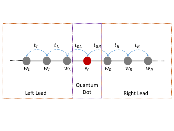
Figure 2: A single-level quantum dot coupled to two semi-infinite tight-binding leads.

where $\epsilon_{0}$ is the energy of level $|0\rangle$. A sketch of the model is shown in Fig. 2. In the wide-band limit, we find from Eq. (58) the following expressions for level-width functions and Green’s functions:

$$\Gamma_{L}^{w}= \gamma_{0L}|0\rangle\langle 0|,$$ (64)

$$\Gamma_{R}^{w}= \gamma_{0R}|0\rangle\langle 0|,$$ (65)

$$G_{CC}^{w}(E)= \frac{1}{E-\epsilon_{0}+\frac{i}{2}\gamma_{0}}|0\rangle\langle 0|,$$ (66)

$$G_{CC}^{w\dagger}(E)= \frac{1}{E-\epsilon_{0}-\frac{i}{2}\gamma_{0}}|0\rangle\langle 0|,$$ (67)

where we have introduced simplified notations $\gamma_{0\alpha}\equiv\frac{|t_{0\alpha}|^{2}}{t_{\alpha}}$ for $\alpha=L,R$ and $\gamma_{0}\equiv\gamma_{0L}+\gamma_{0R}$. The spectral function and transmission coefficient are then given by

$$A_{C}^{w}(E)= i{\rm Tr}[G_{CC}^{w}(E)-G_{CC}^{w\dagger}(E)]=\frac{\gamma_{0}}{(E-\epsilon_{0})^{2}+\frac{1}{4}\gamma_{0}^{2}}=2\pi\varrho_{C}^{w}(E),$$ (68)

$$T^{w}(E)= {\rm Tr}\left[G_{CC}^{w\dagger}(E)\Gamma_{R}^{w}(E)G_{CC}^{w}(E)\Gamma_{L}^{w}(E)\right]=\frac{\gamma_{0L}\gamma_{0R}}{(E-\epsilon_{0})^{2}+\frac{1}{4}\gamma_{0}^{2}}.$$ (69)

We see that both of them are of Lorentzian shape. In zero temperature, low bias regime, the density of states and linear conductance are determined by states at the Fermi energy:

$$\varrho_{C}^{w}(E_{F})= \frac{1}{2\pi}\frac{\gamma_{0}}{(E_{F}-\epsilon_{0})^{2}+\frac{1}{4}\gamma_{0}^{2}},$$ (70)

$${\cal C}_{0}= \frac{e^{2}}{h}\frac{\gamma_{0L}\gamma_{0R}}{(E_{F}-\epsilon_{0})^{2}+\frac{1}{4}\gamma_{0}^{2}}=\frac{e^{2}}{\hbar}\frac{\gamma_{0L}\gamma_{0R}}{\gamma_{0L}+\gamma_{0R}}\varrho_{C}^{w}(E_{F}).$$ (71)

The maximum of linear conductance is reached when the energy of an incoming electron matches the energy of the quantum dot $\epsilon_{0}$. In this case, we obtain the resonant transmission coefficient:

$$T^{w}(E)=\frac{4\gamma_{0L}\gamma_{0R}}{(\gamma_{0L}+\gamma_{0R})^{2}},$$ (72)

which is always equal to $1$ if the dot-lead coupling is symmetric ($\gamma_{0L}=\gamma_{0R}$), no matter how strong (or weak) of the coupling is.

7.2 Double-level quantum dot: spectral function and transmission coefficient

Let’s now apply the Landauer formula (42) to the electrical transport through a two-level quantum dot. The Hamiltonian of the quantum dot is given by

$$H_{CC}=\epsilon_{0}|0\rangle\langle 0|+\epsilon_{1}|1\rangle\langle 1|+t_{c}(|0\rangle\langle 1|+|1\rangle\langle 0|)=\begin{bmatrix}\epsilon_{0}&t_{c}\\ t_{c}&\epsilon_{1}\end{bmatrix}.$$ (73)

where $\epsilon_{0,1}$ are energies of decoupled levels $|0\rangle,|1\rangle$ and $t_{c}$ is the coupling strength between the two levels. In the wide-band limit, we find from Eq. (58) the following expressions for level-width function and Green’s function:

$$\Gamma_{L}^{w}=\begin{bmatrix}\frac{|t_{0L}|^{2}}{t_{L}}&0\\ 0&\frac{|t_{1L}|^{2}}{t_{L}}\end{bmatrix}\qquad\Gamma_{R}^{w}=\begin{bmatrix}\frac{|t_{0R}|^{2}}{t_{R}}&0\\ 0&\frac{|t_{1R}|^{2}}{t_{R}}\end{bmatrix},$$ (74)

$$G_{CC}^{w}(E)= \frac{1}{(E-\epsilon_{0}+i\gamma_{0})(E-\epsilon_{1}+i\gamma_{1})-t_{c}^{2}}\begin{bmatrix}E-\epsilon_{1}+i\gamma_{1}&t_{c}\\ t_{c}&E-\epsilon_{0}+i\gamma_{0}\end{bmatrix},$$ (75)

$$G_{CC}^{w\dagger}(E)= \frac{1}{(E-\epsilon_{0}-i\gamma_{0})(E-\epsilon_{1}-i\gamma_{1})-t_{c}^{2}}\begin{bmatrix}E-\epsilon_{1}-i\gamma_{1}&t_{c}\\ t_{c}&E-\epsilon_{0}-i\gamma_{0}\end{bmatrix},$$ (76)

where we have introduced the simplified notations $\gamma_{\mu}=\frac{|t_{\mu L}|^{2}}{2t_{L}}+\frac{|t_{\mu R}|^{2}}{2t_{R}}$ for $\mu=0,1$. The spectral function and transmission coefficient are then given by

$$A_{C}^{w}(E)=-2{\rm Im}{\rm Tr}[G_{CC}^{w}(E)]=-2{\rm Im}\left[\frac{(E-\epsilon_{0}+i\gamma_{0})+(E-\epsilon_{1}+i\gamma_{1})}{(E-\epsilon_{0}+i\gamma_{0})(E-\epsilon_{1}+i\gamma_{1})-t_{c}^{2}}\right],$$ (77)

$$T^{w}(E)= \frac{1}{|(E-\epsilon_{0}+i\gamma_{0})(E-\epsilon_{1}+i\gamma_{1})-t_{c}^{2}|^{2}}$$

$$\times {\rm Tr}\left(\begin{bmatrix}E-\epsilon_{1}-i\gamma_{1}&t_{c}\\ t_{c}&E-\epsilon_{0}-i\gamma_{0}\end{bmatrix}\begin{bmatrix}\frac{|t_{0R}|^{2}}{t_{R}}&0\\ 0&\frac{|t_{1R}|^{2}}{t_{R}}\end{bmatrix}\begin{bmatrix}E-\epsilon_{1}+i\gamma_{1}&t_{c}\\ t_{c}&E-\epsilon_{0}+i\gamma_{0}\end{bmatrix}\begin{bmatrix}\frac{|t_{0L}|^{2}}{t_{L}}&0\\ 0&\frac{|t_{1L}|^{2}}{t_{L}}\end{bmatrix}\right).$$ (78)

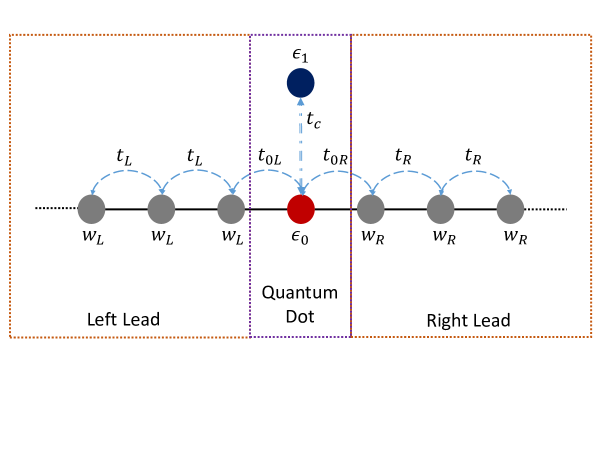
Figure 3: A double-level quantum dot coupled to semi-infinite tight-binding leads. The leads only couple to one of the two levels, forming a T-shape junction.

To simplify these expressions, we focus on a minimum extension of single-level quantum dot, i.e., only one level of the two-level quantum dot is coupled to the lead. Our LCR system then forms a “T-junction” as shown in Fig. 3. In this case, we may set $t_{1L}=t_{1R}=0$, which also results in $\gamma_{1}=0$. Furthermore, we consider a symmetric dot-lead coupling by setting $\frac{|t_{0L}|^{2}}{t_{L}}=\frac{|t_{0R}|^{2}}{t_{R}}=\gamma_{0}$. With these simplifications, we obtain the following expressions for the spectral function $A_{C}^{w}(E)$ and transmission coefficient $T^{w}(E)$ of the quantum dot:

$$A_{C}^{w}(E)= 2\gamma_{0}\frac{1+\frac{t_{c}^{2}}{(E-\epsilon_{1})^{2}}}{\left(E-\epsilon_{0}-\frac{t_{c}^{2}}{E-\epsilon_{1}}\right)^{2}+\gamma_{0}^{2}},$$ (79)

$$T^{w}(E)= \frac{\gamma_{0}^{2}}{\left(E-\epsilon_{0}-\frac{t_{c}^{2}}{E-\epsilon_{1}}\right)^{2}+\gamma_{0}^{2}}.$$ (80)

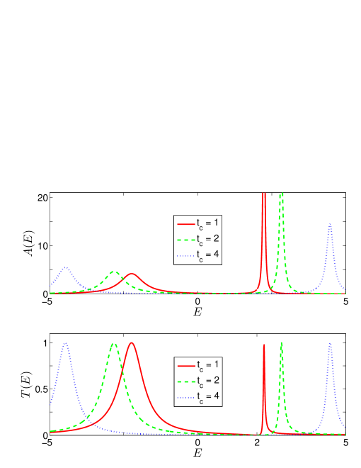
Figure 4: Spectral function $A(E)$ and transmission coefficient $T(E)$ of the double-level quantum dot coupled to semi-infinite tight-binding leads in wide-band limit. System parameters are $\epsilon_{0}=-2$, $\epsilon_{1}=2$ and $\gamma_{0}=0.5$. Only level $\epsilon_{0}$ is coupled to the leads as shown in Fig. 3. The results for three different coupling strengths between the two levels of the quantum dot are shown.

We see that none of these functions are of Lorentzian shape. Moreover, the transmission $T^{w}(E)=0$ if $E=\epsilon_{1}$. This is an anti-resonance effect. Roughly speaking, an incoming electron has two possible paths to go through the “T-junction” quantum dot. We denote them by our localized basis as (i) $|-1,0\rangle\rightarrow|0\rangle\rightarrow|1,0\rangle$ and (ii) $|-1,0\rangle\rightarrow|0\rangle\rightarrow|1\rangle\rightarrow|0\rangle\rightarrow|1,0\rangle$. Along path (i), the incident electron will reach level $\epsilon_{0}$ and then directly go through the quantum dot. Along path (ii), it will first hop from level $\epsilon_{0}$ to $\epsilon_{1}$ through the coupling $t_{c}$, and then hop back to the level $\epsilon_{0}$. If the energy $E$ of the incoming electron matches $\epsilon_{1}$, waves separately following the two paths in the quantum dot will have a $\pi$ phase difference when they meet with each other at the level $\epsilon_{0}$, resulting in a destructive interference. Therefore, under the condition $E=\epsilon_{1}$, we have a coherence-induced destruction of tunneling in this simple example. In Fig. 4, the spectral and transmission functions for three different values of the coupling strength $t_{c}$ between two levels of the quantum dot are shown. In all cases, we observe clear collapses of the transmission coefficient at $E=\epsilon_{1}$.

In low bias regime at zero temperature, the density of states and linear conductance of this model are also determined by states at the Fermi energy:

$$\varrho_{C}^{w}(E_{F})= \frac{\gamma_{0}}{\pi}\frac{1+\frac{t_{c}^{2}}{(E_{F}-\epsilon_{1})^{2}}}{\left(E_{F}-\epsilon_{0}-\frac{t_{c}^{2}}{E_{F}-\epsilon_{1}}\right)^{2}+\gamma_{0}^{2}},$$ (81)

$${\cal C}_{0}= \frac{e^{2}}{h}\frac{\gamma_{0}^{2}}{\left(E_{F}-\epsilon_{0}-\frac{t_{c}^{2}}{E_{F}-\epsilon_{1}}\right)^{2}+\gamma_{0}^{2}}=\frac{e^{2}}{\hbar}\frac{1}{2}\frac{\gamma_{0}}{1+\frac{t_{c}^{2}}{(E_{F}-\epsilon_{1})^{2}}}\varrho_{C}^{w}(E_{F}).$$ (82)

With respect to $E_{F}$, both of them have two peaks in quite different shapes, originating from nontrivial effects of quantum coherence in the system.

8 Current across a tight-binding chain: metal-insulator transitions

The formulas we summarized in the collection of Eq. (58) are also appropriate for the study of linear transport in a tight-binding chain. In this case, we make the following choices for level-width function (in wide-band limit):

$$\Gamma_{L}^{w}=\frac{|t_{CL}|^{2}}{t_{L}}|0\rangle\langle 0|,\qquad\Gamma_{R}^{w}=\frac{|t_{CR}|^{2}}{t_{R}}|N-1\rangle\langle N-1|,$$ (83)

that is, the left (right) lead is only coupled to the first (last) site of the central system. The Hamiltonian $H_{CC}$ describing the system of our interest will be chosen to have the following form:

$$H_{CC}=\sum_{\mu=0}^{N-1}\epsilon_{\mu}|\mu\rangle\langle\mu|+t_{C}\sum_{\mu=0}^{N-2}\left(|\mu\rangle\langle\mu+1|+{\rm h.c.}\right),$$ (84)

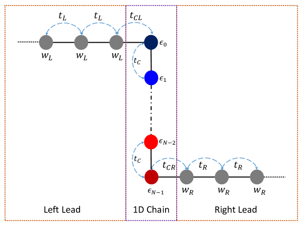
Figure 5: A tight-binding chain coupled to semi-infinite tight-binding leads at its two boundary sites.

which represents a typical tight-binding chain with onsite potential $\{\epsilon_{\mu}|\mu=0,...,N-1\}$ and nearest neighbor hopping $t_{C}$ (Other situations may include long-range, complex and site-dependent hopping amplitudes. But it should be straightforward to generalize the treatment here to those more complicated cases). The configuration of this LRC system is illustrated in Fig. 5. The retarded Green’s function, spectral function and transmission coefficient of the tight-binding chain are the computed by the following formulas:

$$G_{CC}^{w}(E)= \frac{1}{E-H_{CC}+\frac{i}{2}\left(\gamma_{L}|0\rangle\langle 0|+\gamma_{R}|N-1\rangle\langle N-1|\right)},$$ (85)

$$A_{C}^{w}(E)= i{\rm Tr}[G_{CC}^{w}(E)-G_{CC}^{w\dagger}(E)],$$ (86)

$$T^{w}(E)= \gamma_{L}\gamma_{R}|\langle N-1|G_{CC}^{w}(E)|0\rangle|^{2}.$$ (87)

where $\gamma_{\alpha}=\frac{|t_{C\alpha}|^{2}}{t_{\alpha}}$ for $\alpha=L,R$. The last equality is obtained from Eq. (43). As a useful observation, the transmission property of $H_{CC}$ at a given energy $E$ is simply determined by a single corner matrix element $\langle N-1|G_{CC}^{w}(E)|0\rangle$ of the retarded Green’s function.

To give an explicit demonstration, we consider the onsite potential of $H_{CC}$ to have the following expression:

$$\epsilon_{\mu}=\epsilon\cos\left(2\pi\frac{p}{q}\mu-k_{y}\right)\qquad\mu=0,...,N-1\qquad p,q\in\mathbb{Z}.$$ (88)

Here $k_{y}\in[0,2\pi)$ is a phase shift of the onsite potential, which will be given a concrete physical meaning in our next example. With this choice, the Hamiltonian of our central system is explicitly given by:

$$H_{{\rm AAH}}=\epsilon\sum_{\mu=0}^{N-1}\cos\left(2\pi\frac{p}{q}\mu-k_{y}\right)|\mu\rangle\langle\mu|+t_{C}\sum_{\mu=0}^{N-2}\left(|\mu\rangle\langle\mu+1|+{\rm h.c.}\right).$$ (89)

It is usually called Aubry-André-Harper (AAH) model, which has been thoroughly explored in the study of metal-insulator transitions. Its two-dimensional parent model, often called the Hofstadter model, is also a popular prototype in the study quantum Hall effects and topological insulators.

As discussed in previous sections, at zero temperature, the linear transport properties of $H_{{\rm AAH}}$ is determined by its spectral function $A_{C}^{w}(E)$ and transmission coefficient $T^{w}(E)$ evaluated at the Fermi energy $E_{F}$, giving us:

$$A_{C}^{w}(E_{F})= i{\rm Tr}[G_{CC}^{w}(E_{F})-G_{CC}^{w\dagger}(E_{F})],$$ (90)

$$T^{w}(E_{F})= \gamma_{L}\gamma_{R}|\langle N-1|G_{CC}^{w}(E_{F})|0\rangle|^{2}.$$ (91)

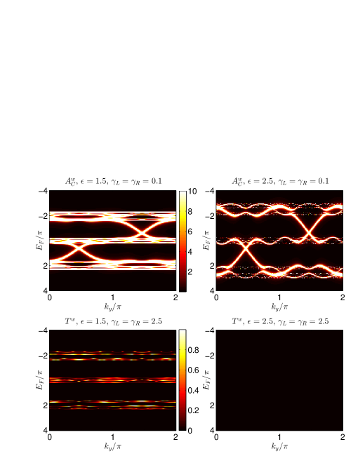
Figure 6: Spectral function $A_{C}^{w}(E_{F})$ and transmission coefficient $T^{w}(E_{F})$ of the AAH model at zero temperature in zero bias, wide-band limit. Results are shown for two different values of onsite potential $\epsilon=1.5$ and $2.5$. For spectral function, we take $\gamma_{L}=\gamma_{R}=0.1$. For transmission coefficient, we take $\gamma_{L}=\gamma_{R}=2.5$. The other system parameters are $t_{C}=1$, $\frac{p}{q}=\frac{\sqrt{5}-1}{2}$, and $N=59$.

In Fig. 6, we show the numerical results of these two functions with respect to $E_{F}$ and $k_{y}$ for two typical cases. There are third points to mention. First, in the plots for spectral function $A_{C}^{w}(E_{F})$, the states traversing the gaps are chiral edge modes. These modes are localized at the edges of the AAH chain and therefore cannot contribute to the transport, as reflected in the lower panels for the transmission coefficient $T^{w}(E_{F})$. Second, there is a metal-insulator phase transition at $\epsilon=2t_{C}$ for an irrational $\alpha$. When $\epsilon<2t_{C}$ ($\epsilon>2t_{C}$), the bulk states (bright regions) separated by gaps in $A_{C}^{w}(E_{F})$ are conducting (insulating) with non-vanishing (vanishing) transmission coefficients $T^{w}(E_{F})$. Third, resolutions of edge mode in spectral function are better for weaker couplings. Since the couplings are introduced at the boundary of the AAH chain, it is expected that a strong system-lead coupling will make the edge states less observable. On the contrary, to get better transmission properties, we need to choose couplings $\gamma_{L,R}$ closer to the energy range of the central system.

9 Current along the edge of a two-dimensional lattice: topologically quantized transport

As a final example of these notes, we will apply the Landauer formula to compute the conductance of a two-dimensional lattice. We choose the Hofstadter model (the parent of AAH model) as the central system of our interest. It describes noninteracting electrons hopping on a two-dimensional square lattice in a perpendicular magnetic field. In real space, the Hamiltonian is given by:

$$H_{CC}=t_{x}\sum_{x=0}^{N_{x}-2}\sum_{y=0}^{N_{y}-1}\left(|x\rangle\langle x+1|\otimes|y\rangle\langle y|+{\rm h.c.}\right)+t_{y}\sum_{x=0}^{N_{x}-1}\sum_{y=0}^{N_{y}-2}\left(e^{-i2\pi\frac{p}{q}x}|x\rangle\langle x|\otimes|y\rangle\langle y+1|+{\rm h.c.}\right),$$ (92)

where $t_{x}$ ($t_{y}$) is the nearest neighbor hopping amplitude along $x$ ($y$) direction of the lattice. The system contains $(N_{x}+1)\times(N_{y}+1)$ lattice sites. This model can be reduced to the AAH model if we take periodic boundary conditions along $y$-direction, and interpreting the parameter $k_{y}$ in the AAH model as the quasimomentum along $y$-direction.

To evaluate the current, we now couple the central system described by Hamiltonain (92) to leads. On the left hand side of $H_{CC}$, each lattice site $(0,y)$ for $y=0,1,...,N_{y}-1$ is coupled to a semi-infinite tight-binding chain extends from $(-\infty,y)$ to $(-1,y)$. On the right hand side of $H_{CC}$, each lattice site $(N_{x}-1,y)$ for $y=0,1,...,N_{y}-1$ is also coupled to a semi-infinite tight-binding chain extends from $(N_{x},y)$ to $(+\infty,y)$. The configuration of this LRC system is illustrated in Fig. 7. In the wide-band limit, the left and right level-width functions are given by:

$$\Gamma_{L}^{w}= |0\rangle\langle 0|\otimes\sum_{y=0}^{N_{y}-1}\gamma_{yL}|y\rangle\langle y|,$$ (93)

$$\Gamma_{R}^{w}= |N_{x}-1\rangle\langle N_{x}-1|\otimes\sum_{y=0}^{N_{y}-1}\gamma_{yR}|y\rangle\langle y|,$$ (94)

where we took $\gamma_{y\alpha}=\frac{|t_{y\alpha}|^{2}}{t_{\alpha}}$ for $\alpha=L,R$. The Hamiltonian $H_{CC}$, together with level-width functions $\Gamma_{L,R}^{w}$, determines the retarded Green’s function, spectral function and transmission coefficient of the central region:

$$G_{CC}^{w}(E)=\frac{1}{E-H_{CC}+\frac{i}{2}\sum_{y=0}^{N_{y}-1}\left(\gamma_{yL}|0\rangle\langle 0|+\gamma_{yR}|N_{x}-1\rangle\langle N_{x}-1|\right)\otimes|y\rangle\langle y|},$$ (95)

$$A_{C}^{w}(E)= -2{\rm Im}\{{\rm Tr}[G_{CC}^{w}(E)]\},$$ (96)

$$T^{w}(E)= {\rm Tr}\left[G_{CC}^{w\dagger}(E)\Gamma_{R}^{w}(E)G_{CC}^{w}(E)\Gamma_{L}^{w}(E)\right]$$

$$= \sum_{y,y^{\prime}=0}^{N_{y}-1}\gamma_{yL}\gamma_{y^{\prime}R}|\langle N_{x}-1,y^{\prime}|G_{CC}^{w}(E)|0,y\rangle|^{2}.$$ (97)

The transmission coefficient $T^{w}(E)$ has a transparent interpretation as summation over scattering amplitudes from left ($x=0$) to right ($x=N_{x}-1$) edges for all possible incoming and outgoing sites.

As a demonstration of these formulas, we consider the transmission coefficient of Hofstadter model at zero temperature in zero bias limit. For $p/q=1/3$ and $p/q=1/5$, numerical results for $T^{w}(E_{F})$ vs. $E_{F}$ are shown in Fig. 8. In both cases, we observed quantized transmission coefficients (and therefore conductances) in the spectral gap of the system. As illustrated in the plots of spectral function. current-carrying states in the gap are chiral edge modes localized at the boundary of the two-dimensional lattice. The quantization of edge state conductance in a spectral gap of the Hofstadter model is topological, equaling to the summation of bulk band Chern numbers below the considered gap. This bulk-edge correspondence principle holds in general for noninteracting fermionic Chern insulators. Interested readers can consult Ref.[9] for more details.

10 Summary and plan for future extensions

In these notes, we give a brief introduction to matrix Green’s function, focusing on its applications to steady state transport in discrete level quantum systems without many-body interactions. The Landauer formula is derived from a naive scattering viewpoint, and then applied to compute linear conductance of a single-level quantum dot, a double-level quantum dot, a tight-binding chain and a two-dimensional tight-binding lattice at zero temperature under wide-band limit. Even though a lot of approximations and simplifications have been made, the results still demonstrate the important roles of resonance, coherence, disorder and topology in quantum transport.

Further extensions of these notes may include the following topics:

• Steady state transport in periodically driven quantum systems: a combination of Green’s function and Floquet formalism

• Initial states with inter-channel coherence

• Effects of finite temperature and many-body interaction

• Quantum pumping

Acknowledgments

L. Zhou thanks Prof. Jian-Sheng Wang for his pedagogical lectures on NEGF, and helpful discussions with Prof. Jiangbin Gong and Mr. Han Hoe Yap, which motivated the preparation of these notes.

Figure 1: Real part (red solid line) and imaginary part (blue dashed line) of the lead $\alpha$’s self-energy $\Sigma_{\alpha}$, plotted with respect to the difference between the energy of incoming electron $E$ and the band center $w_{\alpha}$ of lead $\alpha$.

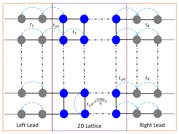
Figure 7: A two-dimensional lattice (Hofstadter model) coupled to semi-infinite tight-binding leads at its left and right boundary sites.

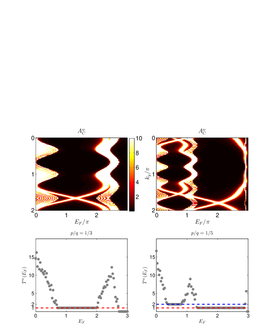
Figure 8: Transmission coefficients of the Hofstadter model at different $E_{F}$ for $p/q=1/3$ and $p/q=1/5$. The other system parameters are chosen as $N_{x}=N_{y}=44$, $t_{x}=t_{y}=1$ and $\gamma_{yL}=\gamma_{yR}=1$. The upper panels show spectral functions calculated for the two cases with periodic boundary conditions along $y$-direction. Bright lines traversing the spectral gaps represent chiral edge modes. The lower panels show numerically evaluated transmission coefficients vs. Fermi energy $E_{F}$ (in gray dots). Dashed lines are guide to the eye to point out the quantization of transmission coefficient (and conductance) in the spectral gap.

References

• [1] D. A. Ryndyk, Theory of Quantum Transport at Nanoscale (Springer, 2016).
• [2] R. A. Jishi, Feynman Diagram Techniques in Condensed Matter Physics (Cambridge University Press, 2014).
• [3] M. D. Ventra, Electrical Transport in Nanoscale Systems (Cambridge University Press, 2008).
• [4] J. C. Cuevas and E. Scheer, Molecular Electronics: An Introduction to Theory and Experiment (World Scientific, 2010).
• [5] J.-S. Wang, B. K. Agarwalla, H. Li and J. Thingna, Nonequilibrium Green’s function method for quantum thermal transport, Front. Phys. 9, 673-697 (2014).
• [6] M. Paulsson, Non Equilibrium Green’s Functions for Dummies: Introduction to the One Particle NEGF equations, arXiv:cond-mat/0210519 (2006).
• [7] S. Noschese, L. Pasquini, and L. Reichel, Tridiagonal Toeplitz Matrices: Properties and Novel Applications, Numerical Linear Algebra with Applications 20, 302-326 (2013).
• [8] H. Bruus and K. Flensberg, Many-Body Quantum Theory in Condensed Matter Physics (Oxford University Press, 2004).
• [9] Y. Hatsugai, Edge states in the integer quantum Hall effect and the Riemann surface of the Bloch function, Phys. Rev. B 48, 11851 (1993).
Refer to caption