Quantization Design and Channel Estimation for Massive MIMO Systems with One-Bit ADCs

Abstract

We consider the problem of channel estimation for uplink multiuser massive MIMO systems, where, in order to significantly reduce the hardware cost and power consumption, one-bit analog-to-digital converters (ADCs) are used at the base station (BS) to quantize the received signal. Channel estimation for one-bit massive MIMO systems is challenging due to the severe distortion caused by the coarse quantization. It was shown in previous studies that an extremely long training sequence is required to attain an acceptable performance. In this paper, we study the problem of optimal one-bit quantization design for channel estimation in one-bit massive MIMO systems. Our analysis reveals that, if the quantization thresholds are optimally devised, using one-bit ADCs can achieve an estimation error close to (with an increase by a factor of $\pi/2$) that of an ideal estimator which has access to the unquantized data. The optimal quantization thresholds, however, are dependent on the unknown channel parameters. To cope with this difficulty, we propose an adaptive quantization (AQ) approach in which the thresholds are adaptively adjusted in a way such that the thresholds converge to the optimal thresholds, and a random quantization (RQ) scheme which randomly generate a set of nonidentical thresholds based on some statistical prior knowledge of the channel. Simulation results show that, our proposed AQ and RQ schemes, owing to their wisely devised thresholds, present a significant performance improvement over the conventional fixed quantization scheme that uses a fixed (typically zero) threshold, and meanwhile achieve a substantial training overhead reduction for channel estimation. In particular, even with a moderate number of pilot symbols (about 5 times the number of users), the AQ scheme can provide an achievable rate close to that of the perfect channel state information (CSI) case.

I Introduction

Massive multiple-input multiple-output (MIMO), also known as large-scale or very-large MIMO, is a promising technology to meet the ever growing demands for higher throughput and better quality-of-service of next-generation wireless communication systems [1, 2, 3]. Massive MIMO systems are those that are equipped with a large number of antennas at the base station (BS) simultaneously serving a much smaller number of single-antenna users sharing the same time-frequency slot. By exploiting the asymptotic orthogonality among channel vectors associated with different users, massive MIMO systems can achieve almost perfect inter-user interference cancelation with a simple linear precoder and receive combiner [4], and thus have the potential to enhance the spectrum efficiency by orders of magnitude.

Despite all these benefits, massive MIMO systems pose new challenges for system design and hardware implementation. Due to the large number of antennas at the BS, the hardware cost and power consumption could become prohibitively high if we still employ expensive and power-hungry high-resolution analog-to-digital convertors (ADCs) [5]. To address this obstacle, recent studies (e.g. [6, 7, 8, 9, 10, 11, 12]) considered the use of low-resolution ADCs (e.g. 1-3 bits) for massive MIMO systems. It is known that the hardware complexity and power consumption grow exponentially with the resolution (i.e. the number of bits per sample) of the ADC. Therefore lowering the resolution of the ADC can effectively reduce the hardware cost and power consumption. In particular, for the extreme one-bit case, the ADC becomes a simple analog comparator. Also, automatic gain control (AGC) is no longer needed when one-bit ADCs are used, which further simplifies the hardware complexity.

Massive MIMO with low-resolution ADCs has attracted much attention over the past few years. Great efforts have been made to understand the effects of low-resolution ADCs on the performance of MIMO and massive MIMO systems. Specifically, by assuming full knowledge of channel state information (CSI), the capacity at both finite and infinite signal-to-noise ratio (SNR) was derived in [13] for one-bit MIMO systems. For massive MIMO systems with low-resolution ADCs, the spectral efficiency and the uplink achievable rate were investigated in [6, 7, 8, 14] under different assumptions. The theoretical analyses suggest that the use of the low cost and low-resolution ADCs can still provide satisfactory achievable rates and spectral efficiency.

In this paper, we consider the problem of channel estimation for uplink multiuser massive MIMO systems, where one-bit ADCs are used at the BS in order to reduce the cost and power consumption. Channel estimation is crucial to support multi-user MIMO operation in massive MIMO systems [15, 16, 17, 18, 19]. To reach the full potential of massive MIMO, accurate downlink CSI is required at the BS for precoding and other operations. Most literature on massive MIMO systems, e.g. [4, 1, 20, 21], assumes a time division duplex (TDD) mode in which the downlink CSI can be immediately obtained from the uplink CSI by exploiting channel reciprocity. Nevertheless, channel estimation for massive MIMO systems with one-bit ADCs is challenging since the magnitude and phase information about the received signal are lost or severely distorted due to the coarse quantization. It was shown in [6] that one-bit massive MIMO systems require an excessively long training sequence (e.g. approximately 50 times the number of users) to achieve an acceptable performance. The work [9] showed that for one-bit massive MIMO systems, a least-squares channel estimation scheme and a maximum-ratio combining scheme are sufficient to support both multiuser operation and the use of high-order constellations. Nevertheless, a long training sequence is still a requirement. To alleviate this issue, a Bayes-optimal joint channel and data estimation scheme was proposed in [11], in which the estimated payload data are utilized to aid channel estimation. In [12], a maximum likelihood channel estimator, along with a near maximum likelihood detector, were proposed for uplink massive MIMO systems with one-bit ADCs.

Despite these efforts, channel estimation using one-bit quantized data still incur much larger estimation errors as compared with using the original unquantized data, and require considerably higher training overhead to attain an acceptable estimation accuracy. To address this issue, in this paper, we study one-bit quantizer design and examine the impact of the choice of quantization thresholds on the estimation performance. Specifically, the optimal design of quantization thresholds as well as the training sequences is investigated. Note that one-bit quantization design is an interesting and important issue but largely neglected by existing massive MIMO channel estimation studies. In fact, most channel estimation schemes, e.g. [6, 9, 11, 12], assume a fixed, typically zero, quantization threshold. The optimal choice of the quantization threshold was considered in [22, 23], but addressed from an information-theoretic perspective. Our theoretical results reveal that, given that the quantization thresholds are optimally devised, using one-bit ADCs can achieve an estimation error close to (with an increase only by a factor of $\pi/2$) the minimum achievable estimation error attained by using infinite-precision ADCs. The optimal quantization thresholds, however, are dependent on the unknown channel parameters. To cope with this difficulty, we propose an adaptive quantization (AQ) scheme by which the thresholds are dynamically adjusted in a way such that the thresholds converge to the optimal thresholds, and a random quantization (RQ) scheme which randomly generates a set of non-identical thresholds based on some statistical prior knowledge of the channel. Simulation results show that our proposed schemes, because of their wisely devised quantization thresholds, present a significant performance improvement over the fixed quantization scheme that use a fixed (say, zero) quantization threshold. In particular, the AQ scheme, even with a moderate number of pilot symbols (about 5 times the number of users), can provide an achievable rate close to that of the perfect CSI case.

The rest of the paper is organized as follows. The system model and the problem of channel estimation using one-bit ADCs are discussed in Section II. In Section III, we develop a maximum likelihood estimator and carry out a Cramér-Rao bound analysis of the one-bit channel estimation problem. The optimal design of quantization thresholds and the pilot sequences is studied in Section IV. In Section V, we develop an adaptive quantization scheme and a random quantization scheme for practical threshold design. Simulation results are provided in Section VI, followed by concluding remarks in Section VII.

II System Model and Problem Formulation

Consider a single-cell uplink multiuser massive MIMO system, where the BS equipped with $M$ antennas serves $K$ ($M\gg K$) single-antenna users simultaneously. The channel is assumed to be flat block fading, i.e. the channel remains constant over a certain amount of coherence time. The received signal at the BS can be expressed as

$$\boldsymbol{Y}=\boldsymbol{H}\boldsymbol{X}+\boldsymbol{W}$$ (1)

where $\boldsymbol{X}\in\mathbb{C}^{K\times L}$ is a training matrix and its row corresponds to each user’s training sequence with $L$ pilot symbols, $\boldsymbol{H}\in\mathbb{C}^{M\times K}$ denotes the channel matrix to be estimated, and $\boldsymbol{W}\in\mathbb{C}^{M\times L}$ represents the additive white Gaussian noise with its entries following a circularly symmetric complex Gaussian distribution with zero mean and variance $2\sigma^{2}$.

To reduce the hardware cost and power consumption, we consider a massive MIMO system which uses one-bit ADCs at the BS to quantize the received signal. Specifically, at each antenna, the real and imaginary components of the received signal are quantized separately using a pair of one-bit ADCs. Thus in total $2M$ one-bit ADCs are needed. The quantized output of the received signal, $\boldsymbol{B}\triangleq[b_{m,l}]$, can be written as

$$\boldsymbol{B}=\mathcal{Q}(\boldsymbol{Y})$$ (2)

where $\mathcal{Q}(\boldsymbol{Y})$ is an element-wise operation performed on $\boldsymbol{Y}$, and for each element of $\boldsymbol{Y}$, $y_{m,l}$, we have

$$\mathcal{Q}(y_{m,l})=\text{sgn}(\Re(y_{m,l}))+j\text{sgn}(\Im(y_{m,l}))$$ (3)

in which $\Re(y)$ and $\Im(y)$ denote the real and imaginary components of $y$, respectively, and the sign function $\text{sgn}(\cdot)$ is defined as

$$\text{sgn}(y)\triangleq\left\{\begin{array}[]{ll}1&\textrm{if $y\geq 0$}\\ -1&\textrm{otherwise}\end{array}\right.$$ (6)

Therefore the quantized output belongs to the set

$$b_{m,l}\in\{1+j,-1+j,1-j,-1-j\}\quad\forall m,l$$ (7)

Note that in (2), we implicitly assume a zero threshold for one-bit quantization. Nevertheless, using identically a zero threshold for all measurements is not necessarily optimal, and it is interesting to analyze the impact of the quantization thresholds on the channel estimation performance. Such an issue (i.e. choice of quantization thresholds), albeit important, was to some extent neglected by most existing studies. To examine this problem, let $\boldsymbol{T}\triangleq[\tau_{m,l}]$ denote the thresholds used for one-bit quantization. The quantized output of the received signal, $\boldsymbol{B}$, is now given as

$$\boldsymbol{B}=\mathcal{Q}(\boldsymbol{Y}-\boldsymbol{T})$$ (8)

To facilitate our analysis, we first convert (1) into a real-valued form as follows

$$\boldsymbol{\widetilde{Y}}=\boldsymbol{\widetilde{A}}\boldsymbol{\widetilde{H}}+\boldsymbol{\widetilde{W}}$$ (9)

where

$$\boldsymbol{\widetilde{Y}}\triangleq [\Re(\boldsymbol{Y})\ \Im(\boldsymbol{Y})]^{T}$$

$$\boldsymbol{\widetilde{H}}\triangleq [\Re(\boldsymbol{H})\ \Im(\boldsymbol{H})]^{T}$$

$$\boldsymbol{\widetilde{W}}\triangleq [\Re(\boldsymbol{W})\ \Im(\boldsymbol{W})]^{T}$$

and

$$\boldsymbol{\widetilde{A}}\triangleq\left[\begin{array}[]{ccc}\Re(\boldsymbol{X})&\Im(\boldsymbol{X})\\ -\Im(\boldsymbol{X})&\Re(\boldsymbol{X})\end{array}\right]^{T}$$ (12)

Vectorizing the real-valued matrix $\boldsymbol{\widetilde{Y}}$, the received signal can be expressed as a real-valued vector form as

$$\boldsymbol{y}=\boldsymbol{A}\boldsymbol{h}+\boldsymbol{w}$$ (13)

where $\boldsymbol{y}\triangleq\text{vec}(\boldsymbol{\widetilde{Y}})$, $\boldsymbol{A}\triangleq\boldsymbol{I}_{M}\otimes\boldsymbol{\widetilde{A}}$, $\boldsymbol{h}\triangleq\text{vec}(\boldsymbol{\widetilde{H}})$, and $\boldsymbol{w}\triangleq\text{vec}(\boldsymbol{\widetilde{W}})$. It can be easily verified $\boldsymbol{y}\in\mathbb{R}^{2ML}$, $\boldsymbol{A}\in\mathbb{R}^{2ML\times 2MK}$, and $\boldsymbol{h}\in\mathbb{R}^{2MK}$. Accordingly, the one-bit quantized data can be written as

$$\boldsymbol{b}=\text{sgn}(\boldsymbol{y}-\boldsymbol{\tau})$$ (14)

where $\boldsymbol{\tau}\triangleq\text{vec}([\Re(\widetilde{\boldsymbol{T}})\ \Im(\widetilde{\boldsymbol{T}})]^{T})$ and $\boldsymbol{\tau}\in\mathbb{R}^{2ML}$. For simplicity, we define $N\triangleq 2ML$.

Our objective in this paper is to estimate the channel $\boldsymbol{h}$ based on the one-bit quantized data $\boldsymbol{b}$, examine the best achievable estimation performance and investigate the optimal thresholds $\boldsymbol{\tau}$ as well as the optimal training sequences $\boldsymbol{X}$. To this objective, in the following, we first develop a maximum likelihood (ML) estimator and carry out a Cramér-Rao bound (CRB) analysis. The optimal choice of the quantization thresholds as well as the training sequences is then studied based on the CRB matrix of the unknown channel parameter vector $\boldsymbol{h}$.

III ML Estimator and CRB Analysis

III-A ML Estimator

By combining (13) and (14), we have

$$b_{n}=\text{sgn}(y_{n}-\tau_{n})=\text{sgn}(\boldsymbol{a}_{n}^{T}\boldsymbol{h}+w_{n}-\tau_{n}),\quad\forall n$$ (15)

where, by allowing a slight abuse of notation, we let $b_{n}$, $y_{n}$, $\tau_{n}$, and $w_{n}$ denote the $n$th entry of $\boldsymbol{b}$, $\boldsymbol{y}$, $\boldsymbol{\tau}$, and $\boldsymbol{w}$, respectively; and $\boldsymbol{a}_{n}^{T}$ denotes the $n$th row of $\boldsymbol{A}$. It is easy to derive that

$$P(b_{n}=1;\boldsymbol{h}) =P(w_{n}\geq-(\boldsymbol{a}_{n}^{T}\boldsymbol{h}-\tau_{n});\boldsymbol{h})$$

$$=F_{w}(\boldsymbol{a}_{n}^{T}\boldsymbol{h}-\tau_{n})$$ (16)

and

$$P(b_{n}=-1;\boldsymbol{h}) =P(w_{n}<-(\boldsymbol{a}_{n}^{T}\boldsymbol{h}-\tau_{n});\boldsymbol{h})$$

$$=1-F_{w}(\boldsymbol{a}_{n}^{T}\boldsymbol{h}-\tau_{n})$$ (17)

where $F_{w}(\cdot)$ denotes the cumulative density function (CDF) of $w_{n}$, and $w_{n}$ is a real-valued Gaussian random variable with zero-mean and variance $\sigma^{2}$. Therefore the probability mass function (PMF) of $b_{n}$ is given by

$$p(b_{n};\boldsymbol{h})= [1-F_{w}(\boldsymbol{a}_{n}^{T}\boldsymbol{h}-\tau_{n})]^{(1-b_{n})/2}$$

$$\cdot[F_{w}(\boldsymbol{a}_{n}^{T}\boldsymbol{h}-\tau_{n})]^{(1+b_{n})/2}$$ (18)

Since $\{b_{n}\}$ are independent, the log-PMF or log-likelihood function can be written as

$$L(\boldsymbol{h}) \triangleq\log p(b_{1},\dots,b_{N};\boldsymbol{h})$$

$$=\sum_{n=1}^{N}\bigg{\{}\frac{1-b_{n}}{2}\log[1-F_{w}(\boldsymbol{a}_{n}^{T}\boldsymbol{h}-\tau_{n})]$$

$$\qquad\quad+\frac{1+b_{n}}{2}\log[F_{w}(\boldsymbol{a}_{n}^{T}\boldsymbol{h}-\tau_{n})]\bigg{\}}$$ (19)

The ML estimate of $\boldsymbol{h}$, therefore, is given as

$$\hat{\boldsymbol{h}}=\arg\max_{\boldsymbol{h}}\ L(\boldsymbol{h})$$ (20)

It can be proved that the log-likelihood function $L(\boldsymbol{h})$ is a concave function. Hence computationally efficient search algorithms can be used to find the global maximum. The proof of the concavity of $L(\boldsymbol{h})$ is given in Appendix A.

III-B CRB

We now carry out a CRB analysis of the one-bit channel estimation problem (14). The CRB results help understand the effect of different system parameters, including quantization thresholds as well as training sequences, on the estimation performance. We first summarize our derived CRB results in the following theorem.

Theorem 1

The Fisher information matrix (FIM) for the estimation problem (14) is given as

$$\boldsymbol{J}(\boldsymbol{h})=\sum_{n=1}^{N}g(\tau_{n},\boldsymbol{a}_{n})\boldsymbol{a}_{n}\boldsymbol{a}_{n}^{T}$$ (21)

where $g(\tau_{n},\boldsymbol{a}_{n})$ is defined as

$$g(\tau_{n},\boldsymbol{a}_{n})\triangleq\frac{f_{w}^{2}(\boldsymbol{a}_{n}^{T}\boldsymbol{h}-\tau_{n})}{F_{w}(\boldsymbol{a}_{n}^{T}\boldsymbol{h}-\tau_{n})(1-F_{w}(\boldsymbol{a}_{n}^{T}\boldsymbol{h}-\tau_{n}))}$$ (22)

in which $f_{w}(\cdot)$ denotes the probability density function (PDF) of $w_{n}$. Accordingly, the CRB matrix for the estimation problem (14) is given by

$$\text{CRB}(\boldsymbol{h})=\boldsymbol{J}^{-1}(\boldsymbol{h})=\left(\sum_{n=1}^{N}g(\tau_{n},\boldsymbol{a}_{n})\boldsymbol{a}_{n}\boldsymbol{a}_{n}^{T}\right)^{-1}$$ (23)

Proof:

See Appendix B. ∎

As is well known, the CRB places a lower bound on the estimation error of any unbiased estimator [24] and is asymptotically attained by the ML estimator. Specifically, the covariance matrix of any unbiased estimate satisfies: $\text{cov}(\hat{\boldsymbol{h}})-\text{CRB}(\boldsymbol{h})\succeq\boldsymbol{0}$. Also, the variance of each component is bounded by the corresponding diagonal element of $\text{CRB}(\boldsymbol{h})$, i.e., $\text{var}(\hat{h}_{i})\geq[\text{CRB}(\boldsymbol{h})]_{ii}$.

We observe from (23) that the CRB matrix of $\boldsymbol{h}$ depends on the quantization thresholds $\boldsymbol{\tau}$ as well as the matrix $\boldsymbol{A}$ which is constructed from training sequences $\boldsymbol{X}$ (cf. (12)). Naturally, we wish to optimize $\boldsymbol{\tau}$ and $\boldsymbol{A}$ (i.e. $\boldsymbol{X}$) by minimizing the trace of the CRB matrix, i.e. the overall estimation error asymptotically achieved by the ML estimator. The optimization therefore can be formulated as follows

$$\min_{\boldsymbol{X},\boldsymbol{\tau}}\quad \text{tr}\left\{\text{CRB}(\boldsymbol{h})\right\}=\mathrm{tr}\left\{\left(\sum_{n=1}^{N}g(\tau_{n},\boldsymbol{a}_{n})\boldsymbol{a}_{n}\boldsymbol{a}_{n}^{T}\right)^{-1}\right\}$$

s.t. $$\boldsymbol{A}=\boldsymbol{I}_{M}\otimes\boldsymbol{\widetilde{A}}$$

$$\boldsymbol{\widetilde{A}}\triangleq\left[\begin{array}[]{ccc}\Re(\boldsymbol{X})&\Im(\boldsymbol{X})\\ -\Im(\boldsymbol{X})&\Re(\boldsymbol{X})\end{array}\right]^{T}$$ (26)

$$\text{tr}(\boldsymbol{X}\boldsymbol{X}^{H})\leq P$$ (27)

where $\text{tr}(\boldsymbol{X}\boldsymbol{X}^{H})\leq P$ is a transmit power constraint imposed on the pilot signals. Such an optimization is examined in the following section, where it is shown that the optimization of $\boldsymbol{X}$ can be decoupled from the optimization of the threshold $\boldsymbol{\tau}$.

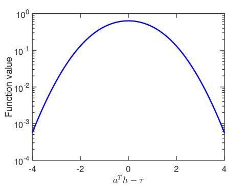
Figure 1: The function value of $g(\tau_{n},\boldsymbol{a}_{n})$ vs. $(\boldsymbol{a}_{n}^{T}\boldsymbol{h}-\tau_{n})$, where $\sigma^{2}=1$.

IV Optimal Design and Performance Analysis

IV-A Optimal Quantization Thresholds and Pilot Sequences

Before proceeding, we first introduce the following result.

Proposition 1

For the Gaussian random variable $w_{n}$, $g(\tau_{n},\boldsymbol{a}_{n})$ defined in (22) is a positive and symmetric function attaining its maximum when $\tau_{n}=\boldsymbol{a}_{n}^{T}\boldsymbol{h}$ (see Fig. 1).

Proof:

Please see Appendix C. ∎

Hence, given a fixed $\boldsymbol{A}$ (i.e. $\boldsymbol{X}$), the optimal quantization thresholds conditional on $\boldsymbol{A}$ are given by

$$\tau_{n}^{\star}=\boldsymbol{a}_{n}^{T}\boldsymbol{h},\quad\forall n\in\{1,\ldots,N\}$$ (28)

The result (28) comes directly by noting that

$$\sum_{n=1}^{N}g_{n}(\tau_{n}^{\star},\boldsymbol{a}_{n})\boldsymbol{a}_{n}\boldsymbol{a}_{n}^{T}-\sum_{n=1}^{N}g_{n}(\tau_{n},\boldsymbol{a}_{n})\boldsymbol{a}_{n}\boldsymbol{a}_{n}^{T}\succeq\mathbf{0}$$ (29)

and resorting to the convexity of $\text{tr}(\boldsymbol{P}^{-1})$ over the set of positive definite matrix, i.e. for any $\boldsymbol{P}\succ\mathbf{0}$, $\boldsymbol{Q}\succ\mathbf{0}$, and $\boldsymbol{P}-\boldsymbol{Q}\succeq\mathbf{0}$, the following inequality $\text{tr}(\boldsymbol{P}^{-1})\leq\text{tr}(\boldsymbol{Q}^{-1})$ holds (see [25]).

We see that the optimal choice of the quantization threshold $\tau_{n}$ is dependent on the unknown channel $\boldsymbol{h}$. To facilitate our analysis, we, for the time being, suppose $\boldsymbol{h}$ is known. Substituting (28) into (27) and noting that

$$g(\tau_{n}^{\star},\boldsymbol{a}_{n})=\frac{f_{w}^{2}(0)}{F_{w}(0)(1-F_{w}(0))}=\frac{2}{\pi\sigma^{2}}\quad\forall n$$ (30)

the optimization (27) reduces to

$$\min_{\boldsymbol{X}}\quad \frac{\pi\sigma^{2}}{2}\text{tr}\left\{\left(\boldsymbol{A}^{T}\boldsymbol{A}\right)^{-1}\right\}$$

s.t. $$\boldsymbol{A}=\boldsymbol{I}_{M}\otimes\boldsymbol{\widetilde{A}}$$

$$\boldsymbol{\widetilde{A}}\triangleq\left[\begin{array}[]{ccc}\Re(\boldsymbol{X})&\Im(\boldsymbol{X})\\ -\Im(\boldsymbol{X})&\Re(\boldsymbol{X})\end{array}\right]^{T}$$ (33)

$$\text{tr}(\boldsymbol{X}\boldsymbol{X}^{H})\leq P$$ (34)

which is now independent of $\boldsymbol{h}$. We have the following theorem regarding the solution to the optimization (34).

Theorem 2

The minimum achievable objective function value of (34) is given by $(\pi\sigma^{2}MK^{2})/P$ and can be attained if the pilot matrix $\boldsymbol{X}$ satisfies

$$\boldsymbol{X}\boldsymbol{X}^{H}=(P/K)\boldsymbol{I}$$ (35)

Proof:

See Appendix E. ∎

Theorem 2 reveals that, for one-bit massive MIMO systems, users should employ orthogonal pilot sequences in order to minimize channel estimation errors. Although it is a convention to use orthogonal pilots to facilitate channel estimation for conventional massive MIMO systems, to our best knowledge, its optimality in one-bit massive MIMO systems has not been established before.

IV-B Performance Analysis

We now investigate the estimation performance when the optimal thresholds are employed, and its comparison with the performance attained by a conventional massive MIMO system which assumes infinite-precision ADCs. Substituting the optimal thresholds (28) into the CRB matrix (23), we have

$$\text{CRB}_{\text{OQ}}(\boldsymbol{h})=\frac{\pi\sigma^{2}}{2}\left(\boldsymbol{A}^{T}\boldsymbol{A}\right)^{-1}$$ (36)

where for clarity, we use the subscript OQ to represent the estimation scheme using optimal quantization thresholds. On the other hand, when the unquantized observations $\boldsymbol{y}$ are available, it can be readily verified that the CRB matrix is given as

$$\text{CRB}_{\text{NQ}}(\boldsymbol{h})=\sigma^{2}\left(\boldsymbol{A}^{T}\boldsymbol{A}\right)^{-1}$$ (37)

where we use the subscript NQ to represent the scheme which has access to the unquantized observations. Comparing (36) with (37), we can see that if optimal thresholds are employed, then using one-bit ADCs for channel estimation incurs only a mild performance loss relative to using infinite-precision ADCs, with the CRB increasing by only a factor of $\pi/2$, i.e.

$$\text{CRB}_{\text{OQ}}(\boldsymbol{h})=\frac{\pi}{2}\text{CRB}_{\text{NQ}}(\boldsymbol{h})$$ (38)

We also take a glimpse of the estimation performance as the thresholds deviate from their optimal values. For simplicity, let $\tau_{n}=\tau_{n}^{\star}+\delta=\boldsymbol{a}_{n}^{T}\boldsymbol{h}+\delta,\forall n$, in which case the CRB matrix is given by

$$\text{CRB}_{\text{Q}}(\boldsymbol{h})=\frac{F_{w}(\delta)(1-F_{w}(\delta))}{f_{w}^{2}(\delta)}\left(\boldsymbol{A}^{T}\boldsymbol{A}\right)^{-1}$$ (39)

Since $(F_{w}(\delta)(1-F_{w}(\delta)))/f_{w}^{2}(\delta)$ is the reciprocal of $g(\tau_{n},\boldsymbol{a}_{n})$, from Fig. 1, we know that the function value $(F_{w}(\delta)(1-F_{w}(\delta)))/f_{w}^{2}(\delta)$ grows exponentially as $|\delta|$ increases. This indicates that a deviation of the thresholds from their optimal values results in a substantial performance loss.

In summary, the above results have important implications for the design of one-bit massive MIMO systems. It points out that a careful choice of quantization thresholds can help improve the estimation performance significantly, and help achieve an estimation accuracy close to an ideal estimator which has access to the raw observations $\boldsymbol{y}$.

The problem lies in that the optimal thresholds $\boldsymbol{\tau}$ are functions of $\boldsymbol{h}$, as described in (28). Since $\boldsymbol{h}$ is unknown and to be estimated, the optimal thresholds $\boldsymbol{\tau}$ are also unknown. To address this difficulty, we, in the following, propose an adaptive quantization (AQ) scheme by which the thresholds are dynamically adjusted from one iteration to another, and a random quantization (RQ) schme which randomly generates a set of nonidentical thresholds based on some statistical prior knowledge of the channel.

V Practical Threshold Design Strategies

V-A Adaptive Quantization

One strategy to overcome the above difficulty is to use an iterative algorithm in which the thresholds are iteratively refined based on the previous estimate of $\boldsymbol{h}$. Specifically, at iteration $i$, we use the current quantization thresholds $\boldsymbol{\tau}^{(i)}$ to generate the one-bit observation data $\boldsymbol{b}^{(i)}$. Then a new estimate $\hat{\boldsymbol{h}}^{(i)}$ is obtained from the ML estimator (20). This estimate is then plugged in (28) to obtain updated quantization thresholds, i.e. $\boldsymbol{\tau}^{(i+1)}=\boldsymbol{A}\hat{\boldsymbol{h}}^{(i)}$, for subsequent iteration. When computing the ML estimate $\hat{\boldsymbol{h}}^{(i)}$, not only the quantized data from the current iteration but also from all previous iterations can be used. The ML estimator (20) can be easily adapted to accommodate these quantized data since the data are independent across different iterations. Due to the consistency of the ML estimator for large data records, this iterative process will asymptotically lead to optimal quantization thresholds, i.e. $\boldsymbol{\tau}^{(i)}\stackrel{{\scriptstyle i\to\infty}}{{\longrightarrow}}\boldsymbol{A}\boldsymbol{h}$. In fact, our simulation results show that the adaptive quantization scheme yields quantization thresholds close to the optimal values within only a few iterations.

For clarity, we summarize the adaptive quantization (AQ) scheme as follows.

Adaptive Quantization Scheme

1.	Select an initial quantization threshold $\boldsymbol{\tau}^{(0)}$ and the maximum number of iterations $i_{\text{max}}$.
2.	At iteration $i=1,2,\ldots$: Based on $\boldsymbol{y}$ and $\boldsymbol{\tau}^{(i)}$, calculate the new binary data $\boldsymbol{b}^{(i)}=\text{sgn}(\boldsymbol{y}-\boldsymbol{\tau}^{(i)})$.
3.	Compute a new estimate of $\boldsymbol{h}$, $\hat{\boldsymbol{h}}^{(i)}$, via (20).
4.	Calculate new thresholds according to $\boldsymbol{\tau}^{(i+1)}=\boldsymbol{A}\hat{\boldsymbol{h}}^{(i)}$.
5.	Go to Step 2 if $i<i_{\text{max}}$.

Note that during the iterative process, the channel $\boldsymbol{h}$ is assumed constant over time. Thus the AQ scheme can be used to estimate channels that are unchanged or slowly time-varying across a number of consecutive frames. For example, for the scenario where the relative speeds between the mobile terminals and the base station are slow, say, 2 meters per second, the channel coherence time could be up to tens of milliseconds, more precisely, about 60 milliseconds if the carrier frequency is set to 1GHz, according to the Clarke’s model [26]. Suppose the time duration of each frame is 10 milliseconds which is a typical value for practical LTE systems. In this case, the channel remains unchanged across 6 consecutive frames. We can use the AQ scheme to update the quantization thresholds at each frame based on the channel estimate obtained from the previous frame. In this way, we can expect that the quantization thresholds will come closer and closer to the optimal values from one frame to the next, and as a result, a more and more accurate channel estimate can be obtained.

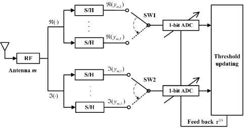
Figure 2: An off-line implementation of the AQ scheme.

The above scheme assumes a static or slowly time-varying channel across multiple frames. Another way of implementing the AQ scheme requires no such an assumption, but at the expense of increased hardware complexity. The idea is to use a number of sample-and-hold (S/H) circuits to sample the analog received signals and to store their values for subsequent offline processing. Specifically, each antenna/RF chain is followed by $2L$ S/H circuits which are equally divided into two groups to sample and store the real and imaginary components, respectively (see Fig. 2). Through a precise timing control, we ensure that at each antenna, say, the $m$th antenna, the $l$th S/H circuit pair in the two groups are controlled to store the real and imaginary components of the $l$th received pilot symbol, i.e. $\Re(y_{m,l})$ and $\Im(y_{m,l})$, respectively. Also, to avoid using a one-bit ADC for each S/H circuit, a switch can be used to connect a single one-bit ADC with multiple S/H circuits. Once the analog signals $\boldsymbol{y}$ have been stored, the AQ scheme can be implemented in an offline manner. Clearly, this offline approach can be implemented on a single frame basis, and thus no longer requires a static channel assumption. Nevertheless, such an implementation requires a number of S/H circuits as well as precise timing control for sampling and quantization. Also, this offline processing may cause a latency issue which should be taken care of in practical systems.

V-B Random Quantization

The AQ scheme requires the channel to be (approximately) stationary, or needs to be implemented with additional hardware circuits. Here we propose a random quantization (RQ) scheme that does not involve any iterative procedure and is simple to implement. The idea is to randomly generate a set of non-identical thresholds based on some statistical prior knowledge of $\boldsymbol{h}$, with the hope that some of the thresholds are close to the unknown optimal thresholds. For example, suppose each entry of $\boldsymbol{h}$ follows a Gaussian distribution with zero mean and variance $\sigma_{h}^{2}$. Note that different entries of $\boldsymbol{h}$ may have different variances due to the reason that they may correspond to different users. Nevertheless, we assume the same variance for all entries for simplicity. We randomly generate $N$ different realizations of $\boldsymbol{h}$, denoted as $\{\boldsymbol{\tilde{h}}_{n}\}$, following this known distribution. The $N$ quantization thresholds are then devised according to

$$\tau_{n}=\boldsymbol{a}_{n}^{T}\boldsymbol{\tilde{h}}_{n},\quad\forall n\in\{1,\ldots,N\}$$ (40)

Our simulation results suggest that this RQ scheme can achieve a considerable performance improvement over the conventional fixed quantization scheme which uses a fixed (typically zero) threshold. The reason is that the thresholds produced by (40) are more likely to be close to their optimal values.

VI Simulation Results

We now carry out experiments to corroborate our theoretical analysis and to illustrate the performance of our proposed one-bit quantization schemes, i.e. the AQ and the RQ schemes. We compare our schemes with the conventional fixed quantization (FQ) scheme which employs a fixed zero threshold for one-bit quantization, and a no-quantization scheme (referred to as NQ) which uses the original unquantized data for channel estimation. For the NQ scheme, it can be easily verified that its ML estimate is given by

$$\boldsymbol{\hat{h}}=(\boldsymbol{A}^{T}\boldsymbol{A})^{-1}\boldsymbol{A}^{T}\boldsymbol{y}$$ (41)

and its associated CRB is given by (37). For other schemes such as the RQ and the FQ, although a close-form expression is not available, the ML estimate can be obtained by solving the convex optimization (20). In our simulations, we assume independent and identically distributed (i.i.d.) rayleigh fading channels, i.e. all elements of $\boldsymbol{H}$ follow a circularly symmetric complex Gaussian distribution with zero mean and unit variance. Training sequences $\boldsymbol{X}$ which satisfy (35) are randomly generated. The signal-to-noise ratio (SNR) is defined as

$$\text{SNR}=\frac{P}{KL\sigma^{2}}$$ (42)

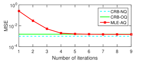
(a). $K=8$, $L=32$ and $\text{SNR}=15$ dB.

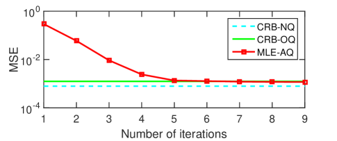
(b). $K=16$, $L=40$ and $\text{SNR}=15$ dB.

Figure 3: MSEs of the AQ scheme as a function of the number of iterations.

We first examine the estimation performance of our proposed AQ scheme which adaptively adjusts the thresholds based on the previous estimate of the channel. Fig. 3 plots the mean-squared errors (MSEs) vs. the number of iterations for the AQ scheme, where we set $K=8$, $L=32$ for Fig. (a) and $K=16$, $L=40$ for Fig. (b). The SNR is set to 15dB. The MSE is calculated as

$$\text{MSE}=\frac{1}{KM}\|\boldsymbol{H}-\boldsymbol{\hat{H}}\|_{F}^{2}$$ (43)

To better illustrate the effectiveness of the AQ scheme, we also include the CRB results in Fig. 3. in which the CRB-OQ, given by (36), represents the theoretical lower bound on the estimation errors of any unbiased estimator using optimal thresholds for one-bit quantization, and the CRB-NQ, given by (37), represents the lower bound on the estimation errors of any unbiased estimator which has access to the original observations. From Fig. 3, we see that our proposed AQ scheme approaches the theoretical lower bound CRB-OQ within only a few (say, 5) iterations, and achieves performance close to the CRB associated with the NQ scheme. This result demonstrates the effectiveness of the AQ scheme in searching for the optimal thresholds. In the rest of our simulations, we set the maximum number of iterations, $i_{\text{max}}$, equal to 5 for the AQ scheme.

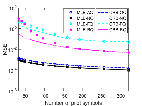
Figure 4: MSEs vs. number of pilot symbols, where $K=8$ and $\text{SNR}=15$ dB.

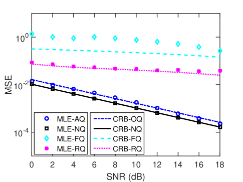
Figure 5: MSEs vs. SNR(dB), where $K=8$ and $L=96$.

We now compare the estimation performance of different schemes. Fig. 4 plots the MSEs of respective schemes as a function of the number of pilot symbols, $L$, where we set $K=8$ and $\text{SNR}=15\text{dB}$. The corresponding CRBs of these schemes are also included. Note that the CRBs for the FQ and the RQ schemes can be obtained by substituting the thresholds into (23). Results are averaged over $10^{3}$ independent runs, with the channel and the pilot sequences randomly generated for each run. From Fig. 4, we can see that the proposed AQ scheme outperforms the FQ and RQ schemes by a big margin. This result corroborates our analysis that an optimal choice of the quantization thresholds helps achieve a substantial performance improvement. In particular, the AQ scheme needs less than 30 pilot symbols to achieve a decent estimation accuracy with a MSE of 0.01, while the FQ and RQ schemes require a much larger number of pilot symbols to attain a same estimation accuracy. On the other hand, we should note that although the AQ scheme has the potential to achieve performance close to the NQ scheme, the implementation of the AQ is more complicated since it involves an iterative process to learn the optimal thresholds. In contrast, our proposed RQ scheme is as simple as the FQ scheme to implement, meanwhile it presents a clear performance advantage over the FQ scheme. We can see from Fig. 4 that the RQ requires about 100 symbols to achieve a MSE of 0.1, whereas the FQ needs about 250 pilot symbols to reach a same estimation accuracy. The reason why the RQ performs better than the FQ is that some of the thresholds produced according to (40) are likely to be close to the optimal thresholds. In Fig. 5, we plot the MSEs of respective schemes under different SNRs, where we set $K=8$ and $L=96$. Similar conclusions can be made from Fig. 5.

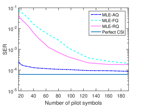
Figure 6: SERs vs. number of pilot symbols, where $K=8$, $M=64$ and $\text{SNR}=5\text{dB}$.

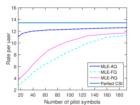
Figure 7: Achievable rates vs. number of pilot symbols, where $K=8$, $M=64$ and $\text{SNR}=5\text{dB}$.

Next, we examine the effect of channel estimation accuracy on the symbol error rate (SER) performance. For each scheme, after the channel is estimated, a near maximum likelihood detector [12] developed for one-bit massive MIMO is adopted for symbol detection. For a fair comparison, in the symbol detection stage, the quantization thresholds are all set equal to zero, as assumed in [12]. In our experiments, QPSK symbols are transmitted by all users. Fig. 6 plots the SERs of respective schemes vs. the number of pilot symbols, where we set $K=8$, $M=64$, and $\text{SNR}=5\text{dB}$. Results are averaged over all $K$ users. The SER performance obtained by assuming perfect channel knowledge is also included. It can be seen that the SER performance improves as the number of pilot symbols increases, which is expected since a more accurate channel estimate can be obtained when more pilot symbols are available for channel estimation. We also observe that the AQ scheme, using a moderate number (about 120 symbols that is only 15 times the number of users) of pilot symbols, can achieve SER performance close to that attained by assuming perfect channel knowledge. Moreover, the SER results, again, demonstrate the superiority of the RQ over the FQ scheme. In order to attain a same SER, say, $10^{-3}$, the RQ requires about 60 pilot symbols, whereas the FQ requires about 100 pilot symbols.

In Fig. 7, the achievable rates of respective schemes vs. the number of pilot symbols are depicted, where we set $K=8$, $M=64$, and $\text{SNR}=5\text{dB}$. The achievable rate for the $k$th user is calculated as [27]

$$R_{k}\triangleq\log_{2}\left(1+\frac{|\mathbb{E}\left[s_{k}^{*}(t)\hat{s}_{k}(t)\right]|^{2}}{\mathbb{E}\left[|\hat{s}_{k}(t)|^{2}\right]-|\mathbb{E}\left[s_{k}^{*}(t)\hat{s}_{k}(t)\right]|^{2}}\right)$$ (44)

where $s_{k}(t)$ is the transmit symbol of the $k$th user at time $t$, $()^{*}$ denotes the conjugate, and $\hat{s}_{k}(t)$ is the estimated symbol of $s_{k}(t)$, which is obtained via the near maximum likelihood detector by using the channel estimated by respective schemes. The achievable rate we plotted is averaged over all $K$ users. It can be seen that, even with a moderate number of pilot symbols (about 5 times the number of users), the AQ scheme can provide an achievable rate close to that of the perfect CSI case, whereas the achievable rates attained by the other two schemes are far below the level of the AQ scheme. Compared to the FQ, the RQ scheme achieves an increase of about 30 percent in the achievable rate.

VII Conclusions

Assuming one-bit ADCs at the BS, we studied the problem of one-bit quantization design and channel estimation for uplink multiuser massive MIMO systems. Specifically, based on the derived CRB matrix, we examined the impact of quantization thresholds on the channel estimation performance. Our theoretical analysis revealed that using one-bit ADCs can achieve an estimation error close to that attained by using infinite-precision ADCs, given that the quantization thresholds are optimally set. Our analysis also suggested that the optimal quantization thresholds are dependent on the unknown channel parameters. We developed two practical quantization design schemes, namely, an adaptive quantization scheme which adaptively adjusts the thresholds such that the thresholds converge to the optimal thresholds, and a random quantization scheme which randomly generates a set of non-identical thresholds based on some statistical prior knowledge of the channel. Simulation results showed that the proposed quantization schemes achieved a significant performance improvement over the fixed quantization scheme that uses a fixed (typically zero) quantization threshold, and thus can help substantially reduce the training overhead in order to attain a same estimation accuracy target.

Appendix A Proof of Concavity of The Log-Likelihood Function (19)

It can be easily verified that $f_{w}(\boldsymbol{a}_{n}^{T}\boldsymbol{h}-\tau_{n})$ is log-concave in $\boldsymbol{h}$ since the Hessian matrix of $\log f_{w}(\boldsymbol{a}_{n}^{T}\boldsymbol{h}-\tau_{n})$, which is given by

$$\frac{\partial^{2}\log f_{w}(\boldsymbol{a}_{n}^{T}\boldsymbol{h}-\tau_{n})}{{\partial\boldsymbol{h}\partial\boldsymbol{h}^{T}}}=-\frac{\boldsymbol{a}_{n}\boldsymbol{a}_{n}^{T}}{\sigma^{2}}$$ (45)

is negative semidefinite. Consequently the corresponding cumulative density function (CDF) and complementary CDF (CCDF), which are integrals of the log-concave function $f_{w}(\boldsymbol{a}_{n}^{T}\boldsymbol{h}-\tau_{n})$ over convex sets $(-\infty,\tau_{n})$ and $(\tau_{n},\infty)$ respectively, are also log-concave, and their logarithms are concave. Since summation preserves concavity, $L(\boldsymbol{h})$ is a concave function of $\boldsymbol{h}$.

Appendix B Proof of Theorem 1

Define a new variable $z_{n}\triangleq\boldsymbol{a}_{n}^{T}\boldsymbol{h}$ and define

$$l(z_{n}) \triangleq\frac{1-b_{n}}{2}\mathrm{log}[1-F_{w}(z_{n}-\tau_{n})]$$

$$\quad+\frac{1+b_{n}}{2}\mathrm{log}[F_{w}(z_{n}-\tau_{n})].$$ (46)

The first and second-order derivative of $L(\boldsymbol{h})$ are given by

$$\frac{\partial L(\boldsymbol{h})}{\partial\boldsymbol{h}}=\sum_{n=1}^{N}\frac{\partial l(z_{n})}{\partial z_{n}}\frac{\partial z_{n}}{\partial\boldsymbol{h}}=\sum_{n=1}^{N}\frac{\partial l(z_{n})}{\partial z_{n}}\boldsymbol{a}_{n}$$ (47)

and

$$\frac{\partial^{2}L(\boldsymbol{h})}{\partial\boldsymbol{h}\partial\boldsymbol{h}^{T}} =\sum_{n=1}^{N}\boldsymbol{a}_{n}\frac{\partial^{2}l(z_{n})}{\partial z_{n}^{2}}\frac{\partial z_{n}}{\partial\boldsymbol{h}^{T}}$$

$$=\sum_{n=1}^{N}\frac{\partial^{2}l(z_{n})}{\partial z_{n}^{2}}\boldsymbol{a}_{n}\boldsymbol{a}_{n}^{T}.$$ (48)

where

$$\frac{\partial l(z_{n})}{\partial z_{n}} =\frac{1-b_{n}}{2}\frac{f_{w}(z_{n}-\tau_{n})}{F_{w}(z_{n}-\tau_{n})-1}$$

$$\quad+\frac{1+b_{n}}{2}\frac{f_{w}(z_{n}-\tau_{n})}{F_{w}(z_{n}-\tau_{n})}$$ (49)

and

$$\frac{\partial^{2}l(z_{n})}{\partial z_{n}^{2}}= \frac{1-b_{n}}{2}\bigg{[}\frac{f^{\prime}_{w}(z_{n}-\tau_{n})}{F_{w}(z_{n}-\tau_{n})-1}$$

$$-\frac{f_{w}^{2}(z_{n}-\tau_{n})}{(F_{w}(z_{n}-\tau_{n})-1)^{2}}\bigg{]}+\frac{1+b_{n}}{2}$$

$$\cdot\bigg{[}\frac{f^{\prime}_{w}(z_{n}-\tau_{n})}{F_{w}(z_{n}-\tau_{n})}-\frac{f_{w}^{2}(z_{n}-\tau_{n})}{F_{w}^{2}(z_{n}-\tau_{n})}\bigg{]}$$ (50)

where $f_{w}(x)$ denotes the probability density function (PDF) of $w_{n}$, and $f^{\prime}_{w}(x)\triangleq\frac{\partial f_{w}(x)}{\partial x}$.

Therefore, the Fisher information matrix (FIM) of the estimation problem is given as

$$J(\boldsymbol{h}) =-E\left[\frac{\partial^{2}L(\boldsymbol{h})}{\partial\boldsymbol{h}\partial\boldsymbol{h}^{T}}\right]=-\sum_{n=1}^{N}E_{b_{n}}\left[\frac{\partial^{2}l(z_{n})}{\partial z_{n}^{2}}\right]\boldsymbol{a}_{n}\boldsymbol{a}_{n}^{T}$$

$$\stackrel{{\scriptstyle(a)}}{{=}}\sum_{n=1}^{N}\frac{f_{w}^{2}(\boldsymbol{a}_{n}^{T}\boldsymbol{h}-\tau_{n})}{F_{w}(\boldsymbol{a}_{n}^{T}\boldsymbol{h}-\tau_{n})(1-F_{w}(\boldsymbol{a}_{n}^{T}\boldsymbol{h}-\tau_{n}))}\boldsymbol{a}_{n}\boldsymbol{a}_{n}^{T}$$ (51)

where $E_{b_{n}}[\cdot]$ denotes the expectation with respect to the distribution of $b_{n}$, and $(a)$ follows from the fact that $b_{n}$ is a binary random variable with $P(b_{n}=1|\tau_{n},z_{n})=F_{w}(z_{n}-\tau_{n})$ and $P(b_{n}=-1|\tau_{n},z_{n})=1-F_{w}(z_{n}-\tau_{n})$. This completes the proof.

Appendix C Proof of Proposition 1

Before proceeding, we first introduce the following lemma.

Lemma 1

For $x\geq 0$, define

$$\bar{F}(x)\triangleq\int_{0}^{x}f(u)\mathrm{d}u$$ (52)

where $f(\cdot)$ denotes the PDF of a real-valued Gaussian random variable with zero-mean and unit variance. We have $\bar{F}(x)$ upper bounded by

$$\bar{F}(x)\leq\frac{1}{2}\sqrt{1-e^{-\frac{2x^{2}}{\pi}}}.$$ (53)

Proof:

See Appendix D. ∎

Define the function

$$\bar{g}(x)\triangleq\frac{f^{2}(x)}{F(x)(1-F(x))}$$ (54)

where $f(\cdot)$ and $F(\cdot)$ denotes the PDF and CDF of a real-valued Gaussian random variable with zero-mean and unit variance respectively. Invoking Lemma 1, we have

$$\bar{g}(x)=\frac{f^{2}(x)}{\frac{1}{4}-\bar{F}^{2}(x)}\leq\frac{2}{\pi}e^{-(1-\frac{2}{\pi})x^{2}}\leq\frac{2}{\pi}.$$ (55)

and $\bar{g}(x)=\frac{2}{\pi}$ if and only if $x=0$. Noting that

$$\frac{1}{\sigma^{2}}\bar{g}\left(\frac{\boldsymbol{a}_{n}^{T}\boldsymbol{h}-\tau_{n}}{\sigma}\right)=g(\tau_{n},\boldsymbol{a}_{n}).$$ (56)

Therefore $g(\tau_{n},\boldsymbol{a}_{n})$ attains its maximum when $\tau_{n}=\boldsymbol{a}_{n}^{T}\boldsymbol{h}$. The proof is completed here.

Appendix D Proof of Lemma 1

Define two i.i.d. Gaussian random variables with zero-mean and unit variance, namely, $X$ and $Y$. The joint distribution function of $X$ and $Y$ is $f_{XY}(x,y)=f(x)f(y)$. Define two regions $D_{1}\triangleq\{(u,v)\mid 0\leq u\leq x,0\leq v\leq x\}$ and $D_{2}\triangleq\{(u,v)\mid u\geq 0,v\geq 0,u^{2}+v^{2}\leq\frac{4x^{2}}{\pi}\}$. Obviously, the areas of $D_{1}$ and $D_{2}$ are the same, i.e., $\mu(D_{1})=\mu(D_{2})$, where $\mu(\cdot)$ denote the area of a region. The probabilities of $(X,Y)$ belonging in these two regions can be computed as

$$P((X,Y)\in D_{1}) =\iint_{D_{1}}f_{XY}(u,v)\mathrm{d}u\mathrm{d}v$$

$$=\bar{F}^{2}(x)$$ (57)

$$P((X,Y)\in D_{2}) =\iint_{D_{2}}f_{XY}(u,v)\mathrm{d}u\mathrm{d}v$$

$$=\frac{1}{4}\left(1-e^{-\frac{2x^{2}}{\pi}}\right)$$ (58)

Let $S_{1}\setminus S_{2}$ denote the set obtained by excluding $S_{2}\cap S_{1}$ from $S_{1}$. Clearly, we have

$$\mu(D_{1}\setminus D_{2})=\mu(D_{2}\setminus D_{1})$$ (59)

Also, according to the definition of $D_{1}$ and $D_{2}$, we have

$$f_{XY}(u,v) \leq\frac{1}{2\pi}e^{-\frac{2x^{2}}{\pi}},\quad(u,v)\in D_{1}\setminus D_{2}$$ (60)

$$f_{XY}(u,v) \geq\frac{1}{2\pi}e^{-\frac{2x^{2}}{\pi}},\quad(u,v)\in D_{2}\setminus D_{1}$$ (61)

Combining (59)–(61), we arrive at

$$\iint_{D_{1}\setminus D_{2}}f_{XY}(u,v)\mathrm{d}u\mathrm{d}v\leq\iint_{D_{2}\setminus D_{1}}f_{XY}(u,v)\mathrm{d}u\mathrm{d}v$$ (62)

From the above inequality, we have $P((X,Y)\in D_{1})\leq P((X,Y)\in D_{2})$, i.e.

$$\bar{F}^{2}(x)\leq\frac{1}{4}\left(1-e^{-\frac{2x^{2}}{\pi}}\right)\Rightarrow\bar{F}(x)\leq\frac{1}{2}\sqrt{1-e^{-\frac{2x^{2}}{\pi}}}$$ (63)

This completes the proof.

Appendix E Proof of Theorem 2

Note that from the constraint $\text{tr}(\boldsymbol{X}\boldsymbol{X}^{H})\leq P$, we can easily derive that

$$\text{tr}(\boldsymbol{A}^{T}\boldsymbol{A})\leq 2MP$$ (64)

To prove Theorem 2, let us first consider a new optimization that has the same objective function as (34) while with a relaxed constraint:

$$\min_{\boldsymbol{A}}\quad \frac{\pi\sigma^{2}}{2}\text{tr}\left\{\left(\boldsymbol{A}^{T}\boldsymbol{A}\right)^{-1}\right\}$$

s.t. $$\text{tr}(\boldsymbol{A}^{T}\boldsymbol{A})\leq 2MP$$ (65)

Clearly, the feasible region defined by the constraints in (34) is a subset of that defined by (65). Since $\text{tr}(\boldsymbol{Z}^{-1})$ is convex over the set of positive definite matrix, the optimization (65) is convex. Its optimum solution is given as follows.

Lemma 2

Consider the following optimization problem

$$\min_{\boldsymbol{Z}}\quad \text{tr}(\boldsymbol{Z}^{-1})$$

s.t. $$\text{tr}(\boldsymbol{Z})\leq P_{0}$$ (66)

where $\boldsymbol{Z}\in\mathbb{R}^{p\times p}$ is positive definite. The optimum solution to (66) is given by $\boldsymbol{Z}=(P_{0}/p)\boldsymbol{I}$ and the minimum objective function value is $p^{2}/P_{0}$.

Proof:

See Appendix F. ∎

From Lemma 2, we know that any $\boldsymbol{A}$ satisfying

$$\boldsymbol{A}^{T}\boldsymbol{A}=(P/K)\boldsymbol{I}$$ (67)

is an optimal solution to (65). Note that the set of feasible solutions (65) subsumes the feasible solution set of (34). Hence, if the optimal solution to (65) is meanwhile a feasible solution of (34), then this solution is also an optimal solution to (34). It is easy to verify that if (35) holds valid, the resulting $\boldsymbol{A}$ satisfies (67) and is thus an optimal solution to (65). As a consequence, it is also an optimal solution to (34). This completes the proof.

Appendix F Proof of Lemma 2

Let $\boldsymbol{Z}=\boldsymbol{U}\boldsymbol{D}\boldsymbol{U}^{T}$ denote the eigenvalue decomposition of $\boldsymbol{Z}$, where $\boldsymbol{U}\in\mathbb{R}^{p\times p}$ and $\boldsymbol{D}\in\mathbb{R}^{p\times p}$. By replacing $\boldsymbol{Z}$ with $\boldsymbol{U}\boldsymbol{D}\boldsymbol{U}^{T}$, the optimization (66) is reduced to determining the diagonal matrix $\boldsymbol{D}\triangleq\text{diag}(d_{1},\dots,d_{p})$

$$\min_{\{d_{i}\}}\ \sum_{i=1}^{p}\frac{1}{d_{i}}$$

s.t. $$\sum_{i=1}^{p}{d_{i}}\leq P_{0}$$

$$d_{i}>0,\qquad\forall i\in\{1,\dots,p\}$$ (68)

The Lagrangian function associated with (68) is given by

$$L(d_{i};\lambda;\nu_{i})=\sum_{i=1}^{p}\frac{1}{d_{i}}+\lambda\left(\sum_{i=1}^{p}{d_{i}}-P_{0}\right)-\sum_{i=1}^{p}{\nu_{i}d_{i}}$$ (69)

with KKT conditions [25] given as

$$-\frac{1}{d_{i}^{2}}+\lambda-\nu_{i}=0 ,\quad\forall i$$

$$\lambda\left(\sum_{i=1}^{p}{d_{i}}-P_{0}\right)=0$$

$$\lambda\geq 0$$

$$\nu_{i}d_{i}=0 ,\quad\forall i$$

$$d_{i}>0 ,\quad\forall i$$

$$\nu_{i}\geq 0 ,\quad\forall i$$

From the last three equations, we have $\nu_{i}=0$, $\forall i$. Then from the first equation we have

$$\lambda=\frac{1}{d_{i}^{2}}>0$$ (70)

and

$$d_{1}=d_{2}=\dots=d_{p}.$$ (71)

From (70) and the second equation, we have $\sum_{i=1}^{p}{d_{i}}-P_{0}=0$, from which $d_{i}$ can be readily solved as $d_{i}=P_{0}/p$, $\forall i$, i.e., the optimal $\boldsymbol{D}$ is given by $\boldsymbol{D}^{\star}=(P_{0}/p)\boldsymbol{I}$. Consequently we have $\boldsymbol{Z}^{\star}=(P_{0}/p)\boldsymbol{I}$. This completed the proof.

References

- [1] F. Rusek, D. Persson, B. K. Lau, E. G. Larsson, T. L. Marzetta, O. Edfors, and F. Tufvesson, “Scaling up MIMO: Opportunities and challenges with very large arrays,” IEEE Signal Process. Mag., vol. 30, no. 1, pp. 40–60, Jan. 2013.
- [2] E. G. Larsson, O. Edfors, F. Tufvesson, and T. L. Marzetta, “Massive MIMO for next generation wireless systems,” IEEE Commun. Mag., vol. 52, no. 2, pp. 186–195, Feb. 2014.
- [3] S. Chen, S. Sun, Q. Gao, and X. Su, “Adaptive beamforming in TDD-based mobile communication systems: State of the art and 5G research directions,” IEEE Wireless Commun., vol. 23, no. 6, pp. 81–87, Dec. 2016.
- [4] T. L. Marzetta, “Noncooperative cellular wireless with unlimited numbers of base station antennas,” IEEE Trans. Wireless Commun., vol. 9, no. 11, pp. 3590–3600, Nov. 2010.
- [5] S. Chen and J. Zhao, “The requirements, challenges, and technologies for 5G of terrestrial mobile telecommunication,” IEEE Commun. Mag., vol. 52, no. 5, pp. 36–43, May 2014.
- [6] C. Risi, D. Persson, and E. G. Larsson, “Massive MIMO with 1-bit ADC,” arXiv preprint arXiv:1404.7736, 2014.
- [7] L. Fan, S. Jin, C.-K. Wen, and H. Zhang, “Uplink achievable rate for massive MIMO systems with low-resolution ADC,” IEEE Commun. Lett., vol. 19, no. 12, pp. 2186–2189, Dec. 2015.
- [8] J. Zhang, L. Dai, S. Sun, and Z. Wang, “On the spectral efficiency of massive MIMO systems with low-resolution ADCs,” IEEE Commun. Lett., vol. 20, no. 5, pp. 842–845, May 2016.
- [9] S. Jacobsson, G. Durisi, M. Coldrey, U. Gustavsson, and C. Studer, “One-bit massive MIMO: Channel estimation and high-order modulations,” in IEEE International Conference on Communication Workshop (ICCW), London, UK, 2015, pp. 1304–1309.
- [10] S. Wang, Y. Li, and J. Wang, “Multiuser detection in massive spatial modulation MIMO with low-resolution ADCs,” IEEE Trans. Wireless Commun., vol. 14, no. 4, pp. 2156–2168, Apr. 2015.
- [11] C.-K. Wen, C.-J. Wang, S. Jin, K.-K. Wong, and P. Ting, “Bayes-optimal joint channel-and-data estimation for massive MIMO with low-precision ADCs,” IEEE Trans. Signal Processing, vol. 64, no. 10, pp. 2541–2556, May 2016.
- [12] J. Choi, J. Mo, and R. W. Heath, “Near maximum-likelihood detector and channel estimator for uplink multiuser massive MIMO systems with one-bit ADCs,” IEEE Trans. Commun., vol. 64, no. 5, pp. 2005–2018, May 2016.
- [13] J. Mo and R. W. Heath, “Capacity analysis of one-bit quantized MIMO systems with transmitter channel state information,” IEEE Trans. Signal Processing, vol. 63, no. 20, pp. 5498–5512, Oct. 2015.
- [14] N. Liang and W. Zhang, “Mixed-ADC massive MIMO,” IEEE J. Sel. Areas Commun., vol. 34, no. 4, pp. 983–997, Apr. 2016.
- [15] A. Adhikary, J. Nam, J.-Y. Ahn, and G. Caire, “Joint spatial division and multiplexing – the large-scale array regime,” IEEE Trans. Information Theory, no. 10, pp. 6441–6463, Oct. 2013.
- [16] J. Choi, D. J. Love, and P. Bidigare, “Downlink training techniques for FDD massive MIMO systems: open-loop and closed-loop training with memory,” IEEE Journal of Selected Topics in Signal Processing, no. 5, pp. 802–814, Oct. 2014.
- [17] C. Sun, X. Gao, S. Jin, M. Matthaiou, Z. Ding, and C. Xiao, “Beam division multiple access transmission for massive MIMO communications,” IEEE Trans. Communications, vol. 63, no. 6, pp. 2170–2184, June 2015.
- [18] Z. Gao, L. Dai, Z. Wang, and S. Chen, “Spatially common sparsity based adaptive channel estimation and feedback for FDD massive MIMO,” IEEE Trans. Signal Processing, no. 23, pp. 6169–6183, Dec. 2015.
- [19] J. Fang, X. Li, H. Li, and F. Gao, “Low-rank covariance-assisted downlink training and channel estimation for FDD massive MIMO systems,” IEEE Trans. Wireless Commun., vol. 16, no. 3, pp. 1935–1947, Mar. 2017.
- [20] H. Yin, D. Gesbert, M. Filippou, and Y. Liu, “A coordinated approach to channel estimation in large-scale multiple-antenna systems,” IEEE Journal on Selected Areas in Communications, no. 2, pp. 264–273, Feb. 2013.
- [21] R. R. Muller, L. Cottatellucci, and M. Vehkapera, “Blind pilot decontamination,” IEEE Journal of Selected Topics in Signal Processing, no. 5, pp. 773–786, Oct. 2014.
- [22] T. Koch and A. Lapidoth, “At low SNR, asymmetric quantizers are better,” IEEE Trans. Information Theory, vol. 59, no. 9, pp. 5421–5445, Sept. 2013.
- [23] S. Verdú, “Spectral efficiency in the wideband regime,” IEEE Trans. Information Theory, vol. 48, no. 6, pp. 1319–1343, June 2002.
- [24] S. M. Kay, Fundamentals of Statistical Signal Processing, Volume I: Estimation Theory. Upper Saddle River, NJ: Prentice Hall, 1993.
- [25] S. Boyd and L. Vandenberghe, Convex Optimization. Cambridge, UK: Cambridge University Press, 2004.
- [26] D. Tse and P. Viswanath, Fundamentals of Wireless Communication. Cambridge, UK: Cambridge University Press, 2005.
- [27] C. Mollén, J. Choi, E. G. Larsson, and R. W. Heath, “Uplink performance of wideband massive MIMO with one-bit ADCs,” IEEE Trans. Wireless Commun., vol. 16, no. 1, pp. 87–100, Jan. 2017.