Structure and Randomness of
Continuous-time, Discrete-event Processes

Abstract

Loosely speaking, the Shannon entropy rate is used to gauge a stochastic process’ intrinsic randomness; the statistical complexity gives the cost of predicting the process. We calculate, for the first time, the entropy rate and statistical complexity of stochastic processes generated by finite unifilar hidden semi-Markov models—memoryful, state-dependent versions of renewal processes. Calculating these quantities requires introducing novel mathematical objects ($\epsilon$-machines of hidden semi-Markov processes) and new information-theoretic methods to stochastic processes.

I Introduction

Claude Shannon’s seminal $1948$ article “A Mathematical Theory of Communication” introduced a definition for entropy as a well-motivated measure of randomness [1]. He further identified entropy rate $h_{\mu}$ as a measure of the minimal coding cost of a series of potentially correlated symbols in his celebrated first theorem. In $1989$, Young and Crutchfield identified statistical complexity $C_{\mu}$ as the entropy of causal states [2], which are the minimal sufficient statistics for prediction [3]. Said simply, $h_{\mu}$ is a measure of a process’ intrinsic randomness and $C_{\mu}$ a measure of process structure. In one view, these two measures of complexity are unified by the Kolmogorov-Chaitin complexity of a discrete object which is the size of the minimal Universal Turing Machine program that produces the object [4, 5]. Specifically, the expected Kolmogorov-Chaitin complexity $\langle K(x_{\ell})\rangle$ of a (discrete-time, discrete-symbol) time series $x_{\ell}$ of length $\ell$ grows at the Shannon entropy rate and has an offset determined by the statistical complexity: $\log\langle K(x_{\ell})\rangle\propto_{\ell\to\infty}C_{\mu}+\ell h_{\mu}$, when these quantities exist [6]. Both entropy rate and statistical complexity have given insight into many disparate complex systems, from chaotic crystallography [7], biomolecule dynamics [8, 9, 10], neuronal spike trains [11], and animal behavior [12] to stochastic resonance [13], geomagnetic volatility [14], hydrodynamic flows [15, 16], and fluid and atmospheric turbulence [17, 18].

Perhaps somewhat surprisingly, estimators of the entropy rate and statistical complexity of continuous-time, discrete-symbol processes are lacking. This is unfortunate since these processes are encountered very often in the physical, chemical, biological, and social sciences as sequences of discrete events consisting of an event type and an event duration or magnitude. An example critical to infrastructure design occurs in the geophysics of crustal plate tectonics, where the event types are major earthquakes tagged with time between their occurrence and with an approximate or continuous Richter magnitude [19]. Understanding these process’ randomness and structure bears directly on averting human suffering. Another example is revealed in the history of reversals of the earth’s geomagnetic field [20], which shields the planet’s life from exposure to damaging radiation. An example from physical chemistry is found in single-molecule spectroscopy which reveals molecular dynamics as hops between conformational states that persist for randomly distributed durations [10, 9]. The structure of these conformational transitions is implicated in biomolecular functioning and so key to life processes. A common example from neuroscience is found in the spike trains generated by neurons that consist of spike-no-spike event types separated by continuous interspike intervals. The structure and randomness of spike trains are key to delineating how tissues support essential information processing in nervous systems and brains [11]. Finally, a growing set of these processes appear in the newly revitalized quantitative social sciences, in which human communication events and their durations are monitored as signals of emergent coordination or competition [21].

Here, we provide entropy rate and statistical complexity estimators for continuous-time, discrete-symbol processes by first identifying the causal states of stochastic processes generated by continuous-time unifilar hidden semi-Markov models. In these processes successive dwell times for the symbols (or events) are drawn based on the process’ current “hidden” state. Transitions from hidden state to hidden state then follow a rule that mimics transitions in discrete-time unifilar hidden Markov models. The resulting output process consists of the symbols emitted during the dwell time. Identifying the process causal states leads to new expressions for entropy rate, generalizing the results of Ref. [22], and for statistical complexity. The hidden semi-Markov process class is sufficiently general that, in principle, our results yield universal estimators of the entropy rate and statistical complexity of continuous-time, discrete-event processes.

To start, we define hidden semi-Markov processes and their unifilar generators, determine their causal states, and use the causal states to calculate their entropy rate and statistical complexity. We conclude by describing a method for using the expressions given here to efficiently estimate the entropy rate and statistical complexity of real-world time series.

II Hidden Semi-Markov Processes and Their Unifilar Generators

The continuous-time, discrete-symbol process $\ldots,(X_{-1},\mathcal{T}_{-1}),(X_{0},\mathcal{T}_{0}),(X_{1},\mathcal{T}_{1}),\ldots$ has realizations $\ldots(x_{-1},\allowbreak\tau_{-1}),\allowbreak(x_{0},\tau_{0}),(x_{1},\tau_{1})\ldots$. Events are symbol-duration pairs $(x_{i},\tau_{i})$ that occur sequentially in a process. We demand that $x_{i}\neq x_{i+1}$ to enforce a unique description of the process. In other words, the discrete event symbol $x_{i}\in\mathcal{A}$ appears for a total time of $\tau_{i}$. The present is located almost surely during the emission of $x_{0}$, and we denote the time since last emission as $\tau_{0^{+}}$ and the time to next emission as $\tau_{0^{-}}$. We also, for clarity, denote the last-appearing symbol as $x_{0^{+}}$ and the next-appearing symbol as $x_{0^{-}}$; though obviously $x_{0^{+}}=x_{0^{-}}$ almost surely. (It follows that $\tau_{0^{+}}+\tau_{0^{-}}=\tau_{0}$.) The past $\ldots,(X_{-1},\mathcal{T}_{-1}),(X_{0},\mathcal{T}_{0^{+}})$ is denoted $\smash{\overleftarrow{(X,\mathcal{T})}}$ and the future $(X_{0},\mathcal{T}_{0^{-}}),(X_{1},\mathcal{T}_{1}),\ldots$ is denoted as $\smash{\overrightarrow{(X,\mathcal{T})}}$, with realizations denoted $\smash{\overleftarrow{(x,\tau)}}$ and $\smash{\overrightarrow{(x,\tau)}}$, respectively.

A continuous-time, discrete-symbol process’ causal states $\mathcal{S}$ are the equivalence classes of pasts defined by the relation:

$$\smash{\overleftarrow{(x,\tau)}}\sim_{\epsilon}{\smash{\overleftarrow{(x,\tau)}}}^{\prime}\iff\Pr\bigg{(}\smash{\overrightarrow{(X,\mathcal{T})}}\bigg{|}\smash{\overleftarrow{(X,\mathcal{T})}}=\smash{\overleftarrow{(x,\tau)}}\bigg{)}=\Pr\bigg{(}\smash{\overrightarrow{(X,\mathcal{T})}}\bigg{|}\smash{\overleftarrow{(X,\mathcal{T})}}={\smash{\overleftarrow{(x,\tau)}}}^{\prime}\bigg{)}~{}.$$ (1)

This mimics the relation for the causal states of discrete-time processes [3]. A process’ statistical complexity is the entropy of these causal states: $C_{\mu}=\operatorname{H}[\mathcal{S}]$. A process’ prescient states are any finer-grained partition of the causal-state classes, as for discrete-time processes [3]. Thus, there is a fundamental distinction between a process’ observed or emitted symbols and its internal states. In this way, we consider general processes as hidden processes.

A hidden semi-Markov process (HSMP) is a continuous-time, discrete-symbol process generated by a hidden semi-Markov model (HSMM). A HSMM is described via a hidden-state random variable $\mathcal{G}$ with realization $g$, an emission probability $T^{(x)}_{g}$ for symbol $x$, and a dwell-time distribution $\phi_{g}(\tau)$. In other words, in hidden state $g$, symbol $x$ is emitted for time $\tau$ drawn from $\phi_{g}(\tau)$. For reasons that will become clear, we focus on a restricted form—the unifilar HSMM (uHSMM). For these, the present hidden state $g_{0}$ is uniquely determined by the past emitted symbols $x_{-\infty:0}=\ldots,x_{-2},x_{-1}$. See Fig. 1. In an abuse of notation, Eq. (1) determines a function $\epsilon(x_{-\infty:0})$ that takes the past emitted symbol sequence $x_{-\infty:0}$ to the underlying hidden state $g_{0}$. (The abuse comes from suppressing the dependence on durations.) This is the analog appropriate to this setting of the familiar definition of unifilarity in discrete-time models—that symbol and state uniquely determine next state.

We assume that the underlying uHSMM has minimal size. That is, out of all such models that generate a given process, we work only with the one having the minimal number of hidden states. Due to the unifilarity constraint, minimality in the number of hidden states is equivalent to minimality in the entropy $C_{\mu}$ over the hidden states. A hidden semi-Markov process’ minimal uHSMM is its $\epsilon$-machine.

III Causal architecture

The challenge now is to identify a given HSMP’s causal states. With the causal states in hand, we can calculate their statistical complexity and entropy rate rather straightforwardly. Theorem 1 makes the identification.

Theorem 1.

A unifilar hidden semi-Markov process’ causal states are the triple $(g_{0},x_{0^{+}},\tau_{0^{+}})$, under weak assumptions.

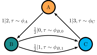
Figure 1: Generative model for a unifilar hidden semi-Markov process. The notation $p(x)|x,\tau\sim\phi_{g}$ means that $x$ is emitted with probability $p(x)$ from hidden state $g$ with emission time drawn from $\phi_{g}$.

Proof.

To identify causal states, we need to simplify the conditional probability distribution:

$$p\bigg{(}\smash{\overrightarrow{(x,\tau)}}\bigg{|}\smash{\overleftarrow{(x,\tau)}}\bigg{)}=\Pr\bigg{(}\smash{\overrightarrow{(X,\mathcal{T})}}=\smash{\overrightarrow{(x,\tau)}}\bigg{|}\smash{\overleftarrow{(X,\mathcal{T})}}=\smash{\overleftarrow{(x,\tau)}}\bigg{)}~{}.$$

When the process is generated by a unifilar hidden semi-Markov model, this conditional probability distribution simplifies to:

$$p\bigg{(}\smash{\overrightarrow{(x,\tau)}}\bigg{|}\smash{\overleftarrow{(x,\tau)}}\bigg{)} =p\big{(}(x_{0^{-}},\tau_{0^{-}}),(x_{1},\tau_{1}),\ldots\big{|}\ldots,(x_{-1},\tau_{-1}),(x_{0^{+}},\tau_{0^{+}})\big{)}$$

$$=p\big{(}(x_{1},\tau_{1}),\ldots\big{|}\ldots,(x_{0},\tau_{0})\big{)}p\big{(}\tau_{0^{-}}\big{|}\ldots,(x_{-1},\tau_{-1}),(x_{0^{+}},\tau_{0^{+}}),x_{0^{-}}\big{)}$$

$$\qquad p\big{(}x_{0^{+}}\big{|}\ldots,(x_{-1},\tau_{-1}),(x_{0^{+}},\tau_{0^{+}}),x_{0^{-}})\big{)}$$ (2)

where we have $\tau_{0}=\tau_{0^{+}}+\tau_{0^{-}}$. Almost surely, we have:

$$p\big{(}x_{0^{+}}\big{|}\ldots,(x_{-1},\tau_{-1}),(x_{0^{+}},\tau_{0^{+}}),x_{0^{-}})\big{)}=\delta_{x_{0^{+}},x_{0^{-}}}$$ (3)

and, due to the unifilarity constraint:

$$p\big{(}\tau_{0^{-}}\big{|}\ldots,(x_{-1},\tau_{-1}),(x_{0^{+}},\tau_{0^{+}}),x_{0^{-}}\big{)} =p\big{(}\tau_{0^{-}}\big{|}\tau_{0^{+}},g_{0}=\epsilon^{+}(x_{:0})\big{)}~{}.$$ (4)

Together Eqs. (2)-(4) imply that the triple $(g_{0},x_{0^{+}},\tau_{0^{+}})$ are prescient statistics.

These states are causal (minimal and prescient) when two things happen: first, when the number of hidden states $g$ is minimal; and second, when $\phi_{g}(\tau)$ does not take either the “eventually Poisson” or “eventually $\Delta$-Poisson” form described in Ref. [23]. This last condition is worth spelling out. To avoid an eventually Poisson-like dwell time distribution, we demand that $\phi_{g}(\tau)$ cannot be written as $\phi_{g}(T)e^{-\lambda(t-T)}$ for all $t\geq T$ for some $\lambda>0$ and $T\geq 0$. To avoid an eventually $\Delta$-Poisson-like dwell time distribution, we demand that $\phi_{g}(\tau)$ cannot be written as:

$$\phi_{g}(t)=\phi_{g}\big{(}T+(t-T)\!\!\!\!\mod\Delta\big{)}e^{-\lambda\lfloor(t-T)/\Delta\rfloor}~{},$$

for any $0<\Delta,\lambda,T<\infty$. Almost all naturally occurring dwell-time distributions take neither of these forms. And so, we say that the typical unifilar hidden semi-Markov process’ causal states are given by the triple $(g_{0},x_{0^{+}},\tau_{0^{+}})$.

To find a process’ statistical complexity $C_{\mu}$, we must determine $H[\mathcal{S}]$ which, in turn, entails finding the probability distribution $p(g_{0},x_{0^{+}},\tau_{0^{+}})$. Implicitly, we are deriving labeled transition operators as in Ref. [23]. We start by decomposing:

$$p(g_{0},x_{0^{+}},\tau_{0^{+}})=p(g_{0})p(x_{0^{+}}|g_{0})p(\tau_{0^{+}}|g_{0},x_{0^{+}})~{}.$$

Since the dwell-time distribution depends only on the hidden state $g_{0}$ and not on the emitted symbol $x_{0^{+}}$, we find that:

$$p(\tau_{0^{+}}|g_{0},x_{0^{+}})=p(\tau_{0^{+}}|g_{0})~{}.$$

As in Ref. [23], having a dwell time of at least $\tau_{0^{+}}$ implies that:

$$p(\tau_{0^{+}}|g_{0}) =\int_{\tau_{0^{+}}}^{\infty}p(\tau_{0}|g_{0})d\tau_{0}$$

$$=\mu_{g_{0}}\Phi_{g_{0}}(\tau_{0^{+}})~{},$$ (5)

where $\Phi_{g_{0}}(\tau_{0^{+}})$ will be called the survival distribution and is defined by Eq. (5). From the setup, we also have:

$$p(x_{0^{+}}|g_{0})=T_{g_{0}}^{(x_{0^{+}})}~{}.$$

Finally, to calculate $p(g_{0})$, we consider all ways in which probability can flow from $(g^{\prime},x^{\prime},\tau^{\prime})$ to $(g,x,0)$:

$$p(g,x,0) =\sum_{g^{\prime},x^{\prime}}\int_{0}^{\infty}p(g^{\prime},x^{\prime},\tau^{\prime})p((g^{\prime},x^{\prime},\tau^{\prime})\rightarrow(g,x,0))d\tau^{\prime}~{}.$$ (6)

The transition probability $p((g^{\prime},x^{\prime},\tau^{\prime})\rightarrow(g,x,0))$ is:

$$p((g^{\prime},x^{\prime},\tau^{\prime})\rightarrow(g,x,0))=\delta_{g,\epsilon(g^{\prime},x^{\prime})}T_{g}^{(x)}\frac{\phi_{g^{\prime}}(\tau^{\prime})}{\Phi_{g^{\prime}}(\tau^{\prime})}~{}.$$ (7)

The term $\delta_{g,\epsilon(g^{\prime},x^{\prime})}$ implies that one can only transition to $g$ from $g^{\prime}$ if the emitted symbol $x^{\prime}$ allows. Then, $T_{g}^{(x)}$ implies that there is a probability of emitting symbol $x$ from newly-transitioned-to hidden state $g$. And, $\phi_{g^{\prime}}(\tau^{\prime})/\Phi_{g^{\prime}}(\tau^{\prime})$ is the probability of emitting $x^{\prime}$ for total time $\tau^{\prime}$, given that $x^{\prime}$ has already been emitted for total time at least $\tau^{\prime}$. Combining Eq. (7) with Eq. (6) gives:

$$p(g)T_{g}^{(x)}\mu_{g} =\sum_{g^{\prime},x^{\prime}}\int_{0}^{\infty}p(g^{\prime})T_{g^{\prime}}^{(x^{\prime})}\mu_{g^{\prime}}\Phi_{g^{\prime}}(\tau^{\prime})\delta_{g,\epsilon(g^{\prime},x^{\prime})}T_{g}^{(x)}\frac{\phi_{g^{\prime}}(\tau^{\prime})}{\Phi_{g^{\prime}}(\tau^{\prime})}$$

$$p(g) =\frac{1}{\mu_{g}}\sum_{g^{\prime},x^{\prime}}\mu_{g^{\prime}}p(g^{\prime})T_{g^{\prime}}^{(x^{\prime})}\delta_{g,\epsilon(g^{\prime},x^{\prime})}$$

$$=\sum_{g^{\prime}}\frac{\mu_{g^{\prime}}}{\mu_{g}}\left(\sum_{x^{\prime}}T_{g^{\prime}}^{(x^{\prime})}\delta_{g,\epsilon(g^{\prime},x^{\prime})}\right)p(g^{\prime})~{}.$$

We therefore see that $p(g)$ is the eigenvector (appropriately normalized, $\sum_{g}p(g)=1$) associated with eigenvalue $1$ of a transition matrix given by:

$$T_{g^{\prime}\rightarrow g}:=\frac{\mu_{g^{\prime}}}{\mu_{g}}\left(\sum_{x^{\prime}}T_{g^{\prime}}^{(x^{\prime})}\delta_{g,\epsilon(g^{\prime},x^{\prime})}\right)~{}.$$ (8)

Drawing from the computer science literature, the $\epsilon$-machines of such a process take on the form of connected counters. See Fig. 2.

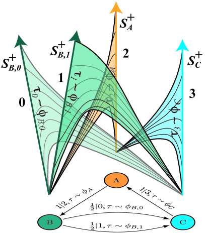
Figure 2: Continuous-time $\epsilon$-machine for the hidden semi-Markov process generated by the uHSMM of Figure 1, as determined by Theorem 1. Continuous-time causal states $\mathcal{S}_{A}^{+}$, $\mathcal{S}_{B}^{+}$, and $\mathcal{S}_{C}^{+}$ track the times $\tau_{0}$ or $\tau_{1}$ since last event—the times obeying distributions $\phi_{A}$, $\phi_{B,0}$, $\phi_{B,1}$, and $\phi_{C}$ associated with uHMM states $A$, $B$, and $C$, respectively. Each renewal subprocess is depicted as a semi-infinite vertical line and is isomorphic with the positive real line. If no event is seen, probability flows towards increasing time since last event, as described in Eq. (8). Otherwise, the surfaces leaving $\mathcal{S}_{A}^{+}$, $\mathcal{S}_{B}^{+}$, and $\mathcal{S}_{C}^{+}$ indicate allowed transitions back to the next reset state or $0$ node located at the non-arrow end, denoting that a new event occurred associated with the next state $A$, $B$, and $C$, as appropriate. Note that when leaving state $B$ there are two distinct diffusion processes on $\mathcal{S}_{B}^{+}$ associated with emitting either $0$ and $1$. The domains of these diffusions are depicted with two separate semi-infinite lines, denoted $\mathcal{S}_{B,0}^{+}$ and $\mathcal{S}_{B,1}^{+}$, respectively. Figure 1’s generative HSMM is displayed underneath for reference.

A process’ statistical complexity is defined as the entropy of its causal states. To calculate this, we need to find the probability distribution over the triple $(g_{0},x_{0^{+}},\tau_{0^{+}})$. After some straightforward calculation, we find the statistical complexity as stated in Proposition 1.

Proposition 1.

The statistical complexity of a unifilar hidden semi-Markov process, under weak assumptions, is given by:

$$C_{\mu}=\operatorname{H}[p(g)]-\sum_{g}p(g)\left(\sum_{x}T^{(x)}_{g}\log T_{g}^{(x)}\right)-\sum_{g}p(g)\int_{0}^{\infty}\left(\mu_{g}\Phi_{g}(\tau)\right)\log\left(\mu_{g}\Phi_{g}(\tau)\right)d\tau~{},$$

where, as above, $p(g)$ is the normalized right eigenvector of eigenvalue $1$ of the matrix of Eq. (8).

Proof.

Altogether, we find that the statistical complexity is:

$$C_{\mu} =\operatorname{H}[\mathcal{G},X,\mathcal{T}]$$

$$=\operatorname{H}[\mathcal{G}]+\operatorname{H}[X|\mathcal{G}]+\operatorname{H}[\mathcal{T}|\mathcal{G},X]$$

$$=\operatorname{H}[p(g)]-\sum_{g}p(g)\left(\sum_{x}T^{(x)}_{g}\log T_{g}^{(x)}\right)-\sum_{g}p(g)\int_{0}^{\infty}\left(\mu_{g}\Phi_{g}(\tau)\right)\log\left(\mu_{g}\Phi_{g}(\tau)\right)d\tau,$$

where $p(g)$ is given above.

As with continuous-time renewal processes, this is the statistical complexity of a mixed random variable and, hence, is not always an upper bound on the excess entropy ${\bf E}:=\operatorname{I}\bigg{[}\smash{\overleftarrow{(X,\mathcal{T})}};\smash{\overrightarrow{(X,\mathcal{T})}}\bigg{]}$.

IV Informational architecture

Finally, we use the causal-state identification to calculate a uHSMP’s entropy rate. Entropy rates are defined via:

$$h_{\mu}=\lim_{T\rightarrow\infty}\frac{\operatorname{H}\big{[}\smash{\overrightarrow{(X,\mathcal{T})}}^{T}\big{]}}{T}~{},$$

but can be calculated using:

$$h_{\mu}=\lim_{\delta\rightarrow 0}\frac{\operatorname{H}\big{[}\smash{\overrightarrow{(X,\mathcal{T})}}^{\delta}\big{|}\smash{\overleftarrow{(X,\mathcal{T})}}\big{]}}{\delta}~{}.$$

Starting there and recalling the definition of causal states, we immediately have:

$$h_{\mu}=\lim_{\delta\rightarrow 0}\frac{\operatorname{H}\big{[}\smash{\overrightarrow{(X,\mathcal{T})}}^{\delta}\big{|}\mathcal{S}\big{]}}{\delta}~{}.$$ (9)

After a little contemplation, we find that entropy rate is as stated in Theorem 2.

Theorem 2.

The entropy rate of a unifilar hidden semi-Markov process is given by:

$$h_{\mu}=-\sum_{g}p(g)\int_{0}^{\infty}\mu_{g}\phi_{g}(\tau)\log\phi_{g}(\tau)d\tau~{},$$

where, as above, $p(g)$ is the normalized right eigenvector associated with eigenvalue $1$ of the matrix in Eq. (8).

Proof.

As just noted, the entropy rate can be calculated via:

$$h_{\mu}=\lim_{\delta\rightarrow 0}\frac{\operatorname{H}\big{[}\smash{\overrightarrow{(X,\mathcal{T})}}^{\delta}\big{|}\mathcal{S}\big{]}}{\delta}~{},$$

where $\smash{\overrightarrow{(X,\mathcal{T})}}^{\delta}$ are trajectories of time length $\delta$. Following Ref. [23], we consider the random variable $X_{\delta}$ to be $0$ when emitted symbol is constant throughout the trajectory of length $\delta$, $1$ when there is one switch from one emitted symbol to another in this trajectory of length $\delta$, and so on. Basic formulae give:

$$\operatorname{H}\big{[}\smash{\overrightarrow{(X,\mathcal{T})}}^{\delta}\big{|}\mathcal{S}\big{]}=\operatorname{H}[X_{\delta}|\mathcal{S}]+\operatorname{H}\big{[}\smash{\overrightarrow{(X,\mathcal{T})}}^{\delta}\big{|}X_{\delta},\mathcal{S}\big{]}~{}.$$ (10)

The key reason that we condition on $X_{\delta}$ is that two switches are highly unlikely to happen relative to one switch. Furthermore, if no switches in emitted symbols occur, then the trajectory is entirely predictable and does not contribute to the entropy rate. In particular:

$$\Pr(X_{\delta}=1|\mathcal{S}=(g,x,\tau)) =\int_{0}^{\delta}\frac{\phi_{g}(\tau+s)}{\Phi_{g}(\tau+s)}ds$$

$$\approx\frac{\phi_{g}(\tau)}{\Phi_{g}(\tau)}\delta+O(\delta^{2})~{}\text{and}$$

$$\Pr(X_{\delta}=k|\mathcal{S}=(g,x,\tau)) =O(\delta^{k})$$

and so:

$$\Pr(X_{\delta}=0|\mathcal{S}=(g,x,\tau)) =1-\Pr(X_{\delta}\geq 1|\mathcal{S}=(g,x,\tau))$$

$$=1-\frac{\phi_{g}(\tau)}{\Phi_{g}(\tau)}\delta+O(\delta^{2})~{}.$$

In a straightforward way, it follows that:

$$\operatorname{H}[X_{\delta}|\mathcal{S}=(g,x,\tau)] =-\left(1-\frac{\phi_{g}(\tau)}{\Phi_{g}(\tau)}\delta\right)\log\left(1-\frac{\phi_{g}(\tau)}{\Phi_{g}(\tau)}\delta\right)-\left(\frac{\phi_{g}(\tau)}{\Phi_{g}(\tau)}\delta\right)\log\left(\frac{\phi_{g}(\tau)}{\Phi_{g}(\tau)}\delta\right)+O(\delta^{2}\log\delta)$$

$$=\frac{\phi_{g}(\tau)}{\Phi_{g}(\tau)}\delta-\left(\frac{\phi_{g}(\tau)}{\Phi_{g}(\tau)}\log\frac{\phi_{g}(\tau)}{\Phi_{g}(\tau)}\right)\delta-\frac{\phi_{g}(\tau)}{\Phi_{g}(\tau)}\delta\log\delta+O(\delta^{2}\log\delta)~{},$$ (11)

after several Taylor approximations; e.g., $\log(1+x)=x+O(x^{2})$.

Now, consider the second term in Eq. (10):

$$\operatorname{H}\big{[}\smash{\overrightarrow{(X,\mathcal{T})}}^{\delta}\big{|}X_{\delta},\mathcal{S}=(g,x,\tau)\big{]} =\Pr(X_{\delta}=0|\mathcal{S}=(g,x,\tau))\operatorname{H}\big{[}\smash{\overrightarrow{(X,\mathcal{T})}}^{\delta}\big{|}X_{\delta}=0,\mathcal{S}=(g,x,\tau)\big{]}$$

$$\qquad+\Pr(X_{\delta}=1|\mathcal{S}=(g,x,\tau))\operatorname{H}\big{[}\smash{\overrightarrow{(X,\mathcal{T})}}^{\delta}\big{|}X_{\delta}=1,\mathcal{S}=(g,x,\tau)\big{]}$$

$$\qquad+\sum_{k=2}^{\infty}P(X_{\delta}=k|\mathcal{S}=(g,x,\tau))\operatorname{H}\big{[}\smash{\overrightarrow{(X,\mathcal{T})}}^{\delta}\big{|}X_{\delta}=k,\mathcal{S}=(g,x,\tau)\big{]}~{}.$$

If $X_{\delta}=0$, the trajectory is completely determined by $\mathcal{S}=(g,x,\tau)$, and hence

$$\operatorname{H}\big{[}\smash{\overrightarrow{(X,\mathcal{T})}}^{\delta}\big{|}X_{\delta}=0,\mathcal{S}=(g,x,\tau)\big{]}=0~{}.$$

If $X_{\delta}=1$, then the trajectory is completely determined by one time—that at which emitted symbols switch. As in Ref. [23], the distribution of switching time is roughly uniform over the interval, and so:

$$\operatorname{H}\big{[}\smash{\overrightarrow{(X,\mathcal{T})}}^{\delta}\big{|}X_{\delta}=1,\mathcal{S}=(g,x,\tau)\big{]}=\log\delta+O(\delta)~{}.$$

Finally, from maximum entropy arguments:

$$P(X_{\delta}=k|\mathcal{S}=(g,x,\tau))\operatorname{H}\big{[}\smash{\overrightarrow{(X,\mathcal{T})}}^{\delta}\big{|}X_{\delta}=k,\mathcal{S}=(g,x,\tau)\big{]}$$

is at most of $\delta^{k}(\log\delta)^{k}$. In particular, we noted earlier that $P(X_{\delta}=k|\mathcal{S}=(g,x,\tau))$ was $O(\delta^{k})$ and that $k$ emissions over a time interval of no more than $\delta$ yields differential entropy of no more than $(\log\delta)^{k}$. In addition, we have:

$$\operatorname{H}\big{[}\smash{\overrightarrow{(X,\mathcal{T})}}^{\delta}\big{|}X_{\delta}=k\big{]}\geq\operatorname{H}\big{[}\smash{\overrightarrow{(X,\mathcal{T})}}^{\delta}\big{|}X_{\delta}=1\big{]}~{}.$$

That is, if given a trajectory with a single transition, one can construct trajectories that approximate it arbitrarily closely with more than one transition. And so, $\big{|}\operatorname{H}\big{[}\smash{\overrightarrow{(X,\mathcal{T})}}^{\delta}\big{|}X_{\delta}=k\big{]}\big{|}$ is at least $O(|\log\delta|)$ and at most $O(|\log\delta|^{k})$. Hence:

$$\sum_{k=2}^{\infty}P(X_{\delta}=k|\mathcal{S}=(g,x,\tau))\operatorname{H}\big{[}\smash{\overrightarrow{(X,\mathcal{T})}}^{\delta}\big{|}X_{\delta}=k,\mathcal{S}=(g,x,\tau)\big{]}=O(\delta^{2}(\log\delta)^{2})~{}.$$

Altogether, we have:

$$\operatorname{H}[\smash{\overrightarrow{(X,\mathcal{T})}}^{\delta}|\mathcal{S}=(g,x,\tau)] =\frac{\phi_{g}(\tau)}{\Phi_{g}(\tau)}\delta-\left(\frac{\phi_{g}(\tau)}{\Phi_{g}(\tau)}\log\frac{\phi_{g}(\tau)}{\Phi_{g}(\tau)}\right)\delta-\frac{\phi_{g}(\tau)}{\Phi_{g}(\tau)}\delta\log\delta+\frac{\phi_{g}(\tau)}{\Phi_{g}(\tau)}\delta\log\delta+O(\delta^{2}(\log\delta)^{2})$$

$$=\frac{\phi_{g}(\tau)}{\Phi_{g}(\tau)}\delta-\left(\frac{\phi_{g}(\tau)}{\Phi_{g}(\tau)}\log\frac{\phi_{g}(\tau)}{\Phi_{g}(\tau)}\right)\delta+O(\delta^{2}(\log\delta)^{2})$$

and, thus:

$$\operatorname{H}[\smash{\overrightarrow{(X,\mathcal{T})}}^{\delta}|\mathcal{S}] =\left\langle\operatorname{H}\big{[}\smash{\overrightarrow{(X,\mathcal{T})}}^{\delta}\big{|}\mathcal{S}=(g,x,\tau)\big{]}\right\rangle_{g,x,\tau}$$

$$=\left\langle\frac{\phi_{g}(\tau)}{\Phi_{g}(\tau)}-\frac{\phi_{g}(\tau)}{\Phi_{g}(\tau)}\log\frac{\phi_{g}(\tau)}{\Phi_{g}(\tau)}\right\rangle_{g,x,\tau}\delta+O(\delta^{2}(\log\delta)^{2})~{}.$$

And so, from Eq. (9), we find the entropy rate:

$$h_{\mu} =\lim_{\delta\rightarrow\infty}\frac{\operatorname{H}\big{[}\smash{\overrightarrow{(X,\mathcal{T})}}^{\delta}\big{|}\mathcal{S}\big{]}}{\delta}$$

$$=\left\langle\frac{\phi_{g}(\tau)}{\Phi_{g}(\tau)}-\frac{\phi_{g}(\tau)}{\Phi_{g}(\tau)}\log\frac{\phi_{g}(\tau)}{\Phi_{g}(\tau)}\right\rangle_{g,x,\tau}$$

$$=\sum_{g,x}p(g)T^{(x)}_{g}\int_{0}^{\infty}\mu_{g}\Phi_{g}(\tau)\frac{\phi_{g}(\tau)}{\Phi_{g}(\tau)}d\tau-\sum_{g,x}p(g)T^{(x)}_{g}\int_{0}^{\infty}\mu_{g}\Phi_{g}(\tau)\frac{\phi_{g}(\tau)}{\Phi_{g}(\tau)}\log\frac{\phi_{g}(\tau)}{\Phi_{g}(\tau)}$$

$$=\sum_{g,x}p(g)T^{(x)}_{g}\left(\int_{0}^{\infty}\mu_{g}\phi_{g}(\tau)d\tau-\int_{0}^{\infty}\mu_{g}\phi_{g}(\tau)\log\frac{\phi_{g}(\tau)}{\Phi_{g}(\tau)}d\tau\right)~{}.$$

We directly have:

$$\int_{0}^{\infty}\mu_{g}\phi_{g}(\tau)d\tau=\mu_{g}$$

and:

$$\int_{0}^{\infty}\mu_{g}\phi_{g}(\tau)\log\frac{\phi_{g}(\tau)}{\Phi_{g}(\tau)} =\int_{0}^{\infty}\mu_{g}\phi_{g}(\tau)\log\phi_{g}(\tau)d\tau-\int_{0}^{\infty}\mu_{g}\phi_{g}(\tau)\log\Phi_{g}(\tau)d\tau~{}.$$

The second term simplifies substituting $u=\Phi_{g}(\tau)$:

$$\int_{0}^{\infty}\mu_{g}\phi_{g}(\tau)\log\Phi_{g}(\tau)d\tau =-\int_{1}^{0}\mu_{g}\log udu$$

$$=\mu_{g}\left(u\log u-u\right)|_{0}^{1}$$

$$=-\mu_{g}~{}.$$

Altogether, we find:

$$h_{\mu}=-\sum_{g}p(g)\int_{0}^{\infty}\mu_{g}\phi_{g}(\tau)\log\phi_{g}(\tau)d\tau~{}.$$

Theorem 2 easily generalizes a recent theorem about the entropy rate of semi-Markov processes [22] to, essentially, hidden semi-Markov processes. In other words, Theorem 2 demonstrates the power of causal-state identification.

V Conclusion

Proposition 1 and Theorem 2 provide new plug-in estimators for the statistical complexity and entropy rate, respectively, of continuous-time, discrete-event processes. It might seem that using these expressions requires an accurate estimation of $\phi_{g}(\tau)$, which then might require unreasonable amounts of data. However, a method first utilized by Lovchenko and popularized by Victor [24] utilizes the fact that we need only calculate scalar functions of $\phi_{g}(\tau)$ and not $\phi_{g}(\tau)$ itself. A second concern arises from the super-exponential explosion of discrete-time, discrete-alphabet $\epsilon$-machines with the number of hidden states [25]. How do we know the underlying topology? Here, we suggest taking the approach of Ref. [26], replacing the hidden states in these general models with the last $k$ symbols. Further research is required, though, to determine when the chosen $k$ is too small or too large.

- [1] C. E. Shannon. A mathematical theory of communication. Bell Sys. Tech. J., 27:379–423, 623–656, 1948.
- [2] J. P. Crutchfield and K. Young. Inferring statistical complexity. Phys. Rev. Let., 63:105–108, 1989.
- [3] C. R. Shalizi and J. P. Crutchfield. Computational mechanics: Pattern and prediction, structure and simplicity. J. Stat. Phys., 104:817–879, 2001.
- [4] A. N. Kolmogorov. Foundations of the Theory of Probability. Chelsea Publishing Company, New York, second edition, 1956.
- [5] G. Chaitin. On the length of programs for computing finite binary sequences. J. ACM, 13:145, 1966.
- [6] J. P. Crutchfield. Between order and chaos. Nature Physics, 8(January):17–24, 2012.
- [7] D. P. Varn and J. P. Crutchfield. Chaotic crystallography: How the physics of information reveals structural order in materials. Curr. Opin. Chem. Eng., 7:47–56, 2015.
- [8] D. Kelly, M. Dillingham, A. Hudson, and K. Wiesner. A new method for inferring hidden Markov models from noisy time sequences. PLoS One, 7(1):e29703, 01 2012.
- [9] C.-B. Li, H. Yang, and T. Komatsuzaki. Multiscale complex network of protein conformational fluctuations in single-molecule time series. Proc. Natl. Acad. Sci. USA, 105:536–541, 2008.
- [10] C.-B. Li and T. Komatsuzaki. Aggregated Markov model using time series of a single molecule dwell times with a minimum of excessive information. Phys. Rev. Lett., 111:058301, 2013.
- [11] S. Marzen, M. R. DeWeese, and J. P. Crutchfield. Time resolution dependence of information measures for spiking neurons: Scaling and universality. Front. Comput. Neurosci., 9:109, 2015.
- [12] M. C. Gonzalez, C. A. Hidalgo, and A.-L. Barabasi. Understanding individual human mobility patterns. Nature, 453(7196):779–782, 2008.
- [13] A. Witt, A. Neiman, and J. Kurths. Characterizing the dynamics of stochastic bistable systems by measures of complexity. Physical Review E, 55:5050–5059, 1997.
- [14] R. W. Clarke, M. P. Freeman, and N. W. Watkins. Application of computational mechanics to the analysis of natural data: An example in geomagnetism. Phys. Rev. E, 67:016203, 2003.
- [15] M. Dzugutov, E. Aurell, and A. Vulpiani. Universal relation between the Kolmogorov-Sinai entropy and the thermodynamical entropy in simple liquids. Phys. Rev. Let., 81:1762, 1998.
- [16] W. M. Gonçalves, R. D. Pinto, J. C. Sartorelli, and M. J. de Oliveira. Inferring statistical complexity in the dripping faucet experiment. Physica A, 257(1-4):385–389, 1998.
- [17] A. Jay Palmer, C. W. Fairall, and W. A. Brewer. Complexity in the atmosphere. IEEE Trans. Geosci. Remote Sens., 38:2056–2063, 2000.
- [18] R. T. Cerbus and W. I. Goldburg. Information content of turbulence. Phys. Rev. E, 88:053012, 2013.
- [19] T. Akimoto, T. Hasumi, and Y. Aizawa. Characterization of intermittency in renewal processes: Application to earthquakes. Phys. Rev. E, 81:031133, 2010.
- [20] R. W. Clarke, M. P. Freeman, and N. W. Watkins. The application of computational mechanics to the analysis of geomagnetic data. Phys. Rev. E, 67:160–203, 2003.
- [21] D. Darmon, J. Sylvester, M. Girvan, and W. Rand. Predictability of user behavior in social media: Bottom-up versus top-down modeling. arXiv.org:1306.6111.
- [22] V. Girardin. On the different extensions of the ergodic theorem of information theory. In R. Baeza-Yates, J. Glaz, H. Gzyl, J. Husler, and J. L. Palacios, editors, Recent Advances in Applied Probability Theory, pages 163–179. Springer US, 2005.
- [23] S. Marzen and J. P. Crutchfield. Complexity and randomness of continuous-time, discrete-event processes. J. Stat. Phys., in press, 2017. arXiv.org:1611.01099.
- [24] Jonathan D Victor. Binless strategies for estimation of information from neural data. Phys. Rev. E, 66(5):051903, 2002.
- [25] B. D. Johnson, J. P. Crutchfield, C. J. Ellison, and C. S. McTague. Enumerating finitary processes. page submitted, 2012. arXiv.org:1011.0036.
- [26] C. C. Strelioff, J. P. Crutchfield, and Alfred Hübler. Inferring Markov chains: Bayesian estimation, model comparison, entropy rate, and out-of-class modeling. Phys. Rev. E, 76(1):011106, 2007.