Comparison of forcing functions in magnetohydrodynamics

Abstract

Results are presented of direct numerical simulations of incompressible, homogeneous magnetohydrodynamic turbulence without a mean magnetic field, subject to different mechanical forcing functions commonly used in the literature. Specifically, the forces are negative damping (which uses the large-scale velocity field as a forcing function), a nonhelical random force, and a nonhelical static sinusoidal force (analogous to helical ABC forcing). The time evolution of the three ideal invariants (energy, magnetic helicity and cross helicity), the time-averaged energy spectra, the energy ratios and the dissipation ratios are examined. All three forcing functions produce qualitatively similar steady states with regards to the time evolution of the energy and magnetic helicity. However, differences in the cross helicity evolution are observed, particularly in the case of the static sinusoidal method of energy injection. Indeed, an ensemble of sinusoidally-forced simulations with identical parameters shows significant variations in the cross helicity over long time periods, casting some doubt on the validity of the principle of ergodicity in systems in which the injection of helicity cannot be controlled. Cross helicity can unexpectedly enter the system through the forcing function and must be carefully monitored.

I Introduction

Turbulence is a diverse and complex phenomenon that has been a source of interest for 100 years, if not more, and from many different disciplines. The Navier-Stokes equations that describe the turbulent flow of a nonconducting fluid are well-known but their nonlinear nature prohibits a complete understanding of them. To describe the behavior of conducting fluids, they are combined with Maxwell’s equations of electromagnetism to form the magnetohydrodynamic equations. These equations can be applied to many astrophysical and geophysical flows, and they also have industrial applications Biskamp2003 ; Davidson2001 ; Frisch1995 ; Verma2004 .

The advent of high performance computing has caused a rapid growth in the study of turbulence. Direct numerical simulations (DNS) are a computationally expensive tool that allows us to follow the exact evolution of a turbulent flow without introducing any modeling. However, it is often useful to inject energy into a turbulent system to compensate for the energy lost through dissipation, and in these forced simulations, a decision has to be made about the method of energy injection. Once a balance is achieved between the energy lost and the energy injected, the system’s statistical properties can be studied. Homogeneous turbulence, which allows fundamental aspects of turbulence to be studied without concern for additional effects from, e.g., boundary conditions, is often simulated. Strictly speaking, an infinite domain is required for homogeneous turbulence but in computational studies this is replaced by periodic boundary conditions.

A wide range of approaches to forcing homogeneous turbulence simulations has been used over the years. Most often these involve injecting energy into the smallest wavenumbers, with or without introducing some random component, see e.g. Refs. Eswaran1988 ; Alvelius1999 ; Zeren2010 . Different forcing methods have different advantages. A deterministic force could be seen as more physical but stochastic forces may provide better control over energy and helicity input. Another example is that a deterministic forcing may produce fluctuations on larger time scales than a stochastic forcing and so it may require a longer run-time to obtain converged statistics, despite being more efficient computationally Zeren2010 .

At the core of the study of homogeneous isotropic turbulence are the contributions of Richardson, Kolmogorov and Obukhov, which include the energy cascade (the notion that energy is transferred from large scales to progressively smaller scales where dissipation dominates), the self-similar scaling of structure functions and the famous ‘five-thirds’ power law for the energy spectrum, $E(k)\propto k^{-5/3}$. These features give rise to the concept of universality in nonconducting fluids, which is the idea that the small-scale evolution of a turbulent system is independent of the large-scale features, such as geometry or the method of energy injection. The concept of universality has been supported by many experiments, numerical simulations and theoretical arguments since then McComb2014 ; Batchelor1953 ; Frisch1995 ; Pope2000 .

Universality in magnetohydrodynamics (MHD) is questionable; highlighted especially by the unusual presence of an inverse cascade of magnetic helicity under certain conditions, which causes some energy to be transferred to the large scales Leorat1975 ; Pouquet1976 ; Alexakis2005a ; Alexakis2007 . The three ideal invariants in MHD are the total energy, magnetic helicity and cross helicity. The latter two quantities represent the knottedness of magnetic field lines and the alignment of the velocity and magnetic fields Moffat1969 . It is known that these parameters can alter aspects of MHD systems such as the (dimensionless) dissipation rate Linkmann2015 ; Linkmann2017 ; Dallas2013 . This comes as a result of selective decay processes, that is, the tendency for the fields to self-organize into a force-free state in which the magnetic helicity is maximal, or an Alfvénic state in which the velocity and magnetic fields are fully aligned Biskamp2003 ; Dobrowolny1980 . The alignment of the fields weakens the turbulence, slowing down the decay of energy in unforced systems Biskamp2003 ; Stribling1991 . Furthermore, the presence or absence of a background magnetic field affects the turbulent dynamics, and this is reflected in the scaling of the energy spectrum. In forced MHD with a strong background magnetic field, the theory of dynamic alignment predicts the field-perpendicular energy scaling $E(k_{\perp})\propto k^{-3/2}$ Boldyrev2006 . This comes as a result of the tendency for the magnetic and velocity fluctuations to become aligned, with a more pronounced effect at smaller scales. However, dynamic alignment may also occur at small scales in the absence of a guide field, since large-scale magnetic-field fluctuations can play a similar role for small-scale fluctuations as the guide field Boldyrev2006 .

Interestingly, it was found that self-organised states can be obtained when both fields are forced in a nonhelical way, depending on the time-correlation of the forcing Dallas2015 . The less often the phase was randomised, the more the cross helicity and magnetic helicity would build up, leading to self-organisation. The Archontis dynamo, in which the velocity field is forced in a nonhelical way, is also known to introduce large values of cross helicity. Furthermore, in the case in which the magnetic and kinetic Reynolds numbers Rm and Re are equal, the Archontis dynamo saturates with the magnetic and kinetic energy almost in equipartition Archontis2007 ; Dorch2004 ; Gilbert2011 ; Cameron2006 . It is important to be sure that effects such as these are independent of the specific implementation of the forcing, especially since MHD has many cosmological, astrophysical and industrial applications and relies heavily on results from numerical simulations. The importance of understanding how independent the turbulence properties are of the forcing function has been underpinned by the above discussion.

In this paper, we present a systematic study that examines the effect of different forcing functions in MHD. We investigate the evolution of homogeneous, incompressible MHD turbulence without a mean magnetic field, subject to three different types of mechanical forcing functions that aim to represent the range of forcing methods used in the literature. Specifically, we use (i) a mechanical force that uses the large-scale velocity field as a forcing function, (ii) a nonhelical random force defined by using time-varying helical basis vectors, and (iii) a nonhelical static sinusoidal force. In Sec. II we give details of our simulations, including the three forcing routines. In Sec. III we examine the time evolution of the three ideal invariants (energy, magnetic helicity and cross helicity), the time-averaged energy and cross helicity spectra, the energy ratios and the dissipation ratios. As we will show, the magnetic helicity remains close to zero in all cases but the sinusoidal method of energy injection has a tendency to introduce cross helicity into the system. Indeed, our results for sinusoidally-forced simulations with identical parameters and different initial conditions show large variations in the normalised cross helicity over long time periods. We discuss these results in Sec. IV and draw some conclusions.

II Numerical method

Run ID	Type	$N$	$\nu$	Re	$\text{Re}_{\lambda}$	$k_{max}/k_{\eta}$	$k_{max}/k_{\nu}$	$\rho_{b}$	$\rho_{u}$	$\rho_{c}$	$\sigma_{c}$
AHFa	AHF	1024	0.000625	1085	218	2.49	3.13	-0.00011	0.0014	-0.012	-0.010
NDa	ND	1024	0.000625	1293	233	2.60	3.26	0.0036	0.040	0.063	0.057
SFa	SF	1024	0.000625	1524	272	2.61	3.27	0.016	-0.0034	0.10	0.084
AHFb	AHF	512	0.0008	742	180	1.50	1.88	0.0077	0.00063	0.026	0.023
NDb	ND	512	0.0008	994	213	1.56	1.96	-0.0043	0.045	-0.035	-0.030
SFb	SF	512	0.0008	1190	236	1.55	1.94	-0.0046	0.0027	-0.16	-0.13
AHFc	AHF	512	0.001	609	162	1.77	2.20	-0.0038	-0.0072	0.012	0.010
NDc	ND	512	0.001	803	179	1.85	2.28	-0.029	-0.00015	0.22	0.21
SFc	SF	512	0.001	940	207	1.85	2.31	0.0022	0.00076	-0.012	-0.010
AHFd	AHF	256	0.0015	374	125	1.25	1.51	-0.0039	0.0037	-0.0084	-0.0069
NDd	ND	256	0.0015	535	152	1.25	1.53	-0.0046	0.044	-0.093	-0.080
SFd	SF	256	0.0015	618	164	1.25	1.55	0.011	-0.0046	-0.029	-0.025
AHFe	AHF	256	0.002	308	113	1.55	1.82	0.0069	-0.0098	-0.0062	-0.0049
NDe	ND	256	0.002	410	134	1.56	1.88	-0.013	0.059	0.0010	0.00081
SFe	SF	256	0.002	541	161	1.45	1.76	-0.0037	0.0015	0.013	0.010
AHFf	AHF	128	0.005	127	62	1.61	1.61	-0.0044	-0.0019	-0.0088	-0.0060
NDf	ND	128	0.005	171	76	1.58	1.72	0.0036	-0.041	0.024	0.018
SFf	SF	128	0.005	211	89	1.46	1.65	0.021	-0.014	0.10	0.080

Table 1: Table of basic parameters including the forcing type, number of grid points $N^{3}$, viscosity $\nu$, integral-scale and Taylor-scale Reynolds numbers Re and Re_λ respectively, resolution $k_{max}/k_{\eta}$ and $k_{max}/k_{\nu}$ defined with respect to the magnetic and velocity fields, relative magnetic helicity $\rho_{b}$, relative kinetic helicity $\rho_{u}$, and two definitions of relative cross helicity $\rho_{c}$ and $\sigma_{c}$ (Eqs. (5) and (6)). The values were time-averaged over the duration of the steady state. AHF denotes adjustable helicity forcing, ND denotes negative damping, and SF denotes sinusoidal forcing.

We performed direct numerical simulations of the incompressible MHD equations

$$\partial_{t}{\bm{u}}=-\nabla P-({\bm{u}}\cdot\nabla){\bm{u}}+(\nabla\times{\bm{b}})\times{\bm{b}}+\nu\nabla^{2}{\bm{u}}+{\bm{f}}$$ (1)

$$\partial_{t}{\bm{b}}=\nabla\times({\bm{u}}\times{\bm{b}})+\eta\nabla^{2}{\bm{b}}$$ (2)

$$\nabla\cdot{\bm{u}}=0\text{, }\nabla\cdot{\bm{b}}=0\ ,$$ (3)

where ${\bm{u}}$ is the velocity field, ${\bm{b}}$ is the magnetic field in Alfvén units, $P$ is the pressure, $\nu$ is the kinematic viscosity, $\eta$ is the magnetic diffusivity, and ${\bm{f}}$ is an external force that we will define later. The density was set to unity. We use a caret to denote the Fourier transform of a field. We solved these equations numerically using a pseudospectral, fully-dealiased code (see Yoffe2012 ; Linkmann2016 for details) on a three-dimensional periodic domain with lattice sizes varying from $128^{3}$ to $1024^{3}$ points (see Tab. 1). The initial fields were random Gaussian with magnetic and kinetic energy spectra of the form $E_{b,u}(k,t=0)=Ak^{4}\exp(−k^{2}/(2k_{0})^{2})$, where A is a positive real number and $k_{0}$ is the peak of the spectrum, which we set to 5 in all cases. There was no imposed magnetic guide field. The simulations were all spatially well-resolved, with the maximum resolved wavenumber always at least 1.25 times greater than the dissipation wavenumbers $k_{\nu}=(\epsilon_{u}/\nu^{3})^{1/4}$ and $k_{\eta}=(\epsilon_{b}/\eta^{3})^{1/4}$ associated with the Kolmogorov microscales, where $\epsilon_{u}$ and $\epsilon_{b}$ are the kinetic and magnetic dissipation rates. For simplicity we limited our study to the case where the magnetic Prandtl number, Pm$=$Rm$/$Re$=\nu/\eta$, is one.

We examined the variations of the relative magnetic helicity and cross helicity. The relative magnetic helicity is defined as

$$\rho_{b}=\langle{\bm{b}}\cdot{\bm{a}}\rangle/(\langle|{\bm{b}}|^{2}\rangle\langle|{\bm{a}}|^{2}\rangle)^{1/2}$$ (4)

where ${\bm{a}}$ is the magnetic vector potential, ${\bm{b}}=\nabla\times{\bm{a}}$, and the angular brackets denote a spatial average.

The relative cross helicity can be quantified in two ways:

$$\rho_{c} =\langle{\bm{u}}\cdot{\bm{b}}\rangle/(\langle|{\bm{u}}|^{2}\rangle\langle|{\bm{b}}|^{2}\rangle)^{1/2}\ \text{and}$$ (5)

$$\sigma_{c} =2\langle{\bm{u}}\cdot{\bm{b}}\rangle/(\langle|{\bm{u}}|^{2}\rangle+\langle|{\bm{b}}|^{2}\rangle)\ .$$ (6)

The former is a measurement of the alignment between the fields, whereas the latter is the ratio of two ideal invariants, namely the cross helicity and the total energy. Together they obey the inequality $|\sigma_{c}|\leq|\rho_{c}|\leq 1$ Grappin1983 ; Pouquet1988 . Both definitions have their merits. Their differences and similarities are explored in Sec. III.2. We focus our attention mostly on the larger of the two, $\rho_{c}$, which is more sensitive to the forcing function.

The relative kinetic helicity is defined as

$$\rho_{u}=\langle{\bm{u}}\cdot\bm{\omega}\rangle/(\langle|{\bm{u}}|^{2}\rangle\langle|\bm{\omega}|^{2}\rangle)^{1/2}\ ,$$ (7)

where $\bm{\omega}=\nabla\times{\bm{u}}$ is the vorticity.

Three types of forcing function were used: negative damping (ND), adjustable helicity forcing (AHF) and sinusoidal forcing (SF) which are defined as follows:

II.1 Negative damping

The negative damping function uses the large-scale velocity field as a forcing function. It was first developed as a way to avoid introducing further randomness into an already random system Machiels1997 and it is commonly used in hydrodynamic simulations Jimenez1993 ; Kaneda2003 ; Kaneda2006 ; McComb2015 ; Linkmann2015a . The function is

$${\bm{{\hat{\bm{f}}}}}({\bm{k}},t)=\begin{cases}\frac{\epsilon_{i}{\bm{{\hat{\bm{u}}}}}({\bm{k}},t)}{2E_{u,k_{f}}(t)},&\text{if }1\leq|{\bm{k}}|\leq k_{f}\\ 0&\text{otherwise,}\end{cases}$$ (8)

where $E_{u,k_{f}}(t)=\int_{1}^{k_{f}}E_{u}(k,t)dk$ is the kinetic energy contained in the forcing range $[1,k_{f}]$ and $\epsilon_{i}$ is an adjustable parameter. The rate of energy injection is $\langle{\bm{u}}\cdot{\bm{f}}\rangle=\int d{\bm{k}}\ {\bm{{\hat{\bm{u}}}}}({\bm{k}})\cdot{\bm{{\hat{\bm{f}}}}}(-{\bm{k}})=\epsilon_{i}$ which will be equal to the mean total dissipation rate $\epsilon=\epsilon_{b}+\epsilon_{u}$ during the steady state. We chose our fields’ initial conditions to have negligible kinetic, magnetic and cross helicity and therefore one might expect the fields to remain nonhelical throughout their evolution, although the actual helicity injection cannot be controlled. The variation of cross helicity in MHD subject to negative damping was explored to some extent in Sahoo2011 . The forcing type has been well-used, but nevertheless, it was recently found that, in hydrodynamics, at low Reynolds numbers, negative damping can induce self-ordering effects due to poor control of kinetic helicity injection McComb2015 ; Linkmann2015a .

II.2 Adjustable helicity forcing

The second type of forcing considered uses a helical basis composed of eigenvectors of the curl operator:

$${\bm{{\hat{\bm{f}}}}}({\bm{k}},t)=\begin{cases}A({\bm{k}}){\bm{e}}_{1}({\bm{k}},t)+B({\bm{k}}){\bm{e}}_{2}({\bm{k}},t),&\text{if }1\leq|{\bm{k}}|\leq k_{f}\\ 0&\text{otherwise,}\end{cases}$$ (9)

where ${\bm{e}}_{1}\cdot{\bm{e}}_{2}^{*}={\bm{e}}_{1}\cdot{\bm{k}}={\bm{e}}_{2}\cdot{\bm{k}}=0$ and ${\bm{e}}_{1}$ and ${\bm{e}}_{2}$ are unit vectors that statisfy $i{\bm{k}}\times{\bm{e}}_{1}=k{\bm{e}}_{1}$ and $i{\bm{k}}\times{\bm{e}}_{2}=-k{\bm{e}}_{2}$. At each forcing time step, for every vector ${\bm{k}}$ with magnitude $1\leq|{\bm{k}}|\leq k_{f}$, a corresponding random perpendicular unit vector is generated and used to construct the helical basis; thus the basis is changed every time the forcing function is called. $A({\bm{k}})$ and $B({\bm{k}})$ are complex parameters that can be adjusted to control the helicity of the forcing Brandenburg2001 . In our simulations we set the kinetic helicity to zero, so the forcing was explicitly nonhelical. This type of forcing has been widely used Malapaka2013 ; Muller2012 ; Biferale2012 ; Brandenburg2001 ; Brandenburg2014 .

II.3 Sinusoidal forcing

The sinusoidal forcing we used is deterministic and nonhelical, implemented in real space:

$${\bm{f}}({\bm{x}}) =C\sum_{k=1}^{k_{f}}\begin{pmatrix}\sin(kz)+\sin(ky)\\ \sin(kx)+\sin(kz)\\ \sin(ky)+\sin(kx)\end{pmatrix}\ ,$$ (10)

where $C$ is an adjustable constant. This forcing type was used in Ref. Dallas2015 . It is a nonhelical analog of the well-known ABC forcing, which is fully helical Galanti1992 ; Galloway2012 ; Mininni2007 ; Childress1970 ; Galloway1984 , and it is similar to the Archontis dynamo, ${\bm{f}}({\bm{x}})=(\sin(z),\sin(x),\sin(y))$ Cameron2006 .

III Results

III.1 Energy evolution

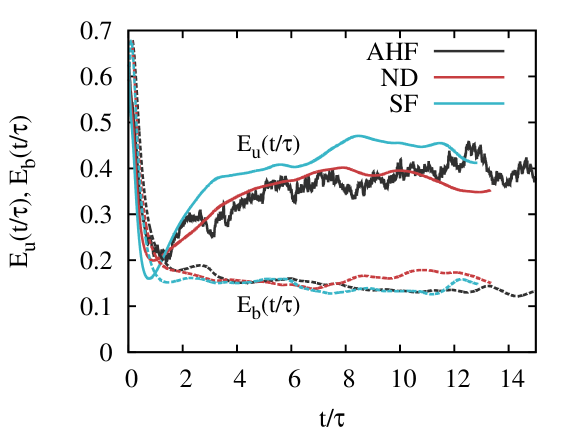
Figure 1: Evolution of kinetic energy (solid lines) and magnetic energy (dashed lines) for runs AHFa, NDa and SFa. $\tau$ is the steady state large eddy turnover time. (Colour online.)

We will describe our results using the $\nu=0.000625$ (AHFa, NDa, and SFa) simulations to demonstrate points, since they attained the highest Reynolds numbers in our tests (see Tab. 1). Using these simulations, which are representative of the other simulations we ran, we will highlight features of the three forcing functions.

Our analysis focuses on various properties of the forced systems while in a statistically steady state. This allows us to look at time-averaged samples of data taken during that period. Figure 1 shows the time evolution of the kinetic and magnetic energies corresponding to runs AHFa, NDa and SFa. An initial transition period precedes the fully-developed statistically steady turbulent state, where the energy injected equals the energy dissipated. We began taking measurements after the transient initial behavior had passed and both the kinetic and magnetic energies were fluctuating around a constant value. The AHF kinetic energy evolution, as seen in Fig. 1, is more erratic than the other two forcing types. This is due to the random nature of the forcing function, as described in Sec. II.2, which causes rapid changes in the amount of energy injected. The time scale was normalized by the steady state large eddy turnover time $\tau=u_{rms}/L$, where $u_{rms}$ is the root-mean-square velocity, $L=3\pi\int_{0}^{\infty}k^{-1}E_{u}(k)dk/(4\int_{0}^{\infty}E_{u}(k)dk)$ is the integral scale and $E_{u}(k)$ is the steady state kinetic energy spectrum. In an isotropic system, $u_{rms}^{2}=\langle u_{i}^{2}\rangle$ for any direction $i$, so the total kinetic energy $E_{u}=3u_{rms}^{2}/2$. All simulations lasted for 100 units of simulation time, corresponding to approximately 30 to 40 large eddy turnover times, except the simulations run on $1024^{3}$ points, which ran for about 40 units of simulation time. The AHF runs generally had a slightly smaller value of $\tau$, meaning that the injected energy was transferred to the smaller scales at a faster rate.

We will use both the integral scale Reynolds number $\text{Re}=u_{rms}L/\nu$ and the Taylor Reynolds number $\text{Re}_{\lambda}=u_{rms}\lambda/\nu$ as metrics to measure the turbulence, since the integral scale Reynolds number is associated with the forcing scales while the Taylor Reynolds number characterizes the turbulence at intermediate scales. Here $\lambda=(15\nu/\epsilon_{u})^{1/2}u_{rms}$ is the Taylor microscale.

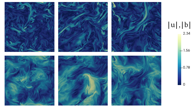
AHFa                                NDa                                SFa

Figure 2: Visualisation of a two-dimensional slice of the magnitudes of the magnetic (top) and velocity (bottom) fields in the AHFa (left), NDa (middle) and SFa (right) cases. (Colour online.)

Two-dimensional slices of the magnitudes of the fields $|{\bm{u}}|$ and $|{\bm{b}}|$ from the AHFa, NDa and SFa simulations at a point in time during the steady state are shown in Fig. 2. These slices are representative of the general structure of the fields throughout the steady state time frame. The time-averaged Reynolds numbers are moderately separated: $\text{Re}=1085,1293$ and $1524$ respectively, but the fields do not differ greatly and exhibit the same level of detail in the small scales. This is to be expected as they have similar dissipation wavenumbers $k_{\eta}$ and $k_{\nu}$ (see Tab. 1). These visualisations demonstrate that, although the forces have very different functional forms, the physical appearance of the fields is similar. Overall we see that all three forces are capable of producing physically-alike steady state behavior in the same time frame.

III.2 Definitions of relative cross helicity

In Sec. II two ways of defining the relative cross helicity were introduced. The time evolution of these quantities and their time-averaged spectra from run SFa are shown in Fig. 3.

As can be seen in the figure, the time evolution of the two metrics follow a similar trajectory, with $\sigma_{c}$ remaining close to, but less than, $\rho_{c}$. The largest separation between $\rho_{c}$ and $\sigma_{c}$ occurs during a period when the difference between the kinetic and magnetic energies was greatest; this effect is apparent from the definitions of $\rho_{c}$ and $\sigma_{c}$ given in Eqs. (5) and (6). When the kinetic and magnetic energies are in equipartition the two quantities coincide.

Figure 3(b) shows the time-averaged cross helicity spectra corresponding to the two definitions in Eqs. (5) and (6)

$$\rho_{c}(k) =\frac{{H_{c}(k)}}{2E_{b}(k)^{1/2}E_{u}(k)^{1/2}}\ ,$$ (11)

$$\sigma_{c}(k) =\frac{{H_{c}(k)}}{E_{b}(k)+E_{u}(k)}\ ,$$ (12)

where $H_{c}(k)=\int_{|{\bm{k}}|=k}d{\bm{k}}\ {\hat{\bm{u}}}({\bm{k}})\cdot{\hat{\bm{b}}}(-{\bm{k}})$ is the cross helicity spectrum. We see that $\rho_{c}(k)$, which is normalised by $2E_{b}(k)^{1/2}E_{u}(k)^{1/2}$, is more sensitive to the ratio of kinetic and magnetic energy than $\sigma_{c}(k)$ is. Because of this, at the forcing scale, where the kinetic energy is much greater than the magnetic energy, the denominator becomes small for $\rho_{c}(k)$ and not for $\sigma_{c}(k)$. Thus $\rho_{c}(k)$ has a large peak that is absent from the $\sigma_{c}(k)$ spectrum. The difference in the low-$k$ relative cross helicity spectra occurs consistently across simulations with different forcing functions. This effect, however, could cause data to be misinterpreted, especially between separate groups of researchers.

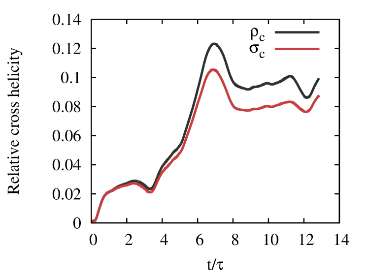
(a)

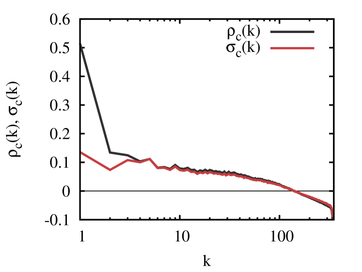
(b)

Figure 3: (a) Time evolution and (b) spectra of the two definitions of relative cross helicity [Eqs. (5) and (6)] for run SFa. Note the logarithmic scale on the $x$-axis in (b). (Colour online.)

III.3 Comparison of energy and cross helicity spectra

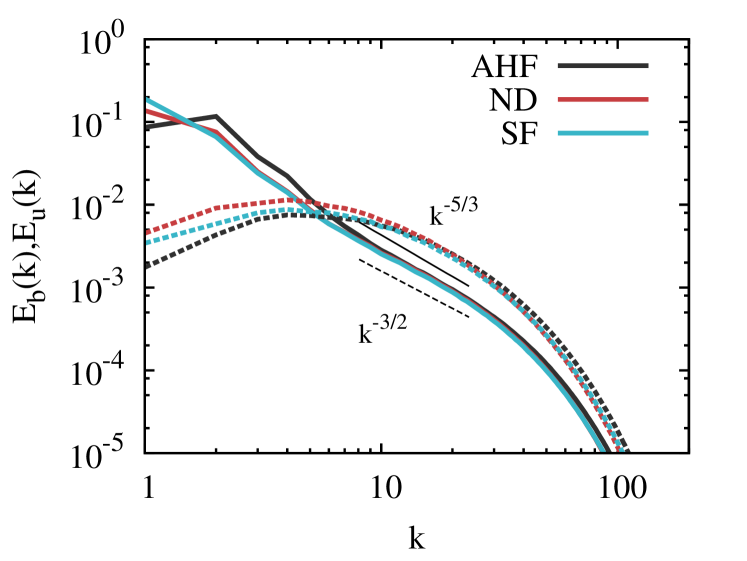
(a)

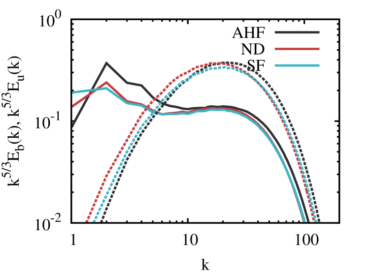
(b)

Figure 4: (a) Kinetic and magnetic energy spectra (solid and dashed lines respectively) and (b) compensated kinetic and magnetic energy spectra for runs AHFa, NDa and SFa. (Colour online.)

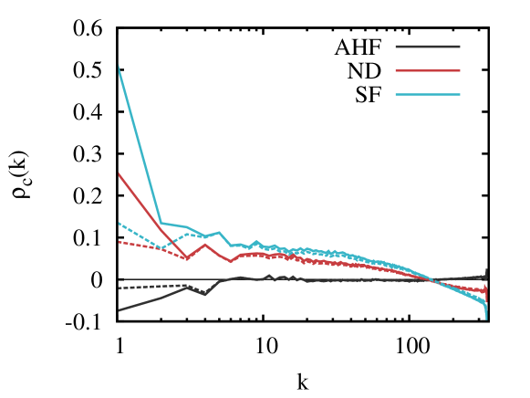
Figure 5: Relative cross helicity spectra for runs AHFa, NDa and SFa. Note the logarithmic scale on the $x$-axis. (Colour online.)

Having identified the onset of the statistically steady state, we can examine the time-averaged energy spectra [Fig. 4(a)]. The spectra coincide in a small inertial subrange but spread out slightly at the large and small scales. All of our simulations had the same low-$k$ behavior, with the ND and SF runs having a peak at $k=1$ and the AHF types peaking at $k=2$.

Both $k^{-5/3}$ and $k^{-3/2}$ scalings have been indicated in Fig. 4(a). The compensated kinetic and magnetic energy spectra are shown in Fig. 4(b). As can be seen in these figures, the power-law range of the kinetic energy spectrum is too short to distinguish between the two scalings. This highlights that we still have to exercise caution in making measurements of this kind, and that larger simulations with a more obvious inertial range are still needed. The inertial range for the magnetic energy spectrum is even less clear. It is plausible that in order to see a clearer scaling we would need to inject energy directly into the magnetic field; this is also indicated by the results of Ref. Alexakis2013 in which the ratio of magnetic to mechanical forcing was varied in generally nonhelical simulations. However, our results focus only on mechanical forcing, as magnetic forcing is known to induce other effects such as large-scale self-organisation Dallas2015 . The runs with smaller Reynolds numbers have steeper energy spectra, presumably because of the enduring problem of the lack of separation between forcing scales and dissipation scales in direct numerical simulations. The steeper slope in the lower range of run AHFa compared to NDa and SFa could thus also be a finite Reynolds number effect, since the adjustable helicity forcing consistently produced simulations with lower Reynolds numbers for a given viscosity.

The turbulence is generated on a discrete Cartesian lattice, so most points do not have integer values of $k$. Instead, a shell-average of points with wavenumbers $n-0.5\leq k<n+0.5$, where $n$ is a positive integer, is used when calculating spectral quantities. This means that sometimes the density of states in a particular shell will be higher or lower than the continuum limit of $4\pi k^{2}$, causing bumps to appear in the spectra. To counteract this, we have taken the spectral energy densities in the $n^{th}$ shell $S_{n}$ to be $E^{n}_{u,b}=\frac{4\pi n^{2}}{M_{n}}\sum_{{\bm{k}}\in S_{n}}E_{u,b}({\bm{k}})$ where $M_{n}$ is the number of wavevectors in the shell Stepanov2014 . This produces a smoother spectrum.

The magnetic and kinetic helicity generally remained negligible (see Table 1), however the cross helicity in some simulations was prone to large fluctuations, yielding time-averaged values of $\rho_{c}$ as large as 0.22 (Run NDc). We have seen that $\rho_{c}(k)$ is peaked at the forcing scales (as shown in Fig. 5) and therefore we conclude that it has been injected by the forcing function. Interestingly, there also tends to be a build-up in the normalised cross helicity at small scales with the opposite sign to the build-up at the large scales.

Due to its effect on the scaling exponents of the energy spectra in MHD in the presence of a magnetic guide field Perez2009 , the behavior of $\sigma_{c}(k)$ has been studied extensively in solar wind data Podesta2010 , numerical simulations Beresnyak2010 and theoretically Podesta2011 . The observational studies found $|\sigma_{c}(k)|$ to be constant in the inertial subrange provided that the average value was large, while states with small mean cross helicity suffered from uncertainties in the measurements.

Here, for steady states with low but non-negligible $\rho_{c}(k)$ and $\sigma_{c}(k)$, we consistently find a tendency to compensate the force-induced alignment between ${\bm{{\hat{\bm{u}}}}}$ and ${\bm{{\hat{\bm{b}}}}}$ at small $k$ (large scales) mostly at large $k$ (small scales). The relative cross helicity at a given scale is related to the scale-dependent alignment angle Boldyrev2006 ; Podesta2010 . However, provided the alignment angle is small, its scale dependence does not enforce a scale dependence of the relative cross helicity Podesta2010 . In view of the aforementioned results on the scale independence of $\sigma_{c}(k)$ for high-cross-helicity states in unbalanced MHD with a guide field, the approximately linear scaling observed here may point to a more complicated situation for low-cross-helicity states, which merits further investigation in its own right. Finally, we do not find a measureable effect of nonzero cross helicity on the scaling of the energy spectra in our data.

III.4 Energy and dissipation ratios

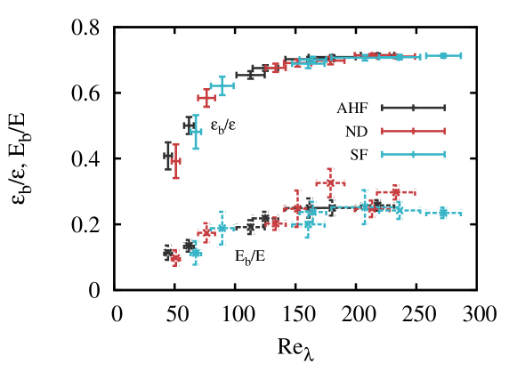
Figure 6: Fraction of magnetic dissipation $\epsilon_{b}/\epsilon$ (plusses) and magnetic energy $E_{b}/E$ (crosses) as a function of Taylor Reynolds number. The error bars are the standard deviation. (Colour online.)

In our tests, only the velocity field was forced and so the magnetic field was sustained through the transfer of kinetic to magnetic energy, i.e., dynamo action. It is useful to know how efficient the nonlinear dynamo is at sustaining its magnetic field, which had initial conditions such that it was in equipartition with the velocity field at $t=0$. Figure 6 shows the ratios $E_{b}/E$ and $\epsilon_{b}/\epsilon$ as a function of the Taylor-scale Reynolds number. The Taylor-scale Reynolds number is used instead of the integral-scale Reynolds number because we are interested in comparing the effects of the forces at smaller scales than the forcing range. The measurements of $E_{b}/E$ and $\epsilon_{b}/\epsilon$ follow a clear trend regardless of the way in which the kinetic energy was injected. In particular, the magnetic dissipation fraction asymptotes quickly to $\epsilon_{b}/\epsilon\simeq 0.71$. This is in agreement with other results for nonhelical simulations with unity magnetic Prandtl number Brandenburg2014 ; Haugen2003 ; Linkmann2017 . The magnetic energy fraction displays slightly more erratic behavior, particularly in run NDc. The scatter is expected because the energy is dominated by the more volatile forcing scales, while the dissipation takes place at small scales. We conclude that the energy transfer and dissipation produced by each type of force are consistent. The efficiency of the nonhelical nonlinear dynamo is independent of the implementation of the large-scale mechanical forcing.

III.5 Injection of ideal invariants

The total energy, magnetic helicity and cross helicity are conserved in the ideal (non-dissipative) limit. It is therefore desirable for the helicities to remain approximately constant during a statistically steady state at high Re and Rm. The total energy in the system fluctuates around a constant value as energy is injected and dissipated and we expect the same from the other two ideal invariants. The initial conditions in our simulations have zero magnetic and cross helicity. The time evolution of relative magnetic helicity and cross helicity is shown in Fig. 7. The mean relative magnetic helicity remains within one standard deviation of zero in all cases, irrespective of the chosen forcing method. This could be expected since the magnetic field is not directly forced and should therefore be less susceptible to large variations.

The relative cross helicity, on the other hand, has the tendency to deviate from zero in some cases, with large fluctuations lasting for long times. This is particularly prevalent in the ND and SF runs, with fluctuations up to $\rho_{c}\simeq 0.3$ at times. Since ND feeds the velocity field back into itself, small fluctuations in cross helicity could be amplified, leading to a runaway effect at large scales. In Fig. 5 we saw that the relative cross helicity is peaked at the forcing scales, so it is clear that the growth of cross helicity is connected to the forcing. To guarantee negligible injection of cross helicity, the alignment between ${\bm{{\hat{\bm{f}}}}}$ and ${\bm{{\hat{\bm{b}}}}}$ (and when a magnetic force ${\bm{f}}_{\bm{b}}$ is present, the alignment between ${\bm{{\hat{\bm{f}}}}}_{\bm{b}}$ and ${\bm{{\hat{\bm{u}}}}}$) should remain negligible. The unusually large fraction of magnetic energy in run NDc, as seen in Fig. 6, could be connected to the presence of high cross helicity. We will come back to this point in the next section.

The influence of intermediate values of cross helicity is not well understood, although it is known that systems with nonzero cross helicity can tend towards an Alfvénic state in which the cross helicity is maximal Grappin1983 . One of the findings of this study that has not been anticipated in the literature is that helicity can unexpectedly enter the system through certain forcing functions. Thus it is of practical importance to monitor and control its injection.

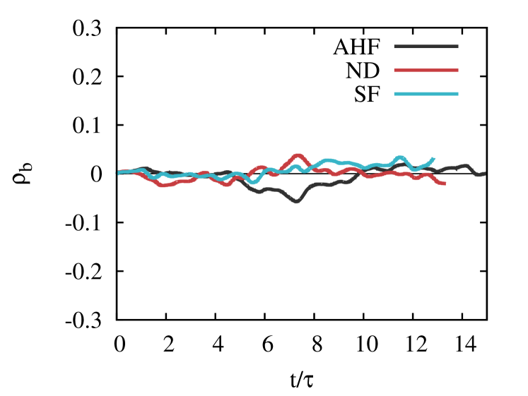
(a)

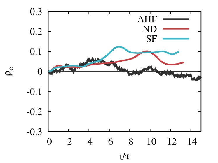
(b)

Figure 7: Evolution of (a) relative magnetic helicity and (b) relative cross helicity for runs AHFa, NDa and SFa. $\tau$ is the time-averaged large eddy turnover time. Note that the y-axis extends to $\pm 0.3$ but the maximum possible values are 1. (Colour online.)

III.6 Comparison of repeated simulations

Generally when using DNS we make the assumption of ergodicity, . e., we assume that in stationary turbulence the time-averaged values from one simulation are equivalent to ensemble-averaged values where the ensemble consists of many simulations. Thus for any set of parameters, usually only one simulation is performed and statistics are obtained by averaging over snapshots in time once the system has reached a steady state. This is the approach we took in the preceeding section. However, we found significant variations in cross helicity over time which prompted us to question how valid the ergodic principle is in situations in which the injection of helicities cannot be controlled. Furthermore, one might expect that the fluctuations of the ideal invariants would decrease as we increase the Reynolds number, since we are increasing the number of interactions at each length scale, but this does not seem to be the case in our tests. Large fluctuations in cross helicity alter the behavior of a flow, for example in Run NDc, which had an average relative cross helicity $\rho_{c}=0.22$ and a larger than expected energy fraction $E_{b}/E$.

To test the variability of the cross helicity and its effect on the distribution of energy between the two fields, we ran an ensemble of 20 simulations for each forcing type on a $128^{3}$ grid with viscosity $\nu=0.008$. The time-averaged Reynolds numbers and relative cross helicity $\rho_{c}$ are shown in Tab. 2. In all cases, the time-averaged Reynolds numbers stayed in a close range. The relative cross helicity, however, was less consistent, particularly in the SF ensembles. We plotted the time evolution of the magnetic energy fraction against the relative cross helicity for all our simulations to explore the possibility of a connection between the two quantities (Fig. 8). We see further evidence of the variability of cross helicity in the SF cases and also what seems to be a tendency for the magnetic energy fraction to increase as the magnitude of cross helicity increases. This observation for fairly low levels of cross helicity is reminiscent of the behavior of the Archontis dynamo, which produces high levels of cross helicity and saturates with the velocity and magnetic fields approximately in equipartition Archontis2007 . Rapid variations in cross helicity have also been observed in MHD shell models subject to a constant mechanical force Frick2000 . Since the SF is static and the AHF is randomised at every time step, the behavior we see also echoes that of Ref. Dallas2015 , who explored the effect of the correlation time of a kinetic and magnetic force on the helicities. Their results showed that the less often the force was randomised, the more the cross helicity was likely to grow. We see a similar effect here, although we only forced the velocity field.

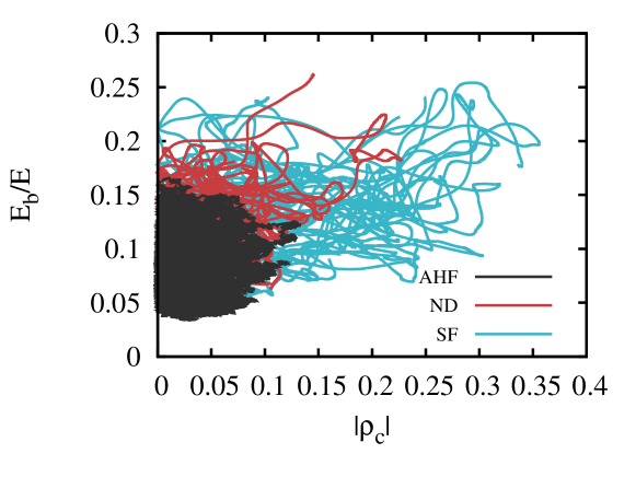
Figure 8: Magnitude of relative cross helicity versus the fraction of magnetic energy $E_{b}/E$ at each point in time of the steady-state ensembles with $\nu=0.008$. (Colour online.)

Type	Re	Reλ	$|\rho_{c}|$	#
AHF	$80-87$	$44-46$	$7.41\times 10^{-6}-0.0256$	20
ND	$100-111$	$52-57$	$0.000686-0.0561$	20
SF	$132-141$	$66-70$	$0.00111-0.193$	20

Table 2: The range of time-averaged quantities (integral-scale Reynolds number Re, Taylor-scale Reynolds number Re_λ and relative cross helicity magnitude $|\rho_{c}|$) from ensembles of each of the three forcing types with $\nu=0.008$ on $128^{3}$ grid points.

The results of this section suggest that the ergodic principle does not hold well when the fluid is subject to the static sinusoidal forcing, as the relative cross helicity can vary significantly from one run to another, which affects aspects of the system such as the energy distribution. This is also likely the case with ND to a lesser degree. The concept of nonuniversality is of interest here, since two simulations with large average values of cross helicity of opposite sign would surely not behave in the same way as a system with zero cross helicity, despite the ensemble-averaged values being small. So perhaps the solution is simply to monitor the ideal invariants carefully and be wary of large variations. Nevertheless, the AHF reliably maintains small values of cross helicity and so these extra considerations are not required.

IV Conclusions

In this paper we explored the similarities and differences of three different types of mechanical forcing function in homogeneous, incompressible magnetohydrodynamic simulations without a mean magnetic field. In particular, we looked at negative damping, a random adjustable helicity forcing in which the kinetic helicity input was set to zero, and a nonhelical deterministic sinusoidal forcing. From a practical point of view, the AHF was least effective at reaching large Reynolds numbers at a given resolution but most effective at maintaining small values of cross helicity. It also produced slightly different energy spectra compared to the other two forcing types. We found that all three forces produce a steady state in a similar amount of simulation time, with reasonable agreement of dynamo efficiency, interpreted via the energy and dissipation fractions.

We considered the fluctuations of energy, relative magnetic helicity and relative cross helicity over time since these three quantities are the ideal invariants in MHD. The magnetic helicity had only very small fluctuations in all three cases, whereas the cross helicity was more erratic. In some simulations - particularly the ND and SF types - the cross helicity had large, long-term deviations from zero, although the deviations were not large enough to cause the system to become fully Alfvénic. However, it led us to question the validity of ergodicity when using forcing functions which are prone to causing build-ups in cross helicity, since large variations of cross helicity influence the development of the flow. We found that there may be a tendency for the magnetic energy fraction to increase as the relative cross helicity increases, but the cross helicity fluctuations were not large enough to be able to say this definitively. It is important to make sure that the rate of injection of cross helicity is small. Concerning the scale-by-scale behavior of the cross helicity measured through the relative cross-helicity spectrum, a response to large-scale cross helicity injection in the form of a mostly small-scale compensation effect was observed. Unlike high-cross-helicity states such as those observed in the solar wind Podesta2010 , the relative cross-helicity spectra measured for our low-cross-helicity states are not scale-independent in the inertial subrange. This difference and the possible effect of a guide field on cross helicity dynamics perhaps merits its own systematic investigation.

In summary, the present analysis has highlighted some of the subtle problems with the control of ideal invariants in DNS of mechanically forced MHD turbulence. Future work could involve carrying out more simulations with higher Reynolds numbers to further assess the effect on fluctuations of the ideal invariants. The AHF simulations had the best control of cross helicity injection, presumably due to the stochastic nature of the force. Adding a random phase to the SF function might therefore help to minimize the cross helicity input. It would also be interesting to study flows that are forced magnetically, with or without mechanical forcing, particularly in light of the results on self-organization in Ref. Dallas2015 .

While we cannot make any absolute statements about the equivalence of all forcing functions at large Reynolds numbers, we have at least confirmed that three different implementations, typical of the kind generally used in MHD simulations, produce flows with similar characteristics, albeit with fairly significant deviations at the forcing scales. Forcing functions that do not control the injection of helicities should be monitored carefully. However, in the case of kinetic-only forcingi, upon which we have focused, discrepancies introduced by different forcing functions have not been too large. Thus, provided that the level of ideal invariants is maintained, it seems safe to rely on the hypothesis that the small-scale behavior of a system is independent of how it is forced, at least in the case of mechanically-forced, homogeneous, nonhelical magnetohydrodynamics.

- [1] D. Biskamp. Magnetohydrodynamic Turbulence. Cambridge University Press, Cambridge, UK, 2003.
- [2] P. A. Davidson. An Introduction to Magnetohydrodynamics. Cambridge University Press, Cambridge, UK, 2001.
- [3] U. Frisch. Turbulence: The Legacy of A. N. Kolmogorov. Cambridge University Press, Cambridge, UK, 1995.
- [4] M. K. Verma. Statistical theory of magnetohydrodynamic turbulence: Recent results. Phys. Rep., 401(5-6):229–380, 2004.
- [5] V. Eswaran and S. B. Pope. An examination of forcing in direct numerical simulations of turbulence. Comput. Fluids, 16(3):257–278, 1988.
- [6] K. Alvelius. Random forcing of three-dimensional homogeneous turbulence. Physics of Fluids, 11(7):1880–1889, 1999.
- [7] Z. Zeren and B. Bédat. Spectral and physical forcing of turbulence. In Progress in Turbulence III: Proceedings of the iTi Conference in Turbulence 2008, pages 9–12. Springer Berlin Heidelberg, 2010.
- [8] W. D. McComb. Homogeneous, Isotropic Turbulence: Phenomenology, Renormalization and Statistical Closures. Oxford Science Publications, Oxford, UK, 2014.
- [9] G. K. Batchelor. The Theory of Homogeneous Turbulence. Cambridge University Press, Cambridge, UK, 1953.
- [10] S. B. Pope. Turbulent Flows. Cambridge University Press, Cambridge, UK, 2000.
- [11] J. Léorat, U. Frisch, and A. Pouquet. Helical magnetohydrodynamic turbulence and the nonlinear dynamo problem. Annals of the New York Academy of Sciences, 257(1):173–176, 1975.
- [12] A. Pouquet, U. Frisch, and J. Léorat. Strong MHD helical turbulence and the nonlinear dynamo effect. J. Fluid Mech., 77:321–354, 1976.
- [13] A. Alexakis, P. D. Mininni, and A. Pouquet. On the inverse cascade of magnetic helicity. Astrophys. J., 640:335–343, 2006.
- [14] A. Alexakis, P. D. Mininni, and A. Pouquet. Turbulent cascades, transfer, and scale interactions in magnetohydrodynamics. New Journal of Physics, 9:298, 2007.
- [15] H. K. Moffat. The degree of knottedness of tangled vortex lines. J. Fluid Mech., 35:117–129, 1969.
- [16] M. F. Linkmann, A. Berera, W. D. McComb, and M. E. McKay. Nonuniversality and Finite Dissipation in Decaying Magnetohydrodynamic Turbulence. Phys. Rev. Lett., 114:235001, Jun 2015.
- [17] M. Linkmann, A. Berera, and E. E. Goldstraw. Reynolds-number dependence of the dimensionless dissipation rate in homogeneous magnetohydrodynamic turbulence. Phys. Rev. E, 95:013102, Jan 2017.
- [18] V. Dallas and A. Alexakis. The signature of initial conditions of magnetohydrodynamic turbulence. Astrophys. J., 788(2):L36, 2014.
- [19] M. Dobrowolny, A. Mangeney, and P. Veltri. Fully Developed Anisotropic Hydromagnetic Turbulence in Interplanetary Space. Phys. Rev. Lett., 45:144–147, Jul 1980.
- [20] T. Stribling and W. H. Matthaeus. Relaxation processes in a low-order three-dimensional magnetohydrodynamics model. Physics of Fluids B: Plasma Physics, 3(8):1848–1864, 1991.
- [21] S. Boldyrev. Spectrum of Magnetohydrodynamic Turbulence. Phys. Rev. Lett., 96:115002, 2006.
- [22] V. Dallas and A. Alexakis. Self-organisation and non-linear dynamics in driven magnetohydrodynamic turbulent flows. Physics of Fluids, 27(4):045105, 2015.
- [23] V. Archontis, S. B. F. Dorch, and Å. Nordlund. Nonlinear MHD dynamo operating at equipartition. Astronomy and Astrophysics, 472:715–726, 2007.
- [24] S. B. F. Dorch and V. Archontis. On the saturation of astrophysical dynamos: Numerical experiments with the no-cosines flow. Solar Physics, 224(1):171–178, Oct 2004.
- [25] A. D. Gilbert, Y. Ponty, and V. Zheligovsky. Dissipative structures in a nonlinear dynamo. Geophysical & Astrophysical Fluid Dynamics, 105(6):629–653, 2011.
- [26] R. Cameron and D. Galloway. High field strength modified ABC and rotor dynamos. Monthly Notices of the Royal Astronomical Society, 367(3):1163–1169, 2006.
- [27] S. R. Yoffe. Investigation of the transfer and dissipation of energy in isotropic turbulence. PhD thesis, The University of Edinburgh, Scotland, 2012.
- [28] M. F. Linkmann. Self-organisation processes in (magneto)hydrodynamic turbulence. PhD thesis, The University of Edinburgh, Scotland, 2016.
- [29] R. Grappin, J. Léorat, and A. Pouquet. Dependence of MHD turbulence spectra on the velocity field-magnetic field correlation. Astronomy and Astrophysics, 126(1):51–58, 1983.
- [30] A. Pouquet, P. L. Sulem, and M. Meneguzzi. Influence of velocity-magnetic field correlations on decaying magnetohydrodynamic turbulence with neutral X points. The Physics of Fluids, 31(9):2635–2643, 1988.
- [31] L. Machiels. Predictability of small-scale motion in isotropic fluid turbulence. Phys. Rev. Lett., 79:3411–3414, 1997.
- [32] J. Jiménez, A. A. Wray, P. G. Saffman, and R. S. Rogallo. The structure of intense vorticity in isotropic turbulence. Journal of Fluid Mechanics, 255:65–90, 1993.
- [33] Y. Kaneda, T. Ishihara, M. Yokokawa, K. Itakura, and A. Uno. Energy dissipation rate and energy spectrum in high resolution direct numerical simulations of turbulence in a periodic box. Physics of Fluids, 15(2):L21–L24, 2003.
- [34] Y. Kaneda and T. Ishihara. High-resolution direct numerical simulation of turbulence. Journal of Turbulence, 7:N20, 2006.
- [35] W. D. McComb, M. F. Linkmann, A. Berera, S. R. Yoffe, and B. Jankauskas. Self-organization and transition to turbulence in isotropic fluid motion driven by negative damping at low wavenumbers. Journal of Physics A: Mathematical and Theoretical, 48(25):25FT01, 2015.
- [36] M. F. Linkmann and A. Morozov. Sudden relaminarization and lifetimes in forced isotropic turbulence. Phys. Rev. Lett., 115:134502, 2015.
- [37] G. Sahoo, P. Perlekar, and R. Pandit. Systematics of the magnetic-Prandtl-number dependence of homogeneous, isotropic magnetohydrodynamic turbulence. New Journal of Physics, 13(1):013036, 2011.
- [38] A. Brandenburg. The inverse cascade and nonlinear alpha-effect in simulations of isotropic helical hydromagnetic turbulence. The Astrophysical Journal, 550(2):824, 2001.
- [39] S. K. Malapaka and W.-C. Müller. Large-scale magnetic structure formation in three-dimensional magnetohydrodynamic turbulence. The Astrophysical Journal, 778(1):21, 2013.
- [40] W. C. Müller, S. K. Malapaka, and A. Busse. Inverse cascade of magnetic helicity in magnetohydrodynamic turbulence. Phys. Rev. E., 85:015302, 2012.
- [41] L. Biferale, S. Musacchio, and F. Toschi. Inverse energy cascade in three-dimensional isotropic turbulence. Phys. Rev. Lett., 108:164501, Apr 2012.
- [42] A. Brandenburg. Magnetic Prandtl number dependence of the kinetic-to-magnetic dissipation ratio. The Astrophysical Journal, 791(1):12, 2014.
- [43] B. Galanti, P. L. Sulem, and A. Pouquet. Linear and non-linear dynamos associated with ABC flows. Geophysical & Astrophysical Fluid Dynamics, 66(1-4):183–208, 1992.
- [44] D. Galloway. ABC flows then and now. Geophysical & Astrophysical Fluid Dynamics, 106(4-5):450–467, 2012.
- [45] P. D. Mininni. Inverse cascades and effect at a low magnetic Prandtl number. Phys. Rev. E, 76:026316, Aug 2007.
- [46] S. Childress. New solutions of the kinematic dynamo problem. Journal of Mathematical Physics, 11(10):3063–3076, 1970.
- [47] D. Galloway and U. Frisch. A numerical investigation of magnetic field generation in a flow with chaotic streamlines. Geophysical & Astrophysical Fluid Dynamics, 29(1-4):13–18, 1984.
- [48] A. Alexakis. Large-Scale Magnetic Fields in Magnetohydrodynamic Turbulence. Phys. Rev. Lett., 110:084502, Feb 2013.
- [49] R. Stepanov, F. Plunian, M. Kessar, and G. Balarac. Systematic bias in the calculation of spectral density from a three-dimensional grid. Phys. Rev. E, 90:053309, 2014.
- [50] J. C. Perez and S. Boldyrev. Role of cross-helicity in magnetohydrodynamic turbulence. Phys. Rev. Lett., 102:025003, 2009.
- [51] J. J. Podesta and J. E. Borovsky. Scale invariance of normalized cross-helicity throughout the inertial range of solar wind turbulence. Physics of Plasmas, 17(11):112905, 2010.
- [52] A. Beresnyak and A. Lazarian. Scaling laws and diffuse locality of balanced and imbalanced magnetohydrodynamic turbulence. Astrophys. J. Lett., 722:L110, 2010.
- [53] J. J. Podesta. On the cross-helicity dependence of the energy spectrum in magnetohydrodynamic turbulence. Physics of Plasmas, 18:012907, 2011.
- [54] N. E. L. Haugen, A. Brandenburg, and W. Dobler. Is nonhelical hydromagnetic turbulence peaked at small scales? The Astrophysical Journal Letters, 597(2):L141, 2003.
- [55] Frick, P., Boffetta, G., Giuliani, P., Lozhkin, S., and Sokoloff, D. Long-time behavior of mhd shell models. Europhys. Lett., 52(5):539–544, 2000.
- [56] http://www.archer.ac.uk/.
- [57] http://www.ecdf.ac.uk/.
- [58] http://dx.doi.org/10.7488/ds/1999.