Limit Theorems for Monochromatic Stars

Abstract.

Let $T(K_{1,r},G_{n})$ be the number of monochromatic copies of the $r$-star $K_{1,r}$ in a uniformly random coloring of the vertices of the graph $G_{n}$. In this paper we provide a complete characterization of the limiting distribution of $T(K_{1,r},G_{n})$, in the regime where $\mathbb{E}(T(K_{1,r},G_{n}))$ is bounded, for any growing sequence of graphs $G_{n}$. The asymptotic distribution is a sum of mutually independent components, each term of which is a polynomial of a single Poisson random variable of degree at most $r$. Conversely, any limiting distribution of $T(K_{1,r},G_{n})$ has a representation of this form. Examples and connections to the birthday problem are discussed.

1. Introduction

Let $G_{n}$ be a simple labelled undirected graph with vertex set $V(G_{n}):=\{1,2,\cdots,|V(G_{n})|\}$, edge set $E(G_{n})$, and adjacency matrix $A(G_{n})=\{a_{ij}(G_{n}),i,j\in V(G_{n})\}$. In a uniformly random $c_{n}$-coloring of $G_{n}$, the vertices of $G_{n}$ are colored with $c_{n}$ colors as follows:

$$\mathbb{P}(v\in V(G_{n})\text{ is colored with color }a\in\{1,2,\ldots,c_{n}\})=\frac{1}{c_{n}},$$ (1.1)

independent from the other vertices. An edge $(a,b)\in E(G_{n})$ is said to be monochromatic if $X_{a}=X_{b}$, where $X_{v}$ denotes the color of the vertex $v\in V(G_{n})$ in a uniformly random $c_{n}$-coloring of $G_{n}$. Denote by

$$T(K_{2},G_{n})=\sum_{1\leq u<v\leq|V(G_{n})|}a_{uv}(G_{n})\bm{1}\{X_{u}=X_{v}\},$$ (1.2)

the number of monochromatic edges in $G_{n}$.

The statistic (1.2) arises in several contexts, for example, as the Hamiltonian of the Ising/Potts models on $G_{n}$ [2], in non-parametric two-sample tests [14], and the discrete logarithm problem [15]. Moreover, the asymptotics of $T(K_{2},G_{n})$ is often useful in the study of coincidences [11] as a generalization of the birthday paradox [1, 9, 10, 11]: If $G_{n}$ is a friendship-network graph colored uniformly with $c_{n}=365$ colors (corresponding to birthdays), then two friends will have the same birthday whenever the corresponding edge in the graph $G_{n}$ is monochromatic. Therefore, $\mathbb{P}(T(K_{2},G_{n})>0)$ is the probability that there are two friends with the same birthday. Note that $\mathbb{P}(T(K_{2},G_{n})>0)=1-\mathbb{P}(T(K_{2},G_{n})=0)=1-\chi_{G_{n}}(c_{n})/c_{n}^{|V(G_{n})|}$, where $\chi_{G_{n}}(c_{n})$ counts the number of proper colorings of $G_{n}$ using $c_{n}$ colors. The function $\chi_{G_{n}}$ is known as the chromatic polynomial of $G_{n}$, and is a central object in graph theory [12, 16, 17].

It is well-known that the limiting distribution of $T(K_{2},G_{n})$, exhibits a universality, that is, $T(K_{2},G_{n})\stackrel{{\scriptstyle D}}{{\to}}\operatorname{Pois}(\lambda)$, whenever $\mathbb{E}(T(K_{2},G_{n}))=\frac{|E(G_{n})|}{c_{n}}\rightarrow\lambda$, for any graph sequence $G_{n}$. This was shown by Barbour et al. [1, Theorem 5.G], using the Stein’s method for Poisson approximation, for any sequence of deterministic graphs. Recently, Bhattacharya et al. [3, Theorem 1.1] gave a new proof of this result based on the method of moments, which illustrates interesting connections to extremal combinatorics.

For a general graph $H$, define $T(H,G_{n})$ to be the number of monochromatic copies of $H$ in $G_{n}$, where the vertices of $G_{n}$ are colored uniformly at random with $c_{n}$ colors as in (1.1). Conditions under which $T(H,G_{n})$ is asymptotically Poisson are easy to derive using Stein’s method based on dependency graphs [6, 8]. However, the class of possible limiting distributions of $T(H,G_{n})$, for a general graph $H$ in the regime where $\mathbb{E}(T(H,G_{n}))=O(1)$, can be extremely diverse (including mixture and polynomials in Poissons [3]), and there is no natural universality, as in the case of edges. Recently, Bhattacharya et al. [4] proved the following second-moment phenomenon for the asymptotic Poisson distribution of $T(H,G_{n})$, for any connected graph $H$: $T(H,G_{n})$ converges to $\operatorname{Pois}(\lambda)$ whenever $\mathbb{E}T(H,G_{n})\rightarrow\lambda$ and $\operatorname{Var}T(H,G_{n})\rightarrow\lambda$. Moreover, for any graph $H$, $T(H,G_{n})$ converges to linear combination of independent Poisson variables, when $G_{n}$ is a converging sequence of dense graphs [5].

However, there is no description of the set of possible limits of $T(H,G_{n})$, other than the case of monochromatic edges ($H=K_{2}$) or dense graphs $G_{n}$ (where the limits are Poisson or a linear combination of independent Poissons respectively). In this paper, we consider the case of the $r$-star ($H=K_{1,r}$). This arises as a generalization of the birthday problem, for example, with $r=2$ and a friendship network $G_{n}$, $T(K_{1,2},G_{n})$ counts the number of triples with the same birthday where someone is friends with the other two. This is especially relevant when $G_{n}$ has a few influential nodes which have many friends (“superstar” vertices [7]), and we wish to count the number of triple birthday matches with a superstar.

In this paper we identity the set of all possible limiting distributions of $T(K_{1,r},G_{n})$, for any graph sequence $G_{n}$. We show that the asymptotic distribution of $T(K_{1,r},G_{n})$ is a sum of mutually independent components, each term of which is a polynomial of a single Poisson random variable of degree at most $r$, and, conversely, any limiting distribution of $T(K_{1,r},G_{n})$ has this form.

1.1. Limiting Distribution for Monochromatic $r$-Stars

Let $G_{n}$ be a simple graph with vertex set $V(G_{n})$ and edge set $E(G_{n})$. For a fixed graph $H$, denote by $N(H,G_{n})$ the number of isomorphic copies of $H$ in $G_{n}$. Note that $N(K_{1,r},G_{n})=\sum_{v\in V(G_{n})}{d_{v}\choose r}$, where $d_{v}$ is the degree of the vertex $v\in V(G_{n})$.

Now, suppose $G_{n}$ is colored with $c_{n}$ colors as in (1.1). If $X_{v}$ denotes the color of vertex $v\in V(G_{n})$, then the number of monochromatic copies of $K_{1,r}$ in $G_{n}$ is

$$T(K_{1,r},G_{n}):=\sum_{v=1}^{|V(G_{n})|}\sum_{\bm{u}\in{V(G_{n})\choose r}}a_{v}(\bm{u},G_{n})\bm{1}\{X_{v}=X_{\bm{u}}\},$$ (1.3)

where

• ${V(G_{n})\choose r}$ is the collection of $r$-element subsets of $G_{n}$;

• $a_{v}(\bm{u},G_{n})=\prod_{s=1}^{r}a_{vu_{s}}(G_{n})$, for $v\in V(G_{n})$ and $\bm{u}=\{u_{1},u_{2},\ldots,u_{r}\}\in{V(G_{n})\choose r}$;

• $\bm{1}\{X_{v}=X_{\bm{u}}\}:=\bm{1}\{X_{v}=X_{u_{1}}=\cdots=X_{u_{r}}\}$, for $v\in V(G_{n})$ and $\bm{u}\in{V(G_{n})\choose r}$, as above.

Note that

$$\mathbb{E}(T(K_{1,r},G_{n}))=\frac{1}{c_{n}^{r}}\sum_{v=1}^{|V(G_{n})|}\sum_{\bm{u}\in{V(G_{n})\choose r}}a_{v}(\bm{u},G_{n})=\frac{1}{c_{n}^{r}}N(K_{1,r},G_{n}).$$

It is known that the limiting behavior of $T(K_{1,r},G_{n})$ is governed by its expectation:

Proposition 1.1.

[4, Lemma 3.1] Let $\{G_{n}\}_{n\geq 1}$ be a sequence of deterministic graphs colored uniformly with $c_{n}$ colors as in (1.1). Then

$$T(K_{1,r},G_{n})\stackrel{{\scriptstyle P}}{{\to}}\left\{\begin{array}[]{ccc}0&\text{if}&\lim_{n\rightarrow\infty}\mathbb{E}(T(K_{1,r},G_{n}))=0,\\ \infty&\text{if}&\lim_{n\rightarrow\infty}\mathbb{E}(T(K_{1,r},G_{n}))=\infty.\end{array}\right.$$

Therefore, the most interesting regime is where $\mathbb{E}(T(K_{1,r},G_{n}))=\Theta(1)$, that is, $c_{n}\rightarrow\infty$ such that

$$\mathbb{E}(T(K_{1,r},G_{n}))=\frac{N(K_{1,r},G_{n})}{c_{n}^{r}}=\frac{1}{c_{n}^{r}}\sum_{v\in V(G_{n})}{d_{v}\choose r}=\Theta(1).$$ (1.4)

Theorem 1.2.

Let $\{G_{n}\}_{n\geq 1}$ be a sequence of graphs colored uniformly with $c_{n}$ colors, as in (1.1). Assume $c_{n}\rightarrow\infty$ such that the following hold:

• For every $k\in[1,r+1]$, there exists $\lambda_{k}\geq 0$ such that

  $$\lim_{n\rightarrow\infty}\frac{\sum_{F\in\mathscr{C}_{r,k}}N_{\mathrm{ind}}(F,G_{n})}{c_{n}^{r}}=\lambda_{k},$$ (1.5)

  where $N_{\mathrm{ind}}(F,G_{n})$ is the number of induced copies of $F$ in $G_{n}$ and $\mathscr{C}_{r,k}:=\{F\supseteq K_{1,r}:|V(F)|=r+1\text{ and }N(K_{1,r},F)=k\}$.

• Let $d_{(1)}\geq d_{(2)}\geq\ldots\geq d_{(|V(G_{n})|)}$ be the degrees of the vertices in $G_{n}$ arranged in non-increasing order, such that

  $$\lim_{n\rightarrow\infty}\frac{d_{(v)}}{c_{n}}=\theta_{v},$$ (1.6)

  for each $v\in V(G_{n})$ fixed.

Then

$$T(K_{1,r},G_{n})\rightarrow\sum_{v=1}^{\infty}{T_{v}\choose r}+\sum_{k=1}^{r+1}kZ_{k},$$ (1.7)

where the convergence is in distribution and in all moments, and

• $T_{1},T_{2},\ldots,$ are independent $\operatorname{Pois}(\theta_{1}),\operatorname{Pois}(\theta_{2}),\ldots$, respectively;

• $Z_{1},Z_{2},\ldots,Z_{r+1}$ are independent $\operatorname{Pois}(\lambda_{1}-\frac{1}{r!}\sum_{u=1}^{\infty}\theta_{u}^{r}),\operatorname{Pois}(\lambda_{2}),\ldots\operatorname{Pois}(\lambda_{r+1})$, respectively;

• the collections $\{T_{k},k\geq 1\}$ and $\{Z_{k},1\leq k\leq r+1\}$ are independent.

Conversely, if $T(K_{1,r},G_{n})$ converges in distribution, then the limit is necessarily of the form as in the RHS of (1.7), for some non-negative constants $\theta_{1}\geq\theta_{2}\geq\cdots$, and $\{\lambda_{k},1\leq k\leq r+1\}$.

This result gives a complete characterization of the limiting distribution of $T(K_{1,r},G_{n})$, in the regime where $\mathbb{E}(T(K_{1,r},G_{n}))=\Theta(1)$ (in fact, under the assumptions of the theorem $\mathbb{E}(T(K_{1,r},G_{n}))\rightarrow\sum_{k=1}^{r+1}k\lambda_{k}$). Note that the limit in (1.7) has two components:

• a non-linear part $\sum_{v=1}^{\infty}{T_{v}\choose r}$ which corresponds to the number of monochromatic $K_{1,r}$ in $G_{n}$ with central vertex of “high” degree, that is, the vertices of degree $\Theta(c_{n})$; and

• a linear part $\sum_{k=1}^{r+1}kZ_{k}$ which is the number of monochromatic $K_{1,r}$ from the “low” degree vertices, that is, degree $o(c_{n})$;

and, perhaps interestingly, the linear and the non-linear parts are asymptotically independent. The proof is given in Section 2. It involves decomposing the graph based on the degree of the vertices, and then using moment comparisons, to establish independence and compute the limiting distribution.

Remark 1.1.

An easy sufficient condition for (1.5) is the convergence of $\frac{1}{c_{n}^{|V(F)|-1}}N_{\mathrm{ind}}(K_{1,r},G_{n})$ for every super-graph $F$ of $K_{1,r}$ with $|V(F)|=r+1$. However, condition (1.5) does not require the convergence for every such graph, and is applicable to more general examples, as described below: Define a sequence of graphs $G_{n}$ as follows:

$$G_{n}=\begin{cases}\text{ disjoint union of }n\text{ isomorphic copies of the 3-star }K_{1,3}&\quad\text{ if }~{}n\text{ is odd}\\ \text{ disjoint union of }n\text{ isomorphic copies of the (3, 1)-tadpole }\Delta_{+}&\quad\text{ if }~{}n\text{ is even,}\\ \end{cases}$$

where the (3, 1)-tadpole is the graph obtained by joining a triangle and a single vertex with a bridge. Now, choosing $c_{n}=\lfloor n^{1/3}\rfloor$, gives $\mathbb{E}(T(K_{1,3},G_{n}))\rightarrow 1$. In this case,

$$\frac{\sum_{F\in\mathscr{C}_{H,1}}N_{\mathrm{ind}}(F,G_{n})}{c_{n}^{3}}=\frac{N_{\mathrm{ind}}(K_{1,3},G_{n})+N_{\mathrm{ind}}(\Delta_{+},G_{n})}{c_{n}^{3}}\rightarrow 1,$$

and $\frac{1}{c_{n}^{3}}\sum_{F\in\mathscr{C}_{H,4}}N_{\mathrm{ind}}(F,G_{n})=\frac{1}{c_{n}^{3}}\sum_{F\in\mathscr{C}_{H,4}}N_{\mathrm{ind}}(F,G_{n})=\frac{1}{c_{n}^{3}}\sum_{F\in\mathscr{C}_{H,2}}N_{\mathrm{ind}}(F,G_{n})=0$. Therefore, Theorem 1.2 implies that $T(K_{1,3},G_{n})\stackrel{{\scriptstyle D}}{{\to}}\operatorname{Pois}(1)$ (which can also be directly verified, because, in this case, $T(K_{1,3},G_{n})$ is a sum of independent $\operatorname{Ber}(\frac{1}{c_{n}^{3}})$ variables). However, it is easy to see that individually both $\frac{1}{c_{n}^{3}}N_{\mathrm{ind}}(K_{1,3},G_{n})$ and $\frac{1}{c_{n}^{3}}N_{\mathrm{ind}}(\Delta_{+},G_{n})$ are non-convergent.

The limit in (1.7) simplifies when the graph $G_{n}$ has no vertices of high degree. The following corollary is a consequence of Theorem 1.2.

Corollary 1.3.

Let $\{G_{n}\}_{n\geq 1}$ be a sequence of deterministic graphs. Then the following are equivalent.

1. Condition (1.5) and $\lim_{n\rightarrow\infty}\frac{\Delta(G_{n})}{c_{n}}=0$, where $\Delta(G_{n}):=\max_{v\in V(G_{n})}d_{v}$.

2. $T(K_{1,r},G_{n})\stackrel{{\scriptstyle D}}{{\to}}\sum_{k=1}^{r+1}kZ_{k}$, where $Z_{1},\ldots,Z_{r+1}$ are independent $\operatorname{Pois}(\lambda_{1}),\ldots\operatorname{Pois}(\lambda_{r+1})$, respectively.

The proof of the corollary is given in Section 2.6. Applications of this corollary and Theorem 1.2 are discussed in Section 3. In Section 4 we discuss open problems and directions for future research.

2. Proofs of Theorem 1.2 and Corollary 1.3

The proof of Theorem 1.2 has four main steps:

1. Decomposing $G_{n}$ into the “high”-degree and “low”-degree vertices, and showing that the resulting error term vanishes (Section 2.1).

2. Showing that the contributions from the “high”-degree and “low”-degree vertices are asymptotically independent in moments (Section 2.2).

3. Computing the limiting distribution of the number of monochromatic $r$-stars with central vertex at one of the “high”-degree vertices, which gives the non-linear term in (1.7) (Section 2.3).

4. Computing the limiting distribution of the number of monochromatic $r$-stars from the “low”-degree vertices, which gives the linear combination of independent Poisson variables in (1.7) (Section 2.4).

The proof of Theorem 1.2 can be easily completed by combining the above steps (Section 2.5). The proof of Corollary 1.3 is given in Section 2.6.

Before proceeding we recall some standard asymptotic notation. For two nonnegative sequences $(a_{n})_{n\geq 1}$ and $(b_{n})_{n\geq 1}$, $a_{n}\lesssim b_{n}$ means $a_{n}=O(b_{n})$, and $a_{n}\sim b_{n}$ means $a_{n}=(1+o(1))b_{n}$. We will use subscripts in the above notation, for example, $O_{\square}(\cdot)$, $\lesssim_{\square}$ to denote that the hidden constants may depend on the subscripted parameters.

2.1. Decomposing $G_{n}$

To begin with, note that the number of $r$-stars in $G_{n}$ remains unchanged if all edges $(u,v)$ in $G_{n}$ such that $\max\{d_{u},d_{v}\}\leq r-1$ are dropped. Hence, without loss of generality, assume that $\max\{d_{u},d_{v}\}\geq r$, for all edges $(u,v)\in G_{n}$. This ensures that $N(K_{1,r},G_{n})=\sum_{v\in V(G_{n})}{d_{v}\choose r}$ has the same order as $\sum_{v\in V(G_{n})}d_{v}^{r}$ as shown below:

Observation 2.1.

If $\max\{d_{u},d_{v}\}\geq r$, for all edges $(u,v)\in G_{n}$, then assumption (1.4) implies

$$\sum_{v\in V(G_{n})}d_{v}^{r}=\Theta(c_{n}^{r}).$$ (2.1)

Proof.

In this case, the following inequality holds

$$\frac{1}{2}\sum_{v\in V(G_{n})}d_{v}\leq\sum_{v\in V(G_{n})}d_{v}\bm{1}\{d_{v}\geq r\}.$$ (2.2)

To see this note that if an edge $(u,v)\in E(G_{n})$ has $\min\{d_{u},d_{v}\}\geq r$, then that edge is counted two times in the RHS above, and an edge $(u,v)\in E(G_{n})$ which has $\min\{d_{u},d_{v}\}\leq r-1$ (but $\max\{d_{u},d_{v}\}\geq r$) is counted once in the RHS, whereas every edge of $E(G_{n})$ is counted twice in the LHS.

Then

$$\sum_{v\in V(G_{n})}d_{v}^{r}= \sum_{v\in V(G_{n})}d_{v}^{r}1\{d_{v}<r\}+\sum_{v\in V(G_{n})}d_{v}^{r}\{d_{v}\geq r\}$$

$$\leq (r-1)^{r-1}\sum_{v\in V(G_{n})}d_{v}+r^{r}\sum_{v\in V(G_{n})}{d_{v}\choose r}$$

$$\leq 2r^{r-1}\sum_{v\in V(G_{n})}d_{v}\bm{1}\{d_{v}\geq r\}+r^{r}\sum_{v\in V(G_{n})}{d_{v}\choose r}$$ (using (2.2))

$$\leq 2r^{r}\sum_{v\in V(G_{n})}{d_{v}\choose r}+r^{r}\sum_{v\in V(G_{n})}{d_{v}\choose r}=3r^{r}\sum_{v\in V(G_{n})}{d_{v}\choose r},$$

from which the desired conclusion follows on using (1.4). ∎

Throughout the rest of this section, we will thus assume, that $\max\{d_{u},d_{v}\}\geq r$, for all edges $(u,v)\in G_{n}$ and, hence, (1.4) implies $\eqref{eq:2starmean_k}$. Note that (2.1) implies

$$\Delta(G_{n}):=\max_{v\in V(G_{n})}d_{v}=\Theta(c_{n}).$$

In fact, using (2.1) it can be shown that there are not too many vertices $v\in V(G_{n})$ with $d_{v}=O(c_{n})$. To this end, we have the following definition:

Definition 2.1.

Fix $\varepsilon>0$, such that $\varepsilon\neq\theta_{u}$ for any $u\in\mathbb{N}$. (This can be done, as the set $\{\theta_{u},u\in\mathbb{N}\}$ is countable.) A vertex $v\in V(G_{n})$ is said to be $\varepsilon$-big if $d_{v}\geq\varepsilon c_{n}$. Denote the subset of $\varepsilon$-big vertices by $V_{\varepsilon}(G_{n})$.

The following lemma is an easy consequence of (2.1) and the above definition.

Lemma 2.1.

Assume (2.1) holds. Then for $n$ large enough, number of $\varepsilon$-big vertices $|V_{\varepsilon}(G_{n})|$ does not depend on $n$.

Proof.

Let $\eta=\eta(\varepsilon)\in\mathbb{N}$ be such that $\theta_{\eta}>\varepsilon>\theta_{\eta+1}$. (Note that such a $\eta$ exists for $\varepsilon$ small enough, whenever $\eta_{0}=\lim_{\varepsilon\rightarrow 0}\eta(\varepsilon)\geq 1$.) Then for all $n$ large enough, $d_{\eta+1}<\varepsilon c_{n}<d_{\eta}$, and so $|V_{\varepsilon}(G_{n})|=\eta$. Thus the number of $\varepsilon$-big vertices is free of $n$, and depends only on $\varepsilon$. ∎

Define $G_{n,\varepsilon}$ to be the subgraph of $G_{n}$ obtained by removing the edges between the $\varepsilon$-big vertices. Denote by $T(K_{1,r},G_{n,\varepsilon})$ the number of monochromatic $r$-stars in $G_{n,\varepsilon}$. The following lemma shows that removing the edges between the $\varepsilon$-big vertices of $G_{n}$ does not change the number of monochromatic $r$-stars in $G_{n}$, in the limit:

Lemma 2.2.

Assume (1.4) holds. Then for every fixed $\varepsilon>0$, as $n\rightarrow\infty$,

$$N(F,G_{n})-N(F,G_{n,\varepsilon})=o(c_{n}^{r})\quad\text{and}\quad N_{\mathrm{ind}}(F,G_{n})-N_{\mathrm{ind}}(F,G_{n,\varepsilon})=o(c_{n}^{r}),$$

for all $F\supseteq K_{1,r}$ with $|V(F)|=r+1$. Consequently,

$$\lim_{n\rightarrow\infty}\mathbb{E}|T(K_{1,r},G_{n})-T(K_{1,r},G_{n,\varepsilon})|\rightarrow 0.$$

Proof.

If a graph $F\supseteq K_{1,r}$ with $|V(F)|=r+1$ is a subgraph of $G_{n}$, but not a subgraph of $G_{n,\varepsilon}$, then it must have at least one edge with both end-points in $V_{\varepsilon}(G_{n})$. Choosing this edge in $|V_{\varepsilon}(G_{n})|^{2}$ ways and the remaining $r-1$ vertices in $O(c_{n}^{r-1})$ ways (since the maximum degree $\Delta(G_{n})=\Theta(c_{n})$), it follows that

$$N(F,G_{n})-N(F,G_{n,\varepsilon})=O(c_{n}^{r-1}|V_{\varepsilon}(G_{n})|^{2})=o(c_{n}^{r}),$$

as $n\rightarrow\infty$, since by Lemma 2.1 $|V_{\varepsilon}(G_{n})|=O_{\varepsilon}(1)$. As the number of induced copies of $F$ in $G_{n}$ which are not in $G_{n,\varepsilon}$, is bounded by the total number of copies of $F$ in $G_{n,\varepsilon}$ which are not in $G_{n}$, the result on induced copies follows.

In particular,

$$\mathbb{E}|T(K_{1,r},G_{n})-T(K_{1,r},G_{n,\varepsilon})|\lesssim\frac{1}{c_{n}^{r}}(c_{n}^{r-1}|V_{\varepsilon}(G_{n})|^{2})=\frac{1}{c_{n}}|V_{\varepsilon}(G_{n})|^{2}\rightarrow 0,$$

as $c_{n}\rightarrow\infty$. ∎

We now decompose the graph $G_{n,\varepsilon}$ based on the degree of the vertices as follows:

• Let $G_{n,\varepsilon}^{+}$ be the sub-graph of $G_{n,\varepsilon}$ formed by the $\varepsilon$-big vertices and the edges incident on them. More formally, it has vertex set $V_{\varepsilon}(G_{n})\bigcup N_{G_{n,\varepsilon}}(V_{\varepsilon}(G_{n}))$, where $N_{G_{n,\varepsilon}}(V_{\varepsilon}(G_{n}))$ is neighborhood of $V_{\varepsilon}(G_{n})$ in $G_{n,\varepsilon}$, and edge set $\{(u,v)\in G_{n,\varepsilon}:v\in V_{\varepsilon}(G_{n})\}$. Note that by construction $G_{n,\varepsilon}^{+}$ is a bipartite graph.

• Let $G_{n,\varepsilon}^{-}$ denote the induced subgraph of $G_{n,\varepsilon}$ with vertex set $V(G_{n})\backslash V_{\varepsilon}(G_{n})$.

The decomposition of the graph $G_{n,\varepsilon}$ is illustrated in Figure 1. Note that $G_{n,\varepsilon}^{+}$ and $G_{n,\varepsilon}^{-}$ have common vertices (the black vertices in Figure 1), but no common edges, and consequently no common $r$-stars. This implies

$$T(K_{1,r},G_{n,\varepsilon})=T_{+}(K_{1,r},G_{n,\varepsilon}^{+})+T(K_{1,r},G_{n,\varepsilon}^{-})+R(K_{1,r},G_{n,\varepsilon}),$$

where $T(K_{1,r},G_{n,\varepsilon}^{-})$ is the number of monochromatic $r$-stars in $G_{n,\varepsilon}^{-}$; and (recalling the definition of $a_{v}(\bm{u},G_{n})$ from (1.3))

$$T_{+}(K_{1,r},G_{n,\varepsilon}^{+}):=\sum_{v=1}^{|V_{\varepsilon}(G_{n})|}\sum_{\bm{u}\in{V(G_{n})\choose r}}a_{vu_{1}}(G_{n})a_{v}(\bm{u},G_{n})\bm{1}\{X_{v}=X_{u_{1}}=X_{\bm{u}}\},$$ (2.3)

counts the number of monochromatic $r$-stars in $G_{n,\varepsilon}^{+}$ with central vertex in $V_{\varepsilon}(G_{n})$; and the remainder term

$$R(K_{1,r},G_{n,\varepsilon}) :=\sum_{v\notin V_{\varepsilon}(G_{n})}\sum_{u_{1}\in V_{\varepsilon}(G_{n})}\sum_{\bm{u}\in{V(G_{n})\choose r-1}}a_{vu_{1}}(G_{n})a_{v}(\bm{u},G_{n})\bm{1}\{X_{v}=X_{\bm{u}}\}.$$ (2.4)

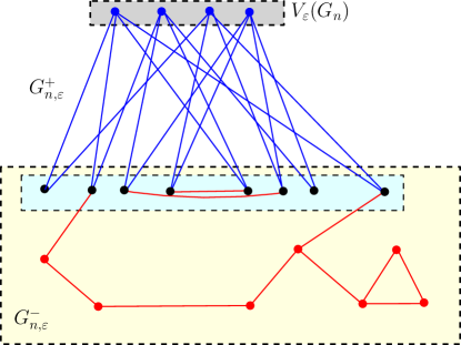
Figure 1. The decomposition of $G_{n,\varepsilon}$: The graph formed by the blue edges is $G_{n,\varepsilon}^{+}$ and the graph formed by the red edges is $G_{n,\varepsilon}^{-}$. Note that the black vertices belong to both $G_{n,\varepsilon}^{+}$ and $G_{n,\varepsilon}^{-}$.

The following lemma shows that the remainder term goes to zero in expectation, and therefore, in probability.

Lemma 2.3.

Let $R(K_{1,r},G_{n,\varepsilon})$ be as defined above in (2.4). Under the assumptions of Theorem 1.2,

$$\lim_{\varepsilon\rightarrow 0}\lim_{n\rightarrow\infty}\mathbb{E}(R(K_{1,r},G_{n,\varepsilon}))=0.$$

Proof.

Note that for $v\notin V_{\varepsilon}(G_{n})$

$$\sum_{\bm{u}\in{V(G_{n})\choose r-1}}a_{v}(\bm{u},G_{n})\leq d_{v}^{r-1}\leq(\varepsilon c_{n})^{r-1}.$$

Moreover $\sum_{v\notin V_{\varepsilon}(G_{n})}a_{vu_{1}}(G_{n,\varepsilon})\leq d_{u_{1}}$. Then, using (2.4), for any $M>0$,

$$\mathbb{E}(R(K_{1,r},G_{n,\varepsilon}))\leq \frac{(\varepsilon c_{n})^{r-1}}{c_{n}^{r}}\sum_{u_{1}\in V_{\varepsilon}(G_{n})}d_{u_{1}}$$

$$= \frac{\varepsilon^{r-1}}{c_{n}}\left(\sum_{u:\varepsilon c_{n}\leq d_{u}<M\varepsilon c_{n}}d_{u}+\sum_{u:d_{u}\geq M\varepsilon c_{n}}d_{u}\right)$$

$$\leq \frac{1}{c_{n}^{r}}\sum_{u:\varepsilon c_{n}\leq d_{u}<M\varepsilon c_{n}}d_{u}^{r}+\frac{1}{M^{r-1}c_{n}^{r}}\sum_{u\in V(G_{n})}d_{u}^{r}.$$ (2.5)

Since $\limsup_{n\rightarrow\infty}\frac{1}{c_{n}^{r}}\sum_{u\in V(G_{n})}d_{u}^{r}<\infty$ (from Observation 2.1), the second term in the RHS of (2.1) converges to $0$ on letting $n\rightarrow\infty$ followed by $M\rightarrow\infty$.

Next, recall that $\eta=\eta(\varepsilon)$ is such that $\theta_{\eta+1}<\varepsilon<\theta_{\eta}$. Thus, for all $n$ large enough, $d_{\eta+1}<\varepsilon c_{n}<d_{\eta}$, and as $n\rightarrow\infty$, the first term in the RHS above becomes

$$\limsup_{n\rightarrow\infty}\sum_{u=1}^{\eta}\frac{d_{u}^{r}}{c_{n}^{r}}\bm{1}\{d_{u}<M\varepsilon c_{n}\}\leq\sum_{u=1}^{\eta}\theta_{u}^{r}\bm{1}\{\theta_{u}\leq M\varepsilon\}=\sum_{u=1}^{\infty}\theta_{u}^{r}\bm{1}\{\varepsilon\leq\theta_{u}\leq M\varepsilon\},$$

which converges to $0$ on letting $\varepsilon\rightarrow 0$, by using DCT along with the fact that $\sum_{u=1}^{\infty}\theta_{u}^{r}\leq\limsup_{n\rightarrow\infty}\frac{1}{c_{n}^{r}}\sum_{u\in V(G_{n})}d_{u}^{r}<\infty$ (by Fatou’s lemma). ∎

Combining Lemma 2.2 and Lemma 2.3 it follows that

$$T(K_{1,r},G_{n})= T(K_{1,r},G_{n,\varepsilon})+o_{P}(1)$$

$$= T_{+}(K_{1,r},G_{n,\varepsilon}^{+})+T(K_{1,r},G_{n,\varepsilon}^{-})+o_{P}(1).$$ (2.6)

Therefore, the limiting distribution of the $T(K_{1,r},G_{n})$ is the same as that of $T_{+}(K_{1,r},G_{n,\varepsilon}^{+})+T(K_{1,r},G_{n,\varepsilon}^{-})$.

2.2. Independence in Moments of the Contributions from $G_{n,\varepsilon}^{+}$ and $G_{n,\varepsilon}^{-}$

In this section we show that the number of monochromatic $K_{1,r}$ coming from $G_{n,\varepsilon}^{+}$ and $G_{n,\varepsilon}^{-}$ are asymptotically independent in moments. Without loss of generality, assume the vertices in $V(G_{n})$ are labelled $1,2,\ldots,|V(G_{n})|$ such that $d_{1}\geq d_{2}\geq\cdots\geq d_{|V(G_{n})|}$, and $\eta=\eta(\varepsilon)$ such that $\theta_{\eta+1}<\varepsilon<\theta_{\eta}$ (assuming $\eta_{0}=\lim_{\varepsilon\rightarrow 0}\eta(\varepsilon)\geq 1$). Then, by definition (2.3),

$$T_{+}(K_{1,r},G_{n,\varepsilon}^{+})=\sum_{v=1}^{\eta}{T_{G_{n,\varepsilon}^{+}}(v)\choose r},\quad\text{where }T_{G_{n,\varepsilon}^{+}}(v):=\sum_{u\in V(G_{n,\varepsilon})}a_{uv}(G_{n})1\{X_{u}=X_{v}\},$$ (2.7)

is the number of monochromatic $r$-stars in $G_{n,\varepsilon}$, with central vertex $v\in V_{\varepsilon}(G_{n})$.

Now, fix a finite positive integer $K\leq\eta_{0}$. Then, for $\varepsilon>0$ small enough, $\eta(\varepsilon)\geq K$, and so $\{T_{G_{n,\varepsilon}^{+}}(v):1\leq v\leq K\}$ are well defined. The following lemma shows that this collection and $T(K_{1,2},G_{n,\varepsilon}^{-})$ are asymptotically independent in the moments.

Lemma 2.4.

Assume (1.4) holds. Then for every finite $K\leq\eta_{0}$ and non-negative integers $s,t_{1},\cdots,t_{K}$,

$$\lim_{\varepsilon\rightarrow 0}\lim_{n\rightarrow\infty}\left|\mathbb{E}\left({T}(K_{1,2},G_{n,\varepsilon}^{-})^{s}\prod_{v=1}^{K}T_{G_{n,\varepsilon}^{+}}(v)^{t_{v}}\right)-\mathbb{E}{T}(K_{1,2},G_{n,\varepsilon}^{-})^{s}\left(\mathbb{E}\prod_{v=1}^{K}T_{G_{n,\varepsilon}^{+}}(v)^{t_{v}}\right)\right|=0.$$ (2.8)

Proof of Lemma 2.4

For any labeled subgraph $H$ of $G_{n}$, define

$$\beta(H):=\mathbb{E}\prod_{(u,v)\in E(H)}\bm{1}\{X_{u}=X_{v}\}=\left(\frac{1}{c_{n}}\right)^{|V(H)|-\nu(H)},$$ (2.9)

where $\nu(H)$ is the number of connected components of $H$. Note that the definition of $\beta(\cdot)$ is invariant to the labelling of $H$, and so, it extends to unlabelled graphs as well. Thus, without loss of generality, we will define $\beta(H)$ as in (2.9), for an unlabelled graph $H$ as well.

Let $H_{1}=(V(H_{1}),E(H_{1}))$ and $H_{2}=(V(H_{2}),E(H_{2}))$ be two (labelled) subgraphs of $G_{n}$, that is, $V(H_{1})$ and $V(H_{2})$ are subsets of $V(G_{n})$, which inherits the labelling induced by $V(G_{n})$, and $E(H_{1})$ and $E(H_{2})$ are subsets of $E(H)$. Let $H_{1}\bigcup H_{2}=(V(H_{1})\bigcup V(H_{2}),E(H_{1})\bigcup E(H_{2}))$.

Lemma 2.5.

For any two finite graphs $H_{1}$ and $H_{2}$, $\beta\left(H_{1}\bigcup H_{2}\right)\geq\beta(H_{1})\beta(H_{2})$, where $\beta(\cdot)$ is defined above in (2.9).

Proof.

Denote by $F=H_{1}\bigcup H_{2}$, and let $F_{1},F_{2},\ldots,F_{\nu(F)}$ be the connected components of $F$. Define

$$I_{1}=\{s\in[\nu(F)]:V(F_{s})\bigcap V(H_{1})\neq\varnothing\text{ and }V(F_{s})\bigcap V(H_{2})=\varnothing\},$$

$$I_{2}=\{s\in[\nu(F)]:V(F_{s})\bigcap V(H_{1})=\varnothing\text{ and }V(F_{s})\bigcap V(H_{2})\neq\varnothing\},$$

$$I_{12}=\{s\in[\nu(F)]:V(F_{s})\bigcap V(H_{1})\neq\varnothing\text{ and }V(F_{s})\bigcap V(H_{2})\neq\varnothing\}.$$ (2.10)

Fix $s\in I_{12}$, that is, $V(F_{s})\bigcap V(H_{1})\neq\varnothing$ and $V(F_{s})\bigcap V(H_{2})\neq\varnothing$. Then $F_{s}=F_{s}^{\prime}\bigcup F_{s}^{\prime\prime}$, where

$$F_{s}^{\prime}=(V(F_{s})\bigcap V(H_{1}),E(F_{s})\bigcap E(H_{1})),\quad\text{and}\quad F_{s}^{\prime\prime}=(V(F_{s})\bigcap V(H_{2}),E(F_{s})\bigcap E(H_{2})).$$

Let $F_{s1}^{\prime},F_{s2}^{\prime}\ldots F_{sa}^{\prime}$ be the connected components of $F_{s}^{\prime}$ and similarly, $F_{s1}^{\prime\prime},F_{s2}^{\prime\prime}\ldots F_{sb}^{\prime\prime}$ be the connected components of $F_{s}^{\prime\prime}$, where $a=\nu(F_{s}^{\prime})$ and $b=\nu(F_{s}^{\prime\prime})$. Construct a bipartite graph $B_{s}=(B_{s}^{\prime}\bigcup B_{s}^{\prime\prime},E(B_{s}))$, where $B_{s}^{\prime}=\{F_{s1}^{\prime},F_{s2}^{\prime},\ldots F_{sa}^{\prime}\}$ and $B_{s}^{\prime\prime}=\{F_{s1}^{\prime\prime},F_{s2}^{\prime\prime},\ldots F_{sb}^{\prime\prime}\}$ and there is any edge between $F_{sx}^{\prime}$ and $F_{sy}^{\prime\prime}$ if and only if $V(F_{sx}^{\prime})\bigcap V(F_{sy}^{\prime\prime})\neq\varnothing$, for $x\in[a]$ and $y\in[b]$. Note that $|V(F_{s}^{\prime})\bigcap V(F_{s}^{\prime\prime})|\geq|E(B_{s})|$, and since the graph $F_{s}$ is connected, the graph $B_{s}$ is also connected. Therefore,

$$|V(F_{s}^{\prime})\bigcap V(F_{s}^{\prime\prime})|\geq|E(B_{s})|\geq|V(B_{s})|-1=\nu(F_{s}^{\prime})+\nu(F_{s}^{\prime\prime})-1,$$

This implies,

$$|V(F_{s})|=|V(F_{s}^{\prime})|+|V(F_{s}^{\prime\prime})|-|V(F_{s}^{\prime})\bigcap V(F_{s}^{\prime\prime})|\leq|V(F_{s}^{\prime})|-\nu(F_{s}^{\prime})+|V(F_{s}^{\prime\prime})|-\nu(F_{s}^{\prime\prime})+1.$$

Then, recalling (2.2), it follows that

$$\beta(H)= \prod_{s\in I_{1}}\beta(F_{s})\prod_{s\in I_{2}}\beta(F_{s})\prod_{s\in I_{12}}\beta(F_{s})$$

$$= \prod_{s\in I_{12}}\left(\frac{1}{c_{n}}\right)^{|V(F_{s})|-1}\prod_{s\in I_{1}}\beta(F_{s})\prod_{s\in I_{2}}\beta(F_{s})$$

$$\geq \left(\prod_{s\in I_{12}}\left(\frac{1}{c_{n}}\right)^{|V(F_{s}^{\prime})|-\nu(F_{s}^{\prime})}\prod_{s\in I_{1}}\beta(F_{s})\right)\left(\prod_{s\in I_{12}}\left(\frac{1}{c_{n}}\right)^{|V(F_{s}^{\prime\prime})|-\nu(F_{s}^{\prime\prime})}\prod_{s\in I_{2}}\beta(F_{s})\right)$$

$$= \beta(H_{1})\beta(H_{2}),$$

completing the proof of the lemma. ∎

Now, recall the definitions of the graph $G_{n,\varepsilon}^{-}$ from Section 2.1, and note that

$$T(K_{1,r},G_{n,\varepsilon}^{-}) =\sum_{\bm{u}\in\mathscr{S}_{r}(G_{n,\varepsilon}^{-})}\bm{1}\{X_{=\bm{u}}\},$$ (2.11)

where

• $\mathscr{S}_{r}(G_{n,\varepsilon}^{-})$ is the collection of ordered $(r+1)$-tuples $\bm{u}=(u_{0},u_{1},\cdots,u_{r})$, such that $u_{0},u_{1},\ldots,u_{r}\in V(G_{n,\varepsilon}^{-})$ are distinct and $(u_{0},u_{i})\in E(G_{n,\varepsilon}^{-})$, for $i\in[1,r]$; and

• $\bm{1}\{X_{=\bm{u}}\}=\bm{1}\{X_{u_{0}}=X_{u_{1}}=\cdots=X_{u_{r}}\}$.

For any $u\in V(G_{n})$, let $N_{G^{+}_{n,\varepsilon}}(u)$ be the neighborhood of $u$ in $G^{+}_{n,\varepsilon}$. Index the vertices in $N_{G^{+}_{n,\varepsilon}}(u)$ as $\{b_{1}(v),b_{2}(v),\ldots b_{d_{v}^{+}}(v)\}$, where $d_{v}^{+}$ is the degree of the vertex $v$ in $G^{+}_{n,\varepsilon}$. Let

$$\Gamma=\prod_{v=1}^{K}N_{G^{+}_{n,\varepsilon}}(v)^{t_{v}}\times\mathscr{S}_{r}(G_{n,\varepsilon}^{-})^{s}$$

denote the collection of vertices $\{b_{j}(v),1\leq j\leq t_{v},1\leq v\leq K\}$ and $s$ ordered $(r+1)$-tuples

$$\bm{u}_{1}=(u_{10},u_{11},u_{12},\cdots,u_{1r}),\bm{u}_{2}=(u_{20},u_{21},u_{22},\cdots,u_{2r}),\ldots,\bm{u}_{s}=(u_{s0},u_{s1},\ldots u_{sr}),$$

such that $b_{j}(v)\in N_{G^{+}_{n,\varepsilon}}(v)$, for $j\in[t_{v}]$ and $v\in[1,K]$, and $\bm{u}_{a}\in\mathscr{S}_{r}(G_{n,\varepsilon}^{-})$, for $a\in[1,s]$.

Then expanding the product ${T}(K_{1,2},G_{n,\varepsilon}^{-})^{s}\prod_{v=1}^{K}T_{G_{n,\varepsilon}^{+}}(v)^{t_{v}}$ over the sum, the LHS of (2.15) can be bounded above by:

$$\sum_{\Gamma}\Bigg{|}\mathbb{E}\left(\prod_{v=1}^{K}\prod_{j=1}^{t_{v}}\bm{1}\{X_{v}=X_{b_{j}(v)}\}\mathbb{E}\prod_{a=1}^{s}\bm{1}\{X_{=\bm{u}_{a}}\}\right)-\prod_{v=1}^{K}\left(\mathbb{E}\prod_{j=1}^{t_{v}}\bm{1}\{X_{v}=X_{b_{j}(v)}\}\mathbb{E}\prod_{a=1}^{s}\bm{1}\{X_{=\bm{u}_{a}}\}\right)\Bigg{|}$$

$$=\sum_{\Gamma}\left|\beta\left(H_{1}\bigcup H_{2}\right)-\beta(H_{1})\beta(H_{2})\right|$$ (2.12)

where $\beta(\cdot)$ is defined in (2.9) and

• $H_{1}$ is the simple labelled subgraph of $G_{n,\varepsilon}^{+}$ obtained by the union of the edges $(v,b_{j}(v))$ for $j\in[1,t_{v}]$ and $v\in[1,K]$.

• $H_{2}$ is the simple labelled subgraph of $G_{n,\varepsilon}^{-}$ obtained by the union of the $r$-stars formed by the collection of $(r+1)$-tuples $\{\bm{u}_{1},\cdots,\bm{u}_{s}\}$. More formally, $H_{2}=(V(H_{2}),E(H_{2}))$, where

  $$V(H_{2})=\bigcup_{j=1}^{s}\bm{u}_{j}\quad\text{and}\quad E(H_{2})=\bigcup_{j=1}^{s}\left\{(u_{j0},u_{ja}):1\leq a\leq r\right\}.$$

Note that if $V(H_{1})\bigcap V(H_{2})=\varnothing$, then $\beta\left(H_{1}\bigcup H_{2}\right)=\beta(H_{1})\beta(H_{2})$, and so without loss of generality we may assume that the sum over $\Gamma$ includes only terms for which $H_{1}\bigcap H_{2}\neq\varnothing$.

Definition 2.2.

Let $\mathcal{H}_{m_{1},m_{2}}$ denote the set of all unlabelled graphs $H=(V(H),E(H))$ which can be formed by the union of $m_{1}$ edges and $m_{2}$ copies of $K_{1,r}$.

Now, recalling that $\beta\left(H_{1}\bigcup H_{2}\right)=\beta(H_{1})\beta(H_{2})$, if $V(H_{1})\bigcap V(H_{2})=\varnothing$, and $\beta\left(H_{1}\bigcup H_{2}\right)\geq\beta(H_{1})\beta(H_{2})$ otherwise, the RHS of (2.2) can be bounded as follows:

$$\sum_{\Gamma}\left|\beta\left(H_{1}\bigcup H_{2}\right)-\beta(H_{1})\beta(H_{2})\right| \leq\sum_{\Gamma}\beta\left(H_{1}\bigcup H_{2}\right)$$

$$=\sum_{m_{1}=1}^{s_{1}}\sum_{m_{2}=1}^{s_{2}}\sum_{H\in\mathcal{H}_{m_{1},m_{2}}}\sum_{\Gamma:H_{1}\bigcup H_{2}\cong H}\beta\left(H_{1}\bigcup H_{2}\right)$$

$$\lesssim\sum_{m_{1}=1}^{s_{1}}\sum_{m_{2}=1}^{s_{2}}\sum_{H\in\mathcal{H}_{m_{1},m_{2}}}\beta(H)N(H,G_{n,\varepsilon}^{+}[K],G_{n,\varepsilon}^{-}),$$ (2.13)

where

• $G_{n,\varepsilon}^{+}[K]$ be the induced sub-graph of $G_{n,\varepsilon}^{+}$ formed by the vertices labeled $\{1,2,\ldots,K\}$, that is, the $K$ highest degree vertices in $G_{n}$; and

• $N(H,G_{n,\varepsilon}^{+}[K],G_{n,\varepsilon}^{-})$ is the number of copies of $H=H_{1}\bigcup H_{2}$ in $G_{n,\varepsilon}^{+}[K]\bigcup G_{n,\varepsilon}^{-}$, such that $H_{1}$ is formed by the union of $m_{1}$ edges from $G_{n,\varepsilon}^{+}[K]$ and $H_{2}$ is formed by the union of $m_{2}$ copies of $K_{1,r}$ from $G_{n,\varepsilon}^{-}$, and $V(H_{1})\bigcap V(H_{2})\neq\varnothing$.

Now, using $\beta(H)=\frac{1}{c_{n}^{|V(H)|-\nu(H)}}$ (by Lemma 2.5), and since the sum over $m_{1},m_{2},H$ in (2.2) are all finite, to prove (2.15) it suffices to show that for every $H\in\mathcal{H}_{m_{1},m_{2}}$,

$$\limsup_{\varepsilon\rightarrow 0}\limsup_{n\rightarrow\infty}\frac{N(H,G_{n,\varepsilon}^{+}[K],G_{n,\varepsilon}^{-})}{c_{n}^{V(H)-\nu(H)}}=0.$$ (2.14)

To this end, fix $H\in\mathcal{H}_{m_{1},m_{2}}$ such that $H=H_{1}\bigcup H_{2}$, such that $H_{1}$ is formed by the union of $m_{1}$ edges from $G_{n,\varepsilon}^{+}[K]$ and $H_{2}$ is formed by the union of $m_{2}$ copies of $K_{1,r}$ from $G_{n,\varepsilon}^{-}$, and $V(H_{1})\bigcap V(H_{2})\neq\varnothing$ (otherwise $N(H,G_{n,\varepsilon}^{+}[K],G_{n,\varepsilon}^{-})=0$). Let $C_{1},C_{2},\ldots,C_{\nu(H)}$ the connected components of $H$. Fix $1\leq j\leq\nu(H)$ and consider the following three cases:

• $V(C_{j})$ only intersects $V(H_{1})$. Since $G_{n,\varepsilon}^{+}[K]$ is a bi-partite graph with bi-partition with $|E(G_{n,\varepsilon}^{+}[K])|\leq K\Delta(G_{n})\lesssim_{r}Kc_{n}$ (using $\Delta(G_{n})=O(c_{n})$). This gives

  $$N(C_{j},G_{n,\varepsilon}^{+}[K])\leq|E(G_{n,\varepsilon}^{+}[K])|^{|V(C_{j})|-1}\lesssim_{r,m_{1}}(Kc_{n})^{|V(C_{j})|-1}.$$

• $V(C_{j})$ only intersects $V(H_{2})$. Then there exists $1\leq h\leq m_{2}$ such that $H_{2}$ is spanned by $h$ isomorphic copies of $K_{1,r}$. Thus, using the bounds $N(K_{1,r},G_{n})=\Theta(c_{n}^{r})$ and gives the bound

  $$N(C_{j},G_{n,\varepsilon}^{-})\leq N(K_{1,r},G_{n})\Delta(G_{n})^{|V(C_{j})|-r+1}\lesssim_{r,m_{2}}c_{n}^{|V(C_{j})|-1},$$

  using $\Delta(G_{n})=O(c_{n})$.

• $V(C_{j})$ intersects both $V(H_{1})$ and $V(H_{2})$. If $C_{j}$ is such that it intersects both $H_{1}$ and $H_{2}$, then there is a vertex $v\in V(H_{1})\bigcap V(H_{2})$, such that $(u,v)$ is an edge in $G_{n,\varepsilon}^{+}[K]$, and $(v,w)$ is an edge $G_{n,\varepsilon}^{-}$. Thus, using the estimate $\Delta(G_{n})=O(c_{n})$,

  $$N(C_{j},G_{n,\varepsilon}^{+}[K],G_{n,\varepsilon}^{-}) \lesssim|E(G_{n,\varepsilon}^{+}[K])|\left(\max_{v\in V(G_{n,\varepsilon}^{-})}d_{v}\right)\Delta(G_{n})^{|V(C_{j})|-3}$$

  $$\lesssim_{r,m_{1},m_{2}}K\varepsilon c_{n}^{|V(C_{j})|-1}.$$

Taking a product over $1\leq j\leq\nu(H)$ and, since $V(H_{1})\bigcap V(H_{2})\neq\varnothing$, gives

$$N(H,G_{n,\varepsilon}^{+}[K],G_{n,\varepsilon}^{-})\lesssim_{r,m_{1},m_{2}} \varepsilon K^{|V(H)|-\nu(H)}c_{n}^{|V(H)|-\nu(H)},$$

which implies (2.14), from which the desired conclusion follows. ∎

2.3. Contribution from $G_{n,\varepsilon}^{+}$

In this section we compute the asymptotic distribution of $T_{+}(K_{1,r},G_{n,\varepsilon}^{+})$ (recall (2.3)). This involves showing that the collection $\{T_{G_{n,\varepsilon}^{+}}(v):1\leq v\leq K\}$ are asymptotically independent, by another moment comparison.

Lemma 2.6.

Assume (1.4) holds, and $\varepsilon>0$ small enough. Then for all non-negative integers $s_{1},\cdots,s_{K}$,

$$\lim_{n\rightarrow\infty}\left|\mathbb{E}\left(\prod_{v=1}^{K}T_{G_{n,\varepsilon}^{+}}(v)^{s_{v}}\right)-\prod_{v=1}^{K}\mathbb{E}T_{G_{n,\varepsilon}^{+}}(v)^{s_{v}}\right|=0.$$ (2.15)

As a consequence, $T_{+}(K_{1,r},G_{n,\varepsilon}^{+})\stackrel{{\scriptstyle D}}{{\to}}\sum_{v=1}^{\eta}{T_{v}\choose r}$, as $n\rightarrow\infty$, where $T_{1},T_{2},\ldots,T_{\eta}$ are independent $\operatorname{Pois}(\theta_{1}),\operatorname{Pois}(\theta_{2}),\ldots,\operatorname{Pois}(\theta_{\eta})$, respectively. $($Recall that $\eta=\eta(\varepsilon)$ is such that $\theta_{\eta+1}<\varepsilon<\theta_{\eta}$.$)$

Proof.

Expanding the moments, we have

$$\left|\mathbb{E}\prod_{v=1}^{K}T_{G_{n,\varepsilon}^{+}}(v)^{s_{v}}-\prod_{v=1}^{K}\mathbb{E}T_{G_{n,\varepsilon}^{+}}(v)^{s_{v}}\right| =\sum_{\Gamma}\left|\mathbb{E}\prod_{v=1}^{K}\prod_{j=1}^{s_{v}}\bm{1}\{X_{v}=X_{b_{j}(v)}\}-\prod_{v=1}^{K}\mathbb{E}\prod_{j=1}^{s_{v}}\bm{1}\{X_{v}=X_{b_{j}(v)}\}\right|$$

$$=\sum_{\Gamma}\left|\beta\left(\bigcup_{v=1}^{K}H(v)\right)-\prod_{v=1}^{K}\beta(H(v))\right|$$

where

• $\Gamma$ is the collection of all possible choices of $b_{j}(v)\in N_{G_{n,\varepsilon}}(v)$, for $j\in[s_{v}]$ and $v\in[K]$; and

• $H(v)$ denotes the simple graph formed by union of all the edges $(v,b_{j}(v))$, for $j\in[s_{v}]$. Note that $H(v)$ is isomorphic to a star graph, for every $v\in[K]$.

If $\bigcup_{v=1}^{K}H(v)$ is a forest, then the collection of random variables $\{\bm{1}\{X_{v}=X_{b_{j}(v)},j\in[s_{v}],v\in[K]\}$ are mutually independent, and so, $\beta(\bigcup_{v=1}^{K}H(v))=\prod_{v=1}^{K}\beta(H(v))$. Thus, without loss of generality, assume that $\bigcup_{v=1}^{K}H(v)$ is not a forest, that is, it contains a cycle. Then denoting $\mathcal{H}_{m}$ to be the set of unlabelled graphs with $m$ vertices and $s:=\sum_{v=1}^{K}s_{v}$, using Lemma 2.5 gives

$$\left|\mathbb{E}\prod_{v=1}^{K}T_{G_{n,\varepsilon}^{+}}(v)^{s_{v}}-\prod_{v=1}^{K}\mathbb{E}T_{G_{n,\varepsilon}^{+}}(v)^{s_{v}}\right|\lesssim \sum_{m=2}^{2s}\sum_{\begin{subarray}{c}H\in\mathcal{H}_{m}\\ H\text{ contains a cycle }\end{subarray}}\sum_{\Gamma:\bigcup_{v=1}^{K}H(v)\simeq H}\beta\left(\bigcup_{v=1}^{K}H(v)\right)$$

$$= \sum_{m=2}^{2s}\sum_{\begin{subarray}{c}H\in\mathcal{H}_{m}\\ H\text{ contains a cycle }\end{subarray}}N(H,G_{n,\varepsilon}^{+}[K])\beta(H)$$

$$= \sum_{m=2}^{2s}\sum_{\begin{subarray}{c}H\in\mathcal{H}_{m}\\ H\text{ contains a cycle }\end{subarray}}\frac{N(H,G_{n,\varepsilon}^{+}[K])}{c_{n}^{|V(H)|-\nu(H)}}.$$ (2.16)

Now, fix $H\in\mathcal{H}_{m}$ with connected components $H_{1},H_{2},\ldots,H_{\nu(H)}$, and assume without loss of generality that $H_{1}$ contains a cycle of length $g\geq 3$. Invoking [3, Lemma 2.3] gives,

$$N(H_{1},G_{n,\varepsilon}^{+}[K])\lesssim|E(G_{n,\varepsilon}^{+}[K])|^{|V(H_{1})|-g/2}\lesssim(K\Delta(G_{n}))^{|V(H_{1})|-g/2},$$

where the last inequality uses $|E(G_{n,\varepsilon}^{+}[K]|\leq K\Delta(G_{n})$. Also, by [3, Lemma 2.3], for $j\geq 2$,

$$N(H_{j},G_{n,\varepsilon}^{+}[K])\lesssim|E(G_{n,\varepsilon}^{+}[K])|^{|V(H_{j})|-1}\leq(K\Delta(G_{n}))^{|V(H_{j})|-1}.$$

Taking a product over $j$ and using $\Delta(G_{n})=O(c_{n})$, gives

$$N(H,G_{n,\varepsilon}^{+}[K])\leq\prod_{j=1}^{\nu(H)}N(H_{j},G_{n})\lesssim K^{|V(H)|-\nu(H)|}c_{n}^{|V(H)|-g/2},$$

which implies $\limsup_{n\rightarrow\infty}\frac{N(H,G_{n,\varepsilon}^{+}[K])}{c_{n}^{|V(H)|-\nu(H)}}=0$, as $g\geq 3$. Since the sum in (2.3) is finite (does not depend on $n,\varepsilon$), the conclusion in (2.15) follows.

Moreover, since $T_{G_{n,\varepsilon}^{+}}(v)\rightarrow\operatorname{Pois}(\theta_{v})$ in distribution and in moments, (2.15) implies that

$$\lim_{n\rightarrow\infty}\left|\mathbb{E}\left(\prod_{v=1}^{\eta}T_{G_{n,\varepsilon}^{+}}(v)^{s_{v}}\right)-\prod_{v=1}^{\eta}\mathbb{E}\operatorname{Pois}(\theta_{v})^{s_{v}}\right|.$$

This implies, as the Poisson distribution is uniquely determined by its moments,

$$(T_{G_{n,\varepsilon}^{+}}(1),T_{G_{n,\varepsilon}^{+}}(2),\ldots,T_{G_{n,\varepsilon}^{+}}(\eta))\rightarrow(T_{1},T_{2},\ldots,T_{\eta}),$$

as $n\rightarrow\infty$, in distribution and in moments, where $T_{1},T_{2},\ldots,T_{\eta}$ are independent $\operatorname{Pois}(\theta_{1}),\operatorname{Pois}(\theta_{2})$, $\ldots,\operatorname{Pois}(\theta_{\eta})$, respectively. Finally, recalling (2.7) and by the continuous mapping theorem $T_{+}(K_{1,r},G_{n,\varepsilon}^{+})=\sum_{v=1}^{\eta}{T_{G_{n,\varepsilon}^{+}}(v)\choose r}\rightarrow\sum_{v=1}^{\eta}{T_{v}\choose r}$ in distribution and in moments, as $n\rightarrow\infty$. ∎

2.4. Contribution from $G_{n,\varepsilon}^{-}$

In this section we derive the limiting distribution of $T(K_{1,r},G_{n,\varepsilon}^{-})$, by invoking [4, Theorem 2.1], which gives conditions under which the number of monochromatic subgraphs (in particular monochromatic stars) converges to a linear combination of Poisson variables.

Lemma 2.7.

As $n\rightarrow\infty$ followed by $\varepsilon\rightarrow 0$,

$$T(K_{1,r},G_{n,\varepsilon}^{-})\rightarrow\sum_{k=1}^{r+1}kZ_{k},$$

in distribution and in moments, where $Z_{1},Z_{2},\ldots,Z_{r+1}$ are independent $\operatorname{Pois}(\lambda_{1}-\frac{1}{r!}\sum_{u=1}^{\infty}\theta_{u}^{r})$, $\operatorname{Pois}(\lambda_{2}),\ldots\operatorname{Pois}(\lambda_{r+1})$, respectively.

Proof of Lemma 2.7

We will prove this result by invoking [4, Theorem 2.1]. To begin with, let $F$ be a graph formed by union of two isomorphic copies of $K_{1,r}$, such that $|V(F)|>r+1$. Then $F$ is connected, and

$$N(F,G_{n,\varepsilon}^{-})\lesssim N(K_{1,r},G_{n,\varepsilon}^{-})\cdot\Delta(G_{n})^{|V(F)|-r-1} \leq N(K_{1,r},G_{n})\cdot(\varepsilon c_{n})^{|V(F)|-r-1}$$

$$=\varepsilon^{|V(F)|-r-1}c_{n}^{|V(F)|-1}.$$

Therefore, $\frac{1}{c_{n}^{|V(F)|-1}}N(F,G_{n,\varepsilon}^{-})=o(1)$, $n\rightarrow\infty$ followed by $\varepsilon\rightarrow 0$, when $|V(F)|>r+1$.

It remains to consider super-graphs $F\supseteq K_{1,r}$ with $|V(F)|=r+1$. Recalling $\mathscr{C}_{r,k}:=\{F\supseteq K_{1,r}:|V(F)|=r+1\text{ and }N(K_{1,r},F)=k\}$, we have the following lemma.

Lemma 2.8.

For any $F\in\mathscr{C}_{r,k}$, with $k\in[2,r+1]$, $N_{\mathrm{ind}}(F,G_{n,\varepsilon})=N_{\mathrm{ind}}(F,G_{n,\varepsilon}^{-})+o(c_{n}^{r})$, as $n\rightarrow\infty$ followed by $\varepsilon\rightarrow 0$.

Proof.

Let $k\in[2,r+1]$ and suppose $F\in\mathscr{C}_{r,k}$ is an induced subgraph of $G_{n,\varepsilon}$, such that $V(F)$ is not completely contained in $V(G_{n,\varepsilon}^{-})$. Then, since $F$ has at least two vertices of degree $r$ and any two degree $r$ vertices must be neighbors, the vertices of $F$ can be spanned by a $r$-star whose central vertex is in $N_{G_{n,\varepsilon}}(V_{\varepsilon}(G_{n}))$. Therefore, the difference $N_{\mathrm{ind}}(F,G_{n,\varepsilon})-N_{\mathrm{ind}}(F,G_{n,\varepsilon}^{-})$ is bounded above by (up to constants depending only on $r$)

$$\sum_{v\notin V_{\varepsilon}(G_{n})}\sum_{u_{1}\in V_{\varepsilon}(G_{n})}\sum_{\bm{u}\in{V(G_{n})\choose r-1}}a_{vu_{1}}(G_{n})a_{v}(\bm{u},G_{n}),$$ (2.17)

which is $o(c_{n}^{r})$ (from the proof of Lemma 2.3). ∎

Using the above lemma and $N_{\mathrm{ind}}(F,G_{n})=N_{\mathrm{ind}}(F,G_{n,\varepsilon})+o(c_{n}^{r})$ (by Lemma 2.2), it follows that, for $k\in[2,r+1]$,

$$\lim_{\varepsilon\rightarrow 0}\lim_{n\rightarrow\infty}\frac{\sum_{F\in\mathscr{C}_{r,k}}N_{\mathrm{ind}}(F,G_{n,\varepsilon}^{-})}{c_{n}^{r}}=\lim_{\varepsilon\rightarrow 0}\lim_{n\rightarrow\infty}\frac{\sum_{F\in\mathscr{C}_{r,k}}N_{\mathrm{ind}}(F,G_{n})}{c_{n}^{r}}=\lambda_{k},$$

where the last equality uses (1.5).

It remains to consider the case $k=1$. To begin with, observe that for any graph $G$,

$$N(K_{1,r},G)=\sum_{k=1}^{r+1}\sum_{F\in\mathscr{C}_{r,k}}kN_{\mathrm{ind}}(F,G).$$ (2.18)

Moreover, using Lemma 2.2 and (2.1) gives

$$N(K_{1,r},G_{n,\varepsilon}^{-}) =N(K_{1,r},G_{n})-\sum_{v=1}^{\eta}{d_{v}\choose r}+o(c_{n}^{r}).$$

Now, using this and (2.18) with $G=G_{n,\varepsilon}^{-}$ gives

$$\frac{\sum_{F\in\mathscr{C}_{r,1}}N_{\mathrm{ind}}(F,G_{n,\varepsilon}^{-})}{c_{n}^{r}} =\frac{N(K_{1,r},G_{n})}{c_{n}^{r}}-\frac{1}{c_{n}^{r}}\sum_{v=1}^{\eta}{d_{v}\choose r}-\sum_{k=2}^{r+1}k\sum_{F\in\mathscr{C}_{r,k}}\frac{N_{\mathrm{ind}}(F,G_{n,\varepsilon}^{-})}{c_{n}^{r}}+o(1)$$

$$\rightarrow\sum_{k=1}^{r+1}k\lambda_{k}-\sum_{u=1}^{\infty}\frac{\theta_{u}^{r}}{r!}-\sum_{k=2}^{r+1}k\lambda_{k} G=G_{n}$$ (using (2.18) with and (1.5))

$$=\lambda_{1}-\sum_{u=1}^{\infty}\frac{\theta_{u}^{r}}{r!},$$

as $n\rightarrow\infty$ followed by $\varepsilon\rightarrow 0$. Then by [4, Theorem 2.1], we have $T(K_{1,r},G_{n,\varepsilon}^{-})\stackrel{{\scriptstyle D}}{{\to}}\sum_{k=1}^{r+1}kZ_{k}$, where $Z_{1},Z_{2},\ldots,Z_{r+1}$ are as in the statement of the lemma.

The convergence in moments is a consequence of uniform integrability as $\mathbb{E}(T(K_{1,r},G_{n,\varepsilon}^{-}))\leq\mathbb{E}T(K_{1,r},G_{n})^{r}=O_{r}(1)$ for every fixed integer $r\geq 1$ [3, Theorem 1.2].

2.5. Completing the Proof of Theorem 1.2

To begin use Lemma 2.3 to note that it suffices to find the limiting distribution of

$$\sum_{v=1}^{\eta}{T_{G_{n,\varepsilon}^{+}}(v)\choose r}+T(K_{1,r},G_{n,\varepsilon}^{-}),$$

under the double limit as $n\rightarrow\infty$ followed by $\varepsilon\rightarrow 0$. Fix an integer $M\geq 1$ and write the above random variable as

$$\sum_{v=1}^{M}{T_{G_{n,\varepsilon}^{+}}(v)\choose r}+\sum_{v=M+1}^{\eta}{T_{G_{n,\varepsilon}^{+}}(v)\choose r}+T(K_{1,r},G_{n,\varepsilon}^{-}).$$

Under the double limit the random vector

$$\Big{(}T_{G_{n,\varepsilon}^{+}}(1),\cdots,T_{G_{n,\varepsilon}^{+}}(M),T(K_{1,r},G_{n,\varepsilon}^{-})\Big{)}\stackrel{{\scriptstyle D}}{{\to}}\left(T_{1},\cdots,T_{M},\sum_{k=1}^{r+1}kZ_{k}\right),$$

by invoking Lemmas 2.4, 2.6 and 2.7. By continuous mapping theorem this gives

$$\sum_{v=1}^{M}{T_{G_{n,\varepsilon}^{+}}(v)\choose r}+T(K_{1,r},G_{n,\varepsilon}^{-})\stackrel{{\scriptstyle D}}{{\rightarrow}}\sum_{v=1}^{M}{T_{v}\choose r}+\sum_{k=1}^{r+1}kZ_{k},$$

the RHS of which on letting $p\rightarrow\infty$ converges in distribution to $\sum_{v=1}^{\infty}{T_{v}\choose r}+\sum_{k=1}^{r+1}kZ_{k}$. It thus suffices to show that

$$\lim_{M\rightarrow\infty}\lim_{\varepsilon\rightarrow 0}\lim_{n\rightarrow\infty}\sum_{v=M+1}^{\eta}\mathbb{E}{T_{G_{n,\varepsilon}^{+}}(v)\choose r}=0.$$

The LHS above is bounded above by $\sum_{v=M+1}^{\eta}\frac{1}{r!}\frac{d_{v}^{r}}{c_{n}^{r}}$, which on letting $n\rightarrow\infty$ followed by $\varepsilon\rightarrow 0$ gives $\frac{1}{r!}\sum_{v=M+1}^{\infty}\theta_{v}^{r}$. This converges to $0$ as $M\rightarrow\infty$, as $\sum_{v=1}^{\infty}\theta_{v}^{r}<\infty$, as noted in the proof of Lemma 2.3. (Note that if $\lim_{\varepsilon\rightarrow 0}\eta(\varepsilon):=L<\infty$, then the term $\sum_{v=L+1}^{\eta}{T_{G_{n,\varepsilon}^{+}}(v)\choose r}+T(K_{1,r},G_{n,\varepsilon}^{-})$ vanishes, thus simplifying the proof. )

Finally, the convergence in moments is a consequence of uniform integrability as all moments of $T(K_{1,r},G_{n})$ are bounded: that is, $\mathbb{E}T(K_{1,r},G_{n})^{r}=O_{r}(1)$ for every fixed integer $r\geq 1$ (this follows from the proof of [3, Theorem 1.2]).

To prove the converse, invoking Proposition 1.1 we can assume, without loss of generality, that $N(K_{1,r},G_{n})=O(c_{n}^{r})$. This in turn implies that for every graph $F$ on $r+1$ vertices which is a super graph of $K_{1,r}$ we have $N_{\text{ind}}(F,G_{n})=O(c_{n}^{r})$. Thus by passing to a subsequence, assume that $N_{\text{ind}}(F,G_{n})/c_{n}^{r}$ converges for every $F$ which is a super graph of $K_{1,r}$. This implies existence of the limits in (1.5). Finally, using (2.2) we have $\max_{v\in V(G_{n})}d_{v}=O(c_{n})$, and so the infinite tuple $\{d_{v}/c_{n}\}_{v\geq 1}$ is an element of $[0,K]^{\mathbb{N}}$ for some $K$ fixed. Since $[0,K]^{\mathbb{N}}$ is compact in product topology, there is a further subsequence along which $d_{v}/c_{n}$ converges for every $v\geq 1$ simultaneously. Thus, moving to a subsequence, we can assume that $d_{v}/c_{n}$ converges to $\theta_{v}$ for every $v$. Invoking the sufficiency part of the theorem gives that $T(K_{1,r},G_{n})$ converges in distribution to a random variable of the desired form, completing the proof.

2.6. Proof of Corollary 1.3

The proof of $(a)\Rightarrow(b)$ is immediate from Theorem 1.2, so it suffices to prove $(b)\Rightarrow(a)$. To this end, note that $T(K_{1,r},G_{n})\stackrel{{\scriptstyle D}}{{\to}}\sum_{k=1}^{r+1}kZ_{k}$ implies that (1.4) holds (Proposition 1.1). Thus, by a similar argument which was used to prove the converse of Theorem 1.2, it follows that along a subsequence the limits $\lim_{n\rightarrow\infty}\frac{1}{c_{n}^{r}}N_{\text{ind}}(F,G_{n})$ exist for all super graphs $F$ of $K_{1,r}$ on $r+1$ vertices, and so, for $k\in[1,r+1]$,

$$\lambda^{\prime}_{k}:=\lim_{n\rightarrow\infty}\sum_{F\in\mathcal{C}_{r,k}}\frac{N_{\text{ind}}(F,G_{n})}{c_{n}^{r}}$$

is well defined. Then, as before, by passing to another subsequence the limits $\theta^{\prime}_{v}:=\lim_{n\rightarrow\infty}\frac{d_{v}}{c_{n}}$ exist for every $v\geq 1$, and by the if part of Theorem 1.2 along this subsequence,

$$T(K_{1,r},G_{n})\stackrel{{\scriptstyle d}}{{\rightarrow}}\sum_{v=1}^{\infty}{T_{v}^{\prime}\choose r}+\sum_{k=1}^{r+1}kZ_{k}^{\prime},$$

where $\{T_{v}^{\prime}\}_{v\geq 1}$ and $\{Z_{k}^{\prime}\}_{1\leq k\leq r+1}$ are mutually independent, and $T_{1}^{\prime},T_{2}^{\prime},\ldots,$ are independent $\operatorname{Pois}(\theta_{1}^{\prime})$, $\operatorname{Pois}(\theta_{2}^{\prime}),\ldots$, respectively, and $Z_{1}^{\prime},Z_{2}^{\prime},\ldots,Z_{r+1}^{\prime}$ are independent $\operatorname{Pois}(\lambda_{1}^{\prime}-\frac{1}{r!}\sum_{u=1}^{\infty}(\theta_{u}^{\prime})^{r}),\operatorname{Pois}(\lambda_{2}^{\prime})$, $\ldots,\operatorname{Pois}(\lambda_{r+1}^{\prime})$, respectively.

However, since $T(K_{1,r},G_{n})$ converges in distribution to $\sum_{k=1}^{r+1}kZ_{k}$ which has finite exponential moment everywhere, it follows that $\theta_{v}^{\prime}=0$ for all $v\geq 1$, and consequently, the maximum degree $\Delta(G_{n})=o(c_{n})$. This also gives

$$\sum_{k=1}^{r+1}kZ_{k}\stackrel{{\scriptstyle D}}{{=}}\sum_{k=1}^{r+1}kZ^{\prime}_{k},$$

and so the corresponding probability generating functions must match, that is,

$$\prod_{k=1}^{r+1}e^{\lambda_{k}(s^{k}-1)}=\prod_{k=1}^{r+1}e^{\lambda_{k}^{\prime}(s^{k}-1)},\quad\text{for all }s\in(0,1).$$

This implies, $\sum_{k=1}^{r+1}\lambda_{k}(s^{k}-1)=\sum_{k=1}^{r+1}\lambda_{k}^{\prime}(s^{k}-1)$, for all $s\in(0,1)$, and so the corresponding coefficients must be equal, giving $\lambda_{k}=\lambda_{k}^{\prime}$. Therefore, every sub sequential limit of $\sum_{F\in\mathcal{C}_{r,k}}\frac{N_{\text{ind}}(K_{1,r},G_{n})}{c_{n}^{r}}$ equal $\lambda_{k}$, for $k\in[1,r+1]$, hence, (1.5) holds.

3. Examples

In this section we apply Theorem 1.2 to different deterministic and random graph models, and determine the specific nature of the limiting distribution.

Example 1.

(Disjoint Union of Stars) The proof of Theorem 1.2 shows that the quadratic term in the limiting distribution of $T(K_{1,r},G_{n})$ appears due to the $r$-stars incident on vertices with degree $\Theta(c_{n})$. This can be seen when $G_{n}$ is a disjoint union of star graphs.

• To begin with suppose $G_{n}=K_{1,n}$ is the $n$-star. Then $N(K_{1,r},K_{1,n})={n\choose r}$, and if we color $K_{1,n}$ with $c_{n}$ colors such that $n/c_{n}\rightarrow 1$, then $\mathbb{E}(T(K_{1,r},G_{n}))=\frac{1}{r!}$. Note that the maximum degree $d_{(1)}=n$, which implies $\theta_{1}=1$. Moreover, $d_{(2)}=1$, which implies $\theta_{v}=0$, for all $v\geq 2$. Therefore, by Theorem 1.2,

  $$T(K_{1,r},G_{n})\stackrel{{\scriptstyle D}}{{\to}}{T_{1}\choose r},$$

  where $T_{1}\sim\operatorname{Pois}(1)$. (Note that the graph $G_{n,\varepsilon}^{-}$ is empty in this case.)

• Next, consider $G_{n}$ to be the disjoint union of the following stars: $K_{1,\lfloor na_{1}\rfloor},K_{1,\lfloor na_{2}\rfloor},\ldots,K_{1,\lfloor na_{n}\rfloor}$, such that $\sum_{s=1}^{\infty}a_{s}^{r}<\infty$. In this case, $N(K_{1,r},G_{n})=\sum_{s=1}^{n}{\lfloor na_{s}\rfloor\choose r}\sim\frac{n^{r}}{r!}\sum_{s=1}^{n}a_{s}^{r}$. If $G_{n}$ is colored with $c_{n}$ colors such that $n/c_{n}\rightarrow 1$, then $\mathbb{E}(T(K_{1,r},G_{n}))\rightarrow\frac{1}{r!}\sum_{s=1}^{\infty}a_{s}^{r}$. Also, $d_{(v)}=\lfloor na_{v}\rfloor$, which implies $\theta_{v}=a_{v},$ for $v\geq 1$. This implies, by Theorem 1.2,

  $$T(K_{1,r},G_{n})\stackrel{{\scriptstyle D}}{{\to}}\sum_{s=1}^{\infty}{T_{s}\choose r},$$

  where $T_{s}\sim\operatorname{Pois}(a_{s})$ and $T_{1},T_{2},\ldots$ are independent. Here, the linear terms linear in Poisson do not contribute, as $G_{n,\varepsilon}^{-}$ is empty, and $\mathbb{E}T(K_{1,r},G_{n})\sim\frac{1}{r!}\sum_{v=1}^{\infty}\theta_{v}^{r}$.

• Finally, consider $G_{n}$ to be the disjoint union of the following stars:

  $$K_{1,\lfloor na_{1}+n^{\frac{r-1}{r}}\rfloor},K_{1,\lfloor na_{2}+n^{\frac{r-1}{r}}\rfloor},\ldots,K_{1,\lfloor na_{n}+n^{\frac{r-1}{r}}\rfloor}.$$

  In this case,

  $$N(K_{1,r},G_{n})=\sum_{s=1}^{n}{\lfloor na_{s}+n^{\frac{r-1}{r}}\rfloor\choose r}\sim\frac{n^{r}}{r!}+\frac{n^{r}}{r!}\sum_{s=1}^{n}a_{s}^{r},$$

  since $\sum_{s=1}^{n}a_{s}^{k}=o(n^{1-\frac{k}{r}})$, for $1\leq k<r$ (see Observation 3.1 below). If $G_{n}$ is colored with $c_{n}$ colors such that $n/c_{n}\rightarrow 1$, then $\mathbb{E}(T(K_{1,r},G_{n}))\rightarrow\frac{1}{r!}\left(1+\sum_{s=1}^{\infty}a_{s}^{r}\right)$. Also, $d_{(v)}=\lfloor na_{v}+n^{\frac{r-1}{r}}\rfloor$, which implies $\theta_{v}=a_{v},$ for $v\geq 1$, and so Theorem 1.2 gives

  $$T(K_{1,r},G_{n})\stackrel{{\scriptstyle D}}{{\to}}\sum_{s=1}^{\infty}{T_{s}\choose r}+Z,$$

  where $T_{s}\sim\operatorname{Pois}(a_{s})$ and $T_{1},T_{2},\ldots$ are independent, and $Z\sim\operatorname{Pois}(\frac{1}{r!})$ independent of $\{T_{s}\}_{s\geq 1}$.

Observation 3.1.

If $\{a_{s}\}_{s\geq 1}$ is a sequence of non-negative real numbers such that $\sum_{s=1}^{\infty}a_{s}^{r}<\infty$ then $\sum_{s=1}^{n}a_{s}^{k}=o(n^{1-\frac{k}{r}})$, for $1\leq k<r$.

Proof.

Fixing $\varepsilon>0$ and a positive integer $N\geq 1$ we get

$$\sum_{s=1}^{n}a_{s}^{k}= \sum_{s=1}^{N}a_{s}^{k}+\sum_{s=N+1}^{n}a_{s}^{k}\bm{1}\{a_{s}\leq\varepsilon n^{-\frac{1}{r}}\}+\sum_{s=N+1}^{n}a_{s}^{k}\bm{1}\{a_{s}>\varepsilon n^{-\frac{1}{r}}\}$$

$$\leq \sum_{s=1}^{N}a_{s}^{k}+\varepsilon^{k}n^{1-\frac{k}{r}}+\frac{n^{1-\frac{r}{k}}}{\varepsilon^{r-k}}\sum_{s=N+1}^{\infty}a_{s}^{r}.$$

On dividing by $n^{1-\frac{k}{r}}$ and letting $n\rightarrow\infty$, the first term goes to $0$ as it is a finite sum, and, therefore,

$$\limsup_{n\rightarrow\infty}\frac{\sum_{s=1}^{k}a_{s}^{r}}{n^{1-\frac{k}{r}}}\leq\varepsilon^{k}+\frac{1}{\varepsilon^{r-k}}\sum_{s=N+1}^{\infty}a_{s}^{r}.$$

The desired conclusion now follows on letting $N\rightarrow\infty$ followed by $\varepsilon\rightarrow 0$, on noting that $\sum_{s=1}^{\infty}a_{s}^{r}<\infty$. ∎

Next, we see examples where there are no vertices of high degree, in which case, the quadratic term vanishes (Corollary 1.3).

Example 2.

(Regular Graphs) Let $G_{n}$ be a $d$-regular graph. In this case, $N(K_{1,r},G_{n})=n{d\choose r}$. Consider uniformly coloring the graph with $c_{n}$ colors such that $\frac{1}{c_{n}^{r}}n{d\choose r}\rightarrow\lambda$. In this case, $\Delta(G_{n})=\max_{v\in V(G_{n})}d_{v}=d=o(c_{n})$. Therefore, by Corollary 1.3, $T(K_{1,r},G_{n})\stackrel{{\scriptstyle D}}{{\to}}\sum_{k=1}^{r+1}kZ_{k}$, where $Z_{1},Z_{2},\ldots,Z_{r+1}$ are independent $\operatorname{Pois}(\lambda_{1}),\operatorname{Pois}(\lambda_{2}),\ldots,\operatorname{Pois}(\lambda_{r+1})$ (recall (1.5)). (Note that $\sum_{k=1}^{r+1}k\lambda_{k}=\lambda$.) The limit simplifies in special cases:

• $G_{n}=K_{n,n}$, the regular bipartite graph. Since, bipartite graphs are triangle-free, $N_{\mathrm{ind}}(F,G_{n})=0$, for any super-graph $F$ of $K_{1,r}$ with $|V(F)|=r+1$. This implies $\lambda_{k}=0$, for $2\leq k\leq r+1$, and $\lambda_{1}=\lambda$, and $T(K_{1,r},K_{n,n})\stackrel{{\scriptstyle D}}{{\to}}\operatorname{Pois}(\lambda)$.

• $G_{n}=K_{n}$, the complete graph on $n$ vertices. In this case, any induced graph on $r+1$ vertices is isomorphic to $K_{r+1}$. This implies $\lambda_{k}=0$, for $1\leq k\leq r$ and $\lambda_{r+1}=\frac{\lambda}{r+1}$, and $T(K_{1,r},K_{n})\stackrel{{\scriptstyle D}}{{\to}}(r+1)Z_{r+1}$, where $Z_{r+1}\sim\operatorname{Pois}(\frac{\lambda}{r+1})$.

Note that in all the above examples, the limiting distribution either involves only the quadratic part or only the linear part. It is easy to construct examples where both the components show up by taking disjoint unions (or connecting them with a few edges) of the graphs in the above examples, as shown below:

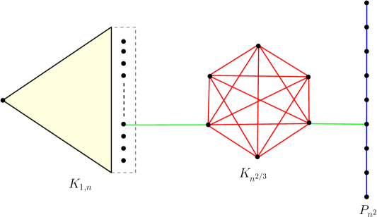
Figure 2. Illustration for Example 3.

Example 3.

Let $G_{n}$ be the graph in Figure 2. Note that it has three parts, a $K_{1,n}$, where one of the leaves is connected by a single edge to a $K_{n^{2/3}}$, which is connected by a single edge to a path $P_{n^{2}}$. Consider coloring this graph by $c_{n}$ colors such that $c_{n}/n\rightarrow\kappa$. This implies

$$\mathbb{E}(T(K_{1,2},G_{n}))=\frac{1}{c_{n}^{2}}N(K_{1,2},G_{n})\sim\frac{{n\choose 2}+3{\lceil n^{2/3}\rceil\choose 3}+n^{2}}{c_{n}^{2}}\rightarrow 2\kappa^{2}.$$

Next, note that $\Delta(G_{n})=n$, which corresponds to the central vertex of the $K_{1,n}$. Therefore, $\theta_{1}=\kappa$. For every other vertex the degree is $o(n)$, which implies $\theta_{v}=0$, for all $v\geq 2$. Finally, since $N(K_{3},G_{n})={\lceil n^{2/3}\rceil\choose 3}$, $\nu:=\lim_{n\rightarrow\infty}\frac{1}{c_{n}^{2}}N(K_{3},G_{n})=\frac{\kappa^{2}}{6}$. Therefore, by Theorem 1.2

$$T(K_{1,2},G_{n})\stackrel{{\scriptstyle D}}{{\to}}{T_{1}\choose 2}+3Z_{3}+Z_{1},$$

where $T_{1}\sim\operatorname{Pois}(\kappa)$, $Z_{3}\sim\operatorname{Pois}(\frac{\kappa^{2}}{6})$, and $Z_{1}\sim\operatorname{Pois}(\frac{\kappa^{2}}{2})$.

Remark 3.1.

(Extension to random graphs) By a simple conditioning argument, Theorem 1.2 can be extended to random graphs by conditioning on the graph, under the assumption that the graph and its coloring are jointly independent (see [4, Lemma 4.1]). In this case, whenever the limits in (1.4) and (1.6) exist in probability, the limit (1.7) holds. For example, when $G_{n}\sim G(n,p(n))$ is the Erdős-Rényi random graph, then the limiting distribution of $T(K_{1,r},G_{n})$ (when $c_{n}$ is chosen such that $\frac{1}{c_{n}^{r}}\mathbb{E}(N(K_{1,r},G_{n}))\rightarrow\lambda$) can be easily derived using Theorem 1.2. In this case, depending on whether (a) $n^{\frac{r+1}{r}}p(n)\rightarrow O(1)$, (b) $p(n)\rightarrow 0,n^{\frac{r+1}{r}}p(n)\rightarrow\infty$, or (c) $p(n)=p\in(0,1)$ is fixed, $T(K_{1,r},G_{n})$ converges to (a) zero in probability, or (b) $\operatorname{Pois}(\lambda)$, or (c) a linear combination of independent Poisson variables (see [4, Theorem 1.3] for details).

4. Conclusion and Open Problems

This paper studies the limiting distribution of the number of monochromatic $r$-stars in a uniformly random coloring of a growing graph sequence. We provide a complete characterization of the limiting distribution of $T(K_{1,r},G_{n})$, in the regime where $\mathbb{E}(T(K_{1,r},G_{n}))=\Theta(1)$.

It remains open to understand the limiting distribution of $T(K_{1,r},G_{n})$ when $\mathbb{E}(T(K_{1,r},G_{n}))=\frac{1}{c_{n}^{2}}N(K_{1,r},G_{n})$ grows to infinity. For the case of monochromatic edges, [3, Theorem 1.2] showed that $T(K_{2},G_{n})$ (centered by the mean and scaled by the standard deviation) converges to $N(0,1)$, whenever $\mathbb{E}(T(K_{2},G_{n}))=\frac{1}{c_{n}}|E(G_{n})|\rightarrow\infty$ such that $c_{n}\rightarrow\infty$. Error rates for the above CLT were obtained by Fang [13]. It is natural to wonder whether this universality phenomenon extends to monochromatic $r$-stars, and more generally, to any fixed connected graph $H$.

On the other hand, when $\mathbb{E}(T(K_{2},G_{n}))\rightarrow\infty$ such that the number of colors $c_{n}=c$ is fixed, then $T(K_{2},G_{n})$ (after appropriate centering and scaling) is asymptotically normal if and only if its fourth moment converges to 3 [3, Theorem 1.3]. It would be interesting to explore whether this fourth-moment phenomenon extends to monochromatic $r$-stars.

Acknowledgement: The authors are indebted to Somabha Mukherjee for his careful comments on an earlier version of the manuscript, and Swastik Kopparty for helpful discussions.

References

- [1] A. D. Barbour, L. Holst, and S. Janson, Poisson Approximations, Oxford University Press, Oxford, 1992.
- [2] A. Basak and S. Mukherjee, Universality of the mean-field for the Potts model, Probability Theory and Related Fields, to appear, 2017.
- [3] B. B. Bhattacharya, P. Diaconis, and S. Mukherjee, Universal Poisson and Normal limit theorems in graph coloring problems with connections to extremal combinatorics, Annals of Applied Probability, Vol. 27 (1), 337–394, 2017.
- [4] B. B. Bhattacharya, S. Mukherjee, and S. Mukherjee, Birthday paradox, monochromatic subgraphs, and the second moment phenomenon, arXiv:1711.01465, 2017.
- [5] B. B. Bhattacharya and S. Mukherjee, Monochromatic subgraphs in randomly colored graphons, arXiv:1707.05889, 2017.
- [6] A. Cerquetti and S. Fortini, A Poisson approximation for colored graphs under exchangeability, Sankhya: The Indian Journal of Statistics Vol. 68(2), 183–197, 2006.
- [7] S. Bhamidi, J. M. Steele, and T. Zaman, Twitter event networks and the Superstar model, Annals of Applied Probability, 25 (5), 2462–2502, 2015.
- [8] S. Chatterjee, P. Diaconis, and E. Meckes, Exchangeable pairs and Poisson approximation, Electron. Encyclopedia Probab., 2004.
- [9] A. DasGupta, The matching, birthday and the strong birthday problem: a contemporary review, J. Statist. Plann. Inference, Vol. 130, 377–389, 2005.
- [10] P. Diaconis and S. Holmes, A Bayesian peek into Feller I, Sankhya, Series A, Vol. 64 (3), 820–841, 2002.
- [11] P. Diaconis and F. Mosteller, Methods for studying coincidences, The Journal of the American Statistical Association, Vol. 84(408), 853–861, 1989.
- [12] F. M Dong, K. M. Koh, and K. L. Teo, Chromatic polynomials and chromaticity of graphs, World Scientific Publishing Company, 2005.
- [13] X. Fang, A universal error bound in the CLT for counting monochromatic edges in uniformly colored graphs, Electronic Communications in Probability, Vol, 20, Article 21, 1–6, 2015.
- [14] J. H. Friedman and L. C. Rafsky, Multivariate generalizations of the Wolfowitz and Smirnov two-sample tests, Annals of Statistics, Vol. 7, 697–717, 1979.
- [15] S. D. Galbraith, M. Holmes, A non-uniform birthday problem with applications to discrete logarithms, Discrete Applied Mathematics, Vol. 160 (10-11), 1547–1560, 2012.
- [16] T. R. Jensen and B. Toft, Unsolved Graph Coloring Problems, In L. Beineke & R. Wilson (Eds.), Topics in Chromatic Graph Theory, Encyclopedia of Mathematics and its Applications, Cambridge University Press, 327–357, 2015.
- [17] R. P. Stanley, A symmetric function generalization of the chromatic polynomial of a graph, Advances in Mathematics, Vol. 111 (1), 166–194, 1995.