Spontaneous Spin Polarization due to Tensor Selfenergies in Quark Matter

Abstract

We study the magnetic properties of quark matter in the NJL model with the tensor interaction. The spin-polarized phase given by the tensor interaction remains even when the quark mass is zero, while the phase given by the axial vector interaction disappears. There are two kinds of spin-polarized phases: one appears in the chiral-broken phase, and the other appears in the chiral-restored phase where the quark mass is zero. The latter phase can appear independently of the strength of the tensor interaction.

I Introduction

Discovery of magnetars mag3 ; mag , which are neutron stars with super strong magnetic field, seems to revive an important question about the origin of the strong magnetic field in compact stars. Magnetars have huge magnetic field of 10¹⁵G and are grouped into a new class of compact stars. Many people usually assume the conservation of magnetic flux during the stellar evolution to explain the magnetic field of the pulsar. However, if we naively apply this hypothesis to magnetars, we immediately have a contradiction that their radius should be much less than the Schwarzschild radius. Thus, it may not be very easy to explain the strong magnetic field without considering properties of hadronic matter inside stars. We should pay attention to a microscopic origin to solve the “magnetar” problem,

Recently, many theoretical and experimental efforts have been devoted to explore the QCD phase diagram in the density-temperature plane, which may be closely related to phenomena observed in relativistic heavy-ion collisions, compact stars or early universe R-ion ; R-star ; R-star2 . In particular, quark-gluon plasma (QGP) at high-temperature but low-density regime and color superconductivity (CSC) at high-density and low-temperature regime have been elaborately studied R-ion ; csc .

Because dense matter occupies a large portion of compact stars, its property should be reflected in various phenomena. In Ref. tat00 one of the author (T.T.) has suggested a possibility of a ferromagnetic transition in QCD; it is possible in quark matter interacting with one-gluon-exchange interaction and its critical density is order of nuclear density, $\rho_{FM}\simeq\rho_{0}$, where $\rho_{0}$ is normal nuclear matter density. Using this idea we can roughly estimate the strength of the magnetic field at the surface of compact stars. Considering a star with mass, $M\sim 1.4M_{\odot}$, and radius, $R\sim 10$Km, and assuming the dipole magnetic field, the maximum strength at the surface can be simply estimated by $B_{\rm max}=(8\pi/3)f_{Q}\mu_{q}\rho_{0}$, where $f_{Q}$ is the volume fraction of quark matter and $\mu_{q}$ the quark magnetic moment. Thus we evaluate it as $O(10^{15-17}{\rm G})$ for the extreme case, $f_{Q}=1$, which should be compared with observations. This is a perturbative result based on the Bloch mechanism, in analogy with electron gas blo29 ; her66 ; mor85 .

In the relativistic framework the “spin density” can take the two forms MaruTatsu , $\psi^{\dagger}\Sigma^{i}\psi(\equiv-\mbox{${\bar{\psi}}$}\gamma_{5}\gamma^{i}\psi)$ and $\psi^{\dagger}\gamma^{0}\Sigma^{i}\psi(\equiv-\mbox{${\bar{\psi}}$}\sigma^{12}\psi)$, with $\psi$ being the quark field. The former is a space-component of the axial-vector (AV) mean-field, and the later is that of the tensor (T) one. These two mean-fields become equivalent to each other in the non-relativistic limit, while they are quite different in the ultra-relativistic limit (massless limit) MaruTatsu . In the text we shall call the former and latter polarization the AV-type and T-type spin polarizations (SP), respectively.

For quark matter, we have introduced the AV interaction and have studied the SP mechanism in the mean-field approximation tat00 ; NT05 ; MNT . In theses studied we have succeeded to show the co-existence of the spin polarization and the color super-conductivity (CSC) nak03A and the dual chiral density wave (DCDW) NT05 ; YT15 .

Furthermore, Maedan have also studied the SP in the NJL model with this AV mean-field maedan07 . When the mass is fixed, the SP appears in high density region, but the AV mean-field disappears when the quark mass becomes zero. Then, the spin-polarized phase can appear in small density region just lower than the chiral phase transition density.

As mentioned above, the AV channel of two quark interaction has often been used for the SP study in quark matter because this channel is obtained by the Fierz transformation from the one-gluon exchange (OGE) interaction. On the other hand, the T channel has not been often used first because this interaction channel does not appear in the Fierz transformation from the OGE interaction. However, low-energy effective QCD models such as the NJL model have not been constructed based on the OGE interaction, and there is not any reason to exclude this channel.

The T channel interaction can play an important role differently from the AV channel interaction to produce the spin-polarized phase because the T-type SP can appear even if the quark mass becomes zero MNT . Actually, Tsue et al. TPPY has also shown that the SP appears in the chiral-restored phase, where the quark mass is zero, in the NJL model within the effective potential approach.

In addition, the magnetic interaction of quark matter with the T-type SP is much larger than that of the AV-type SP MNT . In the Fermi degenerate system, the magnetic field should be almost created by magnetization, which is proportional to $\psi^{\dagger}\gamma^{0}\Sigma^{i}\psi$. The lower component of the Dirac spinor contributes to $\psi^{\dagger}\Sigma^{i}\psi$ and $\psi^{\dagger}\gamma^{0}\Sigma^{i}\psi$, oppositely. In the relativistic region, where the quark mass is much less than the Fermi momentum, the contribution from the lower component has the same order of that from the upper component. As $<\psi^{\dagger}\Sigma^{i}\psi>$ increases, then, $<\psi^{\dagger}\gamma^{0}\Sigma^{i}\psi>$ becomes smaller in the AV-type SP.

Thus, the AV-type SP appears in narrow density region below the chiral transition and may not contribute to the magnetic field very largely. In contrast, the T-type SP can appear in the wide density region and largely contribute to the magnetic field. Thus, we should examine behaviors of the SP and its relation with chiral symmetry.

In this paper we study the T-type SP in the NJL model and figure out the relation between the spontaneous SP and chiral transition. In the next section we present a framework to deal with the present subject. In Sec. 3 we show the results of the numerical calculation and discuss the relation between SP and chiral restoration. Sec. 4 is devoted to summary and concluding remarks.

II Formalism

II.1 Lagrangian and Quark Propagator

In order to examine the T-type SP we start with the following NJL-type Lagrangian density with $SU(2)$ chiral symmetry,

$${\cal L}={\cal L}_{K}+{\cal L}_{s}+{\cal L}_{V}+{\cal L}_{T}$$ (1)

with

$${\cal L}_{K} = \mbox{${\bar{\psi}}$}(i\mbox{\ooalign{\hfil/\hfil\crcr{$\partial$}}}-m)\psi,$$ (4)

$${\cal L}_{S} = -\frac{G_{s}}{2}\left[(\mbox{${\bar{\psi}}$}\psi)^{2}+(i\mbox{${\bar{\psi}}$}\gamma_{5}\tau\psi)^{2}\right],$$ (5)

$${\cal L}_{V} = -\frac{G_{v}}{2}\left[(\mbox{${\bar{\psi}}$}\gamma_{\mu}\psi)(\mbox{${\bar{\psi}}$}\gamma^{\mu}\psi)+(i\mbox{${\bar{\psi}}$}\gamma_{5}\gamma_{\mu}\tau\psi)(i\mbox{${\bar{\psi}}$}\gamma^{\mu}\gamma_{5}\tau\psi)\right],$$ (6)

$${\cal L}_{T} = -\frac{G_{T}}{2}\left[(\mbox{${\bar{\psi}}$}\sigma_{\mu\nu}\psi)(\mbox{${\bar{\psi}}$}\sigma^{\mu\nu}\psi)+(\mbox{${\bar{\psi}}$}i\tau_{a}\gamma_{5}\sigma_{\mu\nu}\psi)(\mbox{${\bar{\psi}}$}i\tau_{a}\sigma^{\mu\nu}\gamma_{5}\psi)\right],$$ (7)

where $\psi$ is a field operator of quark, $G_{s}$, $G_{v}$ and $G_{T}$ are the coupling constants for the scalar, vector and tensor channels, respectively.

Here, we comment on the tensor interaction. If the original Lagrangian includes only ${\cal L}_{S}$ in Eq. (5), the Fierz transformation effectively gives the following Lagrangian:

$${\cal L}_{FT} = \frac{1}{4}G_{s}\left[\left(\mbox{${\bar{\psi}}$}\psi\right)^{2}+\left(\mbox{${\bar{\psi}}$}i\tau\gamma_{5}\psi\right)^{2}-\left(\mbox{${\bar{\psi}}$}\tau\psi\right)^{2}-\left(\mbox{${\bar{\psi}}$}i\gamma_{5}\psi\right)^{2}+2\left(\mbox{${\bar{\psi}}$}\gamma_{5}\gamma_{\mu}\psi\right)\left(\mbox{${\bar{\psi}}$}\gamma_{5}\gamma^{\mu}\psi\right)\right.$$ (8)

$$\left.-2\left(\mbox{${\bar{\psi}}$}\gamma_{\mu}\psi\right)\left(\mbox{${\bar{\psi}}$}\gamma^{\mu}\psi\right)+\frac{1}{2}\left(\mbox{${\bar{\psi}}$}\sigma_{\mu\nu}\psi\right)\left(\mbox{${\bar{\psi}}$}\sigma^{\mu\nu}\psi\right)-\frac{1}{2}\left(\mbox{${\bar{\psi}}$}\sigma_{\mu\nu}\tau\psi\right)\left(\mbox{${\bar{\psi}}$}\sigma^{\mu\nu}\tau\psi\right)\right].$$

Thus, the T channel of the interaction can appear even if the original interaction does not include this channel.

In the present work, we restrict calculations and discussions to the flavor symmetric matter ($\rho_{u}=\rho_{d}$) at zero temperature. Within the mean-field approximation the quark Dirac spinor $u({\mbox{$\bm{p}$},s})$ is obtained as the solution of the following equation,

$$\left[\mbox{\ooalign{\hfil/\hfil\crcr$p$}}-M_{q}-U_{0}\gamma^{0}-U_{T}\Sigma_{z}\right]u(\mbox{$\bm{p}$},s)=0$$ (9)

with $\Sigma_{z}={\rm diag}(1,-1,1,-1)$ and

$$M_{q} = -G_{s}\rho_{s}=-G_{s}<\mbox{${\bar{\psi}}$}\psi>,$$ (10)

$$U_{0} = G_{v}\rho_{q}=G_{v}<\mbox{${\bar{\psi}}$}\gamma^{0}\psi>,$$ (11)

$$U_{T} = G_{T}\rho_{T}=G_{T}<\mbox{${\bar{\psi}}$}\Sigma_{z}\psi>-G_{T}<\mbox{${\bar{\psi}}$}\Sigma_{z}\tau_{3}\psi>\tau_{3}.$$ (12)

In the mean-field approximation the quark Green function is defined as a solution of the following equation:

$$\left[\mbox{\ooalign{\hfil/\hfil\crcr$p$}}-M_{q}-U_{0}\gamma^{0}-U_{T}\Sigma_{z}\right]S(p)=1.$$ (13)

By solving the above Eq. (13) we can obtain

$$S(p)=\frac{\left[\gamma_{\mu}p^{*\mu}+M_{q}+\Sigma_{z}U_{T}\right]\left\{p^{*2}-M_{q}^{2}+U_{T}^{2}+2U_{T}(p_{z}\gamma_{5}\gamma^{0}-p_{0}\gamma_{5}\gamma^{3})\right\}}{(p_{0}^{*2}-E_{p}^{2}-U_{T}^{2})^{2}-4U_{T}^{2}(\mbox{$\bm{p}$}_{T}^{2}+M_{q}^{2})\pm i\delta}$$ (14)

with $p_{\mu}^{*}=p_{\mu}-U_{0}\delta^{0}_{\mu}$ and $E_{p}=\sqrt{\mbox{$\bm{p}$}^{2}+M_{q}^{2}}$.

The $S(p)$ has poles at $p_{0}=\pm e(\mbox{$\bm{p}$},s)$, which give single particle energies

$$e(\mbox{$\bm{p}$},s)=\sqrt{(\sqrt{M_{q}^{2}+\mbox{$\bm{p}$}_{T}^{2}}+sU_{T})^{2}+p_{z}^{2}}+U_{0}=\sqrt{E_{p}^{2}+2sU_{T}\sqrt{M_{q}^{2}+\mbox{$\bm{p}$}_{T}^{2}}+U_{T}^{2}}+U_{0},$$ (15)

where $s=\pm 1$ indicates the spin of a quark.

It should be interesting to compare it with a single particle energy in the AV mean-field, $U_{A}$:

$$e(\mbox{$\bm{p}$},s)=\sqrt{(\sqrt{M_{q}^{2}+p_{z}^{2}}+sU_{A})^{2}+\mbox{$\bm{p}$}_{T}^{2}}+U_{0}=\sqrt{E_{p}^{2}+2sU_{A}\sqrt{M_{q}^{2}+p_{z}^{2}}+U_{A}^{2}}+U_{0}.$$ (16)

Here, we make a comment on the difference in the SP between the tensor and axial-vector interactions. When $U_{A}=U_{T}$, we can obtain the above expression of $e(\mbox{$\bm{p}$},s)$ in Eq. (16) from that in Eq. (15) by exchanging $p_{z}$ and $p_{T}$. The surfaces in the momentum space at the fixed energy have the same relation between the two types of SP. However, $p_{z}$ is one-dimensional while $p_{T}$ is the absolute value of the two dimensional vector.

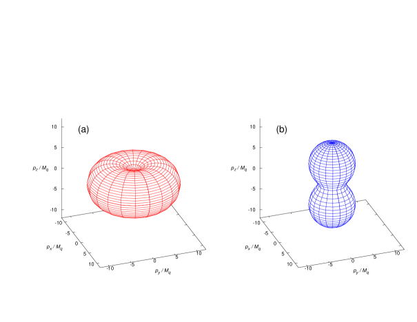
Figure 1: The energy constant surfaces for $e-U_{0}=3M_{q}$ and $s=-1$, when $U_{T}=3M_{q}$ (a) and when $U_{A}=3M_{q}$ (b).

In Fig. 1, we show the constant energy surface for $e(\mbox{$\bm{p}$},-1)-U_{0}=3M_{q}$ in the T-Type spin-polarized phase when $U_{T}=3M_{q}$ (a) and in the AV-type spin-polarized phase when $U_{A}=3M_{q}$ (b). We see that difference in the momentum distribution between the two types of the SP: it is deformed prolately in the T-type SP and oblately in the AV-Type SP.

Using these single particle energies, the quark propagator is separated into the vacuum part $S_{F}$ and the density dependent part $S_{D}$ as

$$S(p)=S_{F}(p)+S_{D}(p).$$ (17)

with

$$S_{F}(p) = \frac{\left[\gamma^{\mu}p^{*}_{\mu}+M_{q}+\Sigma_{z}U_{T}\right]\left\{p^{2}-M_{q}^{2}+U_{T}^{2}+2U_{T}(p_{z}\gamma_{5}\gamma^{0}-p_{0}\gamma_{5}\gamma^{3})\right\}}{\left[p_{0}^{2}-e^{*2}(\mbox{$\bm{p}$},1)+i\delta\right]\left[p_{0}^{2}-e^{*2}(\mbox{$\bm{p}$},-1)+i\delta\right]},$$ (18)

$$S_{D}(p) = \sum_{s=\pm 1}\left[\gamma_{0}e^{*}-\mbox{$\bm{\gamma}$}\cdot\mbox{$\bm{p}$}+M_{q}+\Sigma_{z}U_{T}\right]\left\{1+\frac{s(p_{z}\gamma_{5}\gamma^{0}-p_{0}\gamma_{5}\gamma^{3})+sU_{T}}{\sqrt{\mbox{$\bm{p}$}_{T}^{2}+M_{q}^{2}}}\right\}$$ (19)

$$\quad\quad\times\frac{i\pi}{2e^{*}(\mbox{$\bm{p}$},s)}n(\mbox{$\bm{p}$},s)\delta[p_{0}-e(\mbox{$\bm{p}$},s)],$$

where $p^{*}_{\mu}-p_{\mu}-U_{0}\delta^{0}_{\mu}$, $e^{*}=e-U_{0}$, $n(\mbox{$\bm{p}$},s)=\Theta[e_{F}-e(\mbox{$\bm{p}$},s)]$, and $e_{F}$ is the Fermi energy.

In the above expression, the quark density is written as

$$\rho_{q} = N_{d}\sum_{s=\pm 1}\int\frac{d^{3}p}{(2\pi)^{3}}\theta[e_{F}-e(\mbox{$\bm{p}$},s)],$$ (20)

where $N_{d}=N_{f}N_{c}=6$ is given by the degeneracy of the flavors, $N_{f}=2$, and color degrees of freedom, $N_{c}=3$; the baryon density is given as $\rho_{B}=\rho_{q}/N_{c}$.

Here, we give a comment about the vector channel of the interaction. The vector mean-field, $U_{0}$, has only a role to shift the single particle energy and does not influence a spin property. Without $U_{0}$, the quark chemical potential, $e_{F}$, does not monotonously increase as density becomes larger. The system transits from the density with the maximum chemical potential to the chiral restoration; this transition is the first order phase transition. As the $G_{v}$ increases, the transition density becomes larger, and, when the vector field is sufficiently large, the phase transition is of the second order TMF91 ; MTF92 .

Thus, we can control the phase transition with the vector interaction without changing magnetic properties. We assume that the vector coupling $G_{v}$ is large, and that the chiral transition is of the second order. We rewrite $p_{0}^{*}$ and $e^{*}$ to $p_{0}$ and $e$ and eliminate $U_{0}$ in the following.

In the mean-field approximation the dynamical quark mass $M_{q}$ and the $U_{T}$ are determined by

$$1-\frac{G_{s}\rho_{s}}{M_{q}} = 0,$$ (21)

$$1-\frac{G_{T}\rho_{T}}{U_{T}} = 0,$$ (22)

where the scalar density $\rho_{s}$ and the tensor density are given by

$$\rho_{s} = N_{d}\int\frac{d^{4}p}{(2\pi)^{4}}{\rm Tr}\left[iS(p)\right],$$ (23)

$$\rho_{T} = N_{d}\int\frac{d^{4}p}{(2\pi)^{4}}{\rm Tr}\left[i\Sigma_{z}S(p)\right].$$ (24)

The scalar density is separated into two parts, the vacuum part and the density-dependent part as

$$\rho_{s}=\rho_{s}(V)+\rho_{s}(D)=N_{d}\int\frac{d^{4}p}{(2\pi)^{4}}{\rm Tr}\left[iS_{F}(p)\right]+N_{d}\int\frac{d^{4}p}{(2\pi)^{4}}{\rm Tr}\left[iS_{D}(p)\right].$$ (25)

The density dependent part is written as

$$\rho_{s}(D) = N_{d}\sum_{s=\pm 1}\int\frac{d^{3}p}{(2\pi)^{3}}~{}n(\mbox{$\bm{p}$},s)~{}\frac{M_{q}}{e(\mbox{$\bm{p}$},s)}\left(1+\frac{sU_{T}}{\sqrt{M_{q}^{2}+p_{T}^{2}}}\right).$$ (26)

The density dependent part of the tensor density is also written as

$$\rho_{T}(D) = N_{d}\sum_{s=\pm 1}\int\frac{d^{3}p}{(2\pi)^{3}}~{}n(\mbox{$\bm{p}$},s)~{}\frac{s\sqrt{\mbox{$\bm{p}$}_{T}^{2}+M_{q}^{2}}+U_{T}}{e(\mbox{$\bm{p}$},s)}.$$ (27)

Because $\rho_{T}<0$ when $U_{T}>0$, so that Eq. (22) has a solution when $G_{T}<0$.

This argument is right only when the SP is isoscalar, where the average spin of u- and d-quarks are directed along the same direction. In the isovector spin-polarized system the tensor densities for u- and d-quark have opposite signs. In the symmetric matter, we define $\rho_{T}=\rho_{T}(u)-\rho_{T}(d)=2\rho_{T}(u)$ and $U_{T}=U_{T}(u)-U_{T}(d)=2U_{T}(u)$, and rewrite Eq. (12) as $U_{T}=-G_{T}\rho_{T}$, which is the same as Eq. (22) except the sign of r.h.s. This fact demonstrates that, when $G_{T}>0$, the isovector spin-polarized phase can appear, and its strength is the same as that for $G_{T}<0$.

Here, we give a comment on the tensor density. When $M_{q}=0$, the tensor density in Eq. (27) becomes

$$\rho_{T}(D)=-\frac{N_{d}}{12\pi}e_{F}^{3}\neq 0,$$ (28)

while $\rho_{A}=0$ NT05 ; nak03A . When $M_{q}=0$, namely, the T-type SP can appear while the AV-type SP never appears. This difference comes from the momentum distribution in the SP phase (see Fig. 1).

In this paper we per form the argument only when $G_{T}<0$, but we can apply the same argument to the isovector spin-polarized system for $G_{T}>0$; the latter system has a larger magnetization because of the opposite sign for the u- and d-quark charges.

In order to extract the vacuum part we use the proper time regularization (PTR) SchPTR51 , where the thermodynamical potential density is written as

$$\Omega_{vac} = iN_{d}\int\frac{d^{4}p}{(2\pi)^{4}}\ln\left[(p_{0}^{2}-e^{2}(\mbox{$\bm{p}$},+1))\right]\left[(p_{0}^{2}-e^{2}(\mbox{$\bm{p}$},-1))\right]$$ (29)

$$= -iN_{d}\sum_{s=\pm 1}\int_{0}^{\infty}\frac{d\tau}{\tau}\int\frac{d^{4}p}{(2\pi)^{4}}e^{\tau\left[(p_{0}^{2}-e^{2}({\bf p},s))\right]}$$

$$\approx \frac{N_{d}}{8\pi^{2}}\sum_{s}\int_{1/\Lambda^{2}}^{\infty}\frac{d\tau}{\tau^{2}}\int_{M_{q}}^{\infty}dE_{T}E_{T}e^{-\tau(E_{T}+sU_{T})^{2}}$$

at zero temperature, where $\Lambda$ is the cut-off parameter. The vacuum part of the scalar density is then given by

$$\rho_{s}(V)=\frac{\partial\Omega_{vac}}{\partial M_{q}~{}~{}}=-\frac{N_{d}M_{q}}{8\pi^{2}}\sum_{s}\int_{1/\Lambda^{2}}^{\infty}\frac{d\tau}{\tau^{2}}e^{-\tau(M_{q}+sU_{T})^{2}}=-\frac{N_{d}M_{q}}{8\pi^{2}}\Lambda^{2}\sum_{s}F_{2}\left(\frac{(M_{q}+sU_{T})^{2}}{\Lambda^{2}}\right),$$ (30)

where the function $F_{n}$ is defined as

$$F_{n}(x)=x\int_{x}^{\infty}\frac{d\tau}{\tau^{n}}e^{-\tau}.$$ (31)

The vacuum part of the tensor density can be also obtained with $\rho_{T}(V)=\partial\Omega_{vac}/\partial U_{T}$. However, this term strongly depends on the cut-off parameter $\Lambda$ in the present model, even when $M_{q}=0$. Indeed, the vacuum part of the tensor density is also dependent on the regularization scheme and the value of the cut-off parameter. (see Appendix.B.1 for details). For example, the vacuum contribution in the PTR suppresses the SP while that in the effective potential approach TPPY enlarges it.

In the AV type SP, the vacuum part in the PTR also suppresses the SP NT05 , while that in the momentum cut-off enlarges it maedan07 .

The cut-off parameter has a role to restrict the momentum space in the calculation. The T and AV densities are given by the difference between the spin-up and spin-down contributions, which depends on the restriction of the momentum space, so that the result sensitively depends on the regularization method and the value of the cut-off parameter.

In the usual renormalization procedure we regularize the vacuum polarization by introducing the suitable counter terms which are determined from physical values. In order to regularize the tensor density, $\rho_{T}(V)$ we need to introduce at least three counter terms which are proportional to $U_{T}^{2}$, $U_{T}^{4}$ and $U_{T}^{2}M^{2}$. In the NJL model we regularize the vacuum contributions by using a cut-off parameter. The vacuum part of the scalar density is associated with the dynamical quark mass in the vacuum, but not concerned with the spin properties. In the present model, the vacuum part of the tensor density strongly diverges as $\Lambda\rightarrow\infty$ for small asymmetry of the spin states. This fact does not have any physical meaning, but we do not have any clear rule to regularize the tensor density in a systematic way.

Thus, the cut-off dependence of the tensor density from the vacuum contribution is less meaningful at present. In the NJL model it is not easy to apply a consistent method even for the qualitative discussions. In the next section, then, we perform actual calculation without the vacuum contribution for the tensor density: $\rho_{T}\approx\rho_{T}(D)$.

In Appendix B.2, instead, we try to give a temporal calculation for the SP including it.

III Results

In this section we show some numerical results for SP in relation with chiral restoration. For this purpose, we consider the chiral limit and use two kinds of the parameter-sets PM1 ($G_{s}\Lambda^{2}=6,\Lambda=850$ MeV) and PM2 ($G_{s}\Lambda^{2}=6.35,\Lambda=660.37$ MeV) from Ref. NT05 .

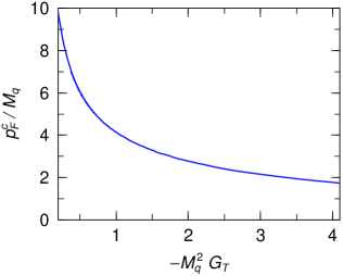
Figure 2: Coupling constant versus the critical Fermi momentum for the spontaneous spin polarization.

Before showing actual numerical results, we discuss the critical density of the SP ($\rho_{SC}$).

The tensor mean-field is determined by the following self-consistent equation :

$$F_{T}(U_{T})=1-\frac{G_{T}\rho_{T}}{U_{T}}=0.$$ (32)

When $U_{T}\gg e_{F}+M_{q}$, $\rho_{T}=-N_{d}e_{F}^{3}/12\pi$ and $\rho_{q}=N_{d}U_{T}e_{F}^{2}/4\pi$ (see Sec. A), so that $e_{F}\rightarrow 0$ and $F_{T}(U_{T})\rightarrow 1$ when $U_{T}\rightarrow\infty$ at the fixed density. Hence, Eq. (32) has a solution when $F_{T}(0)<0$ at $U_{T}=0$ which leads to

$$J=1+\frac{G_{T}N_{d}}{2\pi^{2}}\left\{p_{F}E_{F}+\frac{M_{q}^{2}}{2}\ln\left(\frac{E_{F}+p_{F}}{E_{F}-p_{F}}\right)\right\}\leq 0,\quad$$ (33)

where $p_{F}$ is the Fermi momentum, and $E_{F}=e_{F}(U_{T}=0)=\sqrt{p_{F}^{2}+M_{q}^{2}}$.

$J=0$ in Eq.(33) can be expressed by the two independent parameters, $M_{q}^{2}G_{T}$ and $p_{F}^{c}/M_{q}$, where $p_{F}^{c}$ indicates the critical Fermi momentum for the spontaneous SP. We show the boundary of the spin-polarized phase in Fig. 2.

In Fig. 3 we show $F_{T}(0)$ with PM1 (a) and PM2 (b) when $-G_{T}/G_{s}=0.6\sim-1.5$ as functions of baryon density, $\rho_{B}$, normalized by the normal nuclear density $\rho_{0}=0.17$fm^-3. In addition, we show the dynamical quark mass normalized by nucleon mass $M_{N}$ at the spin-saturated system ($\rho_{T}=0$) with PM1 (solid line) and PM2 (long dashed line).

As baryon density becomes larger, $F_{T}(0)$ decreases at first, and increases later. so that $F_{T}(0)$ has a maximum at the chiral phase transition (CPT) density, $\rho_{c}$, and monotonously decreases, again.

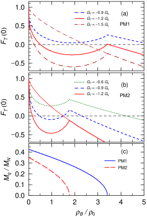
Figure 3: (Color online) $F_{T}(0)$ with PM1 (a) and PM2 (b) and the dynamical quark mass (c) as functions of $\rho_{B}/\rho_{0}$. In the upper (a) and middle (b) panels the dotted, dashed, solid and dot-dashed lines represent the results when $G_{T}/G_{s}=-0.6$, $-1.2$ and $-1.5$, respectively. The thin lines in the upper (a) and middle panels (b) indicates $F_{T}(0)$ when $M_{q}=0$. In the lower panel (c) the solid and long dashed lines indicate $M_{q}/M_{N}$ with PM1 and PM2, respectively.

It was shown in Ref. MNT that $F_{T}(0)$ monotonously decreases when the dynamical quark mass $M_{q}$ is fixed. However, the dynamical quark mass is also decreasing in the NJL model, and this effect enlarges $F_{T}$ up to $\rho_{B}=\rho_{c}$, where the quark dynamical mass becomes zero.

For comparison, we show $F_{T}(0)$ when $M_{q}=0$ with thin lines, where we plot the results only when $G_{T}=-1.5G_{s}$ for PM1 and $G_{T}=-1.2G_{s}$ for PM2. We see that $F_{T}(0)$ monotonously decreases when $M_{q}=0$ with the increase of $\rho_{B}$. Because $\partial M_{q}/\partial\rho_{B}$ is not continuous, the maximum point of $F_{T}(0)$ becomes a cusp, which corresponds to that the CPT is of the second order.

As mentioned before, $F_{T}(0)=0$ shows the critical density of the phase transition between the spin-saturated and spin-polarized phases. As the coupling $-G_{T}$ becomes larger, the number of the crossing points turns to be one, three and one. The last case, where the number of the crossing point is one, indicates that with $F_{T}(0)<0$ at $\rho_{B}=\rho_{c}$. In this case the line of $F_{T}(0)$ with $M_{q}=0$ also crosses zero at the density lower than the CPT density (see thin lines in Fig. 3).

These results suggest that there are two kinds of the spin-polarized phases: one is the chiral-broken SP (SP-I) which appears in the chiral-broken phase, $M_{q}>0$, and the other is the chiral-restored SP (SP-II) which appears in the chiral-restored phase, $M_{q}=0$. Here we define $\rho_{SC}^{({\rm I})}$ and $\rho_{SC}^{({\rm II})}$ as critical densities of the SP-I and SP-II phases, respectively. $\rho_{SC}^{({\rm II})}$ exits with any $G_{T}$, but $\rho_{SC}^{({\rm I})}$ appears only when $-G_{T}$, is large, namely the SP-II phase always appears independently of the strength of the tensor interaction. In addition, ${-G_{T}}$ becomes further larger, $F_{T}(0)<0$ at $\rho_{B}=\rho_{c}$ $\mbox{$\rho_{SC}^{({\rm II})}$}<\rho_{c}$; here, we should note that $M_{q}=0$ is a solution of Eq. (10) as well as a solution of the gap equation (21).

In Fig. 4, we show the baryon density dependence of the tensor density $\rho_{T}/\rho_{0}$ with PM1 (upper panel) and that of the dynamical mass (lower panel) when $G_{T}=-1.2G_{s}$ (a,b) and $G_{T}=-1.5G_{s}$ (c,d). In the upper panel the solid lines represent $\rho_{T}/(N_{c}\rho_{0})$ in the spin-polarized phase when $M_{q}>0$, and the dotted lines indicates that when $M_{q}=0$. In the lower panel, the solid and dashed lines represent the dynamical quark mass in the spin-polarized and spin-saturated phases, respectively.

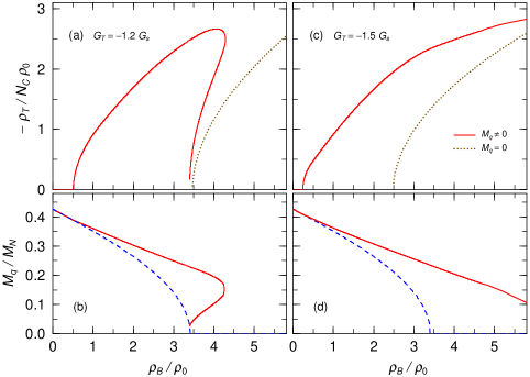
Figure 4: Spin polarization properties with PM1. Upper panels (a,c) : the tensor densities normalized by the normal nuclear density. The solid and dotted lines represent the results in the chiral symmetry broken and restored phases, respectively. Lower panels (b,d): the dynamical quark mass normalized by nucleon mass in the spin-polarized (solid lines) and spin-saturated phases (dashed line). The left and right panes show the results when $G_{T}=-1.2$ (a, b), $=-1.5$ (c, d), respectively.

When $G_{T}=-1.2G_{s}$ (a,b), we can see that two kinds of spin-polarized phases, SP-I and SP-II phases, appear. In addition, there are density region where the three solutions corresponding to the spin-polarized phases, two SP-I phases and one SP-II phase, exist.

When $G_{T}=-1.5G_{s}$ (c,d), the SP-I phase appears at first, and the SP-II phase appears in the density region, $\rho_{B}<\rho_{c}$. Both the two SP phases exist in a same density region up to a density larger than the CPT density, $\rho_{c}$, and the SP-I phase disappears at a density larger than $\rho_{c}$, where $M_{q}=0$ and $U_{T}\neq 0$.

In this approach we discard the vacuum contribution to the tensor density though the scalar density includes the vacuum part, so that we cannot define the total energy and cannot determine what is realized among the spin-saturated, SP-I and SP-II phases.

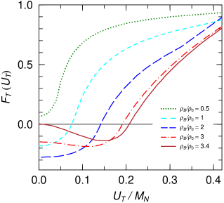
Figure 5: (Color online) $F_{T}(U_{T}))$ versus $U_{T}/M_{N}$ with PM1 and $G_{T}=-1.2G_{s}$. The dotted, dashed long-dashed, dot-dashed and solid lines represent results when $\rho_{B}/\rho_{0}=0.5,1,2,3,3.4$, respectively.

In order to look into this behavior more clearly, we calculate $F_{T}(U_{T})$ by varying baryon density. In Fig. 5 we show the results at several baryon densities.

When $\rho_{B}\lesssim 2\rho_{0}$, $F_{T}$ is a monotonously increasing function. As the density decreases, $F_{T}(0)$ becomes smaller, and, when $F_{T}(0)<0$, the equation $F_{T}(U_{T})=0$ has a solution.

When $\rho_{B}\gtrsim 2\rho_{0}$, $F_{T}(0)$ becomes larger with the increase of the density, but $F_{T}(U_{T})$ has a minimum at a certain $U_{T}$. The equation $F_{T}(U_{T})=0$ has two solutions when $F_{T}(0)>0$, and the minimum value is negative. As density further increases, the minimum value of $F_{T}$ becomes positive, and there is no solution.

In Fig. 6, we show the results with PM2 with $G_{T}=-0.8G_{s}$ (a,b), $G_{T}=-1.2G_{s}$ (c,d) and $G_{T}=-1.5G_{s}$ (e,f). The behaviors of the SP are similar to those in PM1 (Fig. 4). When $G_{T}=-0.8G_{s}$ (a,b), the SP-I and SP-II phases appear in different density region. When $G_{T}=-1.2G_{s}$ (c,d), and $G_{T}=-1.5G_{s}$ (e,f), the results clearly show that the SP-I and SP-II phases simultaneously exist in the density region, $\rho_{B}>\rho_{c}$, and that the SP-I phase disappears at higher density.

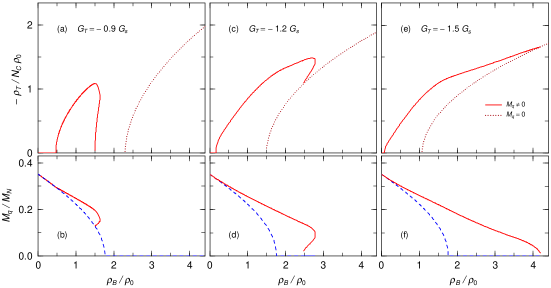
Figure 6: Spin polarization properties with PM2. Upper panels (a,c,e): the T densities normalized by the normal nuclear matter density. The solid and dotted lines represent the results in the chiral broken and restored phases, respectively. Lower panels (b,d,e): the dynamical quark mass normalized by nucleon mass in the spin-polarized (solid lines) and spin-saturated phase (dashed line). The left, middle and right panes show the results when $G_{T}/G_{s}=-0.9$ (a,b), $G_{T}/G_{s}=-1.2$ (c,d), $G_{T}/G_{s}=-1.5$ (e,f), respectively.

We can confirm that the SP-I phase disappears at a density larger than $\rho_{c}$, where the tensor density is finite, $\rho_{T}\neq 0$. In Fig. 7 we finally show the critical density between the spin-saturated and spin-polarized phases as a function of $G_{T}M^{2}_{N}$ in the chiral-broken phase, $\rho_{SC}^{({\rm I})}$, (a) and chiral-restored phase, $\rho_{SC}^{({\rm II})}$, (b). The critical density when $M_{q}=0$, $\rho_{SC}^{({\rm II})}$, is determined only by $G_{T}$, independently of $G_{s}$. In addition, we plot the critical density of CPT, $\rho_{c}$, with PM1 (dotted line) and PM2 (dashed line) in Fig. 7b.

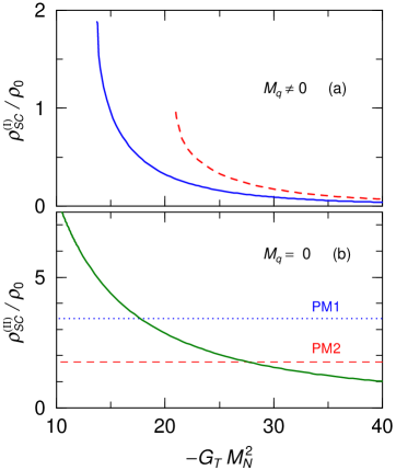
Figure 7: (Color Online) Critical density between the spin-saturated and spin-polarized phases as functions of $G_{T}M_{N}^{2}$ when $M_{q}\neq 0$ (a) and $M_{q}=0$ (b). In the upper panel the solid and dashed lines represent $\mbox{$\rho_{SC}^{({\rm I})}$}/\rho_{0}$ with PM1 and PM2, respectively. In the lower panel the solid line shows the critical density of SP-II, $\mbox{$\rho_{SC}^{({\rm II})}$}/\rho_{0}$, and the dotted and dashed lines indicate the critical densities of CPT, $\rho_{c}/\rho_{0}$, with PM1 and PM2, respectively.

We see the results in the chiral phase as follows. As $-G_{T}$ increases, the phase transition in the SP-I phase appears at $\rho_{B}\approx 1.9\rho_{0}$ when $-G_{T}M_{N}^{2}=13.8$ ($-G_{T}/G_{s}=0.949$) in PM1 and at $\rho_{B}\approx 0.96\rho_{0}$ when $-G_{T}M_{N}^{2}=21.0$ ($-G_{T}/G_{s}=0.819$) in PM2. In the chiral-restored phase $\mbox{$\rho_{SC}^{({\rm II})}$}\rightarrow\infty$ as $-G_{T}\rightarrow 0$, so that the phase transition occurs at any value of $-G_{T}$. As $-G_{T}$ increases, the critical density of SP-II, $\rho_{SC}^{({\rm II})}$, becomes smaller, and then it is lower than the CPT density, $\mbox{$\rho_{SC}^{({\rm II})}$}<\rho_{c}$, when $-G_{T}M^{2}>17.7$ ($G_{T}/G_{s}<-1.21$) in PM1 and when $-G_{T}M^{2}>27.6$ ($G_{T}/G_{s}<-1.07$) in PM2.

IV Summary

We have studied the spontaneous SP of quark matter in the NJL model with the tensor interaction. There appear two kinds of the spin-polarized phases, the SP-I and SP-II phases, where the dynamical quark mass is non-zero and zero, respectively. The SP-I phase appears when the T coupling $G_{T}$ is negatively large, but the SP-II phase can always appears above the critical density when $G_{T}<0$ though its transition density depends on $G_{T}$ MNT ; TPPY .

The SP-I phase can exist in the density region above the CPT density and shifts the chiral transition to higher density. On the other hand, the SP-II phase can appear below the CPT density. The SP-I and SP-II phases can exist at the same density when $-G_{T}$ is large. In the present model we cannot discuss the stability of each phase and make a critical conclusion. However, we can easily suppose that the phase transition between the SP-I and SP-II phases is of the first order.

We have considered an appearance of a non-uniform phase with the AV interaction during the chiral transition, where pseudo-scalar condensate as well as scalar condensate is non-vanishing, called as dual chiral density wave (DCDW) NT05 . The T-type SP must leads to a new type DCDW, which can appear in the chiral restored phase. We should study it in future.

In this paper we have made the discussion only when $G_{T}<0$: the spin-polarized phase is isoscalar. When $G_{T}>0$, the spin-polarized phase becomes isovector where the directions of the SP for $u$ and $d$ quarks are opposite. The strength of the magnetic field is much larger in the isovector spin-polarized phase than in the isoscalar SP phase because the charge of $u$ and $d$ quarks have opposite signs.

In the present work we have discarded the vacuum contribution to the tensor density because its contribution strongly depends on the regularization method. We have demonstrated in Appendix B that the vacuum contribution becomes important at high densities. However, the value of the cut-off parameter is determined to reproduce the dynamical quark mass in the vacuum, but is not related to the spin property, and then the large dependence on the cut-off parameter is not meaningful.

In order to remove the ambiguity we need to use a renormalizable model and to introduce counter terms to reproduce the vacuum spin-susceptibility at zero temperature, which is determined with the other model such as the lattice QCD. It is a future problem.

In this work, furthermore, we have not considered the AV channel of quark-quark interaction, which can be derived by the Fierz transformation of the one gluon exchange. The calculation of the spin-polarized phase is very difficult when both the T and AV interactions are introduced because the momentum distribution is very complicated. If the weak T interaction is mixed with the AV one, however, the AV-type SP phase appears even when the quark mass is zero; we have not discuss it in this paper.

When the quark mass is small, the tensor density decrease as the AV-type SP becomes larger , and the magnetic field which is produced by the spin-current also decreases MNT . However, the magnetic field can be kept to be finite by the tensor mean-field even if it is weak. So, the mixing of AV and T interactions may exhibit a new spin-polarization in quark matter.

In future, we hope to develop our formulation in the system including both the AV and T interactions.

Appendix A Density Dependent Parts of Densities

In this section, we give the detailed expressions of the quark density $\rho_{q}$ , the scalar density $\rho_{s}$ and the tensor density $\rho_{T}$ with the quark mass $M_{q}$, the chemical potential $e_{F}$ and the T field $U_{T}(>0)$.

A.1 Quark Densities

When $U_{T}<e_{F}-sM_{q}$ for $s=\pm 1$,

$$\rho_{q}(s) = \frac{N_{d}}{2\pi^{2}}\left\{\frac{1}{6}\sqrt{e_{F}^{2}-(M_{q}+sU_{T})^{2}}\left[2e_{F}^{2}-(M_{q}+sU_{T})(2M_{q}-sU_{T})\right]\right.$$ (34)

$$\left.\quad\quad-\frac{s}{2}U_{T}e_{F}^{2}\left[\frac{\pi}{2}-\sin^{-1}\left(\frac{M_{q}+sU_{T}}{e_{F}}\right)\right]\right\},$$

When $U_{T}>e_{F}-sM_{q}$,

$$\rho_{q}(+1)=0,\quad\rho_{q}(-1)=\frac{N_{d}}{4\pi}U_{T}e_{F}^{2}.$$ (35)

A.2 Scalar Densities

When $U_{T}<e_{F}-sM_{q}$ for $s=\pm 1$,

$$\rho_{s}(s) = \frac{N_{d}}{4\pi^{2}}M_{q}\left[e_{F}\sqrt{e_{F}^{2}-(M_{q}+sU_{T})^{2}}\right.$$ (36)

$$\quad\quad\quad\left.-\frac{(M_{q}+sU_{T})^{2}}{2}\ln\left(\frac{e_{F}+\sqrt{e_{F}^{2}-(M_{q}+sU_{T})^{2}}}{e_{F}-\sqrt{e_{F}^{2}-(M_{q}+sU_{T})^{2}}}\right)\right],$$

When $U_{T}>e_{F}-sM_{q}$,

$$\rho_{s}(\pm 1)=0,$$ (37)

A.3 Tensor Density

When $U_{T}<e_{F}-M_{q}$ for $s=1$ or $U_{T}<M_{q}$ for $s=-1$

$$\rho_{T}(s) = \frac{N_{d}}{12\pi^{2}}s\left\{(M_{q}+sU_{T})^{2}\left(-M_{q}+\frac{s}{2}U_{T}\right)\ln\left(\frac{e_{F}+\sqrt{e_{F}^{2}-(M_{q}+sU_{T})^{2}}}{e_{F}-\sqrt{e_{F}^{2}-(M_{q}+sU_{T})^{2}}}\right)\right.$$ (38)

$$\left.\quad\quad\quad\quad+~{}e_{F}(M_{q}-2sU_{T})\sqrt{e_{F}^{2}-(M_{q}+sU_{T})^{2}}\right.$$

$$\left.\quad\quad\quad\quad+e_{F}^{3}\sin^{-1}\left(\frac{\sqrt{e_{F}^{2}-(U_{T}+sM_{q})^{2}}}{e_{F}}\right)\right\}.$$

When $U_{T}>e_{F}-M_{q}$ for $s=1$,

$$\rho_{T}(+1)=0.$$ (39)

When $e_{F}+M_{q}>U_{T}>M_{q}$ for $s=-1$,

$$\rho_{T}(-1) = -\frac{N_{d}}{12\pi^{2}}\left\{-\frac{1}{2}(U_{T}-M_{q})^{2}\left(U_{T}+2M_{q}\right)\ln\left(\frac{e_{F}+\sqrt{e_{F}^{2}-(U_{T}-M_{q})^{2}}}{e_{F}-\sqrt{e_{F}^{2}-(U_{T}-M_{q})^{2}}}\right)\right.$$ (40)

$$\quad\quad\quad\quad+~{}e_{F}\left(2U_{T}+M_{q}\right)\sqrt{e_{F}^{2}-(U_{T}-M_{q})^{2}}$$

$$\left.\quad\quad\quad\quad+~{}e_{F}^{3}\left[\pi-\sin^{-1}\left(\frac{\sqrt{e_{F}^{2}-(U_{T}-M_{q})^{2}}}{e_{F}}\right)\right]\right\}.$$

When $U_{T}>e_{F}+M_{q}$ for $s=-1$,

$$\rho_{T}(-1) = -\frac{N_{d}}{12\pi}e_{F}^{3}.$$ (41)

Appendix B Vacuum Contribution to Tensor-Field

B.1 Ambiguities of Vacuum Contribution

In the text we mentioned that the vacuum contribution is ambiguous and dependent on the regularization scheme. We explain the reason of this difference with the energy cut-off and the three-dimensional momentum cut-off as examples.

In these regularization schemes, the vacuum part of the tensor density is written as

$$\rho_{T}(V)=N_{d}\int\frac{d^{4}p}{(2\pi)^{4}}{\rm Tr}\left[i\Sigma_{z}S_{F}(p)\right].$$ (42)

$$= iN_{d}\sum_{s}\int\frac{d^{4}p}{(2\pi)^{4}}n_{V}(\mbox{$\bm{p}$},s)\frac{4sU_{T}(-p_{0}^{2}-M^{2}-U_{T}^{2}-\mbox{$\bm{p}$}_{T}^{2}+p_{z}^{2})}{(-2e(\mbox{$\bm{p}$},s))[e^{2}(\mbox{$\bm{p}$},1)-e(\mbox{$\bm{p}$},-1)^{2}][p_{0}+e_{s}(\mbox{$\bm{p}$},s)-i\delta]},$$

$$= -N_{d}\sum_{s=\pm 1}\int\frac{d^{3}p}{(2\pi)^{3}}~{}n_{V}(\mbox{$\bm{p}$},s)~{}\frac{s\sqrt{\mbox{$\bm{p}$}_{T}^{2}+M_{q}^{2}}+U_{T}}{e(\mbox{$\bm{p}$},s)},$$

where $n_{V}(\mbox{$\bm{p}$},s)$ is an effective momentum distribution for negative energy particles including the cut-off parameter.

In the energy cut-off regularization, we should take $n_{V}=\Theta[\Lambda_{e}-e(\mbox{$\bm{p}$},s)]$; apparently the $\rho_{T}(V)$ is the different sign of $\rho_{T}(D)$; in the present choice $\rho_{T}(D)<0<\rho_{T}(V)$. Namely, the vacuum contribution suppresses the tensor density.

In general the cut-off parameter is taken to be much larger than the Fermi energy, $\Lambda_{e}\gg E_{F}$, and the total tensor density becomes positive, $\rho_{T}(V)+\rho_{T}(D)>0$, so that the SP does not appear when $G_{T}<0$. When $G_{T}>0$, however, the spontaneous SP appears in the vacuum when the cut-off, $\Lambda_{e}$, increases and exceeds a certain critical value; this phenomenon is not though to have any physical meaning.

In the momentum cut-off regularization, on the other hand, the effective momentum distribution is taken to be $n_{V}=\Theta(\Lambda_{p}-|\mbox{$\bm{p}$}|)$. When $0<U_{T}\ll 1$,

$$\rho_{T}(V) \approx -N_{d}\sum_{s=\pm 1}\int\frac{d^{3}p}{(2\pi)^{3}}~{}\Theta(\Lambda_{p}-|\mbox{$\bm{p}$}|)~{}\frac{s\sqrt{\mbox{$\bm{p}$}_{T}^{2}+M_{q}^{2}}+U_{T}}{E_{p}}\left(1-\frac{sU_{T}\sqrt{\mbox{$\bm{p}$}_{T}^{2}+M_{q}^{2}}}{E_{p}^{2}}\right),$$ (43)

$$\approx -2N_{d}U_{T}\int\frac{d^{3}p}{(2\pi)^{3}}~{}\Theta(\Lambda_{p}-|\mbox{$\bm{p}$}|)~{}\frac{p_{z}^{2}}{E_{p}^{3}}~{}<~{}0.$$

$\rho_{T}(V)$ has the same sign of $\rho_{T}(D)$, namely the vacuum contribution enlarges the tensor density.

The vacuum contribution to the tensor density is determined by the two effects: one is the difference in the volume in the momentum space between the spin-up the spin-down quarks, and the other is momentum dependence of $\sum_{s}{\bar{u}}(\mbox{$\bm{p}$},s)\sigma_{12}u(\mbox{$\bm{p}$},s)$ at the fixed momentum. Two effects have opposite roles; the former reduces the tensor density, and the latter increase it.

In the energy cut-off regularization, the former effect is larger, and the vacuum contribution reduces the SP. In the momentum cut-off regularization, in contrast, the former effect does not exist, and then the vacuum contribution increases the SP.

When $\Lambda_{e,p}\gg M_{q}$ and $U_{T}\ll 1$, the vacuum contribution becomes $\rho_{T}(V)\approx N_{d}U_{T}\Lambda_{e}^{2}/2\pi^{2}$ for the energy cut-off and $\rho_{T}(V)\approx-N_{d}U_{T}\Lambda_{p}^{2}/3\pi^{2}$ for the momentum cut-off . Both results are proportional to the square of the cut-off parameter though the signs of the two results are opposite.

B.2 Spin Polarization with Vacuum Contribution

In this section, we discuss the vacuum polarization in the proper time regularization.

The vacuum contribution is given by

$$\rho_{T}(V)=\frac{N_{d}}{4\pi^{2}}\Lambda^{2}\int_{M-U_{T}}^{M+U_{T}}dE_{T}F_{1}\left(\frac{E_{T}^{2}}{\Lambda^{2}}\right)+\frac{N_{d}}{8\pi^{2}}U_{T}\Lambda^{2}\sum_{s}F_{2}\left[\frac{(M+sU_{T})^{2}}{\Lambda^{2}}\right].$$ (44)

In the limit of $\Lambda\rightarrow\infty$, the tensor density becomes

$$\rho_{T}(V) \approx \frac{N_{d}}{4\pi^{2}}\left\{\Lambda^{2}U_{T}+(M_{q}^{2}U_{T}-\frac{1}{3}U_{T}^{3})\ln\frac{\Lambda^{2}}{|M_{q}^{2}-U_{T}^{2}|}\right.$$ (45)

$$\left.\quad-\frac{1}{3}M_{q}^{3}\ln\left(\frac{M_{q}+U_{T}}{M_{q}-U_{T}}\right)^{2}+\frac{1}{3}M_{q}^{2}U_{T}-\frac{5}{9}U_{T}^{3}\right\}$$

When $U_{T}\ll M_{q}$, in addition,

$$\rho_{T}(V) \approx \frac{N_{d}}{4\pi^{2}}\left\{\Lambda^{2}U_{T}+(M_{q}^{2}U_{T}-\frac{1}{3}U_{T}^{3})\ln\frac{\Lambda^{2}}{M_{q}^{2}}-M_{q}^{2}U_{T}-\frac{4}{9}U_{T}^{3}\right\}$$ (46)

Thus, the terms proportional to $U_{T}$, $U_{T}^{3}$ and $M_{q}^{2}U_{T}$ diverge in the limit of $\Lambda\rightarrow\infty$.

The above equation shows us that the spin-susceptibility proportional to $\partial\rho_{T}/\partial U_{T}$ has a very large value at any density, and the SP does not appear in the chiral-broken phase.

When $M_{q}=0$ and $U_{T}\ll 1$, it becomes $\rho_{T}(V)\approx N_{d}U_{T}\Lambda^{2}/4\pi^{2}$ and $\rho_{T}(D)\approx-N_{d}U_{T}p_{F}^{2}/2\pi^{2}$, and the condition of the SP becomes

$$p_{F}^{2}\geq\frac{\Lambda^{2}}{2}-\frac{2\pi^{2}}{G_{T}},$$ (47)

which is strongly dependent on the cut-off parameter $\Lambda$.

In the field theory, the divergent terms are renormalized to be physical values. In the NJL model, the cut-off parameter is taken to be finite, and determined by the quark mass at zero density. On the other hand we cannot relate the vacuum part of the tensor density with any physical quantity. In addition, even the sign of this part depends on the regularization method. we cannot believe such a large contribution from the vacuum.

In the present model the term proportional to $\Lambda^{2}$ makes $\rho_{T}(V)$ extraordinarily large. In the AV-type SP phase NT05 , on the other hand, the vacuum contribution of the AV density under the AV-field, $U_{A}$, is written, when $|U_{A}|\ll M_{q}\ll\Lambda$, as

$$\rho_{A}(V) \approx \frac{N_{d}}{\pi^{2}}U_{A}M_{q}^{2}\ln\left(\frac{\Lambda}{M_{q}}\right).$$ (48)

We see that this vacuum contribution in the AV-type SP NT05 does not affect the final result as largely as that of the T-type SP.

As shown in the energy cut-off calculations in Appendix B.1, the term proportional to $\Lambda^{2}$ indicates a contribution from the surface area of the integration in region restricted with the cut-off parameter in the momentum space, and it must be removed by the renormalization.

So, we examine the vacuum contribution by removing the term proportional to $\Lambda^{2}$. For this purpose we introduce an additional counter term, $\beta_{T}$ and define the renormalized thermodynamical potential density as

$$\Omega_{R}=\Omega_{vac}-\frac{1}{2}\beta_{T}U_{T}^{2},$$ (49)

which gives the renormalization vacuum tensor density as $\rho_{T}(R)=\rho_{T}(V)-\beta_{T}U_{T}$. Note that we can define the additional term in the above equation in the Lorentz covariant way by rewriting $U_{T}^{2}$ in the tensor field including six independent components though this modification does not change the result.

In order to examine the vacuum effects, here, we choose $\beta_{T}$ to set the vacuum contribution to be zero at $\rho_{B}=0$ and compare those results with those without the vacuum effect.

The lattice QCD calculation have shown shows that the negative magnetic susceptibility at the zero temperature limit is zero LQCD14 or negative LQCD12 The magnetic susceptibility is proportional to the spin-susceptibility, and hence our choice is reasonable for a test calculation.

Then, we take $\beta_{T}$ to be

$$\beta_{T}=\frac{N_{d}}{4\pi^{2}}\Lambda^{2}\left[2F_{1}\left(\frac{M_{0}^{2}}{\Lambda^{2}}\right)+F_{2}\left(\frac{M_{0}^{2}}{\Lambda^{2}}\right)\right],$$ (50)

where $M_{0}$ is the quark dynamical mass at $\rho_{B}=0$.

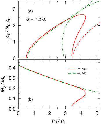
Figure 8: The tensor density normalized by the normal nuclear matter density (a) and the dynamical quark mass (b) with PM1 and $G_{T}=-G_{s}$. The dot-dashed and solid lines represent the results with and without the vacuum contribution (VC), respectively. In the upper panel, the dotted and -dashed lines indicate the tensor density with and without VC in the chiral-restored phases, respectively.

In Fig. 8 we show the tensor density normalized by normal nuclear matter density $\rho_{T}/(N_{c}\rho_{0})$ (a) and the dynamical quark mass $M_{q}$ with PM1 and $G_{T}=-1.2G_{s}$. The solid and dot-dashed lines represent the results without and with the vacuum contribution, respectively.

In the density region, $\rho_{B}\lesssim\rho_{c}$. the results with the vacuum contribution are almost the same as those without the vacuum contribution. In the density region, $\rho_{B}\gtrsim\rho_{c}$, however, the SP ratio is larger than that without the vacuum contribution, and the SP-I phase survives when the vacuum contribution is included. The vacuum polarization has a role to keep the quark mass finite in the SP phase in high density region.

These large vacuum contributions is considered to come from the second term of Eq. (46), which is proportional to $\ln(\Lambda^{2}/M_{q}^{2})$, and becomes larger as the quark dynamical mass decrease. This contribution cannot be removed by a usual renormalization process because a related counter term must be proportional to $M_{q}^{2}U_{T}^{2}$, which becomes smaller with the decrease of $M_{q}$.

References

- (1) For a review, G. Chanmugam, Annu. Rev. Astron. Astrophys. 30 (1992) 143.
-
(2)
P.M. Woods and C. Thompson, Soft gamma ray
repeaters and anomalous X-ray pulsars:magfnetar candidates,
Compact stellar X-ray sources, 2006, 547.
A.K. Harding and D. Lai, Rep. Prog. Phys. 69, 2631 (2006). - (3) P. Braun-Munzinger and J. Stachel, Nature 448, 302 (2007).
-
(4)
For recent reviews,
F. Weber, Prog. in Part. and Nucl. Phys. 54, 193 (2005).
D. Page and S. Reddy, Ann. Rev. of Nucl. and Part. Sci. 56, 327 (2006).
J.M. Lattimer and M. Prakash, Phys. Rep. 442, 109 (2007). -
(5)
T. Schaefer, arXiv:hep-ph/0509068.
P. Braun-Munzinger and J. Wambach, Rev. Mod. Phys, 81, 1031 (2009). - (6) For a recent review, M.G. Alford, A. Schmitt, K. Rajagopal, T. Schaefer, Rev. Mod. Phys, 80, 1455 (2008).
-
(7)
T. Tatsumi, Phys. lett. B489, 280 (2000);
T. Tatsumi, E. Nakano and K. Nawa, Dark Matter, p.39 (Nova Science Pub., New York, 2006). - (8) F. Bloch, Z. Phys. 57 (1929) 545;
-
(9)
C. Herring, Exchange Interactions among Itinerant
Electrons: Magnetism IV (Academic press, New
York, 1966)
K. Yoshida, Theory of magnetism (Springer, Berlin, 1998). - (10) T. Moriya, Spin Fluctuations in Itinerant Electron Magnetism (Springer, 1985)
- (11) T. Maruyama and T. Tatsumi, Nucl. Phys. A693 (2001) 710.
- (12) T. Maruyama, E. Nakano and T. Tatsumi, Horizons in World Physics. Vol.276, Chapt. 7 Nova Science (2011)
- (13) E. Nakano and T. Tatsumi, Phys. Rev. D71, 114006 (2005).
- (14) E. Nakano, T. Maruyama and T. Tatsumi, Phys. Rev. D68 (2003) 105001.
- (15) R. Yoshiike and T. Tatsumi, Phys. Rev. D92, 116009 (2015).
- (16) S. Maedan, Prog. Theor. Phys. 118, 729 (2007).
- (17) Y. Tsue, J. de. Providencia, C. Providencia and M. Yamamura Prog. Theor. Phys. (2012).
- (18) K. Tsushima, T. Maruyama and A. Faessler, Nucl. Phys. A535, 497 (1991).
- (19) T. Maruyama, K. Tsushima and A. Faessler, Nucl. Phys. A537, 497 (1992).
- (20) J. Schwinger, Phys. Rev. 82, 664 (1951).
- (21) G.S. Bali, F. Bruckmann, M. Constantinou, M. Costa, G. Endrodi, S.D. Katz, H. Panagopoulos, A. Schaefer, Phys. Rev. D86, 094512 (2012).
- (22) C. Bonati, M.D’Elia, M. Mariti, F. Negro and F. Sanfilippo Phys. Rev. D 89, 054506 (2014).