BL Lacertae: X-ray spectral evolution and a black-hole mass estimate

Abstract

We present an analysis of the spectral properties observed in X-rays from active galactic nucleus BL Lacertae using RXTE, Suzaku, ASCA, BeppoSAX, and Swift observations. The total time covered by these observations is approximately 20 years. We show strong observational evidence that this source undergoes X-ray spectral transitions from the low hard state (LHS) through the intermediate state (IS) to the high soft state (HSS) during these observations. During the RXTE observations (1997 – 2001, 180 ks, for a total 145 datasets), the source was approximately $\sim 75$%, $\sim 20$% and only $\sim 5$% of the time in the IS, LHS, and HSS, respectively. We also used $Swift$ observations (470 datasets, for a total 800 ks), which occurred during 12 years (2005 – 2016), the broadband (0.3 – 200 keV) data of $Beppo$SAX (1997 – 2000, 160 ks), and the low X-ray energy (0.3 – 10 keV) data of $ASCA$ (1995 – 1999, 160 ks). Two observations of $Suzaku$ (2006, 2013; 50 ks) in combinations with long-term $RXTE$ and $Swift$ data-sets fortunately allow us to describe all spectral states of BL Lac. The spectra of BL Lac are well fitted by the so-called bulk motion Comptonization (BMC) model for all spectral states. We have established the photon index saturation level, $\Gamma_{sat}$=2.2$\pm$0.1, in the $\Gamma$ versus mass accretion rate ($\dot{M}$) correlation. This $\Gamma-\dot{M}$ correlation allows us to estimate the black-hole (BH) mass in BL Lac to be $M_{BH}\sim 3\times 10^{7}M_{\odot}$ for a distance of 300 Mpc. For the BH mass estimate, we use the scaling method taking stellar-mass Galactic BHs 4U 1543–47 and GX 339–4 as reference sources. The $\Gamma-\dot{M}$ correlation revealed in BL Lac is similar to those in a number of stellar-mass Galactic BHs and two recently studied intermediate-mass extragalactic BHs. It clearly shows the correlation along with the very extended $\Gamma$ saturation at $\sim 2.2$. This is robust observational evidence for the presence of a BH in BL Lac. We also reveal that the seed (disk) photon temperatures are relatively low, of order of 100 eV, which are consistent with a high BH mass in BL Lac. It is worthwhile to emphasize that we found particular events when X-ray emission anti-correlates with radio emission. This effect indicates that mass accretion rate (and thus X-ray radiation) is higher when the mass outflow is lower.

1 Introduction

BL Lacertae (BL Lac), B2200+420 is a highly variable active galactic nucleus (AGN), which was discovered approximately a century ago by Cuno Hoffmeister  [see Hoffmeister (1929)]. This source was initially thought to be simply an irregular variable star in the Milky Way galaxy and for this reason was given a variable star notation. Later, the radio counterpart was identified for this “star” by John Schmitt at the David Dunlap Observatory [Schmitt (1968)]. When Oke and Gunn (1974) measured the redshift of BL Lac ($z=0.069$) it became clear that this object is located at a distance of 900 million light years (or $\sim$ 300 Mpc). BL Lac is the eponym for BL Lacertae objects. This class is distinguished by optical spectra where broad emission lines are absent. Note, the broad emission lines are usually characteristics of quasars. Nonetheless,BL Lac sometimes displays weak emission lines. For this reason, BL Lacs are classified based on overall spectrum. Specifically, the BL Lac objects with a low-energy peak located in the UV or X-rays and usually found during X-ray surveys were labeled as “high-energy peaked BL Lacs” or HBLs (see Giommi, Ansari, & Micol 1995; Madejski et al. 1999). While those with the lower-energy peak in the infra-red (IR) range were defined as “low-energy peaked BL Lacs” or LBLs.

To understand blazar variability we should study wide band spectra during major flaring episodes and BL Lac has been a target of many such multi-wavelength campaigns (see for example, Ravasio et al. 2003).

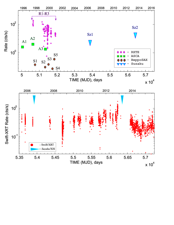
Figure 1: Top: The time distribution of $ASCA$ (green squares, “A”-marks), $RXTE$ (pink diamonds, “R”-marks), $Beppo$SAX (brown stars, “S”-marks), and $Suzaku$ (blue triangles, “Sz”-marks) observations (see Tables 1 – 4). Bottom: The $Swift$/XRT light curve of BL Lac in the 0.3$-$10 keV range during 2005 – 2016. Red points mark the source signal (with 2-$\sigma$ detection level) and blue arrows show the MJD of $Suzaku$. Note, that rate-axis is related to RTXE/PCA count rate which are not comparable with other instruments (ASCA, BeppoSAX and Suzaku). For clarity, the error bars are omitted.

BL Lac is well known for its prominent variability in a wide energy range, particularly, its variability in optical (Larionov et al., 2010; Gaur et al., 2015) and radio (Wehrle et al., 2016). Raiteri et al. (2009) showed the broadband observations from radio to X-rays of BL Lac, which were taken during the 2007 – 2008 Whole Earth Blazar Telescope (WEBT) campaign. They fitted the spectra by an inhomogeneous, rotating helical jet model, which includes synchrotron self-Compton (SSC) emission from a helical jet plus a thermal component from the accretion disk (see also Villata & Raiteri 1999; Ostorero et al. 2004; Raiteri et al. 2003). Larionov et al. (2010) studied the behavior of BL Lac optical flux and color variability and suggested the variability to be mostly caused by changes of the jet. Raiteri et al. (2010) investigated the broad band emission and timing properties of BL Lac during the 2008 – 2009 period and argued for a jet geometry model where changes in the viewing angle of the jet emission regions played an important role in the source’s multiwavelength behavior. Moreover, Raiteri et al. (2013) collected an extensive optical sampling using the GLAST-AGILE Support Program of the WEBT for the BL Lac outburst period during 2008 – 2011 and tested cross-correlations between the optical-$\gamma$-ray and X-ray-mm bands.

BL Lac has been observed by many missions in the X-ray energy band and surveys were conducted using satellites HEAO–1, Einstein, Ginga, ROSAT, ASCA, BeppoSAX, RXTE, and Swift during a 20-year period. Thereafter, the total number of observations and total exposure times of the RXTE and Swift observations (and these two datasets give the most extensive time coverage, the latter covering 2005-2016) and a further three missions covered only a limited number (from two to five) of epochs but with the largest effective area (i.e., best spectral signal-to-noise ratio (SNR) spectra). In the earliest data, Bregman et al. (1990), for example, using the Einstein observations found the best-fit values of $\Gamma$ to be approximately 1.7, on average, while Urry et al. (1996), using $ROSAT$ data, estimated $\Gamma$ to be 1.95$\pm$0.45. Using $GINGA$ observations Kawai et al. (1991) found $\Gamma\sim$ 1.7 – 2.2.

X-ray variability of BL Lac is less well studied in terms of spectral state transition, which is widely investigated in Galactic sources (see e.g., Shaposhnikov & Titarchuk 2009, hereafter ST09). Raiteri et al. (2010) (see Figure 9 therein), constructed spectral energy distributions (SEDs) of BL Lac corresponding to two epochs, when the source had different brightness levels: 2008 (May combined with August) and 1997 (July) based on contemporaneous data from $Swift$ (UV and X-ray), GASP-WEBT (optical and radio) and $Fermi$ ($\gamma$-ray data, Abdo et al. 2010). These SEDs have two strong peaks which are usually associated with the synchrotron and SSC components and they vary in amplitude, spectral shape and peak frequencies. In this paper we concentrate our efforts on studying X-ray variability for BL Lac in the energy range from 0.3 to 150 keV.

It is usually believed that BL Lac contains a supermassive black hole (SMBH) but there is no direct estimate of the value of its BH mass. Magorrian et al. (1998) and Bentz et al. (2009), constructing dynamical models, established correlations between the luminosity of the bulge of the host galaxy and a BH mass, and Ferrarese & Merritt (2000); G$\ddot{u}$ltekin et al. (2009) found a correlation between the velocity dispersion and a BH mass. Moreover, Kaspi et al. (2000), Vestergaard (2002), and Decarli et al. (2010) established the correlation between the luminosity of the continuum at selected frequencies and the size of the Broad Line Region (BLR). They suggested using this correlation to estimate BH mass. In particular, for cases of very powerful blazars, where their IR-optical-UV continuum is dominated by a thermal component, these authors suggested that the thermal component is related to the accretion disk (Ghisellini et al. 2011). Thus, modeling of this radiation using the standard Shakura-Sunyaev disk allows one to estimate a black hole mass as well as an accretion rate.

More details of the methods of BH mass estimates in AGNs can also be revealed from studies based on, for example, reverberation mapping, kinematics in the bulge of the host galaxy of AGN (Blandford & McKee (1982); Peterson (1993), (2014); Peterson et al. (2014); Ferrarese & Merritt (2000); Ryle 2008; G$\ddot{u}$ltekin et al. (2009)), and break frequency scales (see Ryle (2008)). A high BH mass value of its central source in BL Lac actually can give high luminosity along with variability of its emission in all energy bands. For a BH mass estimate in BL Lac, Liang & Liu (2003) used lower timescales of variability, although these estimates are not a robust indicator of a BH mass. Nevertheless, the authors relate them with the photon light-crossing time. Mass determination using this particular method gives a black hole mass, $M_{BH}\sim 3\times 10^{6}$ M_⊙ for BL Lac which differs from that determined using emission of the fundamental plane technique (see Woo & Urry 2002). Using this method, Woo & Urry found that $M_{BH}=1.7\times 10^{8}$ M_⊙ for BL Lac.

Therefore, it is desirable to have an independent BH identification for its central object as well as the BH mass determination by an alternative to the abovementioned methods, based on luminosity estimates only. A method of BH mass determination was developed by Shaposhnikov & Titarchuk (2009), hereafter ST09, using a correlation scaling between X-ray spectral and timing (or mass accretion rate); properties observed for many Galactic BH binaries during their spectral state transitions.

We apply the ST09 method to RXTE, BeppoSAX, ASCA, Suzaku, and Swift/XRT data of BL Lac. Whether or not the observed spectral variability of BL Lac can be explained in terms of spectral state transition remains to be seen. We fitted the X-ray data applying the bulk motion Comptonization (BMC) model along with photoelectric absorption. The parameters of the BMC model are the seed photon temperature $T_{s}$, the energy index of the Comptonization spectrum $\alpha$ ($\alpha=\Gamma-1$), and the illumination parameter $\log(A)$ related to the Comptonized (illumination) fraction $f=A/(1+A)$. This model uses a convolution of a seed blackbody with an upscattering Green’s function, presented in the framework of the BMC as a broken power law whose left and right wings have indices $\alpha+3$ and $\alpha$, respectively (we refer to the description of the BMC Comptonization Green’s function in Titarchuk & Zannias (1998) (TZ98) and suggest comparison with Sunyaev & Titarchuk (1980)).

Previously, many properties of BL Lac were analyzed using Swift/XRT observations. In particular, Raiteri et al. (2010) analyzed the Swift (2008 – 2009) observations and later Raiteri et al. (2013) investigated the Swift observations made from 2009 to 2012 (see the light curve in Figure 1), using fits of their X-ray spectra with a simple absorbed power law model. They found that in the X-ray spectra of BL Lac, the values of $\Gamma$ are scattered between 1.32 (hard spectrum) and 2.37 (soft spectrum) without any correlation with the flux.

ASCA observed BL Lac in 1995 detecting the photon index, $\Gamma$ $\sim 1.94$ (Madejski et al. 1999; Sambruna et al. 1999). RXTE found a harder spectrum with $\Gamma$ in the range 1.4 – 1.6 over a time span of seven days (Madejski et al. 1999). A fit of simultaneous ASCA and RXTE data shows the existence of a very steep and varying soft component for the photon energies $E<$ 1 keV. Photo index $\Gamma$ was in the range 3 – 5, in addition to the hard power law component with $\Gamma$ in the range 1.2 – 1.4. Two rapid flares with time scales of 2 – 3 hours were detected by ASCA in the soft part of the spectrum (Tanihata et al. 2000). In November 1997, BL Lac was observed using the $Beppo$SAX, see Padovani et al. (2001), who estimated $\Gamma$ in the interval of 1.89$\pm$0.12 .

In this paper we present an analysis of available Swift, Suzaku, BeppoSAX, ASCA and RXTE observations of BL Lac in order to re-examine previous conclusions on a BH as well as to find further indications to a supermassive BH in BL Lac. In §2 we show the list of observations used in our data analysis while in §3 we provide details of the X-ray spectral analysis. We discuss an evolution of the X-ray spectral properties during the high-low state transitions and demonstrate the results of the scaling analysis in order to estimate a BH mass of BL Lac in §4. We make our conclusions on the results in §5.

2 Observations and data reduction

We examined X-ray data of BL Lac using a number of instruments with various spectral capabilities covering different energy ranges. BeppoSAX and RXTE cover very wide energy ranges from 0.3 to 200 keV and from 3 keV to 100 keV, respectively. In Sect. 2.1 we present our analysis of the RXTE archival data from 1997 to 2001 (for our sample of 145 observations; approximately 180 ks). We also investigate the BeppoSAX archival data taken around the time interval of the $RXTE$ observations (see Sect. 2.2).

In the upper panel of Figure 1 we show the time distribution of $RXTE$ and $Beppo$SAX indicated by $pink$ diamonds with “$R$”-marks and $brown$ stars with “$S$”-marks, respectively. It is worth noting that the count rates of individual satellites are not comparable between each other. BeppoSAX observations are not so numerous (only five observations) while they cover all spectral states of BL Lac with high energy sensitivity and long time exposure (for a total of 160 ks).

Along with these high-energy observations we also investigate spectral evolution of BL Lac during long-term observations (2005 – 2016) by the $Swift$ X-ray Telescope (XRT; Burrows et al. 2005) in lower (0.3 – 10 keV) energy band (see details in Sect. 2.5). $Swift$ data contain over 470 detections of BL Lac with a total exposure of 800 ks over a 12 year interval (see bottom panel of Fig. 1). We also use for our analysis three observations by $ASCA$ with total exposure of 160 ks (1995 – 1999; see Sect. 2.3), and two detections by $Suzaku$ with an exposure time of approximately 50 ks (2006, 2013; see Sect. 2.4). The MJDs for two $Suzaku$ observations of BL Lac are indicated by blue arrows in the light curve of BL Lac obtained by $Swift$ and shown in the bottom panel of Figure 1. Note, $Suzaku$ points are present in the upper panel to compare with $RXTE$, $ASCA,$ and $Beppo$SAX observations.

All these datasets are spread over twenty years (see Figure 1), sometimes randomly and sometimes covering common intervals. $Suzaku$ provides much better photon statistics than $Swift$ due to the long $Suzaku$ exposures. The total list of BL Lac observations used in our analysis is given in Tables 1$-$5. We applied the nominal position of BL Lac ($\alpha=22^{h}02^{m}43^{s}.3$, $\delta=+42^{\circ}16{\tt{}^{\prime}}39{\tt{}^{\prime\prime}}$, J2000.0 (see, e.g., Ghisellini et al., 2011).

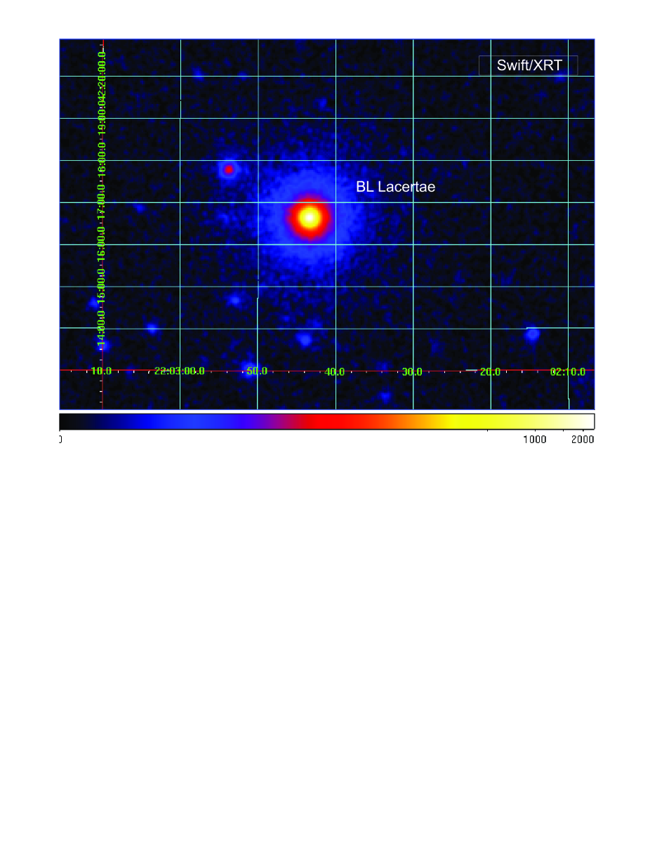
Figure 2: The $Swift$/XRT (0.3 – 10 keV) image of the BL Lac field taken during 2005 – 2016 (800 ks) centered on the nominal position of BL Lac ($\alpha=22^{h}02^{m}43^{s}.3$, $\delta=+42^{\circ}16{\tt{}^{\prime}}39{\tt{}^{\prime\prime}}$, J2000.0). The field is approximately $9^{\prime}\times 15^{\prime}$.

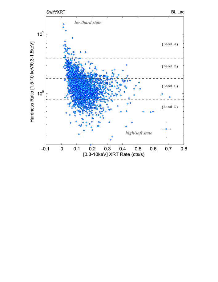
Figure 3: Hardness-intensity diagram for BL Lac using Swift observations (2005 – 2016) during spectral evolution from the low/hard state to the high/soft states. In the vertical axis, the hardness ratio (HR) is a ratio of the source counts in the two energy bands: the hard (1.5 – 10 keV) and soft (0.3 – 1.5 keV). The HR decreases with a source brightness in the 0.3 – 10 keV range (horizontal axis). For clarity, we plot only one point with error bars (in the bottom right corner) to demonstrate typical uncertainties for the count rate and HR.

We extracted all of these data from the HEASARC archives and found that they encompassed a wide range of X-ray luminosities. The well-exposed ASCA, BeppoSAX, and Suzaku data are affected by the low-energy photoelectric absorption, which is presumably not related to the source. The fitting was carried out using the standard XSPEC astrophysical fitting package.

2.1 RXTE

For our analysis, we used 145 RXTE observations taken between July 1997 and January 2001 related to different spectral states of the source. Standard tasks of the LHEASOFT/FTOOLS 5.3 software package were applied for data processing. For spectral analysis we used PCA Standard 2 mode data, collected in the 3 – 23 keV energy range, using PCA response calibration (ftool pcarmf v11.7). The standard dead time correction procedures were applied to the data. In order to construct broad-band spectra, the data from HEXTE detectors were also used. The spectral analysis of the data in the 19 – 150 keV energy range should also be implemented in order to account for the uncertainties in the HEXTE response and background determination. We subtracted the background corrected in off-source observations. The data of BL Lac are available through the GSFC public archive (http://heasarc.gsfc.nasa.gov). Systematic error of 0.5% has been applied to the derived spectral parameters of RXTE spectra. In Table 1 we list the groups of RXTE observations tracing the source evolution during different states.

2.2 BeppoSAX

We used the BeppoSAX data of BL Lac carried out from 1997 to 2000 and found the source was in different spectral states. In Table 2 we show the summary of the BeppoSAX observations analyzed in this paper. Broad band energy spectra of BL Lac were obtained combining data from three BeppoSAX Narrow Field Instruments (NFIs): the Low Energy Concentrator Spectrometer (LECS) for the 0.3 – 4 keV range (Parmar et al. (1997)), the Medium Energy Concentrator Spectrometer (MECS) for the 1.8 – 10 keV range (Boella et al. (1997)), and the Phoswich Detection System (PDS) for the 15 – 200 keV range (Frontera et al. (1997)). The SAXDAS data analysis package is used for the data processing. We performed a spectral analysis for each of the instruments in a corresponding energy range within which a response matrix is well specified. The spectra were accumulated using an extraction region of 8 and 4 arcmin radius for the LECS and MECS, respectively. The LECS data were renormalized to match the MECS data. Relative normalizations of the NFIs were treated as free parameters in the model fits, except for the MECS normalization that was fixed at unity. The obtained cross-calibration factor was found to be in a standard range for each instrument. Specifically, LECS/MECS re-normalization ratio is 0.72 and PDS/MECS re-normalization ratio is 0.93. While the source was bright and the background was low and stable, we checked its uniform distibution across the detectors. Furthermore, we extracted a light curve from a source-free region far from source and found that the background did not vary for the whole observation. In addition, the spectra were rebinned in accordance with the energy resolution of the instruments using rebinning template files in GRPPHA of XSPEC to obtain better signal to noise ratio for derivation of the model spectral parameters. We applied systematic uncertainties of 1% to the derived spectral parameters of BeppoSAX spectra.

2.3 ASCA

$ASCA$ observed BL Lac on November 22, 1995, on July 18, 1997 and June 28, 1999. Table 3 summarizes the start time, end time, and the MJD interval for each of these observations. For the ASCA description, see Tanaka, Inoue, & Holt (1994). The ASCA data were screened using the ftool ascascreen and the standard screening criteria. The pulse-height data for the source were extracted using spatial regions with a diameter of 3’ (for SISs) and 4’ (for GISs) centered on the nominal position of BL Lac, while the background was extracted from source-free regions of comparable size away from the source. The spectrum data were rebinned to provide at least 20 counts per spectral bin in order to validate using the $\chi^{2}$ statistic. The SIS and GIS data were fitted applying XSPEC in the energy ranges 0.6 – 10 keV and 0.7 – 10 keV respectively, where the spectral responses are well known.

2.4 Suzaku

For the Suzaku data (see Table 4) we used the HEASOFT software package (version 6.13) and calibration database (CALDB) released on February 10, 2012. We applied the unfiltered event files for each of the operational XIS detectors (XIS0, 1 and 3) and following the Suzaku Data Reduction Guide. We obtained cleaned event files by re-running the Suzaku pipeline implementing the latest calibration database (CALDB) available since January 20, 2013, and also apply the associated screening criteria files.

Thus, we obtained the BL Lac spectra from the filtered XIS event data taking a circular region, centered on the source, of radius 6’. Using the BeppoSAX sample, we considered the background region to be in the vicinity of the source extraction region. We obtained the spectra and light curves from the cleaned event files using XSELECT, and we generated responses for each detector utilizing the XISRESP script with a medium resolution. The spectra and response files for the front-illuminated detectors (XIS0, 1 and 3) were combined using the FTOOL ADDASCASPEC, after confirmation of their consistency. Finally, we again grouped the spectra to have a minimum of 20 counts per energy bin.

We carried out spectral fitting applying XSPEC package. The energy ranges at approximately 1.75 and 2.23 keV were not used for spectral fitting because of the known artificial structures in the XIS spectra around the Si and Au edges. Therefore, for spectral fits we took the 0.3 – 10 keV range for the XISs (excluding 1.75 and 2.23 keV points).

2.5 Swift

Since the effective area of the $Swift$/XRT is less than for the $Suzaku$/XIS and $Beppo$SAX detectors in the 0.4 – 10 keV range, detailed spectral modeling is difficult to make using $Swift$ data only. Therefore, we analyzed the XRT data in the framework of the BMC model and used photoelectric absorption determined by $Beppo$SAX spectral analysis.

We used $Swift$ data carried out from 2005 to 2016. In Table 5 we show the summary of the Swift/XRT observations analyzed in this paper. In the presented $Swift$ observations, BL Lac shows global outburst peaked in November 2012 (see Figure 1, bottom panel) as well as moderate variability and low flux level intervals, when the source has been detected at least, at $\sim$ 2-$\sigma$ significance (see, Evans et al. 2009). The $Swift$-XRT data in photon counting (PC) mode (ObsIDs, indicated in the second column of Table 5) were processed using the HEA-SOFT v6.14, the tool XRTPIPELINE v0.12.84, and the calibration files (latest CALDB version is 20150721). The ancillary response files were created using XRTMKARF v0.6.0 and exposure maps generated by XRTEXPOMAP v0.2.7. We fitted the spectrum using the response file SWXPC0TO12S6$\_$20010101v012.RMF. We also applied the online XRT data product generator for independent verification of light curves and spectra (including background and ancillary response files, see Evans et al. 2007, 2009).

3 Results

3.1 Images

We made a visual inspection of the source field of view (FOV) image to get rid of a possible contamination from nearby sources. The Swift/XRT (0.3 – 10 keV) image of BL Lac FOV is shown in Fig. 2. It is evident that while some sources are presented in BL Lac FOV, they are far from BL Lac (seen clearly in the center of the FOV). Thus, we excluded the contamination by other bright point sources within a 10 arcmunute radius circle.

3.2 Hardness-intensity diagrams and light curves

Before we proceed with details of the spectral fitting we study a hardness ratio (HR) as a function of soft counts in the 0.3 – 1.5 keV band using the Swift data. Specifically, we consider the HR as a ratio of the hard counts (in the 1.5 – 10 keV range) and the soft ones. The HR is evaluated by careful calculation of background counting and uses only significant points (with 5-$\sigma$ detection). In Figure 3 we demonstrate the hardness-intensity diagram (HID) and thus, we show that different count-rate observations are associated with different color regimes. Namely, the HR larger values correspond to harder spectra. A Bayesian approach was used to estimate the HR values and their errors [Park et al. (2006)].

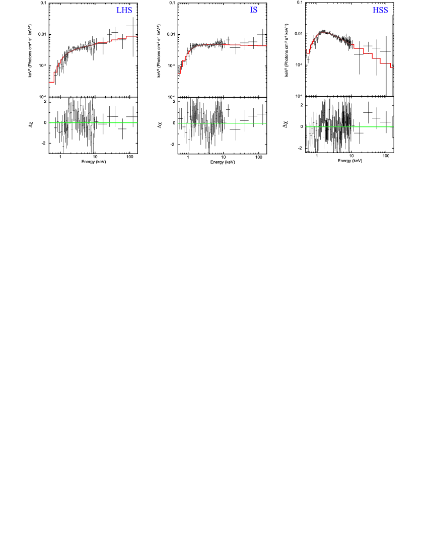
Figure 4: Three representative $EF_{E}$ diagrams for different states of BL Lac. Data are taken from $Beppo$SAX observations S1 (left panel, LHS), S2 (central panel, IS), and S5 (right panel, HSS). The data are shown by black crosses and the spectral model (phabs*BMC) is displayed as a red line.

Figure 3 indicates that the HR monotonically reduces with the total count rate (in the 0.3 – 10 keV energy band). This particular sample is similar to those of most outbursts of Galactic X-ray binary transients (see Belloni et al. 2006; Homan et al. 2001; Shaposhnikov & Titarchuk, 2006; ST09; TS09; Shrader et al. 2010; Mu$\tilde{n}$oz-Darias et al. 2014).

We show the Swift/XRT light curve of BL Lac from 2005 to 2016 for the 0.3 – 10 keV band in Figure 1. Red points mark the source signal. Thus, one can see that BL Lac shows rapid variability on timescales of less than 10 ks, while in 2012 the source showed a higher count level, which could be associated with the global outburst. The maximum of the outburst was at approximately MJD 56250 for a total rise-decay sample of 2.5 years. For most of the Swift observations the source remained in the low or intermediate state and was in the soft state for only 5% of the time. We should point out that individual Swift/XRT observations of BL Lac in PC mode do not have enough counts into make statistically significant spectral fits.

Based on the hardness-intensity diagram for BL Lac (see Fig. 3) we also made the state identification using the hardness ratio. This plot indicates a continuous distribution of the HR with source intensity from high hardness ratio at lower count-rate to low hardness ratio at higher count events. Furthermore, the hardness$-$intensity diagram shows a smooth track. Therefore, we grouped the $Swift$ spectra into four bands according to count rates: very high (”A”, HR¿4), high (”B”, $1.9<HR<4$), intermediate (”C”, $0.8<HR<1.9$), and low (”D”, $HR<0.8$) count rates to resolve this problem. In addition, all groups of the Swift spectra were binned to a minimum of 20 counts per bin in order to use $\chi^{2}$-statistics for our spectral fitting. Thus, we combined the spectra in each related band, regrouping them with the task grppha and then we fitted them using the 0.3 – 10 keV range.

3.3 X-Ray spectral analysis

Various spectral models were used in order to test them for all available data sets for BL Lac. We wanted to establish the low/hard and high/soft state evolution using spectral modeling. We investigate the Suzaku, $Beppo$SAX, ASCA, RXTE, and combined Swift spectra to check the following spectral models: powerlaw, blackbody, BMC and their possible combinations modified by an absorption model.

Since BL Lac is located relatively close to the Galactic plane ($b=-10.43$ deg), it is necessary to take into account the possible contribution from the Galactic molecular gas in addition to that associated with neutral hydrogen 21 cm values. Furthermore, the source is located behind a molecular cloud from which CO emission and absorption have been detected (Bania, Marscher, & Barvainis 1991; Marscher, Bania, & Wang 1991; Lucas & Liszt 1993). The equivalent atomic hydrogen column density of the CO cloud is $N_{H}\approx 1.6\times 10^{21}$ cm^-2 (Lucas & Liszt 1993). Thus, the total absorbing column density in the direction of BL Lac consists of two components, that associated with neutral hydrogen, $1.8\times 10^{21}$ cm^-2 inferred from the 21 cm measurements of Dickey et al. (1983) and the molecular component, yielding the total column $\sim 4.6\times 10^{21}$ cm^-2. For BeppoSAX data we found the $N_{H}$ value in a wide range (2.1 – 7.5)$\times 10^{21}$ cm^-2 depending on an applied model and the source spectral state (see Table 6), which is in agreement with the total column value from the aforementioned radio measurements. The residuals shown in Figure 4 indicate that the observed spectra are in good agreement with the $BMC$ model. Thus, we fitted all observed spectra using a $Beppo$SAX neutral column range. We note, that the $N_{H}$ value of $2.6\times 10^{21}$ cm^-2 is mostly suitable for the rest (long-term $RXTE$ and $Swift$ observations), which is also obtained as the best-fit column $N_{H}$ for $ASCA$ observations (see also Madejski et al, 1999; Sambruna et al., 1999).

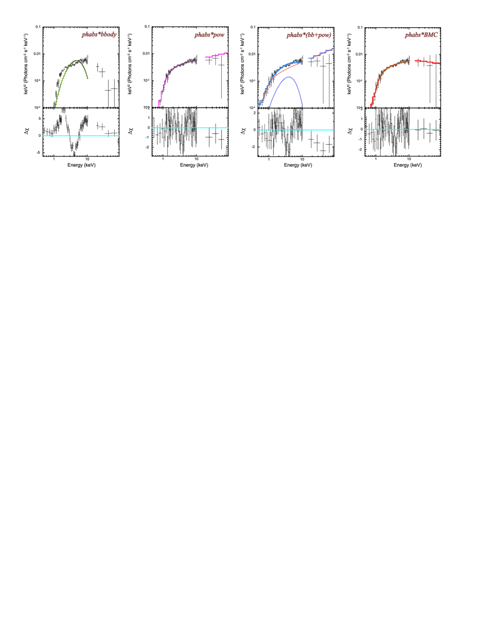
Figure 5: The best-fit spectra of BL Lac observed with $Beppo$SAX during the soft state in 1999 transition (dataset “S3”) in $E*F(E)$ units for the model fits (from left to right): phabs*bbody (green line, $\chi^{2}_{red}=1.3$ for 79 dof), phabs*powerlaw (purple line, $\chi^{2}_{red}=2.31$ for 79 dof), phabs*(bbody+powerlaw) (light-blue line, $\chi^{2}_{red}=1.78$ for 77 dof) and phabs*BMC (red line, $\chi^{2}_{red}=1.17$ for 77 dof). The data are shown by black crosses. For an additive model, phabs*(bbody+powerlaw), the model components are presented by dashed blue and red lines for Blackbody and Powerlaw, respectively (see details in Table 6).

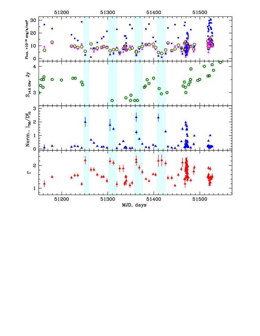
Figure 6: From Top to Bottom: Evolutions of the model flux in the 3 – 10 keV, 10 – 20 keV, and 20 – 50 keV ranges (yellow,crimson, and blue points, respectively) using $RXTE$/PCA, the flux density $S_{14.5GHz}$ at 14.5 GHz (UMRAO), the BMC normalization and $\Gamma$ during the 1999 flare transition (R3, R5). Blue vertical strips indicate the phases, when X-ray flux ($E>$ 3 keV) anticorrelates with $\Gamma$ and the normalization $N_{BMC}$.

3.3.1 Details of spectral modeling

We obtained that the absorbed single power-law (phabs*power-law) model fits well the low and high states data only for “S1” spectrum, $\chi^{2}_{red}$=1.15 (80 d.o.f.), and “S5” spectrum, $\chi^{2}_{red}$=1.05 (116 d.o.f.) (see Table 2 for the notations of observations, S1-S5, and Table 6 for the details of the spectral fits). We establish that the power-law model gives unacceptable fit quality, $\chi^{2}$ for all “S2 – S4” observed spectra of $Beppo$SAX , in which a simple power-law model produces a hard excess. These significant positive residuals at high energies, greater than 10 keV, suggest the presence of additional emission components in the spectrum. Moreover, the thermal model (Blackbody) gives us even worse fits. As a result we tried to check a sum of blackbody and power-law models. In this case the model parameters are $N_{H}=(2.7-4.7)\times 10^{21}$ cm^-2; $kT_{bb}=0.37-1.02$ keV and $\Gamma=1.46-2.4$ (see more details in Table 6). The best fits of the BeppoSAX spectra have been found using the Bulk Motion Comptonization model (BMC XSPEC model, Titarchuk et al. (1997)), for which $\Gamma$ ranges from 1.8 to 2.2 for all observations (see Table 6 and Figures 4-5). Figure 5 shows the best-fit spectrum of BL Lac observed by $Beppo$SAX during the soft state in the 1999 transition (dataset “S3”) presented in $E*F(E)$ units using different frame models (from left to right): phabs*bbody (green line, $\chi^{2}_{red}=1.3$ for 79 dof), phabs*powerlaw (purple line, $\chi^{2}_{red}=2.31$ for 79 dof), phabs*(bbody+powerlaw) (light-blue line, $\chi^{2}_{red}=1.78$ for 77 dof), and phabs*BMC (red line, $\chi^{2}_{red}=1.17$ for 77 dof). The data are shown by black crosses. In particular, for an additive model phabs*(bbody+powerlaw), the blackbody and powerlaw components are presented by blue and red dashed lines, respectively (see details in Table 6). We should emphasize that all $Beppo$SAX best-fit results are found using the same model (BMC) for the high and low states.

Our $Beppo$SAX data analysis provides strong arguments in favor of the BMC model to describe X-ray spectral evolution of BL Lac throughout all spectral states. Thus, we decided to analyze all available spectral data of BL Lac using the BMC model. We provide a short description of the BMC model in the Introduction. As one can see, the BMC has the main parameters, $\alpha$, $A$, the seed blackbody temperature $T_{s}$ and the BB normalization, which is proportional to the seed blackbody luminosity and inversely proportional to $d^{2}$ where d is the distance to the source (see also TS16). We also apply a multiplicative $phabs$ component characterized by an equivalent hydrogen column, $N_{H}$ in order to take into account an absorption by neutral material.

Thus, using the same model, we carried out the spectral analysis of $ASCA$, $Suzaku$, $Swift/XRT$ and $RXTE$ observations and found that BL Lac was in the three spectral states (LHS, IS, HSS). The best-fit $\Gamma$-values are presented in Tables 7 and 8 and in Figures 4-8. An evolution between the low state and high state is accompanied by a monotonic increase of the normalization parameter $N_{BMC}$ from 0.5 to 70$\times L_{34}/d_{10}^{2}$ erg/s/kpc² and by an increase of $\Gamma$ from 1.1 to 2.2 (see Figure 8). Here, we use $L_{34}$ and $d_{10}$ as notations for soft photon luminosity in units of $10^{34}$ erg s^-1 and the distance to the source in units of 10 kpc, respectively (see also Table 6).

Note, that during the RXTE observations (from 1997 to 2001), the source was in the IS, LHS, and HSS, for approximately 75%, 20%, and 5% of the time, respectively.

In Figure 4 we demonstrate three representative $EF_{E}$ spectral diagrams for different states of BL Lac. Data are taken from $Beppo$SAX observations 5004600400 (left panel, S1 set, LHS), 5088100100 (central panel, S2 set, IS), and 511650011 (right panel, S5 set, HSS). The data are represented by black crosses and the spectral model is displayed by a red line. In the bottom panels we show the corresponding $\Delta\chi$ versus photon energy (in keV).

The best-fit model parameters for the HSS (right panel, S5) are $\Gamma$=2.2$\pm$0.2, $N_{BMC}$=(3.08$\pm$0.06) $L_{34}/d^{2}_{10}$ erg/s/kpc², $kT_{s}=50\pm 10$ eV and $\log(A)$=0.35$\pm$0.07 [$\chi^{2}_{red}$=1.08 for 114 d.o.f], while the those parameters for the IS (central panel, S2) are $\Gamma$=2.07$\pm$0.09, $N_{BMC}$=(0.6$\pm$0.2) $L_{34}/d^{2}_{10}$ erg/s/kpc², $kT_{s}$=108$\pm$9 eV and $\log(A)$=0.24$\pm$0.09 [$\chi^{2}_{red}$=0.87 for 80 d.o.f]; and those for the LHS (left panel, S1) are $\Gamma$=1.8$\pm$0.1, $N_{BMC}$=(0.36$\pm$0.09) $L_{34}/d^{2}_{10}$ erg/s/kpc², $kT_{s}$=73$\pm$5 eV and $\log(A)$=-0.32$\pm$0.04 [$\chi^{2}_{ref}$=1.06 for 78 d.o.f].

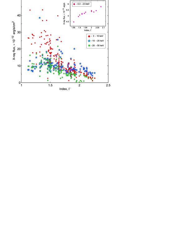
Figure 7: Hard X-ray flux ($E>$ 3 keV) versus the photon index for the 3 – 10 keV (red circle), 10 – 20 keV (blue stars) and 20 – 50 keV (green squares) using the RXTE observations of BL Lac (1997 – 2001). Soft X-ray flux [0.3 – 2.5 keV] versus the photon index is plotted in the incorporated panel (top right) using $Suzaku$ and $Swift$ observations (see also Tables 4-5).

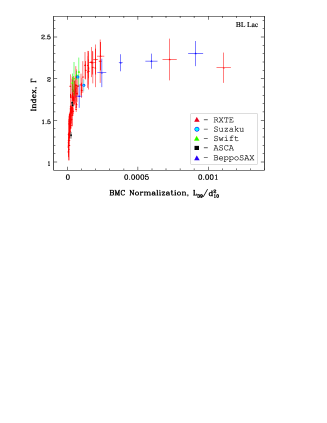
Figure 8: Correlations of $\Gamma$ versus the BMC normalization, $N_{BMC}$ (proportional to mass accretion rate) in units of $L_{39}/d^{2}_{10}$.

Thus, we obtain that the seed temperatures, $kT_{s}$ of the $BMC$ model vary from 50 to 110 eV. We also find that the parameter $\log(A)$ of the $BMC$ component varies in a wide range between -0.86 and 0.24, (the illumination fraction $f=A/(1+A)$) and thus, $f$ undergoes drastic changes during an outburst phase for all observations.

We should point out the fact that all of the HSS, IS and LHS spectra are characterized by a strong soft blackbody (BB) component at low energies and a power law extending up to 100 keV, which is in good agreement with the Comptonization of soft photons (see, e.g., Sunyaev & Titarchuk (1980) and TLM98) for an X-ray emission origin.

For the BeppoSAX observations (see Tables 2, 6) we find that the spectral index $\alpha$ monotonically increases from 0.8 to 1.2 (or $\Gamma$ from 1.8 to 2.2), when the normalization of $BMC$ component (or mass accretion rate) increases by a factor of 8. We illustrate this index versus mass accretion rate correlation in Figure 8 (see $blue$ triangles).

From Figure 8, it is also seen that $\Gamma,$ as a function of the normalization parameter $N_{BMC}$ , displays a strong saturation part at high values of the normalization $N_{BMC}$ (which is proportional to mass accretion rate). It is interesting that previous spectral analyses of $Swift$ X-ray data for BL Lac (Raiteri et al, 2013) show that the $\Gamma$ values are scattered between 1.32 (hard spectrum) and 2.37 (soft spectrum) without correlation with the flux.

It is worth noting that Wehrle et al. (2016) combined these $Swift$/XRT data in their low, medium, and high states in order to determine whether or not the energy index changed when the source was brighter or fainter. They found that brighter states tended to have harder X-ray spectra. They revealed the same result based on $RXTE$ data in the 2 – 10 keV range. Specifically, they argued that the spectral index tended to flatten when the source was bright, and conversely, became steeper when the source was faint.

However, we should notice that all Wehrle’s spectral studies used a simple power-law model and the brightness was related to the 2 – 10 keV range. Therefore, the power-law index was inspected as a function of relatively hard X-ray brightness (Wehrle et al., 2016). In contrast, in Figure 7 we tested the behavior of $\Gamma$ in the framework of the $BMC$ model and investigated the $\Gamma-Flux$ evolution for different energy bands: the 3 – 10 keV ($red$ circle), 10 – 20 keV ($blue$ stars) and 20 – 50 keV ($green$ squares) using $RXTE$ observations BL Lac (1997 – 2001), as well as the 0.3 – 2.5 keV ($pink$ circles; see incorporated top right panel) using $Swift$ and $Suzaku$ observations. From this Figure one can clearly see that hard X-ray flux ($E>$ 3 keV) decreases with respect to $\Gamma$ (see also Wehrle et al., 2016), while softer X-ray flux ($E<2.5$ keV) increases when $\Gamma$ increases (see the incorporated panel). Thus, we should emphasize that the $\Gamma-Flux$ relation for BL Lac is an energy dependent correlation.

To make the RXTE data analysis we used information obtained using the $Beppo$SAX, $ASCA$ and $Suzaku$ best-fit spectra, which can provide well calibrated spectra at soft energies ($E<$ 3 keV). Because the RXTE/PCA detectors cover energies above 3 keV, for our analysis of the RXTE spectra we fixed a key parameter of the BMC model ($kT_{s}=$ 70 eV) obtained as a mean value of $kT_{s}$ in our analysis of the BeppoSAX spectra.

In Figure 6, from the top to the bottom we demonstrate evolutions of the model flux in the 3 – 10 keV, 10 – 20 keV, and 20 – 50 keV energy ranges (yellow, crimson, and blue points, respectively), the flux density $S_{14.5GHz}$ at the 14.5 GHz (UMRAO, Villata et al., 2009), the BMC normalization, and $\Gamma$ for the 1999 flare transition (R2). Blue vertical strips mark intervals when hard X-ray emission ($E>3$ keV) anticorrelates with $\Gamma$ and the normalization $N_{BMC}$.

The spectral evolution of BL Lac was previously investigated using some of the $Swift$ data (see for example, $Sw1$, $Sw3$ and $Sw4$ in Table 5) by many authors. In particular, Wehrle et al. (2016) analyzed the 2012 – 2013 $Swift$ data (partially, $Sw1$ and $Sw3$) and the long (2005 – 2011) $RXTE$ observations, while Raiteri et al. (2010) studied the $Swift$ observation of BL Lac during the 2008 – 2009 period ($Sw1$, $Sw3$ and $Sw4$). Furthermore, Raiteri et al. (2013) reexamined the $Swift$ observations of BL Lac during the period 2008 – 2012 and compared them with the $RXTE$ observations of BL Lac for the same period.

Wehrle et al. (2016) modeled their $Swift$ data using a single power-law continuum and Galactic absorption for which hydrogen column density $N_{H}=3.4\times 10^{21}$ cm^-2. They described the spectrum of BL Lac for the low, medium, and high source states with different spectral indexes, $\alpha_{X}\sim 0.97$, 0.86, and 0.67 ($\alpha_{X}=\Gamma_{X}-1$), respectively. They concluded that the spectral index decreased when the source made a transition from low to high states. Then, Wehrle et al. (2016) checked this behavior using the $Swift$ data sets in combination with $NuSTAR$ (3 – 70 keV) observations of BL Lac, applying three models: power law [phabs*pow], broken power law [phabs*bknpow], and log-parabolic [phabs*logpar] models. As a result, assuming a power-law model with fixed $N_{H}$, they found acceptable fits with $\Gamma\sim 1.9$, on average. The broken power-law and log-parabolic models improved the fit quality, with $\Gamma\sim 2$, on average. It is interesting that results of these fittings suggested that the observed X-ray spectrum of BL Lac might be steeper at softer photon energies than at harder ones.

Raiteri et al. (2010) tested the $Swift$ data set (2008 – 2009, partly $Sw1$, $Sw3$ and $Sw4$) using their spectral analysis. First they fitted spectra using a single power law with free absorption, and then they fixed the Galactic absorption at $N_{H}=3.4\times 10^{21}$ cm^-2. Due to poor statistics, they applied a double power law model to BL Lac spectra. Although, fits using free absorption gave very variable $N_{H}$, which corresponded to unreal changes of absorption. Therefore, they favored the second model with fixed $N_{H}$ and acceptable $\chi^{2}$. For some spectra, a double power law model with absorption fixed to the Galactic value definitely improved the fit quality. Raiteri et al. (2010) argued that $\Gamma$ ranges from 1.9 to 2.3, indicating that these spectra varied from hard to soft (with the average value $\Gamma\sim 2$). Finally, Raiteri et al. (2013) refitted the BL Lac spectra (around $Sw1$, $Sw3$, $Sw4$ periods) applying an absorbed power law with the same value of $N_{H}$ as that used by Wehrle et al. As a result, they found that the source made a transition from the hard state ($\Gamma$=1.3) to the soft state ($\Gamma$=2.4) without any correlation with the source flux. As one can see, Wehrle’s and Raiteri’s studies did not account for the low-energy excess, particularly in the soft state of the source.

We have also found a similar spectral behavior using our BMC model along with the full set of the $Swift$ observations. In particular, as in the aforementioned Wehrle’s and Raiteri’s et al. papers, we also reveal that BL Lac demonstrates the quasi-constancy of $\Gamma$ during the IS – HSS transition. Furthermore, we find that $\Gamma$ strongly saturates at 2.2 at high values of $N_{bmc}$ (or at high values of the mass accretion rate).

In the LHS, the seed photons with lower $kT_{s}$, related to lower mass accretion rate, are Comptonized more efficiently because the illumination fraction $f$ (or $\log(A)$) is higher. In contrast, in the HSS, these parameters, $kT_{s}$ and $\log(A)$ show an opposing behavior; namely $\log(A)$ is lower for higher $kT_{s}$. This means that a relatively small fraction of the seed photons, whose temperature is higher because of the higher mass accretion rate in the HSS than in the LHS, is Comptonized.

Thus, our spectral model shows very good performance through all data sets. In Tables 7 and 8 we demonstrate a good performance of the BMC model in application to the $ASCA$, $Suzaku$, $Swift$ and $RXTE$ data. The reduced $\chi^{2}_{red}=\chi^{2}/N_{dof}$ (where $N_{dof}$ is the number of degrees of freedom) is less; approximately 1 ($0.72<\chi^{2}_{red}<1.15$) for all observations.

4 Discussion

Before proceeding with an interpretation of the observations, let us briefly summarize them as follows. i) The spectral data of BL Lac are well fitted by the BMC model for all analyzed LHS and HSS spectra (see e.g., Figure 4 and Tables 6, 7 and 8). ii) The Green’s function index of the BMC component $\alpha$ (or $\Gamma$) monotonically rises and saturates with an increase of the BMC normalization (proportional to $\dot{M}$). The photon index saturation level of the BMC component is approximately 2.2 (see Figure 8). iii) Blazar BL Lac undergoes spectral state transitions during X-ray outburst events. The X-ray evolution of BL Lac is characterized by a number of similarities with respect to those in Galactic BHs (GBHs). For example, the X-ray spectral index of BL Lac demonstrates a saturation phase in its soft state in the same manner as that in GBHs. In the soft states of GBHs we do not see their jets and outflow (associated with radio emission, see, e.g., Migliari & Fender 2006).

Below, in Sect. 4.1, we demonstrate some episodes in which radio emission is completely suppressed during the X-ray soft state. Quenching of the radio emission in the soft state of BL Lac is in agreement with that found in GBHs (see e.g., GRS 1915+105 (TS09)). Furthermore, BL Lac is well known by its prominent variability in optical (see Larionov et al., 2010; Gaur et al., 2015) and radio bands (Wehrle et al., 2016). Thus, the correlations between optical and radio emissions are deeply investigated. However, the study of the BL Lac variability in X-rays and its possible correlations (or anti-correlations) between X-ray and radio emissions have only recently been developed . While the X-ray has a relatively narrow energy range (0.3 – 150 keV) in comparison with the broad-band SEDs, its variability points to the broad-band variability of BL Lac. The X-ray part of the spectrum is intermediate between two global peaks: at low energies (optical/IR–UV) and high-energies (up to $\gamma$-rays). Below we investigate the connection between the radio flux density and X-ray flux and we find that it is qualitatively similar to that found in GBHs.

4.1 Connection between radio and X-ray emission in BL Lac

The 230 GHz (1.3 mm) light curve was obtained using the Submillimeter Array (SMA) in Mauna Kea (Hawaii), see Villata et al. (2009). In Figure 6 we present an evolution of the flux density $S_{14.5GHz}$ at 14.5 GHz (UMRAO, Villata et al., 2009, Aller et al. 1985) along with a spectral parameter evolution such as the BMC normalization and $\Gamma$ during the 1999 flare transition set (R2). Blue vertical strips indicate the phases when the radio flux ($S_{14.5GHz}$) anticorrelates with $\Gamma$ and the normalization, $N_{BMC}$. We should point out a clear anti-correlation between the radio flux density and $\Gamma$, similar to that identified in some Galactic microquasars, for example in GRS 1915+105 (see discussion below).

Due to lack of the soft X-ray monitoring, $E<3$ keV. During the RXTE observations we associate soft X-ray evolution with the evolution of $N_{BMC}$ (which is proportional to the seed soft photon flux). We formulate the most important results for BL Lac: (i) The strong radio flare occurs usually on the eve of X-ray flare and (ii) during proper X-ray flare the radio flux density significantly decreases. For example, for the RXTE data (1999, set R3, R5), the MJD intervals of strong $N_{BMC}$ (soft X-ray flare) coincide with low radio flux density $S_{14.5GHz}$ , indicated by blue vertical strips (e.g., centered on MJD 51250, 51305, 51350, 51415, 51475, see Fig. 6). It is interesting that these intervals are accompanied by the increase of $\Gamma$ above $2$. A similar relation between radio (230 GHz) and hard X-ray behavior in BL Lac was also found for the $Swift$ observations from October to- November 2012.

In Figure 9, from the top to the bottom we show evolutions of the 230 GHz/345 GHz (pink/green flux densities (see also Wehrle et al., 2016)); flux in the 1.5 – 10 keV (black points); and flux in the 0.3 – 1.5 keV (red points) as a function of MJD time. From this Figure one can see that the X-ray flare (1.5 – 10 keV, see MJD 56229) is developed at the low level of radio flux density, which can also indicate a possible episode of anticorrelation between the radio and X-ray emissions observed in BL Lac.

This anticorrelation between the radio and X-ray emissions observed in BL Lac suggests a inflow/outflow scenario. Strong radio flux is usually associated with a powerful outflow in the form of jet or outflow (wind). In contrast, the X-ray emission is accompanied by a powerful accretion inflow. Thus, the outflow and inflow effects lead to anticorrelation between corresponding X-ray and radio emissions. During the inflow episode (converging inflow case), an accretion is seen as X-ray emission while radio emission is suppressed. Alternatively, for the outflow event (a divergent flow case), the radio emission is dominant and thus, inflow (accretion) observed in X-rays is suppressed. Therefore, divergent and converging cases of the flow around the central object relate to the corresponding regimes of the radio and X-ray dominances.

Radio emission (at 230 GHz and 345 GHz) is more variable than emission in the X-ray range observed by $Swift$ during the period October – November 2012 (see Fig. 9). This might suggest possible different origins of radio and soft X-rays. Radio emission could be related to jet blobs (knots), while soft X-rays emerge from the inner part of accretion disk.

4.2 Saturation of the index as a signature of a BH

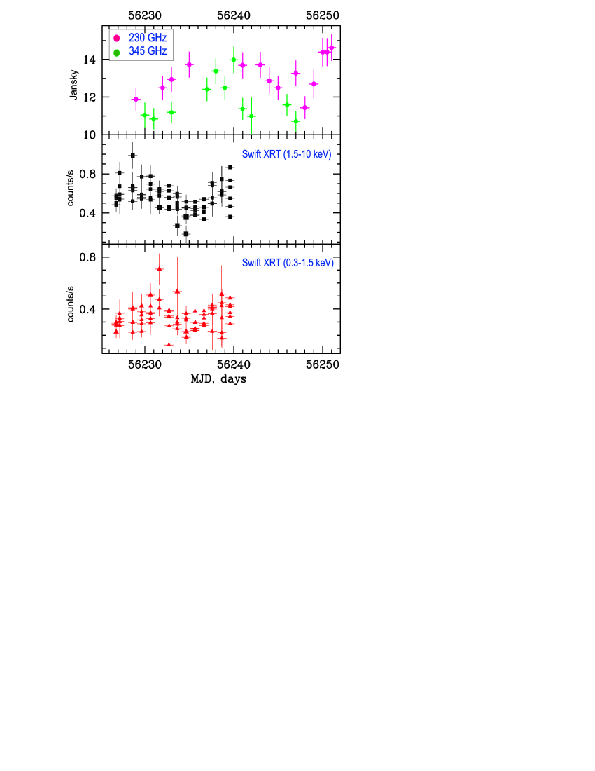
Figure 9: From Top to Bottom: Evolution of the flux density $S_{230GHz}$ (pink) and $S_{345GHz}$ (green points) at 230 GHz and 345 GHz (SMA), the model flux in the 1.5 – 10 keV (black points, Swift XRT), the model flux in the 0.3 – 1.5 keV (blue points, Swift XRT), and X-ray hardness ratio HR.

We establish that $\Gamma$ correlates with the BMC normalization, $N_{BMC}$ (which is proportional to $\dot{M}$) and finally saturates at high values of $\dot{M}$ (see Figure 8). Titarchuk & Zannias (1998) developed the semi-analytical theory of X-ray spectral formation in the converging flow into a BH. They demonstrated that the spectral index of the emergent X-ray spectrum saturated at high values of mass accretion rate (at higher than the Eddingtion one). Later analyzing the data of RXTE for many black hole candidates (BHs) ST09 and Titarchuk & Seifina (2009), Seifina & Titarchuk (2010) and STS14 demonstrated that this index saturation effect was seen in many Galactic BHs (see for example, GRO J1655-40, GX 339-4, H1743-322, 4U 1543-47, Cyg X-1, XTEJ1550-564, GRS 1915+105 ). The levels of the index saturation are at different values which presumably depend on the plasma temperature of the converging flow [see Monte Carlo simulations by Laurent & Titarchuk (1999), (2011)].

For our particular source, BL Lac, we also reveal that $\Gamma$ monotonically increases from 1.2 and then finally saturates at a value of 2.2 (see Figure 8). Using the index-$\dot{M}$ correlation found in BL Lac we can estimate a BH mass in this source using scaling of this correlation with those detected in a number of GBHs (below see the details).

4.3 An estimate of BH mass in BL Lacertae

To estimate the BH mass, $M_{BH}$ , of BL Lac, we chose two galactic sources, 4U 1543–47 and GX 339–4 (see ST09), as the reference sources whose BH masses ($M_{1543}=9.4\pm 1.0$ M_⊙, see Orosz 2003; $M_{339}>6$ M_⊙, see Mu$\tilde{n}$oz-Dariaz et al. 2004) and distances ($d_{1543}=9.1\pm 1.1$ kpc, see Orosz et al., 1998; $d_{339}=7.5\pm 1.6$ kpc, see Hynes et al., 2004) have now been well established (see Table 10). The BH mass in 4U 1543–47 was also estimated applying dynamical methods (Orosz, 2003). For a BH mass estimate of BL Lac we used the BMC normalizations, $N_{BMC}$ of these reference sources.

Thus, we scaled the index versus $N_{BMC}$ correlations for these reference sources with that of the target source BL Lac (see Fig. 10). The value of the index saturation is almost the same, $\Gamma\sim 2.2,$ for all these target and reference sources. We applied the correlations found in these two reference sources to make a comprehensive cross-check of a BH mass estimate for BL Lac.

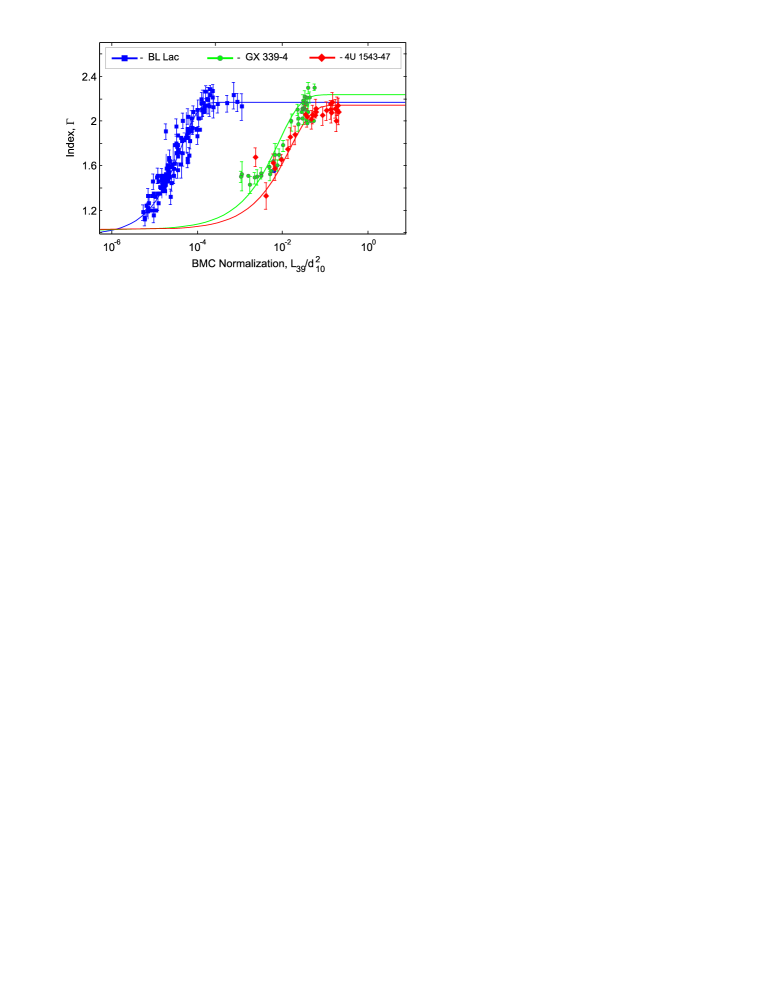
Figure 10: Scaling of $\Gamma$ versus the normalization $N_{BMC}$ for BL Lac (blue squares – target source) using those correlations for the Galactic reference sources, GX 339–4 (green circles) and 4U 1543–47 (red diamonds).

As one can see from Figure 10, the correlations of the target source (BL Lac) and the reference sources have similar shapes and index saturation levels. Hence, it allows us to make a reliable scaling of these correlations with that of BL Lac. The scaling procedure was implemented in a similar way as in ST09, Titarchuk & Seifina 2016a, 2016b, hereafter TS16a and TS16b. We introduce an analytical approximation of the $\Gamma(N_{bmc})$ correlation, fitted by a function

$${\cal F}(x)={\cal A}-({\cal D}\cdot{\cal B})\ln\{\exp[(1.0-(x/x_{tr})^{\beta})/{\cal D}]+1\}$$ (1)

with $x=N_{bmc}$.

Fitting of the observed correlation by this function ${\cal F}(x)$ provides us a set of the best-fit parameters $\cal A$, $\cal B$, $\cal D$, $x_{tr}$, and $\beta$. A more detailed description of these parameters is given in TS16a.

In order to implement this BH mass determination for the target source one should rely on the same shape of the $\Gamma-N_{bmc}$ correlations for the target source and those for the reference sources. To estimate BH mass, $M_{t}$ , of BL Lac (target source), one should slide the reference source correlation along the $N_{bmc}-$axis to that of the target source (see Fig. 10),

$$M_{t}=M_{r}\frac{N_{t}}{N_{r}}\left(\frac{d_{t}}{d_{r}}\right)^{2}f_{G},$$ (2)

where t and r correspond to the target and reference sources, respectively and a geometric factor, $f_{G}=(\cos\theta)_{r}/(\cos\theta)_{t}$; the inclination angles $\theta_{r}$, $\theta_{t}$ and $d_{r}$, $d_{t}$ are distances to the reference and target sources, respectively (see ST09). One can see values of $\theta$ in Table 10 and if some of these $\theta$-values are unavailable then we assume that $f_{G}\sim 1$.

In Figure 10 we demonstrate the $\Gamma-N_{bmc}$ correlation for BL Lac (blue squares) obtained using the $RXTE$, $ASCA$, $Suzaku$, $Swift$ and $Beppo$SAX spectra along with the correlations for the two Galactic reference sources, GX 339–4 (green circles) and 4U 1543–47 (red diamonds). BH masses and distances for each of these target-reference pairs are presented in Table 10.

A BH mass, $M_{t}$ , for BL Lac can be evaluated using the formula (see TS16a)

$$M_{t}=C_{0}{N_{t}}{d_{t}}^{2}f_{G},$$ (3)

where $C_{0}=(1/d_{r}^{2})(M_{r}/N_{r})$ is the scaling coefficient for each of the pairs (target and reference sources), masses $M_{t}$ and $M_{r}$ are in solar units, and $d_{r}$ is the distance to a particular reference source measured in kpc.

We use values of $M_{r}$, $d_{r}$, $d_{t}$, and $\cos(i)$ from Table 10 and then we calculate the lowest limit of the mass, using the best fit value of $N_{t}=(9.6\pm 0.1)\times 10^{-5}$ taking them at the beginning of the index saturation (see Fig. 10) and measuring in units of $L_{39}/d^{2}_{10}$ erg s^-1 kpc^-2 [see Table 9 for values of the parameters of function ${\cal F}(N_{t})$ (see Eq. 1)]. Using $d_{r}$, $M_{r}$, $N_{r}$ (see ST09) we found that $C_{0}\sim 3.5$ and $3.34$ for GX 339–4 and 4U 1543–47, respectively. Finally, we obtain that $M_{bl}\geq 2.7\times 10^{7}~{}M_{\odot}$ ($M_{bl}=M_{t}$) assuming $d_{bl}\sim$300 Mpc  and $f_{G}\sim 1$. To determine the distance to BL Lac (2200+420) we use the formula

$$d_{bl}=z_{bl}c/H_{0},$$ (4)

where the redshift $z_{bl}=0.069$ for BL Lac (2200+420) (see Wright 2006), $c$ is the speed of light and $H_{0}=70.8\pm 1.6$ km s^-1 Mpc^-1 is the Hubble constant. We summarize all these results in Table 10.

It is worth noting that the inclination of BL Lac may be different from those for the reference Galactic sources (e.g., $i\sim 20^{\circ}$ for 4U 1543–47), therefore we take this BH mass estimate for BL Lac as the lowest BH mass value because $M_{bl}$ is a reciprocal function of $\cos(i_{bl})$ (see Eq. 3 taking into account that $f_{G}=(\cos\theta)_{r}/(\cos\theta)_{t}$ there).

The obtained BH mass estimate is in agreement with a “fundamental plane” estimate ($M_{bl}\sim 1.7\times 10^{8}M_{\odot}$, Urry et al., 2000). However, using a minimum timescales and variability method Liang & Liu (2003) obtained a lower estimate of a BH mass value, $M_{bl}\sim 3.1\times 10^{6}M_{\odot}$.

Our scaling method was effectively applied to find BH masses of Galactic (e.g., ST09, STS13) and extragalactic black holes (TS16a,b; Sobolewska & Papadakis 2009; Giacche et al. 2014). Recently the scaling method was successfully implemented to estimate BH masses of two ultraluminous X-ray (ULX) sources M101 ULX–1 (TS16a) and ESO 243–49 HLX–1 (TS16b). These findings suggest BH masses of approximately $10^{4}$ solar masses in these unique objects.

In fact, there are a few scenarios proposed for interpretation of ULX phenomena. First, these sources could be stellar-mass black holes (BHs), which are significantly less than 100 M_⊙, radiating at Eddington or super-Eddington rates (Titarchuk et al. 1997; Mukai et al. 2005). Alternatively, they could be intermediate-mass black holes (IMBH; more than 100 M_⊙) where the luminosity is essentially sub-Eddington. Recently, Bachetti et al. (2014) discussed a new scenario for ULX, in which some ULX sources can be powered by a neutron star. Thus, the exact origin of these objects remains uncertain and there is still no general consensus on what triggers the aforementioned ultraluminous regime. However, the mass evaluation of central sources by the scaling method, now applied to extragalactic sources, can shed light on this problem. Furthermore, the scaling technique may prove to be useful for mass evaluation of other extragalactic sources with prominent activity, such as active galactic nuclei and tidal disruption event sources, and so on.

5 Conclusions

We found the low$-$high state transitions observed in BL Lac using the full set of $Beppo$SAX, $ASCA$, $Suzaku$, $RXTE$ and $Swift$ observations. We demonstrate a validity of fits of the observed spectra using the BMC model for all observations, independently of the spectral state of the source.

We investigated the X-ray outburst properties of BL Lac and confirm the presence of the spectral state transition during the outbursts using hardness-intensity diagrams and the index$-$normalization (or $\dot{M}$) correlation observed in BL Lac, which are similar to those in Galactic BHs. In particular, we find that BL Lacertae follows the $\Gamma-\dot{M}$ correlation previously obtained for the Galactic BHs, GX 339–4 and 4U 1534–47, taking into account the particular values of the $M_{BH}/d^{2}$ ratio (see Fig. 10). The photon index of the BL Lac spectrum is in the range $\Gamma=1.2-2.2$.

We applied the observed index-mass accretion rate correlation to estimate $M_{BH}$ in BL Lac. This scaling method was successfully implemented to find BH masses of Galactic (e.g., ST09, STS13) and extragalactic black holes [TS16a,b; Sobolewska & Papadakis (2009); Giacche et al. (2014)]. We find values of $M_{BH}\geq 3\times 10^{7}M_{\odot}$. Furthermore, our BH mass estimate is in an agreement with the previous BL Lac BH mass estimates of $(0.3-17)\times 10^{7}$ M_⊙ evaluated using alternative methods (Woo & Urry 2002; Liang & Liu 2003; Ryle 2008). Combining all these estimates with the inferred low temperatures of the seed (disk) photons $kT_{s}$ we argue that the compact object of BL Lac is likely to be a supemassive black hole of at least $M_{BH}>3\times 10^{7}M_{\odot}$.

Table 1: The list of the RXTE observations of BL Lac

Number of set	RXTE Proposal ID	Start time (UT)		End time (UT)		MJD interval
R1 …………….	10359, 20423	1997 July 16		1997 July 21		50645-506501,2,3
R2 …………….	30213, 30255, 40171, 40174	1998 Dec 15		1999 Dec 14		51162-51526
R3 …………….	50181	2000 Apr 19		2001 Jan 15		51653-51924

References: (1) Madejski et al. (1999); (2) Grove et al. (1997); (3) Tanihata et al. (2000).

Table 2: The list of the BeppoSAX observations of BL Lac

Number of set	Obs. ID	Start time (UT)	End time (UT)	MJD interval	Mean count rate
					(cts/s)
S1 …………….	5004600400	1997 Nov 8 00:28:13	1997 Nov 8 14:33:18	50760.0 – 50760.61,2	0.145$\pm$0.003
S2 …………….	5088100100	1999 June 5 08:05:40	1999 June 7 12:59:08	51334.3 – 51336.81	0.096$\pm$0.001
S3 …………….	5088100200	1999 Dec 5 11:06:31	1999 Dec 6 17:43:08	51517.4 – 51517.31	0.150$\pm$0.002
S4 …………….	5116500100	2000 July 26 10:12:39	2000 July 27 06:43:33	51751.4 – 51752.21	0.078$\pm$0.002
S5 …………….	5116500110	2000 Oct 31 20:46:55	2000 Nov 2 09:59:28	51848.9 – 51850.41	0.361$\pm$0.003

References: (1) Ravasio et al. (2001); (2) Padovani et al. (2001).

Table 3: The list of the ASCA observations of BL Lac in the energy range 0.3 – 10 keV used in our analysis.

Number of set	Obs. ID	Start time (UT)	End time (UT)	MJD interval	Mean count rate
					(cts/s)
A1 …………….	73088000	1995 Nov 22 01:03:33	1995 Nov 22 19:51:21	50043.05 – 50043.81	0.254$\pm$0.003
A2 …………….	15505000	1997 July 18 14:02:10	1997 July 19 14:55:29	50647.59 – 50648.71,2	0.526$\pm$0.003
A3 …………….	77000000	1999 June 28 04:22:50	1999 June 30 18:17:19	51357.22 – 51359.8	1.787$\pm$0.002

References: (1) Sambruna et al. (1999); (2) Tanihata et al. (2000).

Table 4: The list of the Suzaku observations of BL Lac in the energy range of 0.3 – 10 keV used in our analysis.

Number of set	Obs. ID	Start time (UT)	End time (UT)	MJD interval	Mean count rate
					(cts/s)
Sz1 …………….	701073010	2006 May 27 05:31:44	2006 May 28 07:20:19	53882.2 – 53883.3	0.554$\pm$0.004
Sz2 …………….	707044010	2013 May 19 14:51:56	2013 May 19 20:56:23	56431.6 – 56431.9	0.979$\pm$0.009

Table 5: The list of $Swift$ observations of BL Lac.

Number of set	Obs. ID	Start time (UT)	End time (UT)	MJD interval
Sw1 …………….	00030720(001-031, 033-118, 120-162,	2006 May 28	2016 Nov 2	53883.3 – 57694.1
	164, 166-189, 191-212)1,2,3
Sw2 …………….	00034748(001-003)	2016 Oct 6	2016 Oct 8	57667.2 – 57669.2
Sw3 …………….	00035028(001-009, 011-014, 017, 019,	2005 July 26	2014 Dec 21	53577.0 – 57012.1
	021-028, 030-043, 045-060, 062-088,
	090-109, 111-146, 148-160, 162-172,
	174-215, 217-223, 225-255)1,2,3
Sw4 …………….	00090042(001-022)1,2	2008 Aug 20	2008 Sept 25	54698.6 – 54734.9
Sw5 …………….	00092198(001-020)	2015 May 14	2015 Dec 15	57156.1 – 57371.6

References: (1) Raiteri et al. (2013); (2) Raiteri et al. (2010); (3) Wehrle et al. (2016).

Table 6: Best-fit parameters of the combined $Beppo$SAX spectra of BL Lac in the 0.3$-$100 keV range using the following four models^†: phabs*power, phabs*bbody, phabs*(bbody+power) and phabs*bmc.

	Parameter	S1	S2	S3	S4	S5
Model
phabs	NH ($\times 10^{21}$ cm-2)	5.7$\pm$0.5	2.5$\pm$0.9	6.8$\pm$0.09	7.6$\pm$0.2	2.9$\pm$0.6
Power-law	$\Gamma_{pow}$	2.01$\pm$0.09	1.89$\pm$0.05	1.71$\pm$0.04	1.94$\pm$0.09	2.61$\pm$0.04
	N${}_{pow}^{\dagger\dagger}$	440$\pm$90	206$\pm$20	302$\pm$30	210$\pm$55	1686$\pm$110
	$\chi^{2}$ (d.o.f.)	1.15 (80)	1.29 (82)	1.3 (79)	0.72 (79)	1.05 (116)
phabs	NH ($\times 10^{21}$ cm-2)	3.7$\pm$0.2	2.5$\pm$0.3	6.7$\pm$0.5	6.8$\pm$0.3	2.9$\pm$0.08
Bbody	TBB (keV)	1.00$\pm$0.02	0.84$\pm$0.01	1.19$\pm$0.01	1.00$\pm$0.01	0.67$\pm$0.01
	N${}_{BB}^{\dagger\dagger}$	13.8$\pm$0.7	8.7$\pm$0.2	15.4$\pm$0.3	7.5$\pm$0.3	32.9$\pm$0.6
	$\chi^{2}$ (d.o.f.)	3.76 (80)	12.5 (82)	2.31 (79)	3.06 (79)	13.44 (116)
phabs	NH ($\times 10^{21}$ cm-2)	2.7$\pm$0.3	2.7$\pm$0.2	2.7$\pm$0.6	4.7$\pm$0.4	3.0$\pm$0.1
Bbody	TBB (keV)	0.8$\pm$0.1	0.38$\pm$0.03	1.02$\pm$0.03	0.64$\pm$0.16	0.37$\pm$0.05
	N${}_{BB}^{\dagger\dagger}$	6.4$\pm$1.7	3.05$\pm$0.03	3.8$\pm$0.3	1.4$\pm$0.1	8.7$\pm$1.2
Power-law	$\Gamma_{pow}$	1.67$\pm$0.09	1.65$\pm$0.08	1.46$\pm$0.03	1.6$\pm$0.3	2.4$\pm$0.1
	N${}_{pow}^{\dagger\dagger}$	300$\pm$100	134$\pm$36	150$\pm$10	108$\pm$80	1290$\pm$220
	$\chi^{2}$ (d.o.f.)	1.34 (78)	0.87 (80)	1.78 (77)	0.75 (77)	0.97 (114)
phabs	NH ($\times 10^{21}$ cm-2)	2.1$\pm$0.7	1.5$\pm$0.6	6.9$\pm$0.1	7.4$\pm$0.3	2.9$\pm$0.1
bmc	$\Gamma_{bmc}$	1.8$\pm$0.1	2.07$\pm$0.09	2.21$\pm$0.09	2.1$\pm$0.2	2.2$\pm$0.2
	Ts (eV)	73$\pm$5	108$\pm$9	71$\pm$10	48$\pm$7	50$\pm$10
	logA	-0.32$\pm$0.04	0.24$\pm$0.09	-0.72$\pm$0.09	-0.86$\pm$0.04	0.35$\pm$0.07
	N${}_{bmc}^{\dagger\dagger}$	0.36$\pm$0.09	0.6$\pm$0.2	0.98$\pm$0.07	2.5$\pm$0.3	3.08$\pm$0.06
	$\chi^{2}$ (d.o.f.)	1.05 (78)	0.87 (80)	1.17 (77)	0.95 (77)	1.08 (114)

^† Errors are given at the 90% confidence level. ^†† The normalization parameters of blackbody and bmc components are in units of $L^{soft}_{34}/d^{2}_{10}$ erg s^-1 kpc^-2, where $L^{soft}_{34}$ is the soft photon luminosity in units of $10^{34}$ erg s^-1, $d_{10}$ is the distance to the source in units of 10 kpc, and the power-law component is in units of keV^-1 cm^-2 s^-1 at 1 keV. $T_{BB}$ and $T_{s}$ are the temperatures of the blackbody and seed photon components, respectively (in keV and eV). $\Gamma_{pow}$ and $\Gamma_{bmc}$ are the indices of the power law and bmc, respectively.

Table 7: Best-fit parameters of the $ASCA$, $Suzaku$ and $Swift$ spectra of BL Lac in the 0.45$-$10 keV range using the phabs*bmc model^a

Satellite	Observational ID	$\alpha=\Gamma-1$	$T_{s}$ (eV)	$N_{BMC}^{b}$	$N_{H}^{c}$	$\chi^{2}_{red}$ (d.o.f.)
$ASCA$	15505000	0.32$\pm$0.04	100$\pm$7	2.43$\pm$0.10	0.27$\pm$0.09	1.02 (338)
	73088000	0.71$\pm$0.02	99$\pm$5	3.19$\pm$0.08	0.42$\pm$0.08	0.86 (131)
	77000000	0.68$\pm$0.01	91$\pm$2	3.57$\pm$0.09	0.29$\pm$0.09	1.14 (252)
$Suzaku$	701073010	1.02$\pm$0.03	143$\pm$10	7.25$\pm$0.63	0.27$\pm$0.07	1.15 (818)
	707044010	0.92$\pm$0.02	128$\pm$9	11.51$\pm$0.05	0.23$\pm$0.09	1.06 (521)
$Swift$	Band-A	0.95$\pm$0.11	190$\pm$10	3.3$\pm$0.2	0.27d	0.72 (326)
	Band-B	1.00$\pm$0.20	288$\pm$7	4.5$\pm$0.1	0.27d	0.94 (160)
	Band-C	1.04$\pm$0.05	91$\pm$6	6.3$\pm$0.3	0.27d	0.97 (551)
	Band-D	1.08$\pm$0.17	143$\pm$8	8.1$\pm$0.5	0.27d	0.96 (272)

^a Errors are given at the 90% confidence level. ^b The normalization parameters of blackbody and bmc components are in units of $L^{soft}_{34}/d^{2}_{10}$ erg s^-1 kpc^-2, where $L^{soft}_{34}$ is the soft photon luminosity in units of $10^{34}$ erg s^-1, $d_{10}$ is the distance to the source in units of 10 kpc. ^c $N_{H}$ is the column density for the neutral absorber, in units of $10^{22}$ cm^-2 (see details in the text). $T_{s}$ is the seed photon temperature (in eV). ^d indicates that a parameter was fixed.

Table 8: Best-fit parameters of the $RXTE$ spectra of BL Lac in the 3$-$100 keV range using the phabs*bmc model^a during 1999 observations (MJD 51150 – 51570, R2 set).

Observational	MJD	$\alpha=$	$N_{BMC}^{b}$	$\chi^{2}_{red}$	Observational	MJD	$\alpha=$	$N_{BMC}^{b}$	$\chi^{2}_{red}$
ID		$\Gamma-1$		(d.o.f.)	ID		$\Gamma-1$		(d.o.f.)
30213-09-03-00	51162.49	0.2(1)	1.04(8)	0.84 (90)	30255-01-11-00	51470.72	0.9(1)	1.8(2)	0.91 (86)
40175-05-01-00	51179.29	0.50(6)	2.19(7)	0.84 (90)	30255-01-12-00	51470.99	0.8(1)	3.8(3)	0.93 (86)
40175-05-02-00	51221.33	0.47(7)	1.47(6)	0.79 (90)	30255-01-13-00	51471.06	1.16(9)	14.3(4)	0.76 (77)
40175-05-03-00	51228.34	0.57(7)	2.12(8)	1.09 (90)	30255-01-13-01	51471.13	0.8(2)	3.4(2)	0.93 (77)
40175-05-04-00	51235.14	0.57(8)	1.91(7)	0.84 (90)	30255-01-13-02	51471.26	0.8(1)	3.5(4)	0.79 (86)
40175-05-05-00	51243.57	0.19(8)	0.69(7)	0.79 (90)	30255-01-14-00	51471.20	0.7(2)	2.9(1)	0.76 (86)
40175-05-06-00	51251.20	1.23(8)	19(1)	0.82 (90)	30255-01-14-01	51471.50	0.8(2)	3.2(2)	0.77 (86)
40175-05-08-00	51263.70	0.8(1)	6.72(8)	0.74 (90)	30255-01-15-00	51471.67	0.9(1)	5.2(1)	0.78 (84)
40175-05-09-00	51270.03	0.82(9)	4.45(6)	0.99 (90)	30255-01-16-00	51471.74	1.1(1)	14.2(3)	0.82 (86)
40175-05-11-00	51287.04	0.50(7)	1.47(5)	0.93 (86)	30255-01-16-01	51471.80	1.08(9)	14.9(4)	0.92 (86)
40175-05-12-00	51291.01	0.51(7)	1.61(7)	0.76 (86)	30255-01-16-02	51471.87	1.1(1)	14.8(3)	0.97 (86)
40175-05-13-00	51298.33	0.3(1)	0.86(7)	0.78 (86)	30255-01-16-03	51471.99	1.2(2)	16.8(5)	0.73 (86)
40175-05-14-00	51305.03	1.19(7)	18(1)	0.79 (86)	30255-01-17-00	51472.06	1.0(1)	10.9(2)	1.10 (86)
40175-05-15-00	51312.54	1.12(9)	14(1)	0.72 (86)	30255-01-17-01	51472.39	0.7(2)	3.44(9)	1.00 (86)
40175-05-16-00	51319.76	0.3(1)	0.53(4)	0.82 (86)	30255-01-18-00	51472.46	0.54(9)	2.2(1)	0.72 (86)
40175-05-17-00	51326.06	0.87(9)	3.50(8)	0.74 (86)	30255-01-18-01	51472.53	0.5(1)	2.1(2)	0.73 (86)
40175-05-18-00	51333.78	0.9(1)	5.7(1)	0.76 (86)	30255-01-19-00	51472.53	0.5(1)	1.8(1)	0.96 (86)
40171-01-01-00	51336.74	0.20(9)	0.75(3)	0.86 (86)	30255-01-19-01	51472.60	0.4(1)	1.5(1)	0.76 (86)
40171-01-02-00	51337.31	0.20(9)	0.93(3)	0.77 (86)	30255-01-20-00	51472.71	0.9(1)	5.9(1)	0.86 (86)
40171-01-03-00	51337.81	0.26(8)	0.72(8)	0.79 (86)	30255-01-21-00	51472.99	0.93(8)	9.6(2)	0.74 (86)
40171-01-04-00	51338.80	0.51(7)	1.49(7)	0.80 (86)	30255-01-21-01	51473.00	0.83(9)	5.1(2)	0.73 (86)
40171-01-05-00	51339.87	0.51(7)	1.19(3)	0.76 (86)	30255-01-21-02	51473.06	0.8(1)	4.86(8)	0.79 (86)
40175-05-19-00	51340.52	0.3(1)	0.71(8)	0.79 (86)	30255-01-22-00	51473.25	0.37(9)	1.57(5)	1.15 (86)
40175-05-20-00	51348.23	0.13(9)	0.59(6)	0.79 (86)	30255-01-24-00	51473.78	0.65(8)	2.18(3)	0.74 (86)
40175-05-21-00	51352.99	0.2(1)	0.65(7)	0.76 (86)	30255-01-25-00	51473.99	0.64(7)	2.31(3)	1.01 (86)
40175-05-22-00	51362.06	1.16(8)	12.4(5)	0.74 (86)	30255-01-26-00	51474.23	0.47(6)	1.45(7)	0.88 (86)
40175-05-22-01	51361.99	1.27(8)	23(1)	0.84 (86)	30255-01-27-00	51474.50	0.46(7)	1.23(8)	0.84 (86)
40175-05-23-00	51368.51	0.91(9)	7.4(1)	0.74 (86)	30255-01-28-00	51474.78	0.49(8)	1.58(4)	0.97 (86)
40175-05-25-00	51383.01	0.41(5)	1.33(5)	0.86 (86)	40175-05-39-00	51480.38	0.35(8)	0.97(7)	0.72 (86)
40175-05-26-00	51389.67	0.32(5)	1.04(4)	0.84 (86)	40175-05-40-00	51487.97	0.92(9)	9.7(1)	0.79 (86)
40175-05-27-01	51398.61	0.62(4)	2.92(4)	0.84 (86)	40171-01-06-00	51517.11	0.50(9)	2.28(6)	0.74 (86)
40175-05-28-00	51404.01	0.60(8)	2.08(6)	0.78 (86)	40171-01-07-00	51517.83	0.5(1)	1.60(7)	0.78 (86)
40175-05-29-00	51410.01	1.2(2)	23(1)	0.87 (86)	40171-01-08-00	51518.18	0.5(1)	1.95(7)	0.89 (86)
40175-05-30-00	51417.27	1.2(3)	72(5)	0.87 (86)	40171-01-09-00	51518.44	0.50(9)	2.12(6)	0.81 (86)
40175-05-31-00	51425.70	1.1(1)	12.9(3)	1.11 (86)	40171-01-10-00	51518.72	0.89(8)	6.01(7)	0.83 (86)
40175-05-32-00	51430.76	0.46(9)	1.72(9)	0.98 (86)	40171-01-11-00	51519.22	0.61(7)	2.57(9)	0.79 (86)
40175-05-33-00	51438.88	0.46(9)	0.90(8)	0.73 (86)	40171-01-12-00	51519.50	0.48(9)	1.91(4)	0.95 (86)
40175-05-34-00	51446.07	0.12(6)	0.59(4)	0.93 (86)	40171-01-13-00	51519.85	0.49(9)	2.20(3)	0.81 (86)
40175-05-35-00	51453.20	0.59(7)	2.45(8)	0.85 (86)	40171-01-14-00	51520.11	0.3(1)	1.17(2)	0.96 (86)
40175-05-36-00	51459.87	0.85(8)	5.54(9)	0.74 (86)	40171-01-15-00	51520.43	0.35(8)	1.27(5)	1.09 (86)
40175-05-37-00	51466.65	0.40(7)	1.39(8)	0.96 (86)	40171-01-16-00	51520.95	0.22(9)	0.71(4)	0.83 (86)
30255-01-01-01	51468.01	0.2(1)	1.1(7)	0.79 (90)	40171-01-17-00	51521.35	0.15(7)	0.96(4)	0.72 (86)
30255-01-02-00	51468.52	0.5(1)	3.5(4)	0.76 (90)	40171-01-18-00	51522.09	0.46(7)	2.08(7)	0.80 (86)
30255-01-06-00	51462.14	1.1(2)	14.8(7)	0.91 (86)	40171-01-19-00	51522.77	0.26(5)	1.23(7)	0.86 (86)
30255-01-04-00	51469.00	0.8(1)	4.2(3)	0.76 (77)	40171-01-20-00	51522.52	0.86(9)	9.99(9)	0.98 (86)
30255-01-05-00G	51469.07	0.8(2)	5.8(4)	0.75 (79)	40171-01-21-00	51523.10	0.49(8)	1.12(8)	0.85 (86)
30255-01-06-01	51469.20	1.1(2)	19.6(5)	0.91 (86)	40171-01-22-00	51523.35	0.40(6)	1.67(6)	0.89 (86)
30255-01-05-01G	51469.27	0.5(1)	1.9(1)	0.91 (86)	40171-01-23-00	51523.88	0.42(7)	1.78(7)	0.74 (86)
30255-01-06-02	51469.53	1.1(1)	17.9(4)	0.91 (86)	40171-01-24-00	51524.29	0.44(8)	1.56(6)	0.82 (86)
30255-01-07-00	51469.72	0.9(2)	5.9(1)	0.91 (86)	40171-01-25-00	51524.88	0.43(7)	1.51(5)	0.76 (86)
30255-01-08-00	51469.93	0.9(2)	6.2(1)	0.91 (86)	40171-01-26-00	51525.08	0.43(8)	1.83(6)	0.84 (86)
30255-01-09-00	51470.20	1.13(2)	111(5)	0.91 (86)	40171-01-27-00	51526.09	0.50(9)	1.91(7)	0.94 (86)
30255-01-10-00	51470.54	0.9(2)	5.8(1)	0.91 (86)	40171-01-28-00	51526.94	0.51(8)	1.85(6)	0.98 (86)

^a Errors are given at the 90% confidence level. ^b The normalization parameters of blackbody and bmc components are in units of $L^{soft}_{34}/d^{2}_{10}$ erg s^-1 kpc^-2, where $L^{soft}_{34}$ is the soft photon luminosity in units of $10^{34}$ erg s^-1, $d_{10}$ is the distance to the source in units of 10 kpc. $N_{H}$, the column density for the neutral absorber, was fixed at $2.6\times 10^{21}$ cm^-2, $T_{s}$, the seed photon temperature, was also fixed at 70 eV (see details in the text).

Table 9: Parameterizations for reference and target sources

Reference source	$\cal A$	$\cal B$	$\cal D$	$x_{tr}$	$\beta$
GX 339–4 RISE 2004	2.24$\pm$0.01	0.51$\pm$0.02	1.0	0.039$\pm$0.002	3.5
4U 1543–37 DECAY 2005	2.15$\pm$0.06	0.63$\pm$0.07	1.0	0.049$\pm$0.001	0.6$\pm$0.1
Target source	$\cal A$	$\cal B$	$\cal D$	$x_{tr}[\times 10^{-5}]$	$\beta$
BL Lacertae	2.17$\pm$0.09	0.62$\pm$0.07	1.0	9.58$\pm$0.06	0.51$\pm$0.06

Table 10: BH masses and distances.

Source	M${}^{a}_{dyn}$ (M${}_{\odot})$	i${}_{orb}^{a}$ (deg)	db (kpc)	$M_{fund.plane}$ (M⊙)	Mscal (M⊙)
GX 339–4	$>6^{(1)}$	…	7.5$\pm$1.6(2)	…	5.7$\pm$0.8c
4U 1543–47	9.4$\pm$1.0(3,4)	20.7$\pm$1.5(5)	7.5$\pm$1.0(3), 9.1$\pm$1.1(5)	…	9.4$\pm$1.4c
BL Lacertae(6,7,8,9)	…	…	$\sim$300$\times 10^{3}$	$\sim$1.7$\times 10^{8}$	$\geq 3\times 10^{7}$

References: (1) Mu$\grave{n}$oz-Darias et al. (2008); (2) Hynes et al. (2004); (3) Orosz (2003); (4) Park et al. (2004); (5) Orosz et al. (1998); (6) Urry et al. (2000); (7) Ryle (2008); (8) Liang & Liu (2003); (9) Oke & Gumm (1974).
^a Dynamically determined BH mass and system inclination angle, ^b Source distance found in the literature, ^c Scaling value found by ST09.

References

- Abdo et al. (2010) Abdo, A. A. et al. 2010, ApJ, 716, 30
- Aller et al. (1985) Aller, M. F., Latimer, G. E. & Hodge, P. E. 1985, ApJS. 59, 513
- Bania et al. (1991) Bania, T. M., Marscher, A. P., & Barvainis, R. 1991, AJ, 101, 2147
- Bachetti et al. (2014) Bachetti, M., Harrison, F. A., Walton, D. J. et al. 2014, Nature, 514, 202
- Belloni et al. (2006) Belloni, T. et al. 2006, MNRAS, 367, 1113
- Bentz et al. (2009) Bentz M.C., Peterson B.M., Pogge R.W. & Vestergaard M. 2009, ApJ, 694, L166
- Blandford & McKee (1982) Blandford, R. D., & McKee, C. F. 1982, ApJ, 255, 419
- Bloom et al. (1999) Bloom, S. D., Bertsch, D. L., Hartman, R. C. et al. 1997, ApJ, 490, L145
- Boella et al. (1997) Boella, G. et al. 1997, A&AS, 122, 327
- Bregman et al. (1990) Bregman, J. N., Glassgold, A. E., Huggins, P. J. et al. 1990, ApJ, 352, 574
- Bttcher & Bloom (2000) Bttcher, M., & Bloom, S. D. 2000, AJ, 119, 469
- Decarli et al. (2010) Decarli R., Falomo R., Treves A., Labita M., Kotilanen J.K. & Scarpa R. 2010, MNRAS, 402, 2453
- Dickey et al. (1993) Dickey, J. M., Kulkarni, S. R., van Gorkom, J. H., & Heiles, C. E. 1993, ApJS, 53, 591
- Evans et al. (2009) Evans, P. A., Beardmore, A. P., Page, K. L. et al. 2009, MNRAS, 397, 1177
- Evans et al. (2007) Evans, P.A. et al. 2007, A&A, 469, 379
- Ferrarese & Merritt (2000) Ferrarese L. & Merritt D. 2000, ApJ, 539, L9
- Frontera et al. (1997) Frontera, F. et al. 1997, SPIE, 3114, 206
- Gehrels et al. (2004) Gehrels, N., Chincarini, G., Giommi, P. et al. 2004, ApJ, 611, 1005
- Ghisellini et al. (2011) Ghisellini, F. Tavecchio, L. Foschini, Ghirlanda, G. 2011, MNRAS, 414, 2674
- Giacche et al. (2014) Giacche, S., Gili, R. & Titarchuk, L. 2014, A&A, 562, A44
- Giommi et al. (1995) Giommi, P., Ansari, S. G., & Micol, A. 1995, A&AS, 109, 267
- Grove et al. (1997) Grove, J.E., Johnson, W. N., Madejski, G. et al. 1997, IAUC, 6705, 2
- Gltekin et al. (2009) Gltekin K., Richstone D.O., Gebhardt K. et al., 2009, ApJ, 698, 198
- Hoffmeister (1929) Hoffmeister, C. Astronomsche Nachrichten, 1929, 236, 233
- Homan et al. (2001) Homan, J. et al. 2001, ApJS, 132, 377
- Hynes et al. (2004) Hynes, R. I., Steeghs, D., Casares, J., Charles, P. A., & O’Brien, K. 2004, ApJ, 609, 317
- Kaspi et al. (2000) Kaspi, S., et al. 2000, ApJ, 382, 508
- Kawai et al. (1991) Kawai, N., Matsuoka, M., Bregman, J. N. et al. 1991, ApJ, 382, 508
- Larionov et al. (2010) Larionov V. M., Villata M., Raiteri C. M. 2010, A&A, 510, A93
- Laurent & Titarchuk (2011) Laurent, P., & Titarchuk, L. 2011, ApJ, 727, 34L
- Laurent & Titarchuk (1999) Laurent, P., & Titarchuk, L. 1999, ApJ, 511, 289 (LT99)
- Liang & Liu (2003) Liang, E. W., & Liu, H. T. 2003, MNRAS, 340, 632
- Lucas & Liszt (1994) Lucas, R., & Liszt, H. S. 1993, A&A, 276, L33
- Munoz-Darias et al. (2014) Munoz-Darias, T., Fender, R. P., Motta, S. E., & Belloni, T. M. 2014, MNRAS, 443, 3270
- Madejski et al. (1999) Madejski, G. M., Sikora, M., Jaffe, T. et al. 1999, ApJ, 521, 145
- Magorrian et al. (1998) Magorrian J., Tremaine S., Richstone D. et al., 1998, AJ, 115, 2285
- Marscher et al. (1991) Marscher, A. P., Bania, T. M., & Wang, Z. 1991, ApJ, 371, L77
- Marscher et al. (1991) Mnoz-Darias, T., Casares, J., & Martez-Pais, I. G. 2008, MNRAS, 385, 2205
- Migliari & Fender (2006) Migliari, S. & Fender, R. P. 2006, MNRAS, 366, 79
- Molla et al. (2016) Molla, A.A., Chakrabarti, S.K., Debnath, D. & Mondal, S. 2016, ApJ, in press (astro-ph/1611.01266)
- Mukai et al. (2005) Mukai, K., Still, M., Corbet, R., Kuntz, K. & Barnard, R. 2005, ApJ, 634, 1085
- Novikov & Thorne (1973) Novikov I. D. & Thorne K. S. 1973, blho.conf, 343
- Oke & Gunn (1974) Oke, J. B. & Gunn, J. E. 1974, ApJL., 189, 5
- Orosz (2002) Orosz, J. A. 2003, in IAU Symp. 212, A Massive Star Odyssey: From Main Sequence to Supernova, ed. K. van der Hucht, A. Herrero, & E. Csar (San Francisco, CA: ASP), 365
- Orosz et al. (2002) Orosz, J. A. et al. 2002, ApJ, 568, 84
- Orosz et al. (1998) Orosz J. A., Jain R. K., Bailyn C. D., McClintock J. E., Remillard R. A. 1998, ApJ, 499, 375
- Ostorero et al. (2004) Ostorero L., Villata M., Raiteri C. M.2004, A&A, 419, 913
- Padovani et al. (2001) Padovani, P., Costamante, L., Giommi, P. et al. 2001, MNRAS, 328, 931
- Parmar et al. (1997) Parmar, A.N., Williams, O.R., Kuulkers, E., Angelini, L., White, N.E. 1997, A&A, 319, 855
- Papadakis et al. (2009) Papadakis, I.E. et al. 2009, A&A, 494, 905
- Park et al. (2006) Park, T., Kashyap, V.L., Siemiginowska, A. et al. 2006, ApJ, 652, 610
- Park et al. (2004) Park, S. Q. et al. 2004, ApJ, 610, 378
- Peterson (2014) Peterson, B. M. et al. 2014, ApJ, 795, 149
- Peterson et al. (2014) Peterson, B. M. 2014, SSRv, 183, 253
- Peterson (1993) Peterson, B. M. 1993, PASP, 105, 247
- Raiteri et al. (2013) Raiteri C. M., Villata, M., D’Ammando, F. et al. 2013, MNRAS, 436, 1530
- Raiteri et al. (2010) Raiteri C. M. et al. 2010, A&A, 524, A43
- Raiteri et al. (2009) Raiteri C. M. et al., 2009, A&A, 507, 769
- Raiteri et al. (2003) Raiteri C. M. et al. 2003, A&A, 402, 151
- Ravasio et al. (2003) Ravasio, M. et al. 2003, A&A, 408, 479
- Ryle (2008) Ryle, Wesley Thomas, ”Investigation of Fundamental Black Hole Properties of AGN through Optical Variability.” Dissertation, Georgia State University, 2008
- Sambruna et al. (1999) Sambruna, R. M., Ghisellini, G., Hooper, E. et al. 1999, ApJ, 515, 140
- Schmitt (1968) Schmitt, J. L. Nature, 1968, 218, 663
- Seifina et al. (2015) Seifina, E., Titarchuk, L., Shrader, C. & Shaposhnikov, N. 2015, ApJ, 808, 142 (STSS15)
- Seifina et al. (2014) Seifina, E. & Titarchuk, L. & Shaposhnikov, N. 2014, ApJ, 789, 57 (STS14)
- Seifina et al. (2013) Seifina, E., Titarchuk, L. & Frontera, F. 2013, ApJ, 766, 63 (STF13)
- Seifina & Titarchuk (2012) Seifina, E. & Titarchuk, L. 2012, ApJ, 747, 99 (ST12)
- Seifina & Titarchuk (2011) Seifina, E. & Titarchuk, L. 2011, ApJ, 738, 128 (ST11)
- Seifina & Titarchuk (2010) Seifina, E. & Titarchuk, L. 2010, ApJ, 722, 586 (ST10)
- Shakura & Sunyaev (1973) Shakura, N. I., & Sunyaev, R. A. 1973, A&A, 24, 337
- Shaposhnikov & Titarchuk (2009) Shaposhnikov, N. & Titarchuk, L. 2009, ApJ, 699, 453 (ST09)
- Shaposhnikov & Titarchuk (2006) Shaposhnikov, N. & Titarchuk, L. 2006, ApJ, 643, 1098 (ST06)
- Shrader et al. (2010) Shrader, C. R., Titarchuk, L. & Shaposhnikov, N. 2010, ApJ, 718, 488
- Sobolewska & Papadakis (2009) Sobolewska M. A. & Papadakis, I.E. 2009, MNRAS, 399, 1997
- Sunyaev & Titarchuk (1980) Sunyaev, R. A. & Titarchuk, L.G. 1980, A&A, 86, 121 (ST80)
- Tanaka et al. (1994) Tanaka, Y., Inoue, H., & Holt, S. S. 1994, PASJ, 46, L37
- Tanihata et al. (2000) Tanihata, C., Takahashi, T., Kataoka, J. et al. 2000, ApJ, 543, 124
- Titarchuk & Seifina (2016) Titarchuk, L. & Seifina, E. 2016a, A&A, 595, 110 (TS16a)
- Titarchuk & Seifina (2016) Titarchuk, L. & Seifina, E. 2016b, A&A, 585, 94 (TS16b)
- Titarchuk & Seifina (2009) Titarchuk, L. & Seifina, E. 2009, ApJ, 706, 1463
- Titarchuk & Shaposhnikov (2005) Titarchuk, L. & Shaposhnikov, N. 2005, ApJ, 626, 298
- Titarchuk & Zannias (1998) Titarchuk, L. & Zannias, T. 1998, ApJ, 499, 315 (TZ98)
- Titarchuk et al. (1998) Titarchuk, L., Lapidus, I.I. & Muslimov, A. 1998, ApJ, 499, 315 (TLM98)
- Titarchuk et al. (1997) Titarchuk, L., Mastichiadis, A. & Kylafis, N.D. 1997, ApJ, 487, 834
- Titarchuk & Lyubarskij (1995) Titarchuk, L. & Lyubarskij, Y. 1995, ApJ, 450, 876
- Titarchuk (1994) Titarchuk, L. 1994, ApJ, 429, 340
- Urry et al. (2000) Urry, C. M., Scarpa, R., O’Dowd, M., Falomo, R., Pesce, J. E., & Treves, A. 2000, ApJ, 532, 816
- Urry et al. (1996) Urry, C. M., Sambruna, R., Worrall, D. M. et al. 1996, ApJ, 463, 424
- Urry & Padovani (1995) Urry C.M & Padovani P. 1995, PASP, 107, 803
- Vestergaard (2002) Vestergaard M. 2002, ApJ, 571, 733
- Villata & Raiteri (1999) Villata M. & Raiteri C. M. 1999, A&A, 347, 30
- Wehrle et al. (2016) Wehrle, A. E., Grupe, D., Jorstad, S. G. et al., 2016, ApJ, 816, 53
- Wehrle et al. (2006) Wright, E.L. 2006 PASP, 118, 1711
- Woo & Urry (2002) Woo, J.H. & Urry, C.M. 2002, ApJ, 579, 530