Approximate tensor-product preconditioners for very high order discontinuous Galerkin methods

Abstract

In this paper, we develop a new tensor-product based preconditioner for discontinuous Galerkin methods with polynomial degrees higher than those typically employed. This preconditioner uses an automatic, purely algebraic method to approximate the exact block Jacobi preconditioner by Kronecker products of several small, one-dimensional matrices. Traditional matrix-based preconditioners require $\mathcal{O}(p^{2d})$ storage and $\mathcal{O}(p^{3d})$ computational work, where $p$ is the degree of basis polynomials used, and $d$ is the spatial dimension. Our SVD-based tensor-product preconditioner requires $\mathcal{O}(p^{d+1})$ storage, $\mathcal{O}(p^{d+1})$ work in two spatial dimensions, and $\mathcal{O}(p^{d+2})$ work in three spatial dimensions. Combined with a matrix-free Newton-Krylov solver, these preconditioners allow for the solution of DG systems in linear time in $p$ per degree of freedom in 2D, and reduce the computational complexity from $\mathcal{O}(p^{9})$ to $\mathcal{O}(p^{5})$ in 3D. Numerical results are shown in 2D and 3D for the advection, Euler, and Navier-Stokes equations, using polynomials of degree up to $p=30$. For many test cases, the preconditioner results in similar iteration counts when compared with the exact block Jacobi preconditioner, and performance is significantly improved for high polynomial degrees $p$.

Keywords: preconditioners; discontinuous Galerkin method; matrix-free

1 Introduction

The discontinuous Galerkin (DG) method, introduced in [29] by Reed and Hill for the neutron transport equation, is a finite element method using discontinuous basis functions. In the 1990s, the DG method was extended to nonlinear systems of conservation laws by Cockburn and Shu [8]. The method has many attractive features, including arbitrarily high formal order of accuracy, and the ability to use general, unstructured meshes with complex geometry. In particular, the promise of a high-order method for fluid flow problems has spurred recent recent interest in the DG method [26]. Higher-order methods promise highly-accurate solutions for less computational cost than traditional low-order methods. Additionally, high-order methods are more computationally intensive per degree of freedom than corresponding low-order methods, resulting in a higher computation-to-communication ratio, and thus rendering these method more amenable to parallelization [3].

High-order accuracy is achieved with the DG method by using a high-degree local polynomial basis on each element in the mesh. There are several challenges that can prevent the use of very high-degree polynomials as basis functions. The number of degrees of freedom per element scales as $\mathcal{O}(p^{d})$, where $p$ is the degree of polynomial approximation, and $d$ is the spatial dimension, resulting in very computationally expensive methods. Using tensor-product evaluations and sum factorizations [25], it is possible to reduce the computational cost of these methods, however, the spectrum of the semi-discrete operator grows at a rate bounded above by $(p+1)(p+2)/h$, and well approximated by $(p+1)^{1.78}/h$ where $p$ is the degree of polynomial approximation, and $h$ is the element size [16, 38]. As a result, when using explicit time integration schemes, the time step must satisfy a restrictive stability condition given by (approximately) $\Delta t\leq Ch/(p+1)^{1.78}$ [20]. On the other hand, the DG method couples all the degrees of freedom within each element, so that implicit time integration methods result in block-structured systems of equations, with blocks of size $p^{d}\times p^{d}$. Strategies for solving these large linear systems include Newton-Krylov iterative solvers coupled with an appropriate preconditioner [28]. Examples of preconditioners considered include block Jacobi and Gauss-Seidel [24], incomplete LU factorizations (LU) [27], and domain decomposition techniques [11]. Multigrid and multi-level solvers have also been considered [15, 18, 4].

Many of the above preconditioners require the inversion of large the $p^{d}\times p^{d}$ blocks corresponding to each element. Using dense linear algebra, this requires $\mathcal{O}(p^{3d})$operations, which quickly becomes intractable. One approach to reduce the computational complexity of implicit methods is to combine Kronecker and sum-factorization techniques with a matrix-free approach. Matrix-free approaches for the DG method have been considered in e.g. [9] and [19]. Past work on efficiently preconditioning these systems includes the use of alternating-direction-implicit (ADI) and fast diagonalization method (FDM) preconditioners [12]. Kronecker-product approaches have been studied in the context of spectral methods [31], and applications to the Navier-Stokes equations were considered in [13]. In this work, we describe a new approximate Kronecker-product preconditioner that, when combined with a matrix-free tensor product evaluation approach, allows for efficient solution of the linear systems that arise from implicit time discretizations for high polynomial degree DG methods. This preconditioner requires tensor-product bases on quadrilateral or hexahedral elements. Then, the $p^{d}\times p^{d}$ blocks that arise in these systems can be well-approximated by certain Kronecker products of one dimensional $p\times p$ matrices. Using a shuffled singular value decomposition introduced by Van Loan in [34], it is possible to compute decompositions into tensor products of one-dimensional terms that are optimal in the Frobenius norm. Using these techniques, it is possible to construct an approximate tensor-product version of the standard block Jacobi preconditioner, that avoids inverting, or even storing, the large diagonal blocks of the Jacobian matrix.

In Section 2, we give a very brief description of the discontinuous Galerkin method for a general system of hyperbolic conservation laws. In Section 3, we outline the sum-factorization approach, and describe equivalent Kronecker-product representations. Then, in Section 4 we develop the approximate Kronecker-product preconditioners, and provide a new set of algorithms that can be used to efficiently compute and apply these preconditioners. Finally, in Section 5, we apply these preconditioners to several test problems, including the scalar advection equation, compressible Navier-Stokes equations, and the Euler equations of gas dynamics, in two and three spatial dimensions.

2 Equations and spatial discretization

We give a brief overview of the discontinuous Galerkin method for solving a hyperbolic conservation law of the form

$$\partial_{t}u+\nabla\cdot F(u)=0.$$ (1)

In order to formulate the method, we first discretize the spatial domain $\Omega$ by means of a triangulation $\mathcal{T}_{h}=\{K_{j}:\bigcup_{j}K_{j}=\Omega\}$. Common choices for the elements $K_{j}$ of the triangulation are simplex and block elements. Given a triangulation $\mathcal{T}_{h}$, we now introduce the finite element space $V_{h}$, given by

$$V_{h}=\left\{v_{h}:v_{h}|_{K_{j}}\in V(K_{j})\right\},$$ (2)

where $V(K_{j})$ is a function space local to the element $K_{j}$. Such functions admit discontinuities along the element interfaces $\partial K_{j}$. In the case of simplex elements, the local function space $V(K_{j})$ is taken to be the space of multivariate polynomials of at most degree $p$, $\mathcal{P}^{p}(K_{j})$. Of particular interest to this paper are the block elements, which in $\mathbb{R}^{d}$ are defined as the image of the $d$-fold cartesian product of the interval $[0,1]$ under an isoparametric polynomial transformation map.

By looking for a solution $u_{h}\in V_{h}$, multiplying by a test function $v_{h}\in V_{h}$, and integrating by parts over each element, we derive the weak formulation of (1),

$$\int_{K_{j}}(\partial_{t}u_{h})v_{h}~{}dx-\int_{K_{j}}F(u_{h})\cdot\nabla v_{h}~{}dx+\int_{\partial K_{j}}\widehat{F}(u_{h}^{-},u_{h}^{+},n)v_{h}~{}dA=0,\qquad\text{for all $K_{j}\in\mathcal{T}_{h}$,}$$ (3)

where $u_{h}^{-}$ and $u_{h}^{+}$ are the interior and exterior traces (respectively) of $u_{h}$ on $\partial K_{j}$, and $\widehat{F}$ is an appropriately defined numerical flux function. The integrals in (3) are approximated using an appropriate quadrature rule, and the resulting system of ordinary differential equations is termed the semi-discrete system. In this work, we use quadrature rules that are given by tensor products of one-dimensional quadratures. Typically, using the method of lines, the time derivative (3) is discretized by means of one of many standard (implicit or explicit) methods for solving ordinary differential equations.

3 The sum-factorization approach

In order to numerically represent the solution, we expand the function $u_{h}$ in terms of basis functions local to each element. In $\mathbb{R}^{d}$, the number of degrees of freedom $n$ per element thus scales as $\mathcal{O}(p^{d})$. In this work, we will make the assumption that the number of quadrature points, denoted $\mu$, is given by a constant multiple of $n$, and thus also $\mathcal{O}(p^{d})$. We first note that in order to approximate the integrals of the weak form (3), we must evaluate a function $v_{h}\in V_{h}$ at each of the quadrature nodes in a given element $K$. We suppose that $\{\Phi_{1},\ldots,\Phi_{n}\}$ is a basis for the local space $V(K)$. Then, for any $x\in K$, we can expand $v_{h}$ in terms of its coefficients $v_{j}$

$$v_{h}(x)=\sum_{j=1}^{n}v_{j}\Phi_{j}(x).$$ (4)

It is important to note that each computation of $v_{h}(x_{\alpha})$ thus requires $n$ evaluations of the basis functions. Performing this computation for each quadrature point therefore requires a total of $\mathcal{O}(p^{2d})$ evaluations. In order to reduce the computational cost of this, and other operations, we describe the sum-factorization approach, first introduced in [25], and extended to the DG method in e.g. [36].

3.1 Tensor-product elements

The key to the sum-factorization approach are tensor-product elements, where each element $K$ in the triangulation $\mathcal{T}_{h}$ is given as the image of the cartesian product $[0,1]^{d}$ under a transformation mapping (that is to say, the mesh consists entirely of mapped quadrilateral or hexahedral elements), and where the local basis for each element $K$ is given as the product of one-dimensional basis functions. To be precise, we define the reference element to be the $d$-dimensional unit cube $\mathcal{R}=[0,1]^{d}$, and suppose that $T(\mathcal{R})=K$, where $T:\mathbb{R}^{d}\to\mathbb{R}^{d}$ is an isoparametric $p$th degree polynomial map. We let $\{\phi_{j}(x)\}_{j=0}^{p}$ be a basis for $\mathcal{P}^{p}([0,1])$, the space of polynomials of degree at most $p$ on the unit interval. Then, we define $V(\mathcal{R})$ to be the tensor-product function space, given as the space of all functions $f(x_{1},x_{2},\ldots,x_{d})=f_{1}(x_{1})f_{2}(x_{2})\cdots f_{d}(x_{d})$, written $f=f_{1}\otimes f_{2}\otimes\cdots\otimes f_{d}$, where $f_{k}\in\mathcal{P}^{p}([0,1])$ for each $1\leq k\leq d$. We write the tensor-product basis for this space as

$$V(\mathcal{R})=\bigotimes_{\ell=1}^{d}\mathcal{P}^{p}([0,1])=\mathrm{span}\left\{\phi_{i_{1}}\otimes\phi_{i_{2}}\otimes\cdots\otimes\phi_{i_{d}}:0\leq i_{k}\leq p\right\},$$ (5)

where $\phi_{i_{1}}\otimes\phi_{i_{2}}\otimes\cdots\otimes\phi_{i_{d}}(x_{1},x_{2},\ldots,x_{d})=\phi_{i_{1}}(x_{1})\phi_{i_{2}}(x_{2})\cdots\phi_{i_{d}}(x_{d})$. As a particular example, we consider the one-dimensional nodal basis for $\mathcal{P}^{p}([0,1])$, with nodes $B=\{b_{1},b_{2},\ldots,b_{p+1}\}\subseteq[0,1]$, and $\phi_{j}$ is the unique degree-$p$ polynomial such that $\phi_{j}(b_{k})=\delta_{jk}$. Thus, the coefficients $v_{j}$ for a function $v_{h}\in\mathcal{P}^{p}([0,1])$ are given by the nodal values $v_{j}=v_{h}(b_{j})$. The tensor-product basis defined by (5) consists exactly of the multivariate polynomials defined by the nodal basis with nodes given by the $d$-fold cartesian product $B\times\cdots\times B$. In other words, the basis functions are given by $\Phi_{i_{1},i_{2},\ldots,i_{d}}$, which is the unique multivariate polynomial of degree at most $p$ in each variable, such that $\Phi_{i_{1},i_{2},\ldots,i_{d}}(b_{j_{1}},b_{j_{2}},\ldots,b_{j_{d}})=\delta_{i_{1}j_{1}}\delta_{i_{2}j_{2}}\cdots\delta_{i_{d}j_{d}}$.

Figure 1: Reference elements in 1D, 2D, and 3D with nodes corresponding to $p=3$. The cartesian-product structure of the nodes gives rise to the tensor-product structure of the corresponding nodal basis functions.

For a particular element $K=T(\mathcal{R})$, we define the basis for the space $V(K)$ by means of the transformation map $T$. Given $x\in K$, we write $x=T(\xi)$, where $\xi$ denotes the reference coordinate. Then, we define the basis function $\tilde{\Phi}_{i_{1},i_{2},\ldots,i_{d}}(x)$ by $\tilde{\Phi}_{i_{1},i_{2},\ldots,i_{d}}(x)=\Phi_{i_{1},i_{2},\ldots,i_{d}}(\xi)$. Similarly, it will often be convenient to identify a given function $\tilde{v}\in V(K)$ with the function $v\in V(\mathcal{R})$ obtained by $v=\tilde{v}\circ T^{-1}$.

Given this choice of basis, we also define the quadrature nodes on the $d$-dimensional unit cube to be the $d$-fold cartesian product of given one-dimensional quadrature nodes, whose weights are the corresponding products of the one-dimensional weights. Equipped with these choices, we return to the calculation of the quantity (4). For the sake of concreteness, we consider the case where $d=3$, for which the calculation above should naively require $\mathcal{O}(p^{6})$ evaluations. We suppose that the one-dimensional quadrature points are given as $x_{1},x_{2},\ldots,x_{\mu}$, and hence we can write the three-dimensional quadrature points as $\bm{x}_{\alpha,\beta,\gamma}=(x_{\alpha},x_{\beta},x_{\gamma})$, for all $1\leq\alpha,\beta,\gamma\leq\mu$. We then factor the summation in (4) to obtain

$$v_{h}(\bm{x}_{\alpha,\beta,\gamma}) =\sum_{i,j,k=1}^{p+1}v_{ijk}\Phi_{ijk}(x_{\alpha},x_{\beta},x_{\gamma})$$ (6)

$$=\sum_{k=1}^{p+1}\sum_{j=1}^{p+1}\sum_{i=1}^{p+1}v_{ijk}\phi_{i}(x_{\alpha})\phi_{j}(x_{\beta})\phi_{k}(x_{\gamma})$$

$$=\sum_{k=1}^{p+1}\phi_{k}(x_{\gamma})\sum_{j=1}^{p+1}\phi_{j}(x_{\beta})\sum_{i=1}^{p+1}v_{ijk}\phi_{i}(x_{\alpha}).$$

We notice that the index of each summation ranges over $p+1$ values, and there are three free indices in each sum. Thus, the total number of operations required to evaluate a function $v_{h}$ at each of the quadrature points is $\mathcal{O}(p^{4})$. For general dimension $d$, this computation requires $\mathcal{O}(p^{d+1})$ basis function evaluations. Thus, the computational work per degree of freedom is linear in the degree $p$ of polynomial basis, in contrast to the original estimate of $\mathcal{O}({p^{d}})$ computational work per degree of freedom, which is exponential in spatial dimension $d$. In a similar fashion, the tensor-product structure of this function space can be exploited in order to compute the integrals in equation (3) in linear time per degree of freedom.

3.2 Kronecker-product structure

The sum-factorization procedure shown in (6) can be described simply and elegantly as a linear-algebraic Kronecker product structure. We recall that the Kronecker product of matrix $A^{k\times\ell}$ and $B^{m\times n}$ (whose dimensions are indicated by the superscripts), is the $km\times\ell n$ matrix $C$ defined by

$$A\otimes B=C=\left(\begin{array}[]{cccc}a_{11}B&a_{12}B&\cdots&a_{1\ell}B\\ a_{21}B&a_{22}B&\cdots&a_{2\ell}B\\ \vdots&\vdots&\ddots&\vdots\\ a_{k1}B&a_{k2}B&\cdots&a_{k\ell}B\end{array}\right).$$ (7)

The Kronecker product has many desirable and useful properties, enumerated in Van Loan’s exposition [22].

We can define the one-dimensional Gauss point evaluation matrix as the $\mu\times(p+1)$ Vandermonde-type matrix obtained by evaluating each of the one-dimensional basis functions at all of the quadrature points,

$$G_{\alpha j}=\phi_{j}(x_{\alpha}),$$ (8)

and, in a similar fashion, it is also convenient to define the one-dimensional differentiation matrix, $D$, whose entries are given by $D_{\alpha j}=\phi_{j}^{\prime}(x_{\alpha})$. We now describe the Kronecker-product structure of a general $d$-dimensional DG method, for arbitrary $d$. Let $I=(i_{1},i_{2},\ldots,i_{d})$ and $A=(\alpha_{1},\alpha_{2},\ldots,\alpha_{d})$ be multi-indices of length $d$. Then, we can define a vector $v$ of length $(p+1)^{d}$ whose entries are given by concatenating the entries of the $d$th-order tensor $v_{I}$. Thus, we obtain the values of $v_{h}$ evaluated at the quadrature points $\bm{x}_{A}$ by computing the $d$-fold Kronecker product

$$v_{h}(\bm{x}_{A})=(G\otimes G\otimes\cdots\otimes G)v.$$ (9)

This Kronecker-product representation is computationally equivalent to the sum-factorized version from the preceding section. Indeed, many of the operations needed for the computation of the discontinuous Galerkin method are amenable to being written in the form of Kronecker products.

For instance, it is often useful to approximate quantities of the form

$$\int_{K}f(x)v_{h}(x)~{}dx,$$ (10)

where $f$ is an arbitrary function whose value is known at the appropriate quadrature nodes. This requires approximating the integrals

$$\int_{K}f(x)\tilde{\Phi}_{I}(x)~{}dx$$ (11)

for each of the basis functions $\tilde{\Phi}_{I}$. We consider the element $K$ to be the image under the isoparametric transformation map $T$ of the reference element $\mathcal{R}=[0,1]^{d}$. In this notation, for all $x\in K$, $x=T(\xi)$, where $\xi\in\mathcal{R}$. We then write (11) as an integral over the reference element,

$$\int_{K}f(x)\tilde{\Phi}_{I}(x)~{}dx=\int_{\mathcal{R}}f(T(\xi))\Phi_{I}(\xi)|\det(T^{\prime}(\xi))|~{}d\xi.$$ (12)

To this end, we define a diagonal weight matrix $W$ by whose entries along the diagonal are given by $w_{\alpha}$, where $w_{\alpha}$ is the quadrature weight associated with the point $x_{\alpha}$. Additionally, we define the $\mu^{d}\times\mu^{d}$ diagonal matrix $J_{T}$ whose entries are equal to the Jacobian determinant of the isoparametric mapping $\det(T^{\prime}(\xi))$ at each of the quadrature points. Then, the $(p+1)^{d}$ integrals of the form (12) can be found as the entries of the vector

$$\left(G^{T}W\right)\otimes\left(G^{T}W\right)\otimes\cdots\otimes\left(G^{T}W\right)J_{T}f(\bm{x}_{A}).$$ (13)

In a similar fashion, the computation of all of the quantities needed to formulate a DG method can be written in Kronecker form. In Table 1, we summarize the Kronecker-product formulation of several other important operations needed for the DG method, for the special cases of $d=2$ and $d=3$.

Table 1: Kronecker-product form of DG operations

Operation	2D	3D
Evaluate solution at quadrature points	$\begin{aligned} \left(G\otimes G\right)u\end{aligned}$	$\begin{aligned} \left(G\otimes G\otimes G\right)u\end{aligned}$
Integrate function $f$ (known at quadrature points) against test functions	$\begin{aligned} \left(G^{T}W\otimes G^{T}W\right)J_{T}f\end{aligned}$	$\begin{aligned} \left(G^{T}W\otimes G^{T}W\otimes G^{T}W\right)J_{T}f\end{aligned}$
Integrate function $f=(f_{1},\ldots,f_{d})$ against gradient of test functions	$\begin{aligned} \left(G^{T}W\otimes D^{T}W\right)J_{T}f_{1}\\ \left(D^{T}W\otimes G^{T}W\right)J_{T}f_{2}\end{aligned}$	$\begin{aligned} \left(G^{T}W\otimes G^{T}W\otimes D^{T}W\right)J_{T}f_{1}\\ \left(G^{T}W\otimes D^{T}W\otimes G^{T}W\right)J_{T}f_{2}\\ \left(D^{T}W\otimes G^{T}W\otimes G^{T}W\right)J_{T}f_{3}\end{aligned}$

3.3 Explicit time integration

It is important to note that all of these operations have a computational complexity of at most $\mathcal{O}(p^{d+1})$. In other words, the cost of these operations scales linearly in $p$ per degree of freedom. We now return to the semi-discrete system of equations (3), which we rewrite as

$$M(\partial_{t}u_{h})=r,$$ (14)

where $r$ is the quadrature approximation of the second two integrals on the left-hand side of (3). Then, using the operations described above, it is possible to compute all the integrals required to form $r$. What is required in order to integrate this semi-discrete equation explicitly in time is to invert the mass matrix $M$. We recall that, with a tensor-product basis, we can compute the element-wise mass matrix (on, e.g., element $K_{j}$) as

$$M_{j}=\left((G^{T}W)\otimes\cdots\otimes(G^{T}W)\right)J_{T}\left(G\otimes\cdots\otimes G\right)$$ (15)

where $G$ is the Gauss point evaluation matrix defined above, $W$ is the diagonal matrix with the one-dimensional quadrature weights on the diagonal, and $J_{T}$ is the $(\mu^{d})\times(\mu^{d})$ diagonal matrix whose entries are equal to the absolute Jacobian determinant of the element transformation map, evaluated at each of the quadrature points.

One strategy, proposed in [21], is to use the same number of quadrature points as DG nodes, such that $\mu=p+1$. In that case, all of the matrices appearing in (15) are square, and we can compute

$$M_{j}^{-1}=\left(G^{-1}\otimes\cdots\otimes G^{-1}\right)J_{T}^{-1}\left((G^{T}W)^{-1}\otimes\cdots\otimes(G^{T}W)^{-1}\right).$$ (16)

Since $G$ and $G^{T}W$ are both $(p+1)\times(p+1)$ matrices, these operations can be performed in $\mathcal{O}(p^{3})$ time. Additionally, $J_{T}$ is a $(p+1)^{d}\times(p+1)^{d}$ diagonal matrix, and thus can be inverted in $(p+1)^{d}$ operations. (On a practical note, in this case we would avoid explicitly forming the inverse matrices $G^{-1}$ and $(G^{T}W)^{-1}$, and would instead opt to form their $LU$ factorizations). Thus, the linear system (14) can be solved in the same complexity as multiplying by the expression on the right-hand side of (16), i.e. $\mathcal{O}(p^{d+1})$.

A serious drawback to this approach is that using the same number of quadrature points as DG nodes does not, in general, allow for exact integration of the quantity

$$\int_{K}u_{h}v_{h}~{}dx,\qquad u_{h},v_{h}\in V_{h},$$ (17)

because of the use of isoparametric elements, where the Jacobian determinant of the transformation mapping may itself be a high-degree polynomial. In order to address this issue, we introduce a new strategy for solving the system (14). We first note that the global mass matrix has a natural element-wise block-diagonal structure, where, furthermore, each block $M_{j}$ is a symmetric positive-definite matrix. Thus, we can solve this system of equations element-by-element, using the preconditioned conjugate gradient (PCG) method. As a preconditioner, we use the under-integration method described above.

Thus, each iteration in the PCG solver requires a multiplication by the exact mass matrix, and a linear solve using the approximate, under-integrated mass matrix, given by equation (16), for the purposes of preconditioning. Both of these operations are performed in $\mathcal{O}(p^{d+1})$ time by exploiting their tensor-product structure. This has the consequence that if the element transformation mapping is bilinear (and so the corresponding element is straight-sided) then its Jacobian determinant is linear, and with the appropriate choice of quadrature points, the integral (17) can be computed exactly, and the PCG method will converge within one iteration. In practice, we observe that the number of PCG iterations required to converge is very small even on curved, isoparametric meshes, and does not grow with $p$.

The techniques described above are sufficient to implement an explicit discontinuous Galerkin method with tensor-product elements, requiring $\mathcal{O}(p^{d+1})$ operations per time step. The main restriction to using such explicit methods with very high polynomial degree $p$ is the restrictive CFL condition. It has been shown that the rate of growth of the spectral radius of the semi-discrete DG operator is bounded above by $(p+1)(p+2)/h$ [38, 16], and well-approximated by $(p+1)^{1.78}$ [20]. This requires that the time step satisfy approximately approximately $\Delta t\leq Ch/(p+1)^{1.78}$, which can prove to be prohibitively expensive as the number of time steps needed increases. For this reason, we are interested in applying some of the same tensor-product techniques to efficiently integrate in time implicitly, and thus avoid the overly-restrictive CFL condition.

3.4 Implicit time integration

Instead of an explicit time integration method, we now consider an implicit schemes such as backward differentiation formulas (BDF) or diagonally-implicit Runge-Kutta (DIRK) methods. The main advantage of such methods is that they remain stable for larger time steps, even in the presence of highly anisotropic elements. Additionally, these methods avoid the restrictive $p$-dependent explicit stability condition mentioned above. Such implicit methods require the solution of systems of the form

$$Mu_{h}-\Delta tf(u_{h})=r,$$ (18)

which, when solved by means of Newton’s method, give rise to linear systems of the form

$$(M-\Delta tJ)x=b,$$ (19)

where the matrix $J$ is the Jacobian of the potentially non-linear function $f$.

The most immediate challenge towards efficiently implementing an implicit method for high polynomial degree on tensor product elements is forming the Jacobian matrix. In general, all the degrees of freedom within one element are coupled, and thus the diagonal blocks of the Jacobian matrix corresponding to a single element are dense $(p+1)^{d}\times(p+1)^{d}$ matrices. Therefore, it is impossible to explicitly form this matrix in less than $\mathcal{O}(p^{2d})$ time. To circumvent this, using the techniques described in the preceding sections, it is possible to solve the linear systems arising from implicit time integration by means of an iterative method such as GMRES [28]. Each iteration requires performing a matrix-vector multiplication by the mass matrix and the Jacobian matrix. If we avoid explicitly forming these matrices, then the multiplications can be performed in $\mathcal{O}(p^{d+1})$ time, using methods similar to those described in the preceding section.

3.4.1 Matrix-free tensor-product Jacobians

In order to efficiently implement the implicit method described above, we first apply the sum-factorization technique to efficiently evaluate the matrix-vector product

$$(M-\Delta tJ)v$$ (20)

for a given vector $v$. As described in Section 3.2, the mass matrix is a block diagonal matrix whose $j$th block can be written in the Kronecker form given by equation (15). Multiplying by the Kronecker products can be performed with $\mathcal{O}(p^{d+1})$ operations, and multiplying by $J_{T}$ requires exactly $(p+1)^{d}$ operations. Thus, the product $Mx$ requires $\mathcal{O}(p^{d+1})$ operations.

We now describe our algorithm for also computing the product $Jx$ with the same complexity. For simplicity of presentation, we will take $d=2$, but the algorithm is immediately generalizable to arbitrary dimension $d$. We first consider an element-wise blocking of the matrix $J$. Each block is a $(p+1)^{2}\times(p+1)^{2}$ matrix, with blocks along the diagonal corresponding to each element in the triangulation, and blocks off the diagonal corresponding to the coupling between neighboring elements through their common face. We write $r=f(u)$, and restrict our attention to one element. We define the indices $1\leq i,j,k,\ell\leq p+1$, such that the entries of the diagonal block of the Jacobian can be written as

$$\frac{\partial r_{ij}}{\partial u_{k\ell}}.$$ (21)

We define $r_{ij}$ by

$$r_{ij}=\int_{K}F(u)\cdot\nabla\tilde{\Phi}_{ij}~{}dx-\int_{\partial K}\widehat{F}(u^{-},u^{+},n)\tilde{\Phi}_{ij}~{}dA$$ (22)

which we evaluate using the quadrature rule

$$r_{ij}=\sum_{\alpha=1}^{\mu}\sum_{\beta=1}^{\mu}w_{\alpha}w_{\beta}F(u(x_{\alpha},x_{\beta}))\cdot\nabla\left(\phi_{i}(x_{\alpha})\phi_{j}(x_{\beta})\right)\\ -\sum_{e\in\partial K}\sum_{\alpha=1}^{\mu}w_{\alpha}\widehat{F}(u^{-}(x^{e}_{\alpha},y^{e}_{\alpha}),u^{+}(x^{e}_{\alpha},y^{e}_{\alpha}),n(x^{e}_{\alpha},y^{e}_{\alpha}))\phi_{i}(x^{e}_{\alpha})\phi_{j}(y^{e}_{\alpha}),$$ (23)

where the notation $(x^{e}_{\alpha},y^{e}_{\alpha})$ represents the coordinates of the $\alpha$th quadrature node alone the face $e$ of $\partial K$. We also recall that the function $u$ is evaluated by expanding in terms of the local basis functions, e.g.

$$u(x_{\alpha},x_{\beta})=\sum_{k=1}^{p+1}\sum_{\ell=1}^{p+1}u_{k\ell}\phi_{k}(x_{\alpha})\phi_{\ell}(x_{\beta}),$$ (24)

which can be evaluated efficiently as

$$\left(G\otimes G\right)u.$$ (25)

Thus, the entries of the Jacobian can be written as

$$\frac{\partial r_{ij}}{\partial u_{k\ell}}=\sum_{\alpha=1}^{\mu}\sum_{\beta=1}^{\mu}w_{\alpha}w_{\beta}\phi_{k}(x_{\alpha})\phi_{\ell}(x_{\beta})\frac{\partial F}{\partial u}(u(x_{\alpha},x_{\beta}))\cdot\nabla\left(\phi_{i}(x_{\alpha})\phi_{j}(x_{\beta})\right)\\ -\sum_{e\in\partial K}\sum_{\alpha=1}^{\mu}w_{\alpha}\phi_{k}(x^{e}_{\alpha})\phi_{\ell}(y^{e}_{\alpha})\frac{\partial\widehat{F}}{\partial u^{-}}(u^{-}(x^{e}_{\alpha},y^{e}_{\alpha}),u^{+}(x^{e}_{\alpha},y^{e}_{\alpha}),n(x^{e}_{\alpha},y^{e}_{\alpha}))\phi_{i}(x^{e}_{\alpha})\phi_{j}(y^{e}_{\alpha}).$$ (26)

Since there are $(p+1)^{2d}$ such entries, we avoid explicitly computing the entries of this matrix, and instead describe how to compute the matrix-vector product $Jx$. As a pre-computation step, we compute the flux derivatives $\partial F/\partial u$ and numerical flux derivatives $\partial\widehat{F}/\partial u^{-}$ at each of the quadrature nodes $(x_{\alpha},x_{\beta})$ in the element $K$. For simplicity, we introduce the notation

$$\frac{\partial F}{\partial u}(x_{\alpha},x_{\beta})=\frac{\partial F}{\partial u}(u(x_{\alpha},x_{\beta})),\qquad\frac{\partial\widehat{F}}{\partial u^{-}}(x^{e}_{\alpha},y^{e}_{\alpha})=\frac{\partial\widehat{F}}{\partial u^{-}}(u^{-}(x^{e}_{\alpha},y^{e}_{\alpha}),u^{+}(x^{e}_{\alpha},y^{e}_{\alpha}),n(x^{e}_{\alpha},y^{e}_{\alpha})).$$ (27)

Then, applying the sum-factorization technique, the terms of the product of $Jv$ for a given vector $v$ corresponding to the diagonal block takes the form

$$\begin{split}\left(\frac{\partial r_{ij}}{\partial u_{k\ell}}\right)v_{k\ell}&=\sum_{k=1}^{p+1}\sum_{\ell=1}^{p+1}\sum_{\alpha=1}^{\mu}\sum_{\beta=1}^{\mu}w_{\alpha}w_{\beta}\phi_{k}(x_{\alpha})\phi_{\ell}(x_{\beta})\frac{\partial F}{\partial u}(x_{\alpha},x_{\beta})\cdot\nabla\left(\phi_{i}(x_{\alpha})\phi_{j}(x_{\beta})\right)v_{k\ell}\\ &\qquad-\sum_{k=1}^{p+1}\sum_{\ell=1}^{p+1}\sum_{e\in\partial K}\sum_{\alpha=1}^{\mu}w_{\alpha}\phi_{k}(x^{e}_{\alpha})\phi_{\ell}(y^{e}_{\alpha})\frac{\partial\widehat{F}}{\partial u^{-}}(x^{e}_{\alpha},y^{e}_{\alpha})\phi_{i}(x^{e}_{\alpha})\phi_{j}(y^{e}_{\alpha})v_{k\ell}\end{split}$$ (28)

$$\begin{split}&=\sum_{\alpha=1}^{\mu}w_{\alpha}\phi_{i}^{\prime}(x_{\alpha})\sum_{\beta=1}^{\mu}w_{\beta}\frac{\partial F_{1}}{\partial u}(x_{\alpha},x_{\beta})\phi_{j}(x_{\beta})\sum_{\ell=1}^{p+1}\phi_{\ell}(x_{\beta})\sum_{k=1}^{p+1}\phi_{k}(x_{\alpha})v_{k\ell}\\ &\qquad+\sum_{\alpha=1}^{\mu}w_{\alpha}\phi_{i}(x_{\alpha})\sum_{\beta=1}^{\mu}w_{\beta}\frac{\partial F_{2}}{\partial u}(x_{\alpha},x_{\beta})\phi_{j}^{\prime}(x_{\beta})\sum_{\ell=1}^{p+1}\phi_{\ell}(x_{\beta})\sum_{k=1}^{p+1}\phi_{k}(x_{\alpha})v_{k\ell}\\ &\qquad+\sum_{e\in\partial K}\sum_{\alpha=1}^{\mu}w_{\alpha}\frac{\partial\widehat{F}}{\partial u^{-}}(x^{e}_{\alpha},y^{e}_{\alpha})\phi_{i}(x^{e}_{\alpha})\phi_{j}(y^{e}_{\alpha})\sum_{\ell=1}^{p+1}\phi_{\ell}(y^{e}_{\alpha})\sum_{k=1}^{p+1}\phi_{k}(x^{e}_{\alpha})v_{k\ell},\end{split}$$ (29)

where $F_{1}$ and $F_{2}$ are the $x$ and $y$ components of the flux function $F$, respectively. We notice that in each of the above summations, there are at most two free indices, and therefore each sum can be computed in $\mathcal{O}(p^{3})$ time, achieving linear time in $p$ per degree of freedom. The terms of the product corresponding to the off-diagonal blocks have a similar form to the face integral in the above equations, and can similarly be computed in $\mathcal{O}(p^{3})$ time.

To summarize, we describe the algorithm for computing the matrix-products of the form $Jx$ in Algorithm 1.

Algorithm 1 Matrix-free computation of $Jv$ in 2D and 3D

1:Pre-computation:

2:     Evaluate the solution at quadrature points:

3:        (in 2D, compute $\left(G\otimes G\right)u$, and in 3D, compute $\left(G\otimes G\otimes G\right)u$)  $\rhd$ Complexity: $\mathcal{O}(p^{d+1})$

4:     Evaluate the flux Jacobians $\frac{\partial F}{\partial u}$ and $\frac{\partial\widehat{F}}{\partial u^{-}}$ at quadrature points  $\rhd$ Complexity: $\mathcal{O}(p^{d})$$\mathcal{O}(p^{d+1})$

5:Compute the matrix-vector product using the sum-factorized form  $\rhd$ Complexity: $\mathcal{O}(p^{d+1})$

The first two operations can be performed as a pre-computation step, and only the third step need be repeated when successively multiplying the same Jacobian matrix by different vectors (as in the case of an iterative linear solver).

4 Tensor-product preconditioners

One of the main challenges in successfully applying such a matrix-free method is preconditioning [30]. Common preconditioners typically used for implicit DG methods include block Jacobi, block Gauss-Seidel, and block ILU preconditioners [28]. Computing these preconditioners first requires forming the matrix, and additionally requires the inversion of certain blocks. Typically, this would incur a cost of $\mathcal{O}(p^{3d})$, which quickly grows to be prohibitive as we take $p$ to be large. To remedy this issue, we develop a preconditioner for two and three spatial dimensions that takes a similar Kronecker product form to those seen in the previous section.

We draw inspiration from the tensor-product structure often seen in finite-difference and spectral approximations to, e.g. the Laplacian operator on a $n^{d}$ cartesian grid, which can be written in one, two, and three spatial dimensions, respectively, as

$$L_{\rm 1D}=T_{n},\qquad L_{\rm 2D}=I\otimes T_{n}+T_{n}\otimes I,\qquad L_{\rm 3D}=I\otimes I\otimes T_{n}+I\otimes T_{n}\otimes I+T_{n}\otimes I\otimes I,$$ (30)

where $T_{n}$ is the standard one-dimensional approximation to the Laplacian. Given a general conservation law of the form (1), the flux function $F$ is not required to possess any particular structure, and thus the DG discretization of such a function will not be exactly expressible in a similar tensor-product form. That being said, many of the key operations in DG, listed in Table 1, are expressible in a similar form. Therefore, in order to precondition the implicit systems of the form

$$(M-\Delta tJ)u=b,$$ (31)

we look for tensor-product approximations to the diagonal blocks $A$ of the matrix $M-\Delta tJ$. Specifically, we are interested in finding preconditioners $P$ of the form

$$A \approx P=\sum_{j=1}^{r}A_{j}\otimes B_{j} \text{in 2D},$$ (32)

$$A \approx P=\sum_{j=1}^{r}A_{j}\otimes B_{j}\otimes C_{j}\qquad \text{in 3D},$$ (33)

for a fixed number of terms $r$, where each of the matrices $A_{j},B_{j},$ and $C_{j}$ are of size $(p+1)\times(p+1)$. Given $r$, it is possible to find the best possible approximation (in the Frobenius norm) of the form (32) to an arbitrary given matrix by means of the Kronecker-product singular value decomposition (KSVD).

4.1 Kronecker-product singular value decomposition

In [34], Van Loan posed the nearest Kronecker product problem (NKP): given a matrix $A\in\mathbb{R}^{m\times n}$ (with $m=m_{1}m_{2}$ and $n=n_{1}n_{2}$), and given a fixed number $r$, find matrices $A_{j}\in\mathbb{R}^{m_{1}\times n_{1}},B_{j}\in\mathbb{R}^{m_{2}\times n_{2}}$ that minimize the Frobenius norm

$$\left\|A-\sum_{j=1}^{r}A_{j}\otimes B_{j}\right\|_{F}.$$ (34)

The solution to the NKP given by Van Loan is as follows. We first consider the “blocking” of $A$:

$$A=\left(\begin{array}[]{cccc}A_{11}&A_{12}&\cdots&A_{1,n_{1}}\\ A_{21}&A_{22}&\cdots&A_{2,n_{1}}\\ \vdots&\vdots&\ddots&\vdots\\ A_{m_{1},1}&A_{m_{1},2}&\cdots&A_{m_{1},n_{1}}\end{array}\right),$$ (35)

where each block is a $m_{2}\times n_{2}$ matrix. We then define a rearranged (or shuffled) version $\widetilde{A}$ of the matrix $A$, which is a $m_{1}n_{1}\times m_{2}n_{2}$ matrix given by

$$\widetilde{A}=\left(\begin{array}[]{c}\widetilde{A}_{1}\\ \widetilde{A}_{2}\\ \vdots\\ \widetilde{A}_{n_{1}}\end{array}\right),\text{ where $\widetilde{A}_{j}$ is a block of rows given by }\widetilde{A}_{j}=\left(\begin{array}[]{c}\operatorname{vec}(A_{1j})^{T}\\ \operatorname{vec}(A_{2j})^{T}\\ \vdots\\ \operatorname{vec}(A_{m_{1},j})^{T}\end{array}\right),$$ (36)

where the $\operatorname{vec}$ operator is defined so that $\operatorname{vec}(A_{ij})$ is the column vector of length $m_{2}n_{2}$ obtained by “stacking” the columns of $A_{ij}$. This rearranged matrix has the property that, given matrices $A_{j},B_{j}$

$$\left\|A-\sum_{j=1}^{r}A_{j}\otimes B_{j}\right\|_{F}=\left\|\widetilde{A}-\sum_{j=1}^{r}\operatorname{vec}(A_{j})\operatorname{vec}(B_{j})^{T}\right\|_{F},$$ (37)

and therefore the NKP problem (34) has been reduced the finding the closest rank-$r$ approximation to $\widetilde{A}$. This approximation can be found by computing the singular value decomposition (SVD) of $\widetilde{A}$,

$$\widetilde{A}=U\Sigma V^{T},$$ (38)

then the solution to (34) is given by reshaping the columns of $U$ and $V$, such that

$$\operatorname{vec}(A_{j})=\sqrt{\sigma_{j}}U_{j},\qquad\operatorname{vec}(B_{j})=\sqrt{\sigma_{j}}V_{j}.$$ (39)

This construction is referred to as the Kronecker product SVD (KSVD).

4.1.1 Efficient computation of the KSVD

In general, computing the singular value decomposition of a matrix is an expensive process, with cubic complexity. However, if the number $r$ of desired terms in the summation (32) is much smaller than the rank $\tilde{r}$ of the matrix $\widetilde{A}$, then it is possible to well-approximate the largest singular values and associated left and right singular vectors by means of a Lanczos algorithm [14]. This algorithm has the additional advantage that an explicit representation of the matrix $\widetilde{A}$ is not required, rather only the ability to multiply vectors by the shuffled matrices $\widetilde{A}$ and $\widetilde{A}^{T}$. In this section, we follow the presentation from [34]. The Lanczos SVD procedure is described in Algorithm 2.

Algorithm 2 Lanczos SVD

1:$v_{0}\leftarrow$ random vector with $\|v_{0}\|_{2}=1$

2:$p_{0}\leftarrow v_{0},\beta_{0}\leftarrow 1,u_{0}\leftarrow 0$

3:for $j=0$ to $J$ (maximum number of iterations) do

4:     $v_{j}\leftarrow p_{j}/\beta_{j}$

5:     $r_{j}\leftarrow\widetilde{A}v_{j}-\beta_{j}u_{j}$

6:     Orthogonalize $r_{j}$.

7:     $\alpha_{j}\leftarrow\|r_{j}\|_{2}$

8:     $u_{j+1}\leftarrow r_{j}/\alpha_{j}$

9:     $p_{j+1}\leftarrow\widetilde{A}^{T}u_{j}-\alpha_{j}v_{j}$

10:     Orthogonalize $p_{j+1}$.

11:     $\beta_{j+1}\leftarrow\|p_{j+1}\|_{2}$

12:     if $|\beta_{j+1}|<\rm{tolerance}$ then

13:         break      

14:$U\leftarrow(u_{1},u_{2},\ldots,u_{j+1})$

15:$V\leftarrow(v_{0},v_{1},\ldots,v_{j})$

16:Construct bidiagonal matrix $B$, with diagonal $\alpha_{0},\ldots,\alpha_{j}$, and superdiagonal $\beta_{1},\ldots,\beta_{j}$.

17:Compute $r$ largest singular values $\sigma_{k}$ (and corresponding left and right singular vectors, $u_{k}^{\prime}$, $v_{k}^{\prime}$) of $B$

18:Singular values of $\widetilde{A}$ are $\sigma_{j}$, singular vectors are $Uu_{k}^{\prime}$ and $Vv_{k}^{\prime}$.

We remark that there are many variations on the orthogonalization procedure referred to in lines 6 and 10 of Algorithm 2, including partial or full orthogonalization. In this work, we perform full orthogonalization of the vectors $u_{j}$ and $v_{j}$ at each iteration of the Lanczos algorithm.

As mentioned previously, one of the key advantages of the Lanczos algorithm is that an explicit representation of the matrix $\widetilde{A}$ can be foregone, since only matrix-vector products of the form $\widetilde{A}x$ and $\widetilde{A}^{T}x$ are required. As described in [34], we can compute these matrix-vector products according to Algorithms 3 and 4. Taking advantage of the specific tensor-product form of the matrix $A$, and using techniques similar to those used for the matrix-free Jacobian evaluation from Section 3.4.1, it is possible to efficiently compute the matrix-vector products. Specialized kernels are required for two and three spatial dimensions, and the details of this process are described in the following sections.

Algorithm 3 Compute $u=\widetilde{A}v$

1:$u\leftarrow 0$

2:for $i=1$ to $n_{1}$ do

3:     $\mathrm{rows}\leftarrow(i-1)m_{1}+1,\ldots,im_{1}$

4:     for $j=1$ to $n_{2}$ do

5:         Define $Z\in\mathbb{R}^{m_{2}\times m_{1}}$ by $\operatorname{vec}(Z)=A(\ :\ ,(i-1)n_{2}+j)$

6:         $u(\mathrm{rows})\leftarrow u(\mathrm{rows})+Z^{T}v((j-1)m_{2}+1{:}jm_{2})$      

Algorithm 4 Compute $u=\widetilde{A}^{T}v$

1:$u\leftarrow 0$

2:for $i=1$ to $n_{2}$ do

3:     $\mathrm{rows}\leftarrow(i-1)m_{2}+1,\ldots,im_{2}$

4:     for $j=1$ to $n_{1}$ do

5:         Define $Z\in\mathbb{R}^{m_{2}\times m_{1}}$ by $\mathrm{vec}(Z)=A(\ :\ ,(j-1)n_{2}+i)$

6:         $u(\mathrm{rows})\leftarrow u(\mathrm{rows})+Zv((j-1)m_{1}+1{:}jm_{1})$      

4.2 Two spatial dimensions

Having shown that, given the number of terms $r$ in the sum, it is possible to find the best approximation of the form (32), we now address the issue of solving linear systems of equations with such a matrix. In the case that $r=1$, we have $P=A_{1}\otimes B_{1}$, and it is clear that $P^{-1}=A_{1}^{-1}\otimes B_{1}^{-1}$, and thus the $(p+1)^{2}\times(p+1)^{2}$ problem is reduced to two problems of size $(p+1)\times(p+1)$. Our experience has shown that $r=1$ is not sufficient to accurately approximate the Jacobian matrix, and the resulting preconditioners are not very effective. For this reason, we choose $r=2$, and obtain a linear system of the form

$$Px=(A_{1}\otimes B_{1}+A_{2}\otimes B_{2})x=b.$$ (40)

Because of the additional term in this sum, it is not possible to invert this matrix factor-wise. Instead, we follow the matrix diagonalization technique described in [31, 23]. We multiply the system of equations on the left by $(A_{2}^{-1}\otimes B_{1}^{-1})$ to obtain

$$(A_{2}^{-1}A_{1}\otimes I+I\otimes B_{1}^{-1}B_{2})x=(A_{2}^{-1}\otimes B_{1}^{-1})b.$$ (41)

We let $C_{1}=A_{2}^{-1}A_{1}$ and $C_{2}=B_{1}^{-1}B_{2}$. We then remark that if $C_{1}$ and $C_{2}$ are diagonalizable matrices, the sum $C_{1}\otimes I+I\otimes C_{2}$ can be simultaneously diagonalized by means of the eigendecomposition. More generally, the Schur factorization of the matrices $C_{1}$ and $C_{2}$ is guaranteed to exist, and thus the summation $C_{1}\otimes I+I\otimes C_{2}$ can be simultaneously (quasi)-triangularized by of the (real) Schur decomposition. That is to say, we find orthogonal transformation matrices $Q_{1}$ and $Q_{2}$ such that

$$C_{1}=Q_{1}T_{1}Q_{1}^{T},$$ (42)

$$C_{2}=Q_{2}T_{2}Q_{2}^{T},$$ (43)

where $T_{1}$ and $T_{2}$ are quasi-triangular matrices. Our numerical experiments have indicated that the Schur factorizations results in better numerical conditioning than the eigendecomposition, and thus we elect to triangularlize the matrix rather than diagonalize. Therefore, we can reformulate the linear system as

$$(Q_{1}\otimes Q_{2})(T_{1}\otimes I+I\otimes T_{2})(Q_{1}^{T}\otimes Q_{2}^{T})x =\left(Q_{1}T_{1}Q_{1}^{T}\otimes I+I\otimes Q_{2}T_{2}Q_{2}^{T}\right)x$$ (44)

$$=(C_{1}\otimes I+I\otimes C_{2})x$$

$$=(A_{2}^{-1}\otimes B_{1}^{-1})b.$$

Since the matrices $Q_{1}$ and $Q_{2}$ are orthogonal, the inverse of their Kronecker product $Q_{1}\otimes Q_{2}$ is trivially given by $Q_{1}^{T}\otimes Q_{2}^{T}$. Thus, solving the system (44) is reduced to solving a system of the form $T_{1}\otimes I+I\otimes T_{2}$. Well-known solution techniques exist for this Sylvester-type system of equations, which can be solved in $\mathcal{O}(p^{3})$ operations. Thus, once the approximate preconditioner $P=A_{1}\otimes B_{1}+A_{2}\otimes B_{2}$ has been computed, solving linear systems of the form $Px=b$ can be performed in linear time per degree of freedom.

4.2.1 Efficient computation of $\widetilde{A}v$ and $\widetilde{A}^{T}v$ in two dimensions

One of the key operations in efficiently computing the approximate Kronecker-product preconditioner is the fast, shuffled matrix-vector product operation used in the Lanczos algorithm. Since our algorithm avoids the explicit construction and evaluation of the entries of the matrix $A$, we present a matrix-free algorithm to compute the shuffled product in $\mathcal{O}(p^{3})$ time. Setting $A=M-\Delta tJ$, we apply Algorithm 3 to compute the shuffled product $\widetilde{A}u$ for a given vector $u$. We first write

$$\widetilde{A}=\widetilde{M}-\Delta t(\widetilde{J_{\rm v}}+\widetilde{J_{\rm f}}),$$ (45)

where $J_{\rm v}$ and $J_{\rm f}$ are the volume and face contributions to the Jacobian matrix, respectively. We first demonstrate the computation of the product $\widetilde{M}v$. Recall that the entries of $M$ are given by

$$M_{ij,k\ell}=\int_{K}\tilde{\Phi}_{ij}(x,y)\tilde{\Phi}_{k\ell}(x,y)~{}dx.$$ (46)

Then, Algorithm 3 allows us to write $u=\widetilde{A}v$

$$u_{:i}=\sum_{j}(M_{::,ji})^{T}v_{:j}.$$ (47)

Writing out the matrix-vector product explicitly, and expanding the integral in (46) as a sum over quadrature nodes, we have

$$u_{ki}=\sum_{j}\sum_{\ell}\sum_{\alpha}\sum_{\beta}\phi_{\ell}(x_{\alpha})\phi_{k}(x_{\beta})\phi_{j}(x_{\alpha})\phi_{i}(x_{\beta})|\det(J_{T}(x_{\alpha},x_{\beta}))|w_{\alpha}w_{\beta}v_{\ell j}.$$ (48)

This sum can be factorized as

$$u_{ki}=\sum_{\beta}w_{\beta}\phi_{k}(x_{\beta})\phi_{i}(x_{\beta})\sum_{\alpha}w_{\alpha}|\det(J_{T}(x_{\alpha},x_{\beta}))|\sum_{j}\phi_{j}(x_{\alpha})\sum_{\ell}\phi_{\ell}(x_{\alpha})v_{\ell j},$$ (49)

where we notice that each summation in this expression involves no more than two free indices, and therefore the expression can be computed in $\mathcal{O}(p^{3})$ time.

Following the same procedure, and recalling the representation for $J_{\rm v}$ and $J_{\rm f}$ given in (26), we can evaluate the shuffled product $u=\widetilde{J_{\rm v}}v$ as

$$u_{ki}=\sum_{\beta}w_{\beta}\phi_{k}(x_{\beta})\phi_{i}(x_{\beta})\sum_{\alpha}w_{\alpha}\frac{\partial F_{1}}{\partial u}(x_{\alpha},x_{\beta})\sum_{j}\phi_{j}(x_{\alpha})\sum_{\ell}\phi^{\prime}_{\ell}(x_{\alpha})v_{\ell j}\\ +\sum_{\beta}w_{\beta}\phi_{k}^{\prime}(x_{\beta})\phi_{i}(x_{\beta})\sum_{\alpha}w_{\alpha}\frac{\partial F_{2}}{\partial u}(x_{\alpha},x_{\beta})\sum_{j}\phi_{j}(x_{\alpha})\sum_{\ell}\phi_{\ell}(x_{\alpha})v_{\ell j}.$$ (50)

Finally, we consider the face integral terms, and write out the factorized form of the shuffled product $u=\widetilde{J_{\rm f}}v$, which takes the form

$$u_{ki}=-\sum_{e\in\partial K}\sum_{\alpha}w_{\alpha}\phi_{i}(y_{\alpha}^{e})\phi_{k}(y_{\alpha}^{e})\frac{\partial\widehat{F}}{\partial u^{-}}(x_{\alpha}^{e},y_{\alpha}^{e})\sum_{j}\phi_{j}(x_{\alpha}^{e})\sum_{\ell}\phi_{\ell}(x_{\alpha}^{e})v_{\ell j}.$$ (51)

We further remark that many of the terms in this sum can be eliminated by using the fact that many of the basis functions are identically zero along a given face $e$ of the element $K$.

Computation of the transpose of the shuffled product $\widetilde{A}^{T}v$ can be performed using a very similar matrix-free approach, following the framework of Algorithm 4. These two procedures allow for the computation of steps 5 and 10 in the Lanczos algorithm in $\mathcal{O}(p^{3})$ time.

4.3 Three spatial dimensions

In the case of three spatial dimensions, it would be natural to consider a preconditioner matrix $P$ of the form

$$A\approx P=A_{1}\otimes B_{1}\otimes C_{1}+A_{2}\otimes B_{2}\otimes C_{2}+A_{3}\otimes B_{3}\otimes C_{3}.$$ (52)

Unfortunately, it is not readily apparent how to solve a general system of the form (52). Therefore, we instead look for a preconditioner that has the simplified form

$$A\approx P=A_{1}\otimes B_{1}\otimes C_{1}+A_{1}\otimes B_{2}\otimes C_{2},$$ (53)

where we emphasize that the same matrix $A_{1}$ appears in both terms on the right-hand side. This has the advantage that the system $Px=b$ can be transformed by multiplying on the left by $A_{1}^{-1}\otimes B_{2}^{-1}\otimes C_{1}^{-1}$ to obtain

$$(I\otimes B_{2}^{-1}B_{1}\otimes I+I\otimes I\otimes C_{1}^{-1}C_{2})x=(A_{1}^{-1}\otimes B_{2}^{-1}\otimes C_{1}^{-1})b.$$ (54)

Applying the same technique as in the two-dimensional case allows us to simultaneously quasi-triangularize both terms on the left-hand side, which then results in a system of the form

$$(I\otimes Q_{1}\otimes Q_{2})(I\otimes T_{1}\otimes I+I\otimes I\otimes T_{2})(I\otimes Q_{1}^{T}\otimes Q_{2}^{T})x=(A_{1}^{-1}\otimes B_{2}^{-1}\otimes C_{1}^{-1})b,$$ (55)

which, as in the case of the two-dimensional system, is a Sylvester-type system that can be efficiently solved in $\mathcal{O}(p^{3})$ time (constant time in $p$ per degree of freedom).

4.3.1 Forming the three-dimensional preconditioner

We now address how to generate an effective preconditioner of the form (53) using the KSVD. First, we recall that the element Jacobian will be a $(p+1)^{3}\times(p+1)^{3}$ matrix. We wish to approximate this matrix by a Kronecker product $A_{1}\otimes D_{1}$, where $A_{1}\in\mathbb{R}^{(p+1)\times(p+1)}$ and $D_{1}\in\mathbb{R}^{(p+1)^{2}\times(p+1)^{2}}$. We find such matrices $A_{1}$ and $D_{1}$ by finding the largest singular value and corresponding singular vectors of the permuted matrix $\widetilde{A}$, obtaining

$$A\approx A_{1}\otimes D_{1}.$$ (56)

In order to find the singular values using the Lanczos algorithm, we must compute the matrix-vector product $\widetilde{A}x$ and $\widetilde{A}^{T}x$. In the following section, we describe how to perform Algorithms 3 and 4 efficiently by taking advantage of the tensor-product structure of the Jacobian. Once the matrices $A_{1}$ and $D_{1}$ have been obtained, we can then repeat the KSVD process to find the best two-term approximation

$$D_{1}\approx B_{1}\otimes C_{1}+B_{2}\otimes C_{2}.$$ (57)

This too involves the Lanczos algorithm, but since the matrix $D_{1}$ has dimensions $(p+1)^{2}\times(p+1)^{2}$, computing the permuted products $\widetilde{D_{1}}x$ and $\widetilde{D_{1}}^{T}x$ using standard dense linear algebra requires $\mathcal{O}(p^{4})$ operations, and thus is linear in $p$ per degree of freedom. Combining (56) and (57), we obtain an approximation of the form

$$A\approx A_{1}\otimes B_{1}\otimes C_{1}+A_{1}\otimes B_{2}\otimes C_{2}$$ (58)

as desired.

4.3.2 Efficient computation of $\widetilde{A}v$ and $\widetilde{A}^{T}v$ in three dimensions

As in Section 4.2.1, we describe the matrix-free procedure for computing the shuffled matrix-vector products $\widetilde{A}v$ and $\widetilde{A}^{T}v$. The general approach to this method is the same as in the two-dimensional case, but there are several key differences that increase the complexity of this problem. First, we recall that since our approximation takes the form $A\approx A_{1}\otimes D_{1}$ where $A_{1}$ is $(p+1)\times(p+1)$ and $D$ is $(p+1)^{2}\times(p+1)^{2}$, the matrix $\tilde{A}$ is rectangular, with dimensions $(p+1)^{2}\times(p+1)^{4}$. The algorithm we describe has linear complexity per degree of freedom of the vector $v$, which results in $\mathcal{O}(p^{5})$ operations for the product $\widetilde{A}v$, unfortunately not meeting our overall goal of linear time per degree of freedom in the solution vector.

As before, we decompose the matrix $\widetilde{A}=\widetilde{M}-\Delta t(\widetilde{J_{\rm v}}+\widetilde{J_{\rm f}})$. First, we describe the method for the mass matrix. Recall that the entries of $M$ are given by

$$M_{ijk,\ell mn}=\sum_{\alpha,\beta,\gamma}w_{\alpha}w_{\beta}w_{\gamma}|\det(J_{T}(x_{\alpha},x_{\beta},x_{\gamma}))|\phi_{i}(x_{\alpha})\phi_{j}(x_{\beta})\phi_{k}(x_{\gamma})\phi_{\ell}(x_{\alpha})\phi_{m}(x_{\beta})\phi_{n}(x_{\gamma})~{}dx.$$ (59)

Then, following Algorithm 3, we write $u=\widetilde{M}v$, where $u$ is a vector of length $(p+1)^{2}$ and $v$ is a vector of length $(p+1)^{4}$,

$$u_{:i}=\sum_{j}\sum_{k}(M_{:::,jki})^{T}v_{::jk}.$$ (60)

Following the same sum factorization procedure as in the two-dimensional case, we can write

$$u_{\ell i}=\sum_{\gamma}\phi_{i}(x_{\gamma})\phi_{\ell}(x_{\gamma})\sum_{\beta}\sum_{\alpha}w_{\alpha}w_{\beta}w_{\gamma}|\det(J_{T}(x_{\alpha},x_{\beta},x_{\gamma}))|\\ \sum_{k}\phi_{k}(x_{\beta})\sum_{j}\phi_{j}(x_{\alpha})\sum_{n}\phi_{n}(x_{\beta})\sum_{m}\phi_{m}(x_{\alpha})v_{mnjk}.$$ (61)

The $\mathcal{O}(p^{5})$ complexity is clear from this form, as, for example, the right-most summation has four free indices. The shuffled product with the Jacobian of the volume integral takes a similar form, where $u=\widetilde{J_{\rm v}}v$ can be written as

$$u_{\ell i}=\sum_{\gamma}\phi_{i}(x_{\gamma})\phi_{\ell}(x_{\gamma})\sum_{\beta}\sum_{\alpha}w_{\alpha}w_{\beta}w_{\gamma}\\ \bigg{(}\frac{\partial F_{1}}{\partial u}(x_{\alpha},x_{\beta},x_{\gamma})\sum_{k}\phi_{k}(x_{\beta})\sum_{j}\phi_{j}(x_{\alpha})\sum_{n}\phi_{n}(x_{\beta})\sum_{m}\phi_{m}^{\prime}(x_{\alpha})v_{mnjk}\\ +\frac{\partial F_{2}}{\partial u}(x_{\alpha},x_{\beta},x_{\gamma})\sum_{k}\phi_{k}(x_{\beta})\sum_{j}\phi_{j}(x_{\alpha})\sum_{n}\phi_{n}^{\prime}(x_{\beta})\sum_{m}\phi_{m}(x_{\alpha})v_{mnjk}\bigg{)}\\ +\sum_{\gamma}\phi_{i}(x_{\gamma})\phi_{\ell}^{\prime}(x_{\gamma})\sum_{\beta}\sum_{\alpha}w_{\alpha}w_{\beta}w_{\gamma}\frac{\partial F_{3}}{\partial u}(x_{\alpha},x_{\beta},x_{\gamma})\\ \sum_{k}\phi_{k}(x_{\beta})\sum_{j}\phi_{j}(x_{\alpha})\sum_{n}\phi_{n}(x_{\beta})\sum_{m}\phi_{m}(x_{\alpha})v_{mnjk}.$$ (62)

Finally, we write the product corresponding to the face integral Jacobian, $u=\widetilde{J_{\rm f}}v$, as

$$u_{\ell i}=\sum_{e\in\partial K}\sum_{\beta}\sum_{\alpha}w_{\alpha}w_{\beta}\phi_{i}(z_{\alpha\beta}^{e})\phi_{\ell}(z_{\alpha\beta}^{e})\frac{\partial\widehat{F}}{\partial u^{-}}(x_{\alpha\beta}^{e},y_{\alpha\beta}^{e},z_{\alpha\beta}^{e})\\ \sum_{k}\phi_{k}(y_{\alpha\beta}^{e})\sum_{j}\phi_{j}(x_{\alpha\beta}^{e})\sum_{n}\phi_{n}(y_{\alpha\beta}^{e})\sum_{m}\phi_{m}(x_{\alpha\beta}^{e})v_{mnjk},$$ (63)

where $(x_{\alpha\beta}^{e},y_{\alpha\beta}^{e},z_{\alpha\beta}^{e})$ represents the coordinates of the quadrature nodes on the face $e$ of element $K$ indexed by $(\alpha,\beta)$. We remark that for each face $e$, two of the indices in the above expression can be eliminated. This simplification depends on the orientation of the face, and therefore we leave the full expression for the sake of generality.

4.4 Algorithm overview

Here we describe the overall algorithms used to form and apply the tensor product preconditioner. We present the algorithm for both the cases of two and three spatial dimensions. Forming the preconditioner requires the Lanczos SVD, given by Algorithm 2, and the two permuted matrix-vector multiplication kernels, given by Algorithms 3 and 4, and described in the preceding section. Computational complexities are indicated for each step of the algorithm. We note that in the 2D case, we obtain an overall complexity of $\mathcal{O}(p^{d+1})$. In the 3D case, all the operations have complexity at most $\mathcal{O}(p^{d+1})$, except the first Lanczos SVD, which requires $\mathcal{O}(p^{5})$ operations.

Algorithm 5 Form 2D preconditioner $A\approx P=A_{1}\otimes B_{2}+A_{2}\otimes B_{2}$

1:Compute $A\approx A_{1}\otimes B_{1}+A_{2}\otimes B_{2}$ using Lanczos iteration and matrix-free products $\widetilde{A}x$ and $\widetilde{A}^{T}x$  $\rhd$ Complexity: $\mathcal{O}(p^{3})$

2:Precompute LU factorizations of $A_{2}$ and $B_{1}$  $\rhd$ Complexity: $\mathcal{O}(p^{3})$

3:Precompute Schur factorizations $Q_{1}T_{1}Q_{1}^{T},Q_{2}T_{2}Q_{2}^{T}$ of $A_{2}^{-1}A_{1}$ and $B_{1}^{-1}b_{2}$, respectively  $\rhd$ Complexity: $\mathcal{O}(p^{3})$

Algorithm 6 Apply 2D preconditioner to solve $Px=b$

1:$\tilde{b}\leftarrow A_{2}^{-1}\otimes B_{1}^{-1}b$  $\rhd$ Complexity: $\mathcal{O}(p^{3})$

2:Solve the Sylvester system $(T_{1}\otimes I+I\otimes T_{2})\tilde{x}=(Q_{1}^{T}\otimes Q_{2}^{T})\tilde{b}$  $\rhd$ Complexity: $\mathcal{O}(p^{3})$

3:$x\leftarrow(Q_{1}\otimes Q_{2})\tilde{x}$  $\rhd$ Complexity: $\mathcal{O}(p^{3})$

Algorithm 7 Form 3D preconditioner $A\approx P=A_{1}\otimes B_{1}\otimes C_{1}+A_{1}\otimes B_{2}\otimes C_{2}$

1:Compute $A\approx A_{1}\otimes D_{1}$ using Lanczos iteration and matrix-free products $\widetilde{A}x$ and $\widetilde{A}^{T}x$  $\rhd$ Complexity: $\mathcal{O}(p^{5})$

2:Compute $D_{1}\approx B_{1}\otimes C_{1}+B_{2}\otimes C_{2}$ using Lanczos iteration and dense permuted products  $\rhd$ Complexity: $\mathcal{O}(p^{4})$

3:Precompute LU factorizations of $A_{1}$, $B_{2}$, and $C_{1}$  $\rhd$ Complexity: $\mathcal{O}(p^{3})$

4:Precompute Schur factorizations $Q_{1}T_{1}Q_{1}^{T},Q_{2}T_{2}Q_{2}^{T}$ of $B_{2}^{-1}B_{1}$ and $C_{1}^{-1}C_{2}$, respectively  $\rhd$ Complexity: $\mathcal{O}(p^{3})$

Algorithm 8 Apply 3D preconditioner to solve $Px=b$

1:$\tilde{b}\leftarrow A_{1}^{-1}\otimes B_{2}^{-1}\otimes C_{1}^{-1}b$  $\rhd$ Complexity: $\mathcal{O}(p^{4})$

2:Solve the Sylvester system $(I\otimes T_{1}\otimes I+I\otimes I\otimes T_{2})\tilde{x}=(I\otimes Q_{1}^{T}\otimes Q_{2}^{T})\tilde{b}$  $\rhd$ Complexity: $\mathcal{O}(p^{4})$

3:$x\leftarrow(I\otimes Q_{1}\otimes Q_{2})\tilde{x}$  $\rhd$ Complexity: $\mathcal{O}(p^{4})$

5 Numerical results

In the following sections, we present numerical results that demonstrate several important features of the preconditioner and its performance when applied to a variety of equations and test cases. We consider both two-dimensional and three-dimensional problems, and solve the scalar advection equation, the Euler equations, and the Navier-Stokes equations. The nonlinear systems of equations resulting from implicit time integration are solved using Newton’s method, with a relative tolerance of $10^{-8}$. Within each Newton iteration, the linear system is solved using preconditioned, restarted GMRES, with a relative tolerance of $10^{-5}$. The parameters of Newton tolerance, GMRES tolerance, and restart iterations are chosen according to performance study found in [40]. Although these parameters can have an effect on overall solution time, the relationships are often neither simple nor well-understood, and these issues are not considered in depth in this work.

5.1 2D linear advection equation

The simplest example we consider is that of the two-dimensional scalar advection equation, given by

$$u_{t}+\nabla\cdot\left(\alpha,\beta\right)u=0,$$ (64)

where $(\alpha,\beta)$ is a space-dependent velocity field. Because of the particularly simple structure of this equation, it is possible to see how the approximate Kronecker preconditioner, given by $A_{1}\otimes B_{1}+A_{2}\otimes B_{2}$ relates to the true diagonal blocks $A$ of the matrix $M-\Delta tJ$. In this case, the properties of the velocity field $(\alpha,\beta)$ can determine how well the discontinuous Galerkin discretization can be approximated by a tensor-product structure.

Neglecting for now the face integral terms, the diagonal blocks of $M-\Delta tJ$ can be written as

$$\left(G^{T}W\otimes G^{T}W\right)J_{T}\left(G\otimes G\right)-\Delta t\left(\left(G^{T}W\otimes D^{T}W\right)F_{1}+\left(D^{T}W\otimes G^{T}W\right)F_{2}\right)\left(G\otimes G\right),$$ (65)

where $J_{T},F_{1},$ and $F_{2}$ are $\mu^{2}\times\mu^{2}$ diagonal matrices. If the matrices $J_{T},F_{1},$ and $F_{2}$ additionally posses a Kronecker-product structure, then it is possible to rewrite (65) exactly in the form $A_{1}\otimes B_{1}+A_{2}\otimes B_{2}$. The Kronecker structure of $J_{T}$ is determined by the geometry of the mesh, and the structure of $F_{1}$ and $F_{2}$ is determined by the form of the velocity field.

For example, we first suppose that the mesh is a cartesian grid with grid size $h$, and thus the Jacobian determinant of the transformation map is equal to $h^{2}$. Hence, $J_{T}$ is equal to $h^{2}$ times the identity matrix. If we further suppose that the velocity field is separable, in the sense that, each component depends only on the corresponding spatial variable, i.e. $\alpha(x,y)=\alpha(x)$, $\beta(x,y)=\beta(y)$, then the flux derivatives can be written as $F_{1}=I\otimes F_{1_{x}}$, and $F_{2}=F_{2_{y}}\otimes I$. Therefore, we can rewrite (65) in the form

$$\left(h^{2}G^{T}WG-\Delta tD^{T}WF_{2_{y}}G\right)\otimes G^{T}WG-\Delta t\left(G^{T}WG\otimes D^{T}WF_{1_{x}}G\right),$$ (66)

and we see that the diagonal blocks of $M-\Delta tJ$ are exactly representable by our Kronecker-product approximation.

If, on the other hand, we allow straight-sided, non-cartesian meshes, then the transformation mapping is a bilinear function, and its Jacobian determinant is a linear function in the variables $x$ and $y$. Thus, $J_{T}=J_{T_{y}}\otimes I+I\otimes J_{T_{x}}$. If the velocity field is constant in space, then we obtain the following representation of the diagonal blocks

$$G^{T}WG\otimes\left(G^{T}WJ_{T_{x}}G-\Delta t\alpha D^{T}WG\right)+\left(G^{T}WJ_{T_{y}}G-\Delta t\beta D^{T}WG\right)\otimes G^{T}WG,$$ (67)

and we see that our Kronecker-product approximation is again exact.

If, in contrast to the previous two cases, the transformation mapping is given by a higher degree polynomial, or if the velocity field is not separable, then the approximate preconditioner will not yield the exact diagonal blocks. However, if the deformation of the mesh is not too large, if the velocity field is well approximated by one that is separable, or if the time step $\Delta t$ is relatively small, then we expect the Kronecker product preconditioner to compare favorably with the exact block Jacobi preconditioner.

(a) Cartesian mesh for advection equation

(b) Unstructured mesh for advection equation

Figure 2: Meshes used for the advection equation

(a) $\alpha=1,\beta=2$

(b) $\alpha=x-\frac{1}{2},\beta=\frac{1}{2}-y$

(c) $\alpha=y-\frac{1}{2},\beta=\frac{1}{2}-x$

Figure 3: Velocity fields used for the advection equation

We remark that this numerical experiment is designed to highlight two main features of the Kronecker-product preconditioner. The first is that if any exact representation of the diagonal blocks in the form $A_{1}\otimes B_{1}+A_{2}\otimes B_{2}$ exists, such as those given by equations (66) and (67), then the KSVD algorithm provides an automatic, and purely algebraic method to identity this decomposition. No special structure of the flux functions is required to be known a priori in order for the KSVD to exactly reproduce this tensor-product structure. Secondly, even in a case where it is impossible to write such an expression exactly, the KSVD method will identify the best possible approximation of this form. Thus, in cases where the velocity field is close to constant (e.g. when the mesh size is very small), or where the mesh deformation is small, we expect this approximation to be very accurate.

In order to compare the performance of these two preconditioners, we solve equation (64) on both regular and irregular meshes, with constant, separable, and non-separable velocity fields. The meshes are shown in Figure 2, and the velocity fields in Figure 3. We choose a representative time step of $\Delta t=0.5$, and consider polynomial degrees $p=1,2,\ldots,10$. In the case of the regular cartesian mesh, we expect identical performance for the exact block Jacobi and approximate Kronecker-product preconditioners for the velocity fields shown in Figures 3(a) and 3(b), since the diagonal blocks can be reproduced exactly. In the case of the unstructured mesh, we expect to see identical performance for the constant velocity field in Figure 3(a). Indeed, the numerical results corroborate our expectations, and the number of iterations is identical between the two preconditioners in those test cases. Additionally, even in cases where the Kronecker-product approximation cannot reproduce the exact blocks, such for for velocity field 3(c) or 3(b) on the unstructured mesh, the performance is, in most cases, extremely similar to that of exact block Jacobi. The number of GMRES iterations required to converge with each preconditioner is shown in Table 2. For very large values of polynomial degree $p$ on the unstructured mesh, with non-separable velocity field, we begin to see a degradation in the performance of the Kronecker-product preconditioner.

Table 2: Number of GMRES iterations for Jacobi (J) and KSVD (K) preconditioners, advection equation on cartesian and unstructured grids, velocity fields (a), (b), and (c) from Figure 3.

(a) Cartesian grid

	(a)		(b)		(c)
$p$	J	K	J	K	J	K
1	12	12	5	5	29	29
2	14	14	7	7	29	29
3	13	13	7	7	29	29
4	14	14	7	7	29	29
5	13	13	7	7	29	30
6	17	17	7	7	29	31
7	13	13	7	7	30	28
8	14	14	7	7	30	29
9	12	12	7	7	27	30
10	14	14	7	7	27	30

(b) Unstructured mesh

	(a)		(b)		(c)
$p$	J	K	J	K	J	K
1	14	14	10	11	29	29
2	15	15	11	10	29	29
3	14	14	11	12	28	28
4	15	15	9	12	28	31
5	14	14	10	12	28	34
6	14	14	10	12	28	39
7	13	13	10	12	28	46
8	13	13	12	13	28	53
9	13	13	12	14	28	62
10	13	13	12	15	28	69

5.2 Anisotropic grids

One main motivation for the use of implicit time integration methods is the presence of stretched or highly anisotropic elements, for instance in the vicinity of a shock, or at a boundary layer [39]. In order to investigate the performance of the Kronecker-product preconditioner for this important class of problems, we consider the scalar advection equation on two anisotropic grids, shown in Figure 4. The first mesh consists entirely of rectangular elements, refined around the center line $x=1/2$, such that the thinnest elements have an aspect ratio of about 77. The second mesh is similar, with the main difference being that the quadrilateral elements no longer posses $90^{\circ}$ angles. In accordance with the analysis from the preceding section, we can expect the Kronecker-product preconditioner to exactly reproduce the diagonal blocks in the rectangular case for separable velocity fields. However, in the case of the skewed quadrilaterals, the Kronecker preconditioner is only exact for constant velocity fields, and provides an approximation to the diagonal blocks of the Jacobian in other cases. In the interest of generality, we consider the non-separable velocity field (c) shown in Figure 3, for which the Kronecker-product preconditioner is approximate for both the rectangular and skewed meshes.

Figure 4: Meshes used for anisotropic test case

We use this test case to compare the runtime performance of the Kronecker-product preconditioner both with explicit time integration methods, and with the exact block Jacobi preconditioner. To this end, we choose an implicit time step of $\Delta t=5\times 10^{-2}$. We then compute one time step using a third-order $L$-stable DIRK method [1]. Additionally, we integrate until $t=5\times 10^{-2}$ using the standard fourth-order explicit Runge-Kutta method, with the largest possible stable explicit time step. The explicit time step restriction becomes more severe as the polynomial degree $p$ increases [20], resulting in a large increase in the number of time steps required.

We choose polynomial degrees $p=1,2,\ldots,30$, and measure the runtime required to integrate until $t=5\times 10^{-2}$. Due to the excessive runtimes, we use only $p=1,2,\ldots,15$ for the explicit method. We display the runtimes for both rectangular and general quadrilateral meshes in Figure 5. For $p>1$, the explicit RK4 method is not competitive for this problem. For both meshes, the KSVD preconditioner results in faster runtimes than the exact block Jacobi preconditioner starting at about $p=4$ or $p=5$. In the rectangular case, we see a noticeable asymptotic improvement in the runtime in this case. For $p=30$, the Kronecker-product preconditioner results in runtimes close to 20 times faster than block Jacobi. In the case of the skewed quadrilateral mesh, we observe an increase in the number of GMRES iterations required per time step, similar to what was observed in column (c) of Table 2(b). Despite this increase in iteration count, the Kronecker-product preconditioner still resulted in runtimes about three times shorter than the exact block Jacobi.

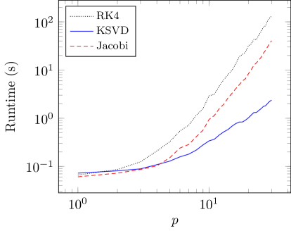
(a) Rectangular anisotropic mesh

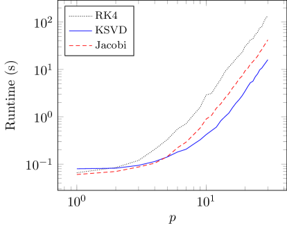
(b) Skewed anisotropic mesh

Figure 5: Wall-clock times for scalar advection on anisotropic meshes

Additionally, we measure the average wall-clock time required to both form and apply the Kronecker and block Jacobi preconditioners, for all polynomial degrees considered. We see that the cost of forming the Jacobi preconditioner quickly dominates the runtime. For large $p$, we begin to see the asymptotic $\mathcal{O}(p^{6})$ complexity for this operation. Applying the Jacobi preconditioner requires $\mathcal{O}(p^{4})$ operations, while both forming and applying the Kronecker preconditioner require $\mathcal{O}(p^{3})$ operations. These computational complexities are evident from the measured wall-clock times, shown in Figure 6.

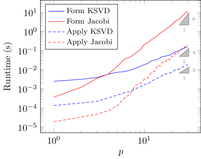
Figure 6: Wall-clock time required to form (solid lines) and apply (dashed lines) the exact block Jacobi and approximate Kronecker-product preconditioners.

5.3 2D Euler vortex

In this example, we consider the compressible Euler equations of gas dynamics in two dimensions, given in conservative form by

$$\partial_{t}\bm{u}+\nabla\cdot F(\bm{u})=0,$$ (68)

where

$$\bm{u}=\left(\begin{array}[]{c}\rho\\ \rho u\\ \rho v\\ \rho E\end{array}\right),\qquad F_{1}(\bm{u})=\left(\begin{array}[]{c}\rho u\\ \rho u^{2}+p\\ \rho uv\\ \rho Hu\end{array}\right),\qquad F_{2}(\bm{u})=\left(\begin{array}[]{c}\rho v\\ \rho uv\\ \rho v^{2}+p\\ \rho Hv\end{array}\right),$$ (69)

where $\rho$ is the density, $\bm{v}=(u,v)$ is the fluid velocity, $p$ is the pressure, and $E$ is the specific energy. The total enthalpy $H$ is given by

$$H=E+\frac{p}{\rho},$$ (70)

and the pressure is determined by the equation of state

$$p=(\gamma-1)\rho\left(E-\frac{1}{2}(u^{2}+v^{2})\right),$$ (71)

where $\gamma=c_{p}/c_{v}$ is the ratio of specific heat capacities at constant pressure and constant volume, taken to be 1.4.

We consider the model problem of an unsteady compressible vortex in a rectangular domain [37]. The domain is taken to be a $20\times 15$ rectangle and the vortex is initially centered at $(x_{0},y_{0})=(5,5)$. The vortex is moving with the free-stream at an angle of $\theta$. The exact solution is given by

$$u=u_{\infty}\left(\cos(\theta)-\frac{\epsilon((y-y_{0})-\overline{v}t)}{2\pi r_{c}}\exp\left(\frac{f(x,y,t)}{2}\right)\right),$$ (72)

$$u=u_{\infty}\left(\sin(\theta)-\frac{\epsilon((x-x_{0})-\overline{u}t)}{2\pi r_{c}}\exp\left(\frac{f(x,y,t)}{2}\right)\right),$$ (73)

$$\rho=\rho_{\infty}\left(1-\frac{\epsilon^{2}(\gamma-1)M^{2}_{\infty}}{8\pi^{2}}\exp(f(x,y,t))\right)^{\frac{1}{\gamma-1}},$$ (74)

$$p=p_{\infty}\left(1-\frac{\epsilon^{2}(\gamma-1)M^{2}_{\infty}}{8\pi^{2}}\exp(f(x,y,t))\right)^{\frac{\gamma}{\gamma-1}},$$ (75)

where $f(x,y,t)=(1-((x-x_{0})-\overline{u}t)^{2}-((y-y_{0})-\overline{v}t)^{2})/r_{c}^{2}$, $M_{\infty}$ is the Mach number, $u_{\infty},\rho_{\infty},$ and $p_{\infty}$ are the free-stream velocity, density, and pressure, respectively. The free-stream velocity is given by $(\overline{u},\overline{v})=u_{\infty}(\cos(\theta),\sin(\theta))$. The strength of the vortex is given by $\epsilon$, and its size is $r_{c}$. We choose the parameters to be $M_{\infty}=0.5$, $u_{\infty}=1$, $\theta=\arctan(1/2)$, $\epsilon=0.3$, and $r_{c}=1.5$.

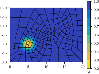
Figure 7: Initial conditions (density) for Euler vortex on unstructured mesh.

As in the case of the linear advection equation, we consider both a regular $n_{x}\times n_{y}$ cartesian grid, and an unstructured mesh. The unstructured mesh is obtained by scaling the mesh in Figure 2(b) by 20 in the $x$-direction and 15 in the $y$-direction. Density contours of the initial conditions are shown in Figure 7. As opposed to the scalar advection equation, the solution to the Euler equations consists of multiple components. Thus, the blocks of the Jacobian matrix can be considered to be of size $n_{c}(p+1)^{2}\times n_{c}(p+1)^{2}$, where $n_{c}$ is the number of solution components (in the case of the 2D Euler equations, $n_{c}=4$). The exact block Jacobi preconditioner computes the inverses of these large blocks. The approximate Kronecker-product preconditioner find optimal approximation of the form $A_{1}\otimes B_{1}+A_{2}\otimes B_{2}$, where $A_{1}$ and $A_{2}$ are $n_{c}(p+1)\times n_{c}(p+1)$ matrices, and $B_{1}$ and $B_{2}$ are $(p+1)\times(p+1)$ matrices.

We choose two representative time steps of $\Delta t=0.1$ and $\Delta t=0.01$, and compute the average number of GMRES iterations per linear solve required to perform one backward Euler time step. We choose the polynomial degree $p=3,4,\ldots,15$, and consider cartesian and unstructured meshes, both with 160 quadrilateral elements. We present the results in Table 3. Very similar results are observed for the structured and unstructured results. We note that for the smaller time step, the approximate Kronecker-product preconditioner requires a very similar number of iterations when compared with the exact block Jacobi preconditioner, even for high polynomial degree $p$. For the larger time step, the number of iterations required for the KSVD preconditioner increases with $p$ at a faster rate when compared with the block Jacobi preconditioner, suggesting that the Kronecker-product preconditioner is most effective for moderate time steps $\Delta t$.

Table 3: Number of GMRES iterations for Jacobi (J) and KSVD (K) preconditioners, Euler equations on cartesian and unstructured grids, with $\Delta t=0.1$ and $\Delta t=0.01$.

(a) Cartesian grid

	$\Delta t=0.01$		$\Delta t=0.1$
$p$	J	K	J	K
3	5	6	11	18
4	6	7	12	23
5	6	8	13	30
6	7	9	15	38
7	7	10	17	47
8	8	11	18	59
9	8	13	20	71
10	9	15	21	88
11	9	17	23	103
12	10	19	25	121
13	11	20	24	123
14	11	23	25	157
15	12	25	26	196

(b) Unstructured mesh

	$\Delta t=0.01$		$\Delta t=0.1$
$p$	J	K	J	K
3	6	7	12	19
4	6	7	14	26
5	7	9	16	32
6	7	10	17	42
7	8	11	18	51
8	8	12	20	64
9	9	13	21	74
10	9	15	23	90
11	9	17	24	110
12	10	19	25	125
13	10	21	25	142
14	11	24	26	164
15	11	26	27	245

5.3.1 Performance comparison

In this section we compare the runtime performance of the Kronecker-product preconditioner with the exact block Jacobi preconditioner. Although we have observed that for large time steps $\Delta t$ or polynomial degrees $p$, the KSVD preconditioner requires more iterations to converge, it is also possible to compute and apply this preconditioner much more efficiently. Here, we compare the wall-clock time required to compute and apply the preconditioner, according to Algorithms 5 and 6, respectively, for $p=3,4,\ldots,15$. The block Jacobi preconditioner is computed by first assembling the diagonal block of the Jacobian matrix using the sum-factorized form of expression (26), and then computing its LU factorization. The wall-clock times for these operations are shown in Figure 8(a). We remark that we observe the expected asymptotic computational complexities for each of these operations, where forming the Jacobi preconditioner requires $\mathcal{O}(p^{6})$ operations, and applying the Jacobi preconditioner requires $\mathcal{O}(p^{4})$ operations. Both forming and applying the approximate Kronecker-product preconditioner can be done in $\mathcal{O}(p^{3})$ time. The total runtime observed per backward Euler step for $\Delta t=0.1$ and $\Delta t=0.01$ is shown in Figure 8(b). We see that for $p\geq 7$ and $\Delta t=0.01$, the Kronecker-product preconditioner results in overall faster runtime, while for $\Delta t=0.1$, because of the large number of iterations required per solve, the Jacobi preconditioner results in overall faster performance.

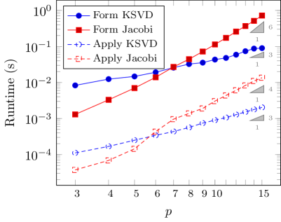
(a) Wall-clock time required to form and apply the KSVD and Jacobi preconditioners

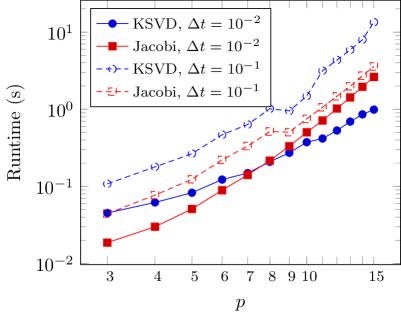
(b) Total wall-clock time required per backward Euler step

Figure 8: Runtime performance comparison of Kronecker-product preconditioner with exact block Jacobi preconditioner for 2D Euler equations.

5.4 2D Kelvin-Helmholtz instability

For a more sophisticated test case, we consider a two-dimensional Kelvin-Helmholtz instability. This important fluid instability occurs in shear flows of fluids with different densities. The domain is taken to be the periodic unit square $[0,1]^{2}$.

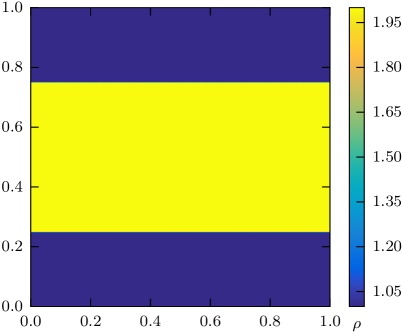
(a) Density

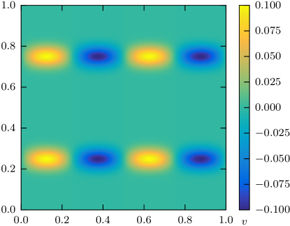
(b) Vertical velocity

Figure 9: Initial conditions for the Kelvin-Helmholtz instability.

We define the function

$$f(x)=\frac{1}{4}(\operatorname{erf}(\alpha(x-0.25))+1)(\operatorname{erf}(\alpha(0.75-x))+1),$$ (76)

where $\alpha=100$, as a smooth approximation to the discontinuous characteristic function

$$\chi(x)=\begin{cases}1,&\qquad 0.25\leq x\leq 0.75\\ 0,&\qquad\text{otherwise.}\end{cases}$$ (77)

Following [33], we define the initial conditions by

$$\rho(x,y)=f(y)+1,\qquad u(x,y)=f(y)-1/2,\qquad p(x,y)=2.5,$$ (78)

where the vertical velocity is given by

$$v(x,y)=\frac{1}{10}\sin(4\pi x)\left(\exp\left(-\frac{(y-0.25)^{2}}{2\sigma^{2}}\right)+\exp\left(-\frac{(y-0.75)^{2}}{2\sigma^{2}}\right)\right).$$ (79)

Thus, the fluid density is equal to 2 inside the strip $y\in[0.25,0.75]$, and 1 outside the strip. The fluid is moving to the right with horizontal velocity 0.5 inside the strip, and is moving to the left with equal speed outside of the strip. A small perturbation in the vertical velocity, localized around the discontinuity, determines the large-scale behavior of the instability. The initial conditions are shown in Figure 9.

We use a $128\times 128$ cartesian grid, with polynomial bases of degree 3, 7, and 10. For 10th degree polynomials, the total number of degrees of freedom is 7,929,856. The Euler equations are integrated for $1.5~{}\rm s$ using a fourth-order explicit method with a time step of $\Delta t=2.5\times 10^{-5}$ on the NERSC Edison supercomputer, using 480 cores. At this point, the solution has developed sophisticated large- and small-scale features, as shown in Figure 10.

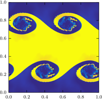
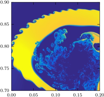
Figure 10: Solution (density) of Kelvin-Helmholtz instability at $t=1.5~{}\rm s$, with zoomed-in subregion to show small-scale features.

We then linearize the Euler equations around this solution in order to test the preconditioner performance. Because of the varied scale of the features in this solution, we believe that the resulting linearization is a representative of the DG systems we are interested in solving. Using this solution, we then solve one backward Euler step using both the Jacobi and approximate Kronecker-product preconditioners. For the implicit solve, we choose a range of time steps, from the explicit step size of $\Delta t=2.5\times 10^{-5}$, to a larger step of $\Delta t=10^{-3}$. The number of GMRES iterations required per linear solve are show in Table 4. We observe that for the explicit-scale time step, the exact block Jacobi and approximation Kronecker-product preconditioner exhibit very similar performance for all choices of $p$. For the largest time step, $\Delta t=10^{-3}$, the Kronecker-product preconditioner required about twice as many iterations for $p=3$, three times as many for $p=7$, and four times as many iterations for $p=10$.

Table 4: Number of GMRES iterations for Jacobi (J) and KSVD (K) preconditioners, Euler equations for 2D Kelvin-Helmholtz instability.

$p=3$

$\Delta t$	J	K
$2.5\times 10^{-5}$	4	4
$5.0\times 10^{-5}$	5	5
$1.0\times 10^{-4}$	6	7
$2.5\times 10^{-4}$	8	10
$5.0\times 10^{-4}$	10	14
$1.0\times 10^{-3}$	13	22

$p=7$

$\Delta t$	J	K
$2.5\times 10^{-5}$	5	6
$5.0\times 10^{-5}$	6	8
$1.0\times 10^{-4}$	8	12
$2.5\times 10^{-4}$	12	20
$5.0\times 10^{-4}$	15	35
$1.0\times 10^{-3}$	21	62

$p=10$

$\Delta t$	J	K
$2.5\times 10^{-5}$	6	8
$5.0\times 10^{-5}$	8	11
$1.0\times 10^{-4}$	10	16
$2.5\times 10^{-4}$	14	31
$5.0\times 10^{-4}$	19	55
$1.0\times 10^{-3}$	24	106

5.5 2D NACA Airfoil

In this test case, we consider the viscous flow over a NACA 0012 airfoil with angle of attack $30^{\circ}$ at Reynolds number 16000, with Mach number $M_{0}=0.2$. We take the domain to be a disk of radius 10, centered at (0,0). The leading edge of the airfoil is placed at the origin. A no-slip wall condition is enforced at the surface of the airfoil, and far-field conditions are enforced at all other domain boundaries. The far-field velocity is set to unity in the freestream direction. The domain is discretized using an unstructured quadrilateral mesh, refined in the vicinity of the wing and in its wake. Isoparametric mappings are used to curve the elements on the airfoil surface. This flow is characterized by the thin boundary layer that develops on the airfoil. In order to resolve this boundary layer, we introduce stretched, anisotropic boundary-layer elements at the surface of the airfoil. These small elements result in a CFL condition that requires the use of very small time steps when using an explicit time integration method. The mesh and density contours are shown in Figure 11.

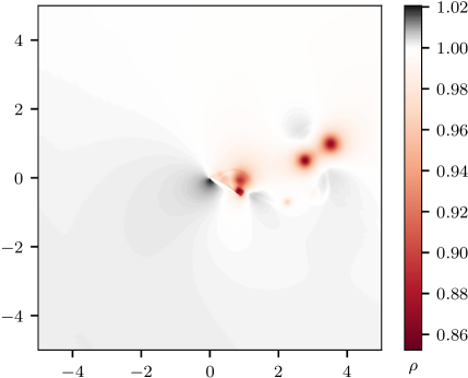
Figure 11: NACA 0012 mesh, with zoom-in around the surface of the airfoil showing anisotropic boundary-layer elements (top), and solution (density).

This test case differs from the preceding two test cases because instead of the Euler equations we solve the compressible Navier-Stokes equations,

$$\frac{\partial\rho}{\partial t}+\frac{\partial}{\partial x_{j}}(\rho u_{j})=0$$ (80)

$$\frac{\partial}{\partial t}(\rho u_{i})+\frac{\partial}{\partial x_{j}}(\rho u_{i}u_{j})+\frac{\partial p}{\partial x_{i}1}=\frac{\partial\tau_{ij}}{\partial x_{j}}\qquad\text{for $i=1,2,3,$}$$ (81)

$$\frac{\partial}{\partial t}(\rho E)+\frac{\partial}{\partial x_{j}}\left(u_{j}(\rho E+p)\right)=-\frac{\partial q_{j}}{\partial x_{j}}+\frac{\partial}{\partial x_{j}}(u_{j}\tau_{ij}),$$ (82)

The viscous stress tensor and heat flux are given by

$$\tau_{ij}=\mu\left(\frac{\partial u_{i}}{\partial x_{j}}+\frac{\partial u_{j}}{\partial x_{i}}-\frac{2}{3}\frac{\partial u_{k}}{\partial x_{k}}\delta_{ij}\right)\qquad\text{and}\qquad q_{j}=-\frac{\mu}{\rm Pr}\frac{\partial}{\partial x_{j}}\left(E+\frac{p}{\rho}-\frac{1}{2}u_{k}u_{k}\right).$$ (83)

Here $\mu$ is the coefficient of viscosity, and ${\rm Pr}$ is the Prandtl number, which we assume to be constant. We discretize the second-order terms using the local discontinuous Galerkin method [7], which introduces certain lifting operators into the primal form of the discretization [2]. These lifting operators do not readily fit into the tensor-produce framework described above, and thus we apply the approximate Kronecker-product preconditioner to only the inviscid component of the flux function. Since the flow is convection-dominated away from the airfoil, we believe that this provides an acceptable approximation, although properly incorporating the viscous terms into the preconditioner is an area of ongoing research.

We integrate the equations until $t=2.5$ in order to obtain a representative initial condition about which to linearize the equations. We consider polynomial degrees $p=1,3,7,10,15$, and compare the efficiency of explicit and implicit time integration methods, using both the Kronecker-product preconditioner and exact block Jacobi. In order to make this comparison, we determine experimentally the largest explicit timestep for which the system is stable. Then, we measure the wall-clock time required to integrate the system from $t=2.5$ until $t=3.5$. Similarly, for the implicit methods, we experimentally choose an appropriate $\Delta t$ measure the wall-clock time required to advance the simulation until $t=3.5$ using a three-stage, third-order, $L$-stable DIRK scheme. We present these results in Table 5. We note that for $p>3$, the Kronecker-product preconditioner results in the shortest runtimes. For large $p$, the exact block Jacobi preconditioner becomes impractical due to the large $p$-dependence of the computational complexity. For $p=15$, the high degree polynomials considered for this test case, the Kronecker preconditioner resulted in runtimes that were about a factor of two faster than explicit, and a factor of ten faster than exact block Jacobi.

			Runtime (s)
$p$	Explicit $\Delta t$	Implicit $\Delta t$	RK4	K	J
1	$1.0\times 10^{-4}$	$2.0\times 10^{-1}$	$8.864\times 10^{1}$	$5.225\times 10^{1}$	$5.854\times 10^{1}$
3	$2.5\times 10^{-5}$	$5.0\times 10^{-2}$	$6.381\times 10^{2}$	$8.406\times 10^{2}$	$4.626\times 10^{2}$
7	$1.0\times 10^{-6}$	$2.0\times 10^{-3}$	$5.441\times 10^{4}$	$3.057\times 10^{4}$	$6.765\times 10^{4}$
10	$5.0\times 10^{-7}$	$2.5\times 10^{-4}$	$2.218\times 10^{5}$	$1.884\times 10^{5}$	$1.949\times 10^{6}$
15	$1.0\times 10^{-7}$	$2.0\times 10^{-4}$	$2.372\times 10^{6}$	$1.176\times 10^{6}$	$1.223\times 10^{7}$

Table 5: Runtime results for NACA test-case, comparing explicit (fourth-order Runge-Kutta) with implicit (three-stage DIRK), using Kronecker and exact block Jacobi preconditioners. Runtime in seconds per simulation second is presented.

5.6 3D periodic Euler

In this example, we provide a test case for the three-dimensional preconditioner. We consider the cube $[0,2]^{3}$ with periodic boundary conditions, and use the initial conditions from [17], given by

$$\rho=1+0.2\sin(\pi(x+y+z)),$$ (84)

$$u=1,\quad v=-1/2,\quad w=1,$$ (85)

$$p=1.$$ (86)

The exact solution to the Euler equations is known analytically in this case. Velocity and pressure remain constant in time, and the density at time $t$ is given by

$$\rho=1+0.2\sin(\pi(x+y+z-t(u+v+w))).$$ (87)

The initial conditions are shown in Figure 12. The mesh is taken to be a regular $6\times 6\times 6$ hexahedral grid, and we consider polynomial degrees of $p=1,2,\ldots,12$. We choose a representative time step of $\Delta t=2.5\times 10^{-3}$. This time step can be used for explicit methods with low-degree polynomials, but because of the $p$-dependency of the CFL condition, we observe that for $p\geq 9$, explicit methods become unstable, motivating the use of implicit methods. In order to compare the efficiency of the approximate Kronecker-product preconditioner, we compute one backward Euler step and compare the number of GMRES iterations required per linear solve using the exact block Jacobi preconditioner and the KSVD preconditioner.

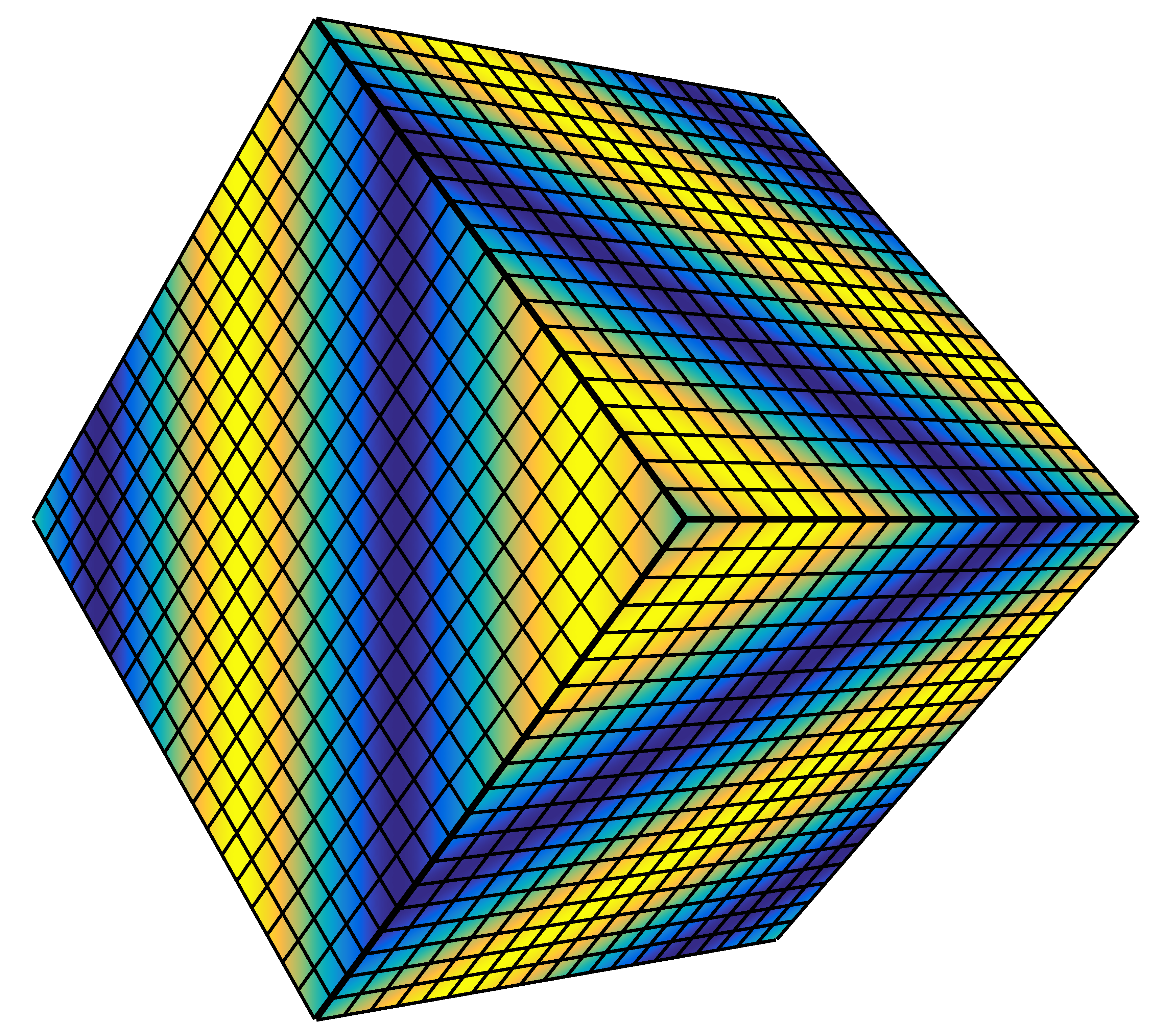
Figure 12: Initial conditions (density) for smooth 3D Euler test case.

In this test case, we also consider two variations each of these preconditioners. Since the solution to the Euler equations consists of five components, we can consider the diagonal blocks of the Jacobian to either be large $5(p+1)^{3}\times 5(p+1)^{3}$ blocks coupling all solution components, or as smaller $(p+1)^{3}\times(p+1)^{3}$ blocks, which do not couple the solution components. We expect that using the smaller blocks will require more GMRES iterations per linear solve, because each block captures less information. The larger blocks, on the other hand, are much more computationally expensive to compute. We present the number of iterations required to converge for each of the preconditioners in Table 14, where $J$ and $K$ stand for the block Jacobi and Kronecker-product preconditioners, respectively, and the subscripts “full” and “small” refer to the block size used. We observe that for small polynomial degree $p$, the KSVD preconditioner results in close-to-identical number of iterations, when compared with exact block Jacobi. For this test case, for $p$ closer to 12, we observe that the number of iterations grows faster for the KSVD preconditioner than for the block Jacobi preconditioner, but the difference remains relatively small. Additionally, as expected, the small-block preconditioner requires a greater number of iterations to converge when compared with the full-block preconditioner. We note that due to the very large memory requirements, the full Jacobi preconditioner did not complete for $p=12$.

$p$	$J_{\rm full}$	$K_{\rm full}$	$J_{\rm small}$	$K_{\rm small}$
1	4	4	5	5
2	4	5	6	6
3	5	5	7	7
4	5	5	8	8
5	5	6	9	10
6	5	6	11	12
7	5	6	12	13
8	5	7	15	16
9	5	7	16	17
10	5	8	19	21
11	5	8	20	22
12	-	9	23	26

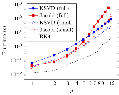
Figure 13: GMRES iterations required per linear solve for three-dimensional periodic Euler test case.

Figure 14: Wall-clock time required per backward Euler solve for three-dimensional periodic Euler test case. For reference, wall-clock time required for explicit RK4 is shown.

We additionally measure the wall-clock time required per backward Euler step for each of the preconditioners, and present the results in Figure 14. For reference, we also include the wall-clock time required to integrate the system of equations for an equivalent time using the explicit RK4 method with a stable time step. This problem is well-suited for explicit solvers, and thus the RK4 method is more efficient than the implicit methods. From these measurements, it is possible to draw several conclusions. Firstly, as $p$ grows, it becomes possible to observe the $\mathcal{O}(p^{9})$ complexity of the exact block Jacobi preconditioner, which becomes prohibitively expensive. This is in contrast to the Kronecker-product preconditioner, whose $\mathcal{O}(p^{5})$ complexity results in reasonable runtimes for all $p$ considered. The full-block KSVD preconditioner results in faster runtimes starting at about $p=5$, and the small-block preconditioner at about $p=4$. We also see that, despite the larger number of iterations required, the small-block preconditioner results in faster overall runtime.

5.7 Compressible Taylor-Green Vortex at ${\rm Re}=1600$

The direct numerical simulation of the Taylor-Green vortex at ${\rm Re}=1600$ is a benchmark problem from the first International Workshop on High-Order CFD Methods [37]. This three-dimensional problem has been often used to study the performance of high-order methods, and DG methods in particular, on transitional flows. This problem provides a useful test case because of the availability of fully-resolved reference data [32, 35, 5, 10, 6]. The domain is taken to be the periodic cube $[-\pi,\pi]^{3}$. The initial conditions are given by

$$u(x,y,z) =u_{0}\sin(x)\cos(y)\cos(z)$$ (88)

$$v(x,y,z) =-u_{0}\cos(x)\sin(y)\cos(z)$$ (89)

$$w(x,y,z) =0$$ (90)

$$p(x,y,z) =p_{0}+\frac{\rho_{0}u_{0}^{2}}{16}\left(\cos(2x)+\cos(2y)\right)\left(\cos(2z)+2\right),$$ (91)

where the parameters are given by $\gamma=1.4$, ${\rm Pr}=0.71$, $u_{0}=1$, $\rho_{0}=1$, with Mach number $M_{0}=u_{0}/c_{0}=0.10$, where $c_{0}$ is the speed of sound computed in accordance with the pressure $p_{0}$. The initial density distribution is then given by $\rho=p\rho_{0}/p_{0}$. The characteristic convective time is given by $t_{\rm c}=1$, and the final time is $t_{\rm f}=20t_{\rm c}$. The geometry is discretized using regular hexahedral grids of size $8^{3},16^{3},32^{3},$ and $42^{3}$, with polynomial degrees $p=3,4,7,$ and $15$.

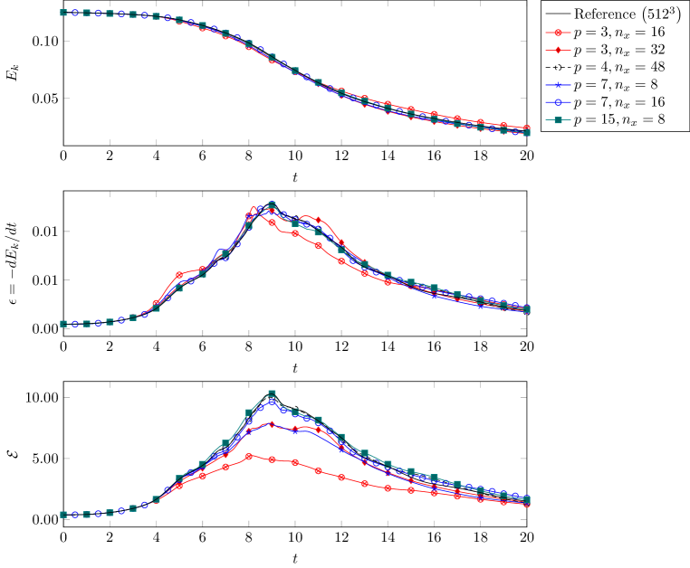
Figure 15: Time evolution of kinetic energy $E_{k}$, kinetic energy dissipation rate (KEDR) $\epsilon$, and enstrophy $\mathcal{E}$, for Taylor-Green test case. Comparison of various DG configurations with reference pseudo-spectral solution.

The Taylor-Green vortex provides a strong motivation for the use of very high polynomial degrees. In Figure 15, we show the time-evolution of the diagnostic quantities of mean energy, kinetic energy dissipation rate, and enstrophy,

$$E_{k}(t) =\frac{1}{\rho_{0}|\Omega|}\int_{\Omega}\rho\frac{\bm{u}\cdot\bm{u}}{2}~{}dx,$$ (92)

$$\epsilon(t) =-\frac{dE_{k}}{dt}(t),$$ (93)

$$\mathcal{E}(t) =\frac{1}{\rho_{0}|\Omega|}\int_{\Omega}\rho\frac{\omega\cdot\omega}{2}~{}dx.$$ (94)

For each grid configuration, we compare the results with a fully-resolved pseudo-spectral reference solution. We notice that the relatively low-order solutions with $p=3$ severely underpredict the peak enstrophy. However, with equal numbers of numerical degrees of freedom, the higher-order $p=7$ and $p=15$ solutions much more closely match the reference data. For example, the $n_{x}=8,p=15$ discretization results in much better agreement than the $n_{x}=32,p=3$ case, despite an equal number of degrees of freedom, motivating the use of very high polynomial degrees.

We now examine the efficiency of the approximate tensor-product preconditioner compared with exact block Jacobi for each of the grid configurations shown in Figure 15. For each configuration, we choose a range of timesteps, ranging from $\Delta t=10^{-4}$ to $\Delta t=1.6\times 10^{-3}$ by factors of two. We measure the average number of GMRES iterations per linear solve, and list the results in Table 6. In the case of the $p=15,n_{x}=8$, the exact block Jacobi preconditioner did not complete because of excessive runtime and memory requirements. These iteration counts indicate that the number of GMRES iterations per linear solve increases as the timestep increases, and that this dependence is sublinear. For almost all cases, the Kronecker-product preconditioner resulted in very similar to iteration counts when compared with exact block Jacobi. However, due to the decreased computational complexity and decreased memory requirements, the KSVD preconditioner can be used to obtain similar GMRES convergence at a highly decreased computational cost.

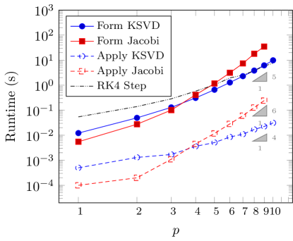
Figure 16: Wall-clock time required to form (solid lines) and apply (dashed lines) the exact block Jacobi and approximate Kronecker-product preconditioners. For reference, also shown is time per RK4 step.

In Figure 16, we show the wall-clock times required to form and apply the approximate Kronecker and exact block Jacobi preconditioners with $n_{x}=8$ and $p=1,2,\ldots,10.$ Due to excessive memory requirements, the exact Jacobi preconditioner was not computed for $p=10$. The improved computational complexities for the KSVD preconditioner for both operations are apparent. Forming the Kronecker-product preconditioner requires $\mathcal{O}(p^{5})$ operations and applying the preconditioner requires $\mathcal{O}(p^{4})$ operations, as opposed to $\mathcal{O}(p^{9})$ and $\mathcal{O}(p^{6})$, respectively, for the block Jacobi preconditioner. For comparison, the wall-clock time required to perform one explicit RK4 step is also shown. By taking advantage of the tensor-product structure, as described in Section 3.3, the computational complexity of performing an explicit step scales as $\mathcal{O}(p^{4})$. However, the choice of stable time step is severely restricted as $p$ grows, requiring a large number of steps to be taken. This problem is structurally quite similar to that of Section 5.6, since the geometry for both problems is a regular cartesian grid, and the equations only differ in the presence of viscosity. Therefore, the performance characteristics for the solvers are quite similar to those shown in Figure 14. For example, we observe that for $p=7,n_{x}=8$, the explicit time integration results in an overall runtime that is about one-fifth of the runtime for implicit time integration with the KSVD preconditioner, and one-seventh of the runtime for implicit time integration with the block Jacobi preconditioner.

Table 6: Average number of GMRES iterations per linear solve for Taylor-Green test case.

(a) $p=3,n_{x}=16$

$\Delta t$	Jacobi	KSVD
$1\times 10^{-4}$	4	4
$2\times 10^{-4}$	5	7
$4\times 10^{-4}$	6	7
$8\times 10^{-4}$	8	9
$1.6\times 10^{-3}$	11	12

(b) $p=3,n_{x}=32$

$\Delta t$	Jacobi	KSVD
$1\times 10^{-4}$	5	5
$2\times 10^{-4}$	6	6
$4\times 10^{-4}$	7	8
$8\times 10^{-4}$	10	12
$1.6\times 10^{-3}$	16	18

(c) $p=4,n_{x}=48$

$\Delta t$	Jacobi	KSVD
$1\times 10^{-4}$	7	7
$2\times 10^{-4}$	9	10
$4\times 10^{-4}$	12	16
$8\times 10^{-4}$	19	27
$1.6\times 10^{-3}$	30	40

(d) $p=7,n_{x}=8$

$\Delta t$	Jacobi	KSVD
$1\times 10^{-4}$	5	6
$2\times 10^{-4}$	6	6
$4\times 10^{-4}$	8	8
$8\times 10^{-4}$	10	11
$1.6\times 10^{-3}$	15	16

(e) $p=7,n_{x}=16$

$\Delta t$	Jacobi	KSVD
$1\times 10^{-4}$	6	6
$2\times 10^{-4}$	7	9
$4\times 10^{-4}$	10	13
$8\times 10^{-4}$	15	17
$1.6\times 10^{-3}$	25	29

(f) $p=15,n_{x}=8$

$\Delta t$	Jacobi	KSVD
$1\times 10^{-4}$	–	8
$2\times 10^{-4}$	–	11
$4\times 10^{-4}$	–	15
$8\times 10^{-4}$	–	26
$1.6\times 10^{-3}$	–	88

6 Conclusion and future work

In this work we have developed new approximate tensor-product based preconditioners for very high-order discontinuous Galerkin methods. These preconditioners are computed using an algebraic singular value-based algorithm, and compare favorably with the traditional block Jacobi preconditioner. The computational complexity is reduced from $\mathcal{O}(p^{6})$ to $\mathcal{O}(p^{3})$ in two spatial dimensions and $\mathcal{O}(p^{9})$ to $\mathcal{O}(p^{5})$ in three spatial dimensions. Numerical results in two and three dimensions for the advection and Euler equations, using polynomial degrees up to $p=30$, confirm the expected computational complexities, and demonstrate significant reductions in runtimes for certain test problems.

Future work for further improving the performance of this preconditioner include systematic treatment of viscous fluxes and second-order terms, and fast inversion of sums of more than two Kronecker products allowing for treatment of off-diagonal blocks in the context of an ILU-based preconditioner. Also of interest is the investigation of the performance of the preconditioner when used as a smoother in $p$-multigrid solvers.

7 Acknowledgments

This research used resources of the National Energy Research Scientific Computing Center, a DOE Office of Science User Facility supported by the Office of Science of the U.S. Department of Energy under Contract No. DE-AC02-05CH11231, and was supported by the AFOSR Computational Mathematics program under grant number FA9550-15-1-0010. The first author was supported by the Department of Defense through the National Defense Science & Engineering Graduate Fellowship Program and by the Natural Sciences and Engineering Research Council of Canada.

References

- [1] Roger Alexander. Diagonally implicit Runge-Kutta methods for stiff O.D.E.’s. SIAM Journal on Numerical Analysis, 14(6):1006–1021, 1977.
- [2] Douglas N. Arnold, Franco Brezzi, Bernardo Cockburn, and L. Donatella Marini. Unified analysis of discontinuous Galerkin methods for elliptic problems. SIAM Journal on Numerical Analysis, 39(5):1749–1779, 2002.
- [3] Abdalkader Baggag, Harold Atkins, and David Keyes. Parallel implementation of the discontinuous galerkin method. 1999.
- [4] Philipp Birken, Gregor Gassner, Mark Haas, and Claus-Dieter Munz. Preconditioning for modal discontinuous Galerkin methods for unsteady 3D Navier-Stokes equations. Journal of Computational Physics, 240:20–35, may 2013.
- [5] C. Carton de Wiart, K. Hillewaert, M. Duponcheel, and G. Winckelmans. Assessment of a discontinuous Galerkin method for the simulation of vortical flows at high Reynolds number. International Journal for Numerical Methods in Fluids, 74(7):469–493, 2014.
- [6] Jean-Baptiste Chapelier, Marta De La Llave Plata, and Florent Renac. Inviscid and viscous simulations of the Taylor-Green vortex flow using a modal discontinuous Galerkin approach. In 42nd AIAA Fluid Dynamics Conference and Exhibit. American Institute of Aeronautics and Astronautics, June 2012.
- [7] Bernardo Cockburn and Chi-Wang Shu. The local discontinuous Galerkin method for time-dependent convection-diffusion systems. SIAM Journal on Numerical Analysis, 35(6):2440–2463, 1998.
- [8] Bernardo Cockburn and Chi-Wang Shu. The Runge-Kutta discontinuous Galerkin method for conservation laws V: multidimensional systems. Journal of Computational Physics, 141(2):199–224, 1998.
- [9] A. Crivellini and F. Bassi. An implicit matrix-free discontinuous Galerkin solver for viscous and turbulent aerodynamic simulations. Computers & Fluids, 50(1):81–93, nov 2011.
- [10] James DeBonis. Solutions of the Taylor-Green vortex problem using high-resolution explicit finite difference methods. In 51st AIAA Aerospace Sciences Meeting including the New Horizons Forum and Aerospace Exposition. American Institute of Aeronautics and Astronautics, January 2013.
- [11] Laslo T. Diosady. Domain Decomposition Preconditioners for Higher-Order Discontinuous Galerkin Discretizations. PhD thesis, Massachusetts Institute of Technology, 2011.
- [12] Laslo T. Diosady and Scott M. Murman. Tensor-product preconditioners for higher-order space–time discontinuous Galerkin methods. Journal of Computational Physics, 330:296 – 318, 2017.
- [13] J. A. Escobar-Vargas, P. J. Diamessis, and C. F. Van Loan. The numerical solution of the pressure Poisson equation for the incompressible Navier-Stokes equations using a quadrilateral spectral multidomain penalty method. Preprint available at https://www.cs.cornell.edu/cv/ResearchPDF/Poisson.pdf, 2011.
- [14] Gene H. Golub, Franklin T. Luk, and Michael L. Overton. A block Lanczos method for computing the singular values and corresponding singular vectors of a matrix. ACM Transactions on Mathematical Software (TOMS), 7(2):149–169, 1981.
- [15] J. Gopalakrishnan and G. Kanschat. A multilevel discontinuous galerkin method. Numerische Mathematik, 95(3):527–550, 2003.
- [16] David Gottlieb and Eitan Tadmor. The CFL condition for spectral approximations to hyperbolic initial-boundary value problems. Mathematics of Computation, 56(194):565–588, 1991.
- [17] Guang-Shan Jiang and Chi-Wang Shu. Efficient implementation of weighted ENO schemes. Journal of Computational Physics, 126(1):202 – 228, 1996.
- [18] Guido Kanschat. Robust smoothers for high-order discontinuous Galerkin discretizations of advection–diffusion problems. Journal of Computational and Applied Mathematics, 218(1):53 – 60, 2008.
- [19] Robert Klöfkorn. Efficient matrix-free implementation of discontinuous Galerkin methods for compressible flow problems. In Proceedings of the Conference Algoritmy, pages 11–21, 2015.
- [20] Lilia Krivodonova and Ruibin Qin. An analysis of the spectrum of the discontinuous Galerkin method. Applied Numerical Mathematics, 64:1–18, 2013.
- [21] M. Kronbichler, S. Schoeder, C. Müller, and W. A. Wall. Comparison of implicit and explicit hybridizable discontinuous galerkin methods for the acoustic wave equation. International Journal for Numerical Methods in Engineering, 106(9):712–739, 2016. nme.5137.
- [22] Charles F. Van Loan. The ubiquitous Kronecker product. Journal of Computational and Applied Mathematics, 123(1–2):85 – 100, 2000. Numerical Analysis 2000. Vol. III: Linear Algebra.
- [23] Robert E. Lynch, John R. Rice, and Donald H. Thomas. Direct solution of partial difference equations by tensor product methods. Numerische Mathematik, 6(1):185–199, 1964.
- [24] K.-A. Mardal, T. K. Nilssen, and G. A. Staff. Order-optimal preconditioners for implicit Runge-Kutta schemes applied to parabolic PDEs. SIAM Journal on Scientific Computing, 29(1):361–375, 2007.
- [25] Steven A. Orszag. Spectral methods for problems in complex geometries. Journal of Computational Physics, 37(1):70 – 92, 1980.
- [26] Jaime Peraire and Per-Olof Persson. High-order discontinuous Galerkin methods for CFD. In Z. J. Wang, editor, Adaptive High-Order Methods in Fluid Dynamics, chapter 5, pages 119–152. World Scientific, 2011.
- [27] Per-Olof Persson and Jaime Peraire. An efficient low memory implicit DG algorithm for time dependent problems. In 44th AIAA Aerospace Sciences Meeting and Exhibit, page 113, 2006.
- [28] Per-Olof Persson and Jaime Peraire. Newton-GMRES preconditioning for discontinuous Galerkin discretizations of the Navier-Stokes equations. SIAM Journal on Scientific Computing, 30(6):2709–2733, 2008.
- [29] W. H. Reed and T. R. Hill. Triangular mesh methods for the neutron transport equation. Los Alamos Report LA-UR-73-479, 1973.
- [30] Yousef Saad. Iterative methods for sparse linear systems. SIAM, 2003.
- [31] Jie Shen, Tao Tang, and Li-Lian Wang. Separable Multi-Dimensional Domains, pages 299–366. Springer Berlin Heidelberg, Berlin, Heidelberg, 2011.
- [32] Chi-Wang Shu, Wai-Sun Don, David Gottlieb, Oleg Schilling, and Leland Jameson. Numerical convergence study of nearly incompressible, inviscid Taylor-Green vortex flow. Journal of Scientific Computing, 24(1):1–27, 2005.
- [33] Volker Springel. E pur si muove: Galilean-invariant cosmological hydrodynamical simulations on a moving mesh. Monthly Notices of the Royal Astronomical Society, 401(2):791, 2010.
- [34] Charles F. Van Loan and Nikos Pitsianis. Approximation with Kronecker products. In Linear Algebra for Large Scale and Real-Time Applications, pages 293–314. Springer, 1993.
- [35] Wim M. Van Rees, Anthony Leonard, D. I. Pullin, and Petros Koumoutsakos. A comparison of vortex and pseudo-spectral methods for the simulation of periodic vortical flows at high Reynolds numbers. Journal of Computational Physics, 230(8):2794–2805, 2011.
- [36] Peter E. J. Vos, Spencer J. Sherwin, and Robert M. Kirby. From to efficiently: Implementing finite and spectral/ element methods to achieve optimal performance for low-and high-order discretisations. Journal of Computational Physics, 229(13):5161–5181, 2010.
- [37] Z.J. Wang, Krzysztof Fidkowski, Rémi Abgrall, Francesco Bassi, Doru Caraeni, Andrew Cary, Herman Deconinck, Ralf Hartmann, Koen Hillewaert, H.T. Huynh, Norbert Kroll, Georg May, Per-Olof Persson, Bram van Leer, and Miguel Visbal. High-order CFD methods: current status and perspective. International Journal for Numerical Methods in Fluids, 72(8):811–845, 2013.
- [38] T. Warburton and T. Hagstrom. Taming the CFL number for discontinuous galerkin methods on structured meshes. SIAM Journal on Numerical Analysis, 46(6):3151–3180, jan 2008.
- [39] Masayuki Yano and David L. Darmofal. An optimization-based framework for anisotropic simplex mesh adaptation. Journal of Computational Physics, 231(22):7626–7649, 2012.
- [40] Matthew J. Zahr and Per-Olof Persson. Performance tuning of Newton-GMRES methods for discontinuous Galerkin discretizations of the Navier-Stokes equations. In 21st AIAA Computational Fluid Dynamics Conference. American Institute of Aeronautics and Astronautics, June 2013.