An unbalanced Optimal Transport splitting scheme for general advection-reaction-diffusion problems

T.O. Gallouët, M. Laborde, L. Monsaingeon
Résumé

In this paper, we show that unbalanced optimal transport provides a convenient framework to handle reaction and diffusion processes in a unified metric framework. We use a constructive method, alternating minimizing movements for the Wasserstein distance and for the Fisher-Rao distance, and prove existence of weak solutions for general scalar reaction-diffusion-advection equations. We extend the approach to systems of multiple interacting species, and also consider an application to a very degenerate diffusion problem involving a Gamma-limit. Moreover, some numerical simulations are included.

1 Introduction

Since the seminal works of Jordan-Kinderlehrer-Otto [19], it is well known that certain diffusion equations can be interpreted as gradient flows in the space of probability measures, endowed with the quadratic Wasserstein distance $\mathtt{W}$. The well-known JKO scheme (a.k.a. minimizing movement), which is a natural implicit Euler scheme for such gradient flows, naturally leads to constructive proofs of existence for weak solutions to equations or systems with mass conservation such as, for instance, Fokker-Planck equations [19], Porous Media Equations [32], aggregation equation [9], double degenerate diffusion equations [31], general degenerate parabolic equation [1] etc. We refer to the classical textbooks of Ambrosio, Gigli and Savaré [4] and to the books of Villani [43, 44] for a detailed account of the theory and extended bibliography. Recently, this theory has been extended to study the evolution of interacting species with mass-conservation, see for examples [15, 45, 23, 20, 8].

Nevertheless in biology, for example for diffusive prey-predator models, the conservation of mass may not hold, and the classical optimal transport theory does not apply. An unbalanced optimal transport theory was recently introduced simultaneously in [11, 12, 21, 25, 26], and the resulting Wasserstein-Fisher-Rao ($\mathtt{WFR}$) metrics (also referred to as the Hellinger-Kantorovich distance $\mathtt{HK}$) allows to compute distances between measures with variable masses while retaining a convenient Riemannian structure. See section 2 for the definition and a short discussions on this $\mathtt{WFR}$ metric. We also refer to [37, 16] for earlier attempts to account for mass variations within the framework of optimal transport.

The $\mathtt{WFR}$ metrics can be seen as an inf-convolution between Wasserstein/transport and Fisher-Rao/reaction processes, and is therefore extremely convenient to control both in a unified metric setting. This allows to deal with non-conservative models of population dynamics, see e.g. [21, 22]. In [18], the first and third authors proposed a variant of the JKO scheme for $\mathtt{WFR}$-gradient flows corresponding to some particular class of reaction-diffusion PDEs: roughly speaking, the reaction and diffusion were handled separately in two separate $\mathtt{FR},\mathtt{W}$ metrics, and then patched together using a particular uncoupling of the inf-convolution, namely $\mathtt{WFR}^{2}\approx\mathtt{W}^{2}+\mathtt{FR}^{2}$ in some sense (see [18, section 3] for a thorough discussion). However, the analysis was restricted to very particular structures for the PDE, corresponding to pure $\mathtt{WFR}$ gradient-flows.

In this work we aim at extending this splitting scheme in order to handle more general reaction-diffusion problems, not necessarily corresponding to gradient flows. Roughly speaking, the structure of our splitting scheme is the following: the transport/diffusion part of the PDE is treated by a single Wasserstein JKO step

$$\rho^{k}\xrightarrow[\mbox{transport}]{\mathtt{W}}\rho^{k+1/2},$$

and the next Fisher-Rao JKO step

$$\rho^{k+1/2}\xrightarrow[\mbox{reaction}]{\mathtt{FR}}\rho^{k+1}$$

handles the reaction part of the evolution. As already mentioned, the $\mathtt{WFR}$ metric will allow to suitable control both steps in a unified metric framework. We will first state a general convergence result for scalar reaction-diffusion equations, and then illustrate on a few particular examples how the general idea can be adapted to treat e.g. prey-predator systems or very degenerate Hele-Shaw diffusion problems. In this work we do not focus on optimal results and do not seek full generality, but rather wish to illustrate the efficiency of the general approach.

Another advantage of the splitting scheme is that is well adapted to existing Monge/Kantorovich/Wasserstein numerical solvers, and the Fisher-Rao step turns out to be a simple pointwise convex problem which can be implemented in a very simple way. See also [10, 13] for a more direct numerical approach by entropic regularization. Throughout the paper we will illustrate the theoretical results with a few numerical tests. All the numerical simulations were implemented with the augmented Lagrangian ALG2-JKO scheme from [6] for the Wasserstein step, and we used a classical Newton algorithm for the Fisher-Rao step.

The paper is organized as follows. In section 2 we recall the basic definitions and useful properties of the Wasserstein-Fisher-Rao distance $\mathtt{WFR}$. Section 3 contains the precise description of the splitting scheme and a detailed convergence analysis for a broad class of reaction-diffusion equations. In section 4 we present an extension to some prey-predator multicomponent systems with nonlocal interactions. In section 5 we extend the general result from section 3 to a very degenerate tumor growth model studied in [34], corresponding to a pure $\mathtt{WFR}$ gradient flow: we show that the splitting scheme captures fine properties of the model, particularly the $\Gamma$-convergence of discrete gradient flows as the degenerate diffusion parameter of Porous Medium type $m\to\infty$. The last section 6 contains an extension to a tumor-growth model coupled with an evolution equation for the nutrients.

2 Preliminaries

Let us first fix some notations. Throughout the whole paper, $\Omega$ denotes a possibly unbounded convex subset of $\operatorname*{\mathbb{R}}^{d}$, $Q_{T}$ represents the product space $[0,T]\times\Omega$, for $T>0$, and we write $\mathcal{M}^{+}=\mathcal{M}^{+}(\Omega)$ for the set of nonnegative finite Radon measures on $\Omega$. We say that a curve of measures $t\mapsto\rho_{t}\in\mathcal{C}_{w}([0,1];\mathcal{M}^{+})$ is narrowly continuous if it is continuous with respect to the narrow convergence of measures, namely for the duality with $\mathcal{C}_{b}(\Omega)$ test-functions.

Definition 2.1.

The Fisher-Rao distance between $\rho_{0},\rho_{1}\in\mathcal{M}^{+}$ is

$$\mathtt{FR}(\rho_{0},\rho_{1}):=\min_{(\rho_{t},r_{t})\in\mathcal{A}_{\mathtt{FR}}[\rho_{0},\rho_{1}]}\int_{0}^{1}\int_{\Omega}|r_{t}|^{2}\,d\rho_{t}(x)dt,$$

where the admissible set $A_{\mathtt{FR}}[\rho_{0},\rho_{1}]$ consists in curves $[0,1]\ni t\mapsto(\rho_{t},r_{t})\in\mathcal{M}^{+}\times\mathcal{M}$ such that $t\mapsto\rho_{t}\in\mathcal{C}_{w}([0,1];\mathcal{M}^{+})$ is narrowly continuous with endpoints $\rho_{t}(0)=\rho_{0},\rho_{t}(1)=\rho_{1}$, and

$$\partial_{t}\rho_{t}=\rho_{t}r_{t}$$

in the sense of distributions $\mathcal{D}^{\prime}((0,1)\times\Omega)$.

The Monge-Kantorovich-Wasserstein admits several equivalent definitions and formulations, and we refer e.g. to [43, 44, 4, 41] for a complete description. For our purpose we shall only need the dynamical Benamou-Brenier formula:

Theorem 2.2 (Benamou-Brenier formula, [5, 4]).

There holds

$$\mathtt{W}^{2}(\rho_{0},\rho_{1})=\min\limits_{(\rho,\mathbf{v})\in\mathcal{A}_{\mathtt{W}}[\rho_{0},\rho_{1}]}\int_{0}^{1}\int_{\Omega}|\mathbf{v}_{t}|^{2}\mathrm{d}\rho_{t}\mathrm{d}t,$$ (2.1)

where the admissible set $\mathcal{A}_{\mathtt{W}}[\rho_{0},\rho_{1}]$ consists in curves $(0,1)\ni t\mapsto(\rho_{t},\mathbf{v}_{t})\in\mathcal{M}^{+}\times\mathcal{M}(\Omega;\operatorname*{\mathbb{R}}^{d})$ such that $t\mapsto\rho_{t}$ is narrowly continuous with endpoints $\rho_{t}(0)=\rho_{0}$, $\rho_{t}(1)=\rho_{1}$ and solving the continuity equation

$$\partial_{t}\rho_{t}+\operatorname*{div}(\rho_{t}\mathbf{v}_{t})=0$$

in the sense of distributions $\mathcal{D}^{\prime}((0,1)\times\Omega)$.

According to the original definition in [11] we have

Definition 2.3.

The Wasserstein-Fisher-Rao distance between $\rho_{0},\rho_{1}\in\mathcal{M}^{+}(\Omega)$ is

$$\mathtt{WFR}^{2}(\rho_{0},\rho_{1}):=\inf_{(\rho,\mathbf{v},r)\in\mathcal{A}_{\mathtt{WFR}}[\rho_{0},\rho_{1}]}\int_{0}^{1}\int_{\Omega}(|\mathbf{v}_{t}(x)|^{2}+|r_{t}|^{2})\,d\rho_{t}(x)dt,$$ (2.2)

where the admissible set $\mathcal{A}_{\mathtt{WFR}}[\rho_{0},\rho_{1}]$ is the set of curves $t\in[0,1]\mapsto(\rho_{t},v_{t},r_{t})\in\mathcal{M}^{+}\times\mathcal{M}(\Omega;\operatorname*{\mathbb{R}}^{d})\times\mathcal{M}$ such that $t\mapsto\rho_{t}\in\mathcal{C}_{w}([0,1],\mathcal{M}^{+})$ is narrowly continuous with endpoints $\rho_{|t=0}=\rho_{0}$, $\rho_{|t=1}=\rho_{1}$ and solves the continuity equation with source

$$\partial_{t}\rho_{t}+\operatorname*{div}(\rho_{t}v_{t})=\rho_{t}r_{t}.$$

Comparing definition 2.3 with definition 2.1 and Theorem 2.2, this dynamical formulation à la Benamou-Brenier shows that the $\mathtt{WFR}$ distance can be viewed as an inf-convolution of the Wasserstein and Fisher-Rao distances $\mathtt{W},\mathtt{FR}$. From [11, 12, 21, 25] the infimum in (2.2) is always a minimum, and the corresponding minimizing curves $t\mapsto\rho_{t}$ are of course constant-speed geodesics $\mathtt{WFR}(\rho_{t},\rho_{s})=|t-s|\mathtt{WFR}(\rho_{0},\rho_{1})$. Then $(\mathcal{M}^{+},\mathtt{WFR})$ is a complete metric space, and $\mathtt{WFR}$ metrizes the narrow convergences of measures (see again [11, 12, 21, 25]). Interestingly, there are other possible formulations of the distance in terms of static unbalanced optimal transportation, primal-dual characterizations with relaxed marginals, lifting to probability measures on a cone over $\Omega$, duality with subsolutions of Hamilton-Jacobi equations, and we refer to [11, 12, 21, 26, 25] for more details.

As a first useful interplay between the distances $\mathtt{WFR},\mathtt{W},\mathtt{FR}$ we have

Proposition 2.4 ([18]).

Let $\rho_{0},\rho_{1}\in\mathcal{M}^{+}_{2}$ such that $|\rho_{0}|=|\rho_{1}|$. Then

$$\mathtt{WFR}^{2}(\rho_{0},\rho_{1})\leqslant\mathtt{W}^{2}(\rho_{0},\rho_{1}).$$

Similarly for all $\mu_{0},\mu_{1}\in\mathcal{M}^{+}$ (with possibly different masses) there holds

$$\mathtt{WFR}^{2}(\mu_{0},\mu_{1})\leqslant\mathtt{FR}^{2}(\mu_{0},\mu_{1}).$$

Finally, for all $\nu_{0},\nu_{1}\in\mathcal{M}^{+}_{2}$ such that $|\nu_{0}|=|\nu_{1}|$ and all $\nu\in\mathcal{M}^{+}$, there holds

$$\mathtt{WFR}^{2}(\nu_{0},\nu)\leqslant 2(\mathtt{W}^{2}(\nu_{0},\nu_{1})+\mathtt{FR}^{2}(\nu_{1},\nu)).$$

Moreover, we have the following link between the reaction and the velocity in (2.2), which was the original definition in [21]:

Proposition 2.5 ([18]).

The definition (2.3) of the $\mathtt{WFR}$ distance can be restricted to the subclass of admissible paths $(\mathbf{v}_{t},r_{t})=(\nabla u_{t},u_{t})$ for potentials $u_{t}\in H^{1}(\mathrm{d}\rho_{t})$ and continuity equations

$$\partial_{t}\rho_{t}+\operatorname*{div}(\rho_{t}\nabla u_{t})=\rho_{t}u_{t}.$$

This shows that $(\mathcal{M}^{+},\mathtt{WFR})$ can be endowed with the formal Riemannian structure constructed as follow: any two tangent vectors $\xi^{1}=\partial_{t}\rho^{1},\xi^{2}=\partial_{t}\rho^{2}$ can be uniquely identified with potentials $u^{i}$ by solving the elliptic equations

$$\xi^{i}=-\operatorname*{div}(\rho\nabla u^{i})+\rho u^{i}.$$

Then the Riemaniann tensor is naturally constructed on the $H^{1}(\mathrm{d}\rho)$ scalar product, i-e

$$g_{\rho}(\xi^{1},\xi^{2}):=\langle u^{1},u^{2}\rangle_{H^{1}(\mathrm{d}\rho)}=\int_{\Omega}(\nabla u^{1}\cdot\nabla u^{2}+u^{1}u^{2})\mathrm{d}\rho.$$

This is purely formal, and we refer again to [18] for discussions. Given a functional

$$\mathcal{F}(\rho):=\int_{\Omega}F(\rho)+\int_{\Omega}\rho V+\frac{1}{2}\int_{\Omega}(K\ast\rho)\rho,$$

this Riemannian structure also allows to compute $\mathtt{WFR}$ gradients as

$$\operatorname{grad}_{\mathtt{WFR}}\mathcal{F}(\rho)=-\operatorname*{div}\left(\rho\nabla\frac{\delta\mathcal{F}}{\delta\rho}\right)+\rho\frac{\delta\mathcal{F}}{\delta\rho}=\operatorname{grad}_{\mathtt{W}}\mathcal{F}(\rho)+\operatorname{grad}_{\mathtt{FR}}\mathcal{F}(\rho),$$

where $\frac{\delta\mathcal{F}}{\delta\rho}=F^{\prime}(\rho)+V+K\ast\rho$ denotes the Euclidean first variation of $\mathcal{F}$ with respect to $\rho$. In other words, the Riemannian tangent vector $\operatorname{grad}_{\mathtt{WFR}}\mathcal{F}(\rho)$ is represented in the previous $H^{1}(\mathrm{d}\rho)$ duality by the scalar potential $u=\frac{\delta\mathcal{F}}{\delta\rho}$.

3 An existence result for general parabolic equations

In this section, we propose to solve scalar parabolic equations of the form

$$\left\{\begin{array}[]{l}\partial_{t}\rho=\operatorname*{div}(\rho\nabla(F^{\prime}_{1}(\rho)+V_{1}))-\rho(F^{\prime}_{2}(\rho)+V_{2})\\ \rho|_{t=0}=\rho_{0}\\ \left.\rho\nabla(F^{\prime}_{1}(\rho)+V_{1})\right|_{\partial\Omega}\cdot\nu=0\end{array}\right.$$ (3.1)

in a bounded domain $\Omega\subset\mathbb{R}^{d}$ with Neumann boundary condition and suitable initial conditions. Our goal is to extend to the case $F_{1}\neq F_{2},V_{1}\neq V_{2}$ the method initially introduced in [18] for variational $\mathtt{WFR}$-gradient flows, i-e (3.1) with $F_{1}=F_{2}$ and $V_{1}=V_{2}$.

We assume for simplicity that $F_{1}\,:\,\operatorname*{\mathbb{R}}\rightarrow\operatorname*{\mathbb{R}}$ is given by

$\displaystyle F_{1}(z)=\left\{\begin{array}[]{ll}z\log z-z&\mbox{(linear diffusion)}\\ \mbox{or}\\ \frac{1}{m_{1}-1}z^{m_{1}}&\mbox{(Porous Media diffusion)}\end{array}\right.,$ (3.5)

and $F_{2}\,:\,\operatorname*{\mathbb{R}}\rightarrow\operatorname*{\mathbb{R}}$ is given by

$\displaystyle F_{2}(z)=\frac{1}{m_{2}-1}z^{m_{2}},\qquad\mbox{for some }m_{2}>1.$ (3.6)

Note that we cannot take $F_{2}(z)=z\log z-z$ because the Boltzmann entropy is not well behaved (neither regular nor convex) with respect to the Fisher-Rao metric in the reaction step, see [18, 26, 25] for discussions. In addition, we assume that

$$V_{1}\in W^{1,\infty}(\Omega)\qquad\mbox{and}\qquad V_{2}\in L^{\infty}(\Omega).$$

We denote $\mathcal{E}_{1},\mathcal{E}_{2}\,:\,\mathcal{M}^{+}\rightarrow\operatorname*{\mathbb{R}}$ the energy functionals

$$\mathcal{E}_{i}(\rho):=\mathcal{F}_{i}(\rho)+\mathcal{V}_{i}(\rho),$$

where

$$\mathcal{F}_{i}(\rho):=\left\{\begin{array}[]{ll}\int_{\Omega}F_{i}(\rho)&\text{ if }\rho\ll\mathcal{L}_{|\Omega}\\ +\infty&\text{ otherwise, }\end{array}\right.\qquad\text{and}\qquad\mathcal{V}_{i}(\rho):=\int_{\Omega}V_{i}\rho.$$

Although more general statements with suitable structural assumptions could certainly be proved, we do not seek full generality here and choose to restrict from the beginning to the above simple (but nontrivial) setting for the sake of exposition.

Definition 3.1.

A weak solution of (3.1) is a curve $[0,+\infty)\ni t\mapsto\rho(t,\cdot)\in L^{1}_{+}\cap L^{\infty}(\Omega)$ such that for all $T<\infty$ the pressure $P_{1}(\rho):=\rho F_{1}^{\prime}(\rho)-F_{1}(\rho)$ satisfies $\nabla P_{1}(\rho)\in L^{2}([0,T]\times\Omega)$, and

$$\int_{0}^{+\infty}\left(\int_{\Omega}(\rho\partial_{t}\phi-\nabla V_{1}\cdot\nabla\phi\rho-\nabla P_{1}(\rho)\cdot\nabla\phi-\rho(F_{2}^{\prime}(\rho)+V_{2})\phi)\,dx\right)\,dt=-\int_{\Omega}\phi(0,x)\rho_{0}(x)\,dx$$

for every $\phi\in\mathcal{C}^{\infty}_{c}([0,+\infty)\times\mathbb{R}^{d})$.

Note that the pressure $P_{1}$ is defined so that the diffusion term $\operatorname*{div}(\rho\nabla F_{1}^{\prime}(\rho))=\Delta P_{1}(\rho)$, at least for smooth solutions.

The starting point of our analysis is that (3.1) can be written, at least formally as,

$$\partial_{t}\rho=\operatorname*{div}(\rho\nabla(F^{\prime}_{1}(\rho)+V_{1}))-\rho(F^{\prime}_{2}(\rho)+V_{2})\quad\leftrightarrow\quad\partial_{t}\rho=-\operatorname{grad}_{\mathtt{W}}\mathcal{E}_{1}(\rho)-\operatorname{grad}_{\mathtt{FR}}\mathcal{E}_{2}(\rho).$$

Our splitting scheme is a variant of that originally introduced in [18], and can be viewed as an operator splitting method: each part of the PDE above is discretized (in time) in its own $\mathtt{W},\mathtt{FR}$ metric, and corresponds respectively to a $\mathtt{W}$/transport/diffusion step and to a $\mathtt{FR}$/reaction step. More precisely, let $h>0$ be a small time step. Starting from the initial datum $\rho_{h}^{0}:=\rho_{0}$, we construct two recursive sequences $(\rho_{h}^{k})_{k}$ and $(\rho_{h}^{k+1/2})_{k}$ such that

$\displaystyle\left\{\begin{array}[]{l}\rho_{h}^{k+1/2}\in\operatorname*{argmin}\limits_{\rho\in\mathcal{M}^{+},|\rho|=|\rho_{h}^{k}|}\left\{\frac{1}{2h}\mathtt{W}^{2}(\rho,\rho_{h}^{k})+\mathcal{E}_{1}(\rho)\right\},\\ \\ \rho_{h}^{k+1}\in\operatorname*{argmin}\limits_{\rho\in\mathcal{M}^{+}}\left\{\frac{1}{2h}\mathtt{FR}_{2}^{2}(\rho,\rho_{h}^{k+1/2})+\mathcal{E}_{2}(\rho)\right\}.\end{array}\right.$ (3.10)

With our structural assumptions on $F_{i},V_{i}$ and arguing as in [18], the direct method shows that this scheme is well-posed, i-e that each minimizing problem in (3.10) admits a unique minimizer. We construct next two piecewise-constant interpolating curves

$\displaystyle\left\{\begin{array}[]{l}\rho_{h}(t)=\rho_{h}^{k+1},\\ \tilde{\rho}_{h}(t)=\rho_{h}^{k+1/2},\end{array}\right.\text{ for all }t\in(kh,(k+1)h].$ (3.13)

Our main results in this section is the constructive existence of weak solutions to (3.1):

Theorem 3.2.

Assume that $\rho_{0}\in L^{1}_{+}\cap L^{\infty}(\Omega)$. Then, up to a discrete subsequence (still denoted $h\to 0$ and not relabeled here), $\rho_{h}$ and $\tilde{\rho}_{h}$ converge strongly in $L^{1}((0,T)\times\Omega)$ to a weak solution $\rho$ of (3.1).

Note that any uniqueness for (3.1) would imply convergence of the whole (continuous) sequence $\rho_{h},\tilde{\rho}_{h}\to\rho$ as $h\to 0$, but for the sake of simplicity we shall not address this issue here.

The main technical obstacle in the proof of Theorem 3.2 is to retrieve compactness in time. For the classical minimizing scheme of any energy $\mathcal{E}$ on any metric space $(X,d)$, suitable time compactness is usually retrieved in the form of the total-square distance estimate $\frac{1}{2h}\sum\limits_{k\geq 0}d^{2}(x^{k},x^{k+1})\leqslant\mathcal{E}(x_{0})-\inf\mathcal{E}$. This usually works because only one functional is involved, and $\mathcal{E}(x_{0})-\inf\mathcal{E}$ is obtained as a telescopic sum of one-step energy dissipations $\mathcal{E}(x^{k+1})-\mathcal{E}(x^{k})$. Here each of our elementary step in (3.1) involves one of the $\mathtt{W},\mathtt{FR}$ metrics, and we will use the $\mathtt{WFR}$ distance to control both simultaneously: this strongly leverages the inf-convolution structure, the $\mathtt{WFR}$ distance being precisely built on a compromise between $\mathtt{W}$/transport and $\mathtt{FR}$/reaction. On the other hand we also have two different functionals $\mathcal{E}_{1},\mathcal{E}_{2}$, and we will have to carefully estimate the dissipation of $\mathcal{E}_{1}$ during the $\mathtt{FR}$ reaction step (driven by $\mathcal{E}_{2}$) as well as the dissipation of $\mathcal{E}_{2}$ during the $\mathtt{W}$ transport/diffusion step (driven by $\mathcal{E}_{1}$).

We start by collecting one-step estimates, exploiting the optimality conditions for each elementary minimization procedure, and postpone the proof of Theorem 3.2 to the end of the section.

3.1 Optimality conditions and pointwise $L^{\infty}$ estimates

The optimality conditions for the first Wasserstein step $\rho^{k}\to\rho^{k+1/2}$ in (3.10) are by now classical, and can be written for example

$\displaystyle\frac{-\nabla\varphi_{h}^{k+1/2}}{h}\rho_{h}^{k+1/2}=\nabla P_{1}(\rho_{h}^{k+1/2})+\rho_{h}^{k+1/2}\nabla V_{1}\qquad\mbox{a.e.}$ (3.14)

Here $\varphi_{h}^{k+1/2}$ is an optimal (backward) Kantorovich potential from $\rho_{h}^{k+1/2}$ to $\rho_{h}^{k}$.

Lemma 3.3.

For all $k\geqslant 0$,

$$\|\rho_{h}^{k+1/2}\|_{L^{1}}=\|\rho_{h}^{k}\|_{L^{1}}$$ (3.15)

and for all constant $C$ such that $V_{1}\leqslant C$,

$$\rho_{h}^{k}(x)\leqslant(F_{1}^{\prime})^{-1}(C-V_{1}(x))\,\mbox{a.e.}\qquad\Rightarrow\qquad\rho_{h}^{k+1/2}(x)\leqslant(F_{1}^{\prime})^{-1}(C-V_{1}(x))\,\mbox{a.e.}$$ (3.16)
Démonstration.

The Wasserstein step is mass conservative by construction, so the first part is obvious. The second part is a direct consequence of a generalization [36, lemma 2] of Otto’s maximum principle [32]. ∎

Remark 3.4.

Note that if $\rho_{h}^{k}\leqslant M$, we may take $C=F_{1}^{\prime}(M)+\|V_{1}\|_{L^{\infty}}$ in (3.16). Formally, this corresponds to taking $\overline{\rho}(x):=(F_{1}^{\prime})^{-1}(C-V_{1}(x))$ as a stationary Barenblatt supersolution for $\partial_{t}\rho=\operatorname*{div}(\rho\nabla(F_{1}^{\prime}(\rho)+V_{1}))$ at the continuous level. In addition, if $V_{1}\equiv 0$ we recover Otto’s maximum principle [32] in the form $\|\rho^{k+1/2}\|_{L^{\infty}}\leqslant\|\rho^{k}\|_{L^{\infty}}$.

For the second Fisher-Rao reaction step, the optimality condition has been obtained in [18, section 4.2] in the form

$\displaystyle\left(\sqrt{\rho_{h}^{k+1}}-\sqrt{\rho_{h}^{k+1/2}}\right)\sqrt{\rho_{h}^{k+1}}=-\frac{h}{2}\rho_{h}^{k+1}\left(F_{2}^{\prime}(\rho_{h}^{k+1})+V_{2}\right)\qquad\mbox{a.e.}$ (3.17)

As a consequence we have

Lemma 3.5.

There is $C\equiv C(V_{2})>0$ such that for $h\leqslant h_{0}(V_{2})$ small enough we have

$$\rho_{h}^{k+1}(x)\leqslant(1+Ch)\rho_{h}^{k+1/2}(x)\qquad\mbox{a.e.},$$ (3.18)

and for all $M>0$ there is $c\equiv c(M,V_{2})$ such that if $\|\rho_{h}^{k+1/2}\|_{\infty}\leqslant M$ then

$$(1-ch)\rho_{h}^{k+1/2}(x)\leqslant\rho_{h}^{k+1}(x)\qquad\mbox{a.e.}$$ (3.19)

Note in particular that this immediately implies

$$\mathop{\rm supp}\,\rho_{h}^{k+1}=\mathop{\rm supp}\,\rho_{h}^{k+1/2},$$ (3.20)

which was to be expected since the reaction part $\partial_{t}\rho=-\rho(F_{2}^{\prime}(\rho)+V_{2})$ of the PDE (3.1) preserves strict positivity.

Démonstration.

We start with the upper bound: inside $\mathop{\rm supp}\rho_{h}^{k+1}$, (3.17) and $F_{2}^{\prime}\geqslant 0$ give

$\displaystyle\sqrt{\rho_{h}^{k+1}(x)}-\sqrt{\rho_{h}^{k+1/2}(x)}$ $\displaystyle=$ $\displaystyle-h\sqrt{\rho_{h}^{k+1}(x)}(F_{2}^{\prime}(\rho_{h}^{k+1}(x))+V_{2}(x))$
$\displaystyle\leqslant$ $\displaystyle-hV_{2}(x)\sqrt{\rho_{h}^{k+1}(x)}\leqslant h\|V_{2}\|_{\infty}\sqrt{\rho_{h}^{k+1}(x)}$

whence

$$\sqrt{\rho_{h}^{k+1}(x)}\leqslant\frac{1}{1-h\|V_{2}\|_{\infty}}\sqrt{\rho_{h}^{k+1/2}(x)}.$$

Taking squares and using

$$\frac{1}{(1-h\|V_{2}\|_{\infty})^{2}}=1+2\|V_{2}\|_{L^{\infty}}h+\mathcal{O}(h^{2})\leqslant 1+3\|V_{2}\|_{L^{\infty}}h$$

for small $h$ gives the desired inequality.

For the lower bound (3.19), we first observe that since $F_{2}^{\prime\prime}\geqslant 0$ and from (3.18) we have $F_{2}^{\prime}(\rho^{k+1}_{h})\leqslant F_{2}^{\prime}((1+Ch)\rho^{k+1/2}_{h})\leqslant F_{2}^{\prime}(2M)$ if $h$ is small enough. Then (3.17) gives inside $\mathop{\rm supp}\rho^{k+1}$

$\displaystyle\sqrt{\rho_{h}^{k+1}(x)}-\sqrt{\rho_{h}^{k+1/2}(x))}$ $\displaystyle=$ $\displaystyle-h\sqrt{\rho_{h}^{k+1}(x)}(F_{2}^{\prime}(\rho_{h}^{k+1}(x))+V_{2}(x))$
$\displaystyle\geqslant$ $\displaystyle-h(F_{2}^{\prime}(2M)+\|V_{2}\|_{\infty})\sqrt{\rho_{h}^{k+1}(x)},$

hence

$$\rho_{h}^{k+1}(x)\geqslant\frac{1}{(1+h(F_{2}^{\prime}(2M)+\|V_{2}\|_{\infty}))^{2}}\rho_{h}^{k+1/2}(x)\geqslant(1-ch)\rho_{h}^{k+1/2}(x)$$

for small $h$. ∎

Combining Lemma 3.3 and Lemma 3.5, we obtain at the continuous level

Proposition 3.6.

For all $T>0$ there exist constants $M_{T},M_{T}^{\prime}$ such that for all $t\in[0,T]$,

$$\|\rho_{h}(t)\|_{L^{1}\cap L^{\infty}},\|\tilde{\rho}_{h}(t)\|_{L^{1}\cap L^{\infty}}\leqslant M_{T}$$

and

$$\|\rho_{h}(t)-\tilde{\rho}_{h}(t)\|_{L^{1}}\leqslant hM_{T}^{\prime}$$

uniformly in $h\geqslant 0$.

Note from the second estimate that strong $L^{1}((0,T)\times\Omega)$ convergence of $\rho_{h}$ will immediately imply convergence of $\tilde{\rho}_{h}$ to the same limit.

Démonstration.

By induction combining (3.16) and (3.18), we obtain, for all $t\in[0,T]$,

$$\|\rho_{h}(t)\|_{L^{\infty}},\|\tilde{\rho}_{h}(t)\|_{L^{\infty}}\leqslant C_{T},$$

where $C_{T}$ is a constant depending on $\|V_{1}\|_{L^{\infty}}$, see [36, lemma 2]. The $L^{1}$ bound is even easier: since the Wasserstein step is mass preserving, we can integrate (3.18) in space to get

$$\|\rho^{k+1}_{h}\|_{L^{1}}\leqslant(1+Ch)\|\rho_{h}^{k+1/2}\|_{L^{1}}=(1+Ch)\|\rho_{h}^{k+1}\|_{L^{1}}.$$

For $t\leqslant T\Leftrightarrow k\leqslant\lfloor T/h\rfloor$ the $L^{1}$ bounds immediately follow by induction, with $(1+Ch)^{\lfloor T/h\rfloor}\lesssim e^{CT}$. and we conclude again by induction.

In order to compare now $\rho_{h}$ and $\tilde{\rho}_{h}$, we take advantage of the above upper bound to write $\rho^{k+1/2}_{h}\leqslant M_{T}$ as long as $kh\leqslant T$. Taking $c=c(M_{T})$ in (3.19) and combining with (3.18), we have

$$-ch\rho^{k+1/2}_{h}\leqslant\rho^{k+1/2}_{h}-\rho^{k+1}_{h}\leqslant Ch\rho^{k+1/2}_{h}\qquad\mbox{a.e.}$$

Integrating in $\Omega$ we conclude that

$$\|\rho_{h}(t)-\tilde{\rho}_{h}(t)\|_{1}=\|\rho^{k+1}_{h}-\rho_{h}^{k+1/2}\|_{1}\leqslant h\max\{c,C\}\|\rho_{h}^{k+1/2}\|_{1}\leqslant h\max\{c,C\}M_{T}=hM^{\prime}_{T}$$

and the proof is complete. ∎

3.2 Energy dissipation

Our goal is here to estimate the crossed dissipation along each elementary $\mathtt{W},\mathtt{FR}$ step.

Testing $\rho=\rho_{h}^{k}$ in the first Wasserstein step in (3.10), we get as usual

$\displaystyle\frac{1}{2h}\mathtt{W}^{2}(\rho_{h}^{k+1/2},\rho_{h}^{k})\leqslant\mathcal{F}_{1}(\rho_{h}^{k})-\mathcal{F}_{1}(\rho_{h}^{k+1/2})+\int_{\Omega}V_{1}(\rho_{h}^{k}-\rho_{h}^{k+1/2}).$ (3.21)

Since $V_{1}$ is Globally Lipschitz we can first use standard methods from [15, 23] to control $\int_{\Omega}V_{1}(\rho_{h}^{k}-\rho_{h}^{k+1/2})$ in terms of $\mathtt{W}^{2}(\rho_{h}^{k+1/2},\rho_{h}^{k})$, and suitably reabsorb in the left-hand side to obtain

$\displaystyle\frac{1}{4h}\mathtt{W}^{2}(\rho_{h}^{k+1/2},\rho_{h}^{k})\leqslant\mathcal{F}_{1}(\rho_{h}^{k})-\mathcal{F}_{1}(\rho_{h}^{k+1/2})+C_{T}h.$ (3.22)

The dissipation of $\mathcal{F}_{1}$ along the Fisher-Rao step is controlled as

Proposition 3.7.

For all $T>0$ there exists a constant $C_{T}>0$ such that, for all $k\geqslant 0$ and $k\leq\lfloor T/h\rfloor$,

$$\mathcal{F}_{1}(\rho_{h}^{k+1})\leqslant\mathcal{F}_{1}(\rho_{h}^{k+1/2})+C_{T}h.$$ (3.23)
Démonstration.

We first treat the case of $F_{1}(z)=\frac{1}{m_{1}-1}z^{m_{1}}$ with $m_{1}>1$. Since $F_{1}$ is increasing, we use (3.18) to obtain

$\displaystyle\mathcal{F}_{1}(\rho_{h}^{k+1})-\mathcal{F}_{1}(\rho_{h}^{k+1/2})$ $\displaystyle\leqslant$ $\displaystyle\frac{((1+Ch)^{m_{1}}-1)}{m_{1}-1}\int_{\Omega}(\rho_{h}^{k+1/2})^{m_{1}}$
$\displaystyle\leqslant$ $\displaystyle Ch\|\rho^{k+1/2}\|_{L^{\infty}}^{m_{1}-1}\,\|\rho^{k+1/2}\|_{L^{1}},$

and we conclude from Proposition 3.6.

In the second case $F_{1}(z)=z\log(z)-z$, we have

$$\mathcal{F}_{1}(\rho_{h}^{k+1})=\int_{\{\rho_{h}^{k+1}\leqslant e^{-1}\}}\rho_{h}^{k+1}\log(\rho_{h}^{n+1})+\int_{\{\rho_{h}^{k+1}\geqslant e^{-1}\}}\rho_{h}^{k+1}\log(\rho_{h}^{k+1})-\int_{\Omega}\rho_{h}^{k+1}.$$

Note from Proposition 3.6 that the $z$ contribution in $F_{1}(z)=z\log z-z$ is immediately controlled by $|\int\rho_{h}^{k+1}-\int\rho^{k+1/2}_{h}|\leqslant\|\rho^{k+1}_{h}-\rho_{h}^{k+1/2}\|_{L^{1}}\leqslant hM_{T}^{\prime}$, so we only have to estimate the $z\log z$ contribution. Since $z\mapsto z\log z$ is increasing on $\{z\geqslant e^{-1}\}$ and using (3.18), the second term in the right hand side becomes

$\displaystyle\int_{\{\rho_{h}^{k+1}\geqslant e^{-1}\}}\rho_{h}^{k+1}\log(\rho_{h}^{k+1})$ $\displaystyle\leqslant$ $\displaystyle\int_{\{\rho_{h}^{k+1}\geqslant e^{-1}\}}(1+Ch)\rho_{h}^{k+1/2}\log((1+Ch)\rho_{h}^{k+1/2})$
$\displaystyle\leqslant$ $\displaystyle\int_{\{\rho_{h}^{k+1}\geqslant e^{-1}\}}\rho_{h}^{k+1/2}\log(\rho_{h}^{k+1/2})+Ch\int_{\{\rho_{h}^{k+1}\geqslant e^{-1}\}}\rho_{h}^{k+1/2}\log(\rho_{h}^{k+1/2})$
$\displaystyle\hskip 42.67912pt+(1+Ch)\int_{\{\rho_{h}^{k+1}\geqslant e^{-1}\}}\rho_{h}^{k+1/2}\log(1+Ch)$
$\displaystyle\leqslant$ $\displaystyle\int_{\{\rho_{h}^{k+1}\geqslant e^{-1}\}}\rho_{h}^{k+1/2}\log(\rho_{h}^{k+1/2})+C_{T}h,$

where we used $\|\rho_{h}^{k+1/2}\|_{L^{1}}\leqslant M_{T}$ from Proposition 3.6 as well as $\log(1+Ch)\leqslant Ch$ in the last inequality. Using the same method with the bound from below (3.19) on $\{\rho^{k+1}_{h}\leqslant e^{-1}\}$ (where $z\mapsto z\log z$ is now decreasing), we obtain similarly

$$\int_{\{\rho_{h}^{k+1}\leqslant e^{-1}\}}\rho_{h}^{k+1}\log(\rho_{h}^{k+1})\leqslant\int_{\{\rho_{h}^{k+1}\leqslant e^{-1}\}}\rho_{h}^{k+1/2}\log(\rho_{h}^{k+1/2})+C_{T}h.$$

Combining both inequalities gives

$$\int_{\Omega}\rho_{h}^{k+1}\log(\rho_{h}^{k+1})\leqslant\int_{\Omega}\rho_{h}^{k+1/2}\log(\rho_{h}^{k+1/2})+C_{T}h$$

and the proof is complete.

Summing (3.22) and (3.23) over $k$ we obtain

$$\frac{1}{2h}\sum_{k=0}^{N-1}\mathtt{W}^{2}(\rho_{h}^{k+1/2},\rho_{h}^{k})\leqslant\mathcal{F}_{1}(\rho_{0})-\mathcal{F}_{1}(\rho_{h}^{N})+C_{T},$$ (3.24)

where $N=\lfloor\frac{T}{h}\rfloor$.

In the above estimate we just controlled the dissipation of $\mathcal{F}_{1}$ along the $\mathtt{FR}$/reaction steps, and the goal is now to similarly estimate the dissipation of $\mathcal{F}_{2}$ along the Wasserstein step. Testing $\rho=\rho_{h}^{k+1/2}$ in the second Fisher-Rao step in (3.10), we obtain

$\displaystyle\frac{1}{2h}\mathtt{FR}_{2}(\rho_{h}^{k+1},\rho_{h}^{k+1/2})\leqslant\mathcal{F}_{2}(\rho_{h}^{k+1/2})-\mathcal{F}_{2}(\rho_{h}^{k+1})+\int_{\Omega}V_{2}(\rho_{h}^{k+1/2}-\rho_{h}^{k+1}).$ (3.25)

Since we assumed $V_{2}\in L^{\infty}(\Omega)$ and because $\rho_{h}(t)=\rho^{k+1}_{h}$ remains close to $\tilde{\rho}_{h}(t)=\rho_{h}^{k+1/2}$ in $L^{1}$ uniformly in $t,h$ by Proposition 3.6, we immediately control the potential part as

$$\int_{\Omega}V_{2}(\rho_{h}^{k+1/2}-\rho_{h}^{k+1})\leqslant\|V_{2}\|_{\infty}C_{T}h.$$ (3.26)

For the internal energy we argue exactly as in the proof Proposition 3.7 (for the Porous Media part, since we chose here $F_{2}(z)=\frac{1}{m_{2}-1}z^{m_{2}}$), and obtain

$$\mathcal{F}_{2}(\rho_{h}^{k+1/2})-\mathcal{F}_{2}(\rho_{h}^{k+1})\leqslant C_{T}h.$$ (3.27)

Combining (3.25), (3.26) and (3.27), we immediately deduce that

$\displaystyle\frac{1}{2h}\sum_{k=0}^{N-1}\mathtt{FR}^{2}(\rho_{h}^{k+1/2},\rho_{h}^{k+1})\leqslant C_{T},$ (3.28)

where $N=\lfloor\frac{T}{h}\rfloor$ as before.

Finally, we recover an approximate compactness in time in the form

Proposition 3.8.

There exists a constant $C_{T}>0$ such that for all $h$ small enough and $k\leqslant N=\lfloor T/h\rfloor$,

$$\frac{1}{h}\sum_{k=0}^{N-1}\mathtt{WFR}^{2}(\rho_{h}^{k},\rho_{h}^{k+1})\leqslant 4\mathcal{F}_{1}(\rho_{0})+C_{T}.$$ (3.29)
Démonstration.

Adding (3.24) and (3.28) gives

$$\frac{1}{h}\sum_{k=0}^{N-1}\mathtt{W}^{2}(\rho_{h}^{k},\rho_{h}^{k+1/2})+\mathtt{FR}^{2}(\rho_{h}^{k+1/2},\rho_{h}^{k+1})\leqslant 2\left(\mathcal{F}_{1}(\rho_{0})-\mathcal{F}_{1}(\rho_{h}^{N})+C_{T}\right)+2C_{T}\leqslant 2\mathcal{F}_{1}(\rho_{0})+C_{T},$$

since in any case $F_{1}(z)=\frac{1}{m_{1}-1}z^{m_{1}}\geqslant 0$ and $F_{1}(z)=z\log z-z\geqslant-1$ is bounded from below on the bounded domain $\Omega$, hence $\mathcal{F}_{1}(\rho_{h}^{N})\geqslant-C_{\Omega}$ uniformly. It then follows from Proposition 2.4 that $\mathtt{W}^{2}(\rho_{h}^{k},\rho_{h}^{k+1/2})+\mathtt{FR}^{2}(\rho_{h}^{k+1/2},\rho_{h}^{k+1})\geqslant\frac{1}{2}\mathtt{WFR}^{2}\rho_{h}^{k},\rho_{h}^{k+1}$ in the left-hand side, and the result immediately follows.

3.3 Estimates and convergences

From the total-square distance estimate (3.29) we recover as usual the approximate $\frac{1}{2}$-Hölder estimate

$\displaystyle\mathtt{WFR}(\rho_{h}(t),\rho_{h}(s))+\mathtt{WFR}(\tilde{\rho}_{h}(t),\tilde{\rho}_{h}(s))\leqslant C_{T}|t-s+h|^{1/2}$ (3.30)

for all fixed $T>0$ and $t,s\in[0,T]$. From (3.28) and Proposition 2.4 we have moreover

$\displaystyle\mathtt{WFR}(\rho_{h}(t),\tilde{\rho}_{h}(t))\leqslant\mathtt{FR}(\rho_{h}(t),\tilde{\rho}_{h}(t))\leqslant C\sqrt{h}.$ (3.31)

Using a refined version of Ascoli-Arzelà theorem, [4, prop. 3.3.1] and arguing exactly as in [18, prop. 4.1], we see that for all $T>0$ and up to extraction of a discrete subsequence, $\rho_{h}$ and $\tilde{\rho}_{h}$ converge uniformly to the same $\mathtt{WFR}$-continuous curve $\rho\in\mathcal{C}^{1/2}([0,T],\mathcal{M}^{+}_{\mathtt{WFR}})$ as

$$\sup_{t\in[0,T]}(\mathtt{WFR}(\rho_{h}(t),\rho(t))+\mathtt{WFR}(\tilde{\rho}_{h}(t),\rho(t)))\rightarrow 0.$$

In order to pass to the limit in the nonlinear terms, we first strengthen this $\mathtt{WFR}$-convergence into a more tractable $L^{1}$ convergence. The first step is to retrieve compactness in space:

Proposition 3.9.

For all $T>0$, $\rho_{h}$ and $\tilde{\rho}_{h}$ satisfies

$$\|P_{1}(\tilde{\rho}_{h})\|_{L^{2}([0,T];H^{1}(\Omega))}\leqslant C_{T}.$$ (3.32)
Démonstration.

From (3.14) and the $L^{1}\cap L^{\infty}$ bounds from Proposition 3.6 we see that

$\displaystyle\int_{\Omega}|\nabla P_{1}(\rho_{h}^{k+1/2})|^{2}$ $\displaystyle\leqslant$ $\displaystyle\frac{1}{2h^{2}}\int_{\Omega}|\nabla\varphi_{h}^{k+1/2}|^{2}(\rho_{h}^{k+1/2})^{2}+\frac{1}{2}\int_{\Omega}|\nabla V_{1}|^{2}(\rho_{h}^{k+1/2})^{2}$
$\displaystyle\leqslant$ $\displaystyle\frac{C_{T}}{2h^{2}}\int_{\Omega}|\nabla\varphi_{h}^{k+1/2}|^{2}\rho_{h}^{k+1/2}+\frac{1}{2}\|\nabla V_{1}\|_{\infty}^{2}\int_{\Omega}(\rho_{h}^{k+1/2})^{2}$
$\displaystyle\leqslant$ $\displaystyle C_{T}\left(\frac{\mathtt{W}^{2}(\rho_{h}^{k+1/2},\rho_{h}^{k})}{h^{2}}+1\right)$

since $\varphi^{k+1/2}_{h}$ is the optimal (backward) Kantorovich potential from $\rho_{h}^{k+1/2}$ to $\rho_{h}^{k}$. Multiplying by $h>0$, summing over $k$, and exploiting (3.24) gives

$$\|P_{1}(\tilde{\rho}_{h})\|^{2}_{L^{2}([0,T];H^{1}(\Omega))}\leqslant\sum_{k=0}^{N-1}h\|P_{1}(\rho^{k+1/2}_{h})\|^{2}_{H^{1}}\leqslant C_{T}(\mathcal{F}_{1}(\rho_{0})-\mathcal{F}_{1}(\rho_{h}^{N})+1)\leqslant C_{T},$$

where we used as before $\mathcal{F}_{1}(\rho_{h}^{N})\geqslant-C_{\Omega}$ in the last inequality. ∎

We are now in position of proving our main result:

Proof of Theorem 3.2.

Exploiting (3.29) and (3.32), we can apply the extension of the Aubin-Lions lemma established by Rossi and Savaré in [39] to obtain that $\tilde{\rho}_{h}$ converges to $\rho$ strongly in $L^{1}(Q_{T})$ (see [23]). By diagonal extraction if needed, we can assume that the convergence holds in $L^{1}(Q_{T})$ for all fixed $T>0$. Then by Proposition 3.6 we have

$$\|\rho_{h}-\rho\|_{L^{1}(Q_{T})}\leqslant\|\rho_{h}-\tilde{\rho}_{h}\|_{L^{1}(Q_{T}}+\|\tilde{\rho}_{h}-\rho\|_{L^{1}(Q_{T})}\leqslant C_{T}h+\|\tilde{\rho}_{h}-\rho\|_{L^{1}(Q_{T})}\to 0$$

hence $\rho_{h}\to\rho$ as well.

Moreover, since $P_{1}(\tilde{\rho}_{h})$ is bounded in $L^{2}((0,T),H^{1}(\Omega))$ we can assume that $\nabla P_{1}(\tilde{\rho}_{h})\rightharpoonup\nabla P_{1}(\rho)$ in $L^{2}((0,T),H^{1}(\Omega))$ for all $T>0$. Exploiting the Euler-Lagrange equations (3.14)(3.17) and arguing exactly as in [18, Theorem 4], it is easy to pass to the limit to conclude that

$$\int_{\Omega}\rho(t_{2})\varphi-\rho(t_{1})\varphi=-\int_{t_{1}}^{t_{2}}\int_{\Omega}\Big{\{}\nabla P(\rho)\cdot\nabla\varphi+\rho\nabla V_{1}\cdot\nabla\varphi-\rho(F^{\prime}_{2}(\rho)+V_{2})\varphi\Big{\}}$$

for all $0<t_{1}<t_{2}$ and $\varphi\in\mathcal{C}^{1}_{b}(\Omega)$. Since $\rho\in\mathcal{C}([0,T];\mathcal{M}^{+}_{\mathtt{WFR}})$ takes the initial datum $\rho(0)=\rho_{0}$ and $\mathtt{WFR}$ metrizes the narrow convergence of measures, this is well-known to be equivalent to our weak formulation in Definition 3.1, and the proof is complete. ∎

Remark 3.10.

In the above proofs one can check that Theorem 3.2 extends in fact to all $\mathcal{C}^{1}$ nonlinearities $F_{2}$ such that $F_{2}^{\prime}\geqslant C$ for some $C\in\operatorname*{\mathbb{R}}$. Likewise, we stated and proved our main result in bounded domains for convenience: all the above arguments immediately extend to $\Omega=\operatorname*{\mathbb{R}}^{d}$ at least for $F_{1}(z)=\frac{1}{m_{1}-1}z^{m_{1}}\geqslant 0$. The only place where we actually used the boundedness of $\Omega$ was in the proof of Proposition 3.8, when we bounded from below $\mathcal{F}_{1}(\rho^{N}_{h})\geqslant-C_{\Omega}$ in order to retrieve the total-square distance estimate. When $\Omega=\operatorname*{\mathbb{R}}^{d}$ and $F_{1}(z)=z\log z-z$ a lower bound $\mathcal{F}_{1}(\rho^{N}_{h})\geqslant-C_{T}$ still holds, but the proof requires a tedious control of the second moments $\mathfrak{m}_{2}(\rho)=\int_{\operatorname*{\mathbb{R}}^{d}}|x|^{2}\rho$ hence we did not address this technical issue for the sake of brevity.

4 Application to systems

In this section we shall try to illustrate that the previous scheme is very tractable and allows to solve systems of the form

$\displaystyle\left\{\begin{array}[]{l}\partial_{t}\rho_{1}=\operatorname*{div}(\rho_{1}\nabla(F_{1}^{\prime}(\rho_{1})+V_{1}[\rho_{1},\rho_{2}]))-\rho_{1}(G_{1}^{\prime}(\rho_{1})+U_{1}[\rho_{1},\rho_{2}]),\\ \partial_{t}\rho_{2}=\operatorname*{div}(\rho_{2}\nabla(F_{2}^{\prime}(\rho_{2})+V_{2}[\rho_{1},\rho_{2}]))-\rho_{2}(G_{2}^{\prime}(\rho_{2})+U_{2}[\rho_{1},\rho_{2}]),\\ {\rho_{1}}_{|t=0}=\rho_{1,0},\,{\rho_{2}}_{|t=0}=\rho_{2,0}.\end{array}\right.$ (4.4)

For simplicity we assume again that $\Omega$ is a smooth, bounded subset of $\mathbb{R}^{d}$. Then the system (4.4) is endowed with Neumann boundary conditions,

$$\rho_{1}\nabla(F_{1}^{\prime}(\rho_{1})+V_{1}[\rho_{1},\rho_{2}])\cdot\nu=0\text{ and }\rho_{2}\nabla(F_{2}^{\prime}(\rho_{2})+V_{2}[\rho_{1},\rho_{2}])\cdot\nu=0\qquad\text{ on }\mathbb{R}^{+}\times\partial\Omega,$$

where $\nu$ is the outward unit normal to $\partial\Omega$. In system of the form (4.4), we allow interactions between densities in the potential terms $V_{i}[\rho_{1},\rho_{2}]$ and $U_{i}[\rho_{1},\rho_{2}]$. In the mass-conservative case (without reaction terms), this system has already been studied in [15, 23, 8], using a semi-implicit JKO scheme introduced by Di Francesco and Fagioli, [15]. This section combines the splitting scheme introduced in the previous section and semi-implicit schemes both for the Wasserstein JKO step and for the Fisher-Rao JKO step.

For the ease of exposition we keep the same assumptions for $F_{i}$ and $G_{i}$ as in the previous section, i.e the diffusion terms $F_{i}$ satisfy (3.5) and the reaction terms $G_{i}$ satisfy (3.6). Moreover, since the potentials depend now on the densities $\rho_{1}$ and $\rho_{2}$, we need stronger hypotheses: we assume that $V_{i}\,:\,L^{1}(\Omega;\operatorname*{\mathbb{R}}^{+})^{2}\rightarrow\mathcal{C}^{1}(\Omega)$ are continuous and verify, uniformly in $\rho_{1},\rho_{2}\in L^{1}(\Omega;\operatorname*{\mathbb{R}}^{+})$,

$\displaystyle\begin{array}[]{c}\|V_{i}[\rho_{1},\rho_{2}]\|_{W^{1,\infty(\Omega)}}\leqslant K(1+\|\rho_{1}\|_{L^{1}(\Omega)}+\|\rho_{2}\|_{L^{1}(\Omega)}),\\ \|\nabla(V_{i}[\rho_{1},\rho_{2}])-\nabla(V_{i}[\mu_{1},\mu_{2}])\|_{L^{\infty}(\Omega)}\leqslant K(\|\rho_{1}-\mu_{1}\|_{L^{1}(\Omega)}+\|\rho_{2}-\mu_{2}\|_{L^{1}(\Omega)}).\end{array}$ (4.7)

The interacting potentials we have in mind are of the form $V_{i}[\rho_{1},\rho_{2}]=K_{i,1}\ast\rho_{1}+K_{i,2}\ast\rho_{2}$, where $K_{i,1},K_{i,2}\in W^{1,\infty}(\Omega)$ and then $V_{i}$ satisfies (4.7). For the reaction, we assume that the potentials $U_{i}$ are continuous from $L^{1}(\Omega)_{+}^{2}$ to $L^{1}$ with moreover

$$U_{i}[\rho_{1},\rho_{2}]\geqslant-K,\qquad\forall\,\rho_{1},\rho_{2}\in L^{1}(\Omega;{\operatorname*{\mathbb{R}}}^{+})$$ (4.8)

for some $K\in\operatorname*{\mathbb{R}}$, and

$$\|U_{i}[\rho_{1},\rho_{2}]\|_{L^{\infty}(\Omega)}\leqslant K_{M},\qquad\forall\|\rho_{1}\|_{L^{1}(\Omega)},\|\rho_{2}\|_{L^{1}(\Omega)}\leqslant M$$ (4.9)

for some nondecreasimg function $K_{M}\geqslant 0$ of $M$. The examples we have in mind are of the form

$$U_{1}[\rho_{1},\rho_{2}]=C_{1}\frac{\rho_{2}}{1+\rho_{1}},\quad U_{2}[\rho_{1},\rho_{2}]=-C_{2}\frac{\rho_{1}}{1+\rho_{1}}$$

for some constants $C_{i}\geq 0$, or nonlocal reactions

$$U_{i}[\rho_{1},\rho_{2}](x)=\int_{\Omega}K_{i,1}(x,y)\rho_{1}(y)\,dy+\int_{\Omega}K_{i,2}(x,y)\rho_{2}(y)\,dy$$

for some nonnegative kernels $K_{i,j}\in L^{1}\cap L^{\infty}$. Such reaction models appear for example in biological adaptive dynamics [33].

Definition 4.1.

We say that $(\rho_{1},\rho_{2})\,:\,\operatorname*{\mathbb{R}}^{+}\rightarrow L^{1}_{+}\cap L^{\infty}_{+}(\Omega)$ is a weak solution of (4.4) if, for $i\in\{1,2\}$ and all $T<+\infty$, the pressure $P_{i}(\rho_{i}):=\rho_{i}F_{i}^{\prime}(\rho_{i})-F_{i}(\rho_{i})$ satisfies $\nabla P_{i}(\rho_{i})\in L^{2}([0,T]\times\Omega)$, and

$$\int_{0}^{+\infty}\left(\int_{\Omega}(\rho\partial_{t}\phi_{i}-\rho_{i}\nabla V_{i}[\rho_{1},\rho_{2}]\cdot\nabla\phi_{i}-\nabla P_{i}(\rho_{i})\cdot\nabla\phi_{i}-\rho_{i}(G_{i}^{\prime}(\rho_{i})+U_{i}[\rho_{1},\rho_{2}])\phi_{i})\,dx\right)\,dt\\ =-\int_{\Omega}\phi_{i}(0,x)\rho_{i,0}(x)\,dx,$$ (4.10)

for all $\phi_{i}\in\mathcal{C}^{\infty}_{c}([0,+\infty)\times\mathbb{R}^{d})$.

Then, the following result holds,

Theorem 4.2.

Assume that $\rho_{1,0},\rho_{2,0}\in L^{1}\cap L^{\infty}_{+}(\Omega)$ and that $V_{i},U_{i}$ satisfy (4.7)(4.8)(4.9). Then (4.4) admits at least one weak solution.

Note that this result can be easily adapted to systems with an arbitrary number of species $N\geqslant 2$, coupled by nonlocal terms $V_{i}[\rho_{1},\dots,\rho_{N}]$ and $U_{i}[\rho_{1},\dots,\rho_{N}]$.

Remark 4.3.

A refined analysis shows that our approach would allow to handle systems of the form

$$\left\{\begin{array}[]{l}\partial_{t}\rho_{1}-\operatorname*{div}(\rho_{1}\nabla(F_{1}^{\prime}(\rho_{1})+V_{1}))=-\rho_{1}h_{1}(\rho_{1},\rho_{2}),\\ \partial_{t}\rho_{2}-\operatorname*{div}(\rho_{2}\nabla(F_{2}^{\prime}(\rho_{2})+V_{2}))=+\rho_{2}h_{2}(\rho_{1}),\end{array}\right.$$

where $h_{1}$ is a nonnegative continuous function and $h_{2}$ is a continuous functions.

Indeed since $h_{1}\geq 0$ the reaction term is the first equation is nonpositive, hence $\|\rho_{1}(t)\|_{L^{\infty}(\Omega)}\leqslant C_{T}$. Then it follows that $-h_{2}(\rho_{1})$ satisfies assumptions (4.8) and (4.9). A classical example is $h_{2}(\rho_{1})=\rho_{1}^{\alpha}$ and $h_{1}(\rho_{1},\rho_{2})=\rho_{1}^{\alpha-1}\rho_{2}$, where $\alpha\geqslant 1$, see for example [38] for more discussions.

As already mentioned, the proof of theorem 4.2 is based on a semi-implicit splitting scheme. More precisely, we construct four sequences $\rho_{1,h}^{k+1/2},\rho_{1,h}^{k+1},\rho_{2,h}^{k+1/2},\rho_{2,h}^{k+1}$ defined recursively as

$\displaystyle\left\{\begin{array}[]{l}\rho_{i,h}^{k+1/2}\in\operatorname*{argmin}\limits_{\rho\in\mathcal{M}^{+},|\rho|=|\rho_{i,h}^{k}|}\left\{\frac{1}{2h}\mathtt{W}^{2}(\rho,\rho_{i,h}^{k})+\mathcal{F}_{i}(\rho)+\mathcal{V}_{i}(\rho|\rho_{1,h}^{k},\rho_{2,h}^{k})\right\}\\ \\ \rho_{i,h}^{k+1}\in\operatorname*{argmin}\limits_{\rho\in\mathcal{M}^{+}}\left\{\frac{1}{2h}\mathtt{FR}^{2}(\rho,\rho_{i,h}^{k+1/2})+\mathcal{G}_{i}(\rho)+\mathcal{U}_{i}(\rho|\rho_{1,h}^{k},\rho_{2,h}^{k})\right\}\end{array}\right.,$ (4.14)

where the fully implicit terms

$$\mathcal{F}_{i}(\rho):=\left\{\begin{array}[]{ll}\int_{\Omega}F_{i}(\rho)&\text{ if }\rho\ll\mathcal{L}_{|\Omega}\\ +\infty&\text{ otherwise }\end{array}\right.\quad\text{and}\quad\mathcal{G}_{i}(\rho):=\left\{\begin{array}[]{ll}\int_{\Omega}G_{i}(\rho)&\text{ if }\rho\ll\mathcal{L}_{|\Omega}\\ +\infty&\text{ otherwise }\end{array}\right.,$$

and the semi-implicit terms

$$\mathcal{V}_{i}(\rho|\mu_{1},\mu_{2}):=\int_{\Omega}V_{i}[\mu_{1},\mu_{2}]\rho\quad\text{and}\quad\mathcal{U}_{i}(\rho|\mu_{1},\mu_{2}):=\int_{\Omega}U_{i}[\mu_{1},\mu_{2}]\rho.$$

In the previous section, the proof of theorem 3.2 for scalar equations strongly leveraged the uniform $L^{\infty}(\Omega)$-bounds on the discrete solutions. Here an additional difficulty arises due to the nonlocal terms $\nabla V_{i}[\rho_{1},\rho_{2}]$ and $U_{i}[\rho_{1},\rho_{2}]$, which are a priori not uniformly bounded in $L^{\infty}(\Omega)$. Using assumption (4.8) we will first obtain a uniform $L^{1}(\Omega)$-bound on $\rho_{1},\rho_{2}$, and then extend proposition 3.6 to the system (4.4). This in turn will give a uniform $W^{1,\infty}$ control on $V_{i}[\rho_{1},\rho_{2}]$ and $L^{\infty}$ control on $U_{i}[\rho_{1},\rho_{2}]$ through our assumptions (4.7)-(4.8)-(4.9), which will finally allow to argue as in the previous section and give $L^{\infty}$ control on $\rho_{1},\rho_{2}$.

Numerical simulations for a diffusive prey-predator system are presented at the end of this section.

4.1 Properties of discrete solutions

Arguing as in the case of one equation, the optimality conditions for the Wasserstein step and for the Fisher-Rao step first give

Lemma 4.4.

For all $k\geqslant 0$ and $i\in\{1,2\}$, we have

$$\|\rho_{i,h}^{k+1/2}\|_{L^{1}}=\|\rho_{i,h}^{k}\|_{L^{1}}.$$ (4.15)

Moreover, there exists $C_{i}\equiv C(U_{i})>0$ (uniform in $k$) such that

$$\rho_{i,h}^{k+1}(x)\leqslant(1+C_{i}h)\rho_{i,h}^{k+1/2}(x)\qquad a.e.$$ (4.16)
Démonstration.

The first part is simply the mass conservation in the Wasserstein step, and the second part follows the lines of the proof of (3.18) in Lemma 3.5 using assumption (4.8). ∎

As a direct consequence we have uniform control on the $L^{1}$-norms:

Lemma 4.5.

For all $T>0$ there exist constants $C_{T},C_{T}^{\prime}>0$ such that, for all $t\in[0,T]$,

$$\|\rho_{i,h}(t)\|_{L^{1}},\|\tilde{\rho}_{i,h}(t)\|_{L^{1}}\leqslant C_{T}$$

and

$$\|V_{i}[\rho_{1,h}(t),\rho_{2,h}(t)]\|_{W^{1,\infty}},\|V_{i}[\tilde{\rho}_{1,h}(t),\tilde{\rho}_{2,h}(t)]\|_{W^{1,\infty}}\leqslant C^{\prime}_{T}.$$ (4.17)
Démonstration.

Integrating (4.16) and iterating with (4.15), we obtain for all $t\leqslant T$ and $k\leqslant\lfloor T/h\rfloor$

$$\|\rho_{i,h}^{k+1}\|_{L^{1}}\leqslant(1+C_{i}h)\|\rho_{i,h}^{k}\|_{L^{1}}\leqslant(1+C_{i}h)^{k}\|\rho_{i,0}\|_{L^{1}}\leqslant e^{C_{i}T}\|\rho_{i,0}\|_{L^{1}}.$$

Then (4.17) follows from our assumption (4.7) on the interactions. ∎

Combining (4.16) and (4.17), we deduce

Proposition 4.6.

For all $T>0$, there exists $M_{T}$ such that for all $t\in[0,T]$,

$$\|\rho_{i,h}(t)\|_{L^{\infty}},\|\tilde{\rho}_{i,h}(t)\|_{L^{\infty}}\leqslant M_{T}.$$

Then, there exists $c_{i}\equiv c(M_{T},U_{i})\geq 0$, such that, for all $k\leqslant\lfloor T/h\rfloor$ and $h\leqslant h_{0}(U_{1},U_{2})$,

$$(1-c_{i}h)\rho_{i,h}^{k+1/2}\leqslant\rho_{i,h}^{k+1}.$$

In particular, there exist $M_{T}^{\prime}>0$ such that for all $t\in[0,T]$,

$$\|\rho_{i,h}(t)-\tilde{\rho}_{i,h}(t)\|_{L^{1}}\leqslant hM_{T}^{\prime}.$$
Démonstration.

The first $L^{\infty}$ estimate can be found in [36, Lemma 2], and the rest of our statement can be proved exactly as in Lemma 3.5 and Proposition 3.6. ∎

4.2 Estimates and convergences

Since we proved that $V_{1}[\rho_{1,h},\rho_{2,h}]$ and $V_{2}[\rho_{1,h},\rho_{2,h}]$ are bounded in $L^{\infty}([0,T],W^{1,\infty}(\Omega))$, we can argue exactly as in the previous section for the Wasserstein step and obtain

$\displaystyle\frac{1}{4h}\mathtt{W}^{2}(\rho_{i,h}^{k+1/2},\rho_{i,h}^{k})\leqslant\mathcal{F}_{i}(\rho_{i,h}^{k})-\mathcal{F}_{i}(\rho_{i,h}^{k+1/2})+C_{T}h,$ (4.18)

see (3.21)-(3.22) for details. Since $\tilde{\rho}_{1,h}$ and $\tilde{\rho}_{2,h}$ are uniformly bounded in $L^{1}(\Omega)$ (Lemma 4.5), our assumption (4.9) ensures that $U_{1}[\rho_{1,h}^{k+1/2},\rho_{2,h}^{k+1/2}]$ and $U_{2}[\rho_{1,h}^{k+1/2},\rho_{2,h}^{k+1/2}]$ are uniformly bounded in $L^{\infty}(\Omega)$. Proposition 4.6 then allows to argue exactly as in (3.25)-(3.26)-(3.27) for the Fisher-Rao step, and we get

$\displaystyle\frac{1}{2h}\mathtt{FR}^{2}(\rho_{h}^{k+1},\rho_{h}^{k+1/2})\leqslant\mathcal{G}_{i}(\rho_{i,h}^{k+1/2})-\mathcal{G}_{i}(\rho_{i,h}^{k+1})+C_{T}h.$ (4.19)

The dissipation of $\mathcal{F}_{i}$ along the Fisher-Rao step is obtained in the same way as Proposition 3.7 and we omit the details:

Proposition 4.7.

For all $T>0$ and $i\in\{1,2\}$, there exist constants $C_{T},C^{\prime}_{T}>0$ such that, for all $k\geqslant 0$ with $hk\leqslant T$,

$$\begin{array}[]{c}\mathcal{F}_{i}(\rho_{i,h}^{k+1})\leqslant\mathcal{F}_{i}(\rho_{i,h}^{k+1/2})+C_{T}h,\\ \mathcal{G}_{i}(\rho_{i,h}^{k+1/2})\leqslant\mathcal{G}_{i}(\rho_{i,h}^{k+1})+C^{\prime}_{T}h.\end{array}$$

From (4.18) and (4.19) this immediately gives a telescopic sum

$$\frac{1}{2h}\left(\mathtt{W}^{2}(\rho_{i,h}^{k},\rho_{i,h}^{k+1/2})+\mathtt{FR}^{2}(\rho_{h}^{k+1/2},\rho_{h}^{k})\right)\leqslant 2[\mathcal{F}_{i}(\rho_{i,h}^{k})-\mathcal{F}_{i}(\rho_{i,h}^{k+1})]+C_{T}h$$

which in turn yields an approximate $\frac{1}{2}$-Hölder estimate (with respect to the $\mathtt{WFR}$ distance) as in Proposition 3.8. The rest of the proof of Theorem 4.2 is then identical to section 3 and we omit the details.

4.3 Numerical application: prey-predator systems

Our constructive scheme can be implemented numerically, by simply discretizing (4.14) in space. We use the augmented Lagrangian method ALG-JKO from [6] to solve the Wasserstein step, and the Fisher-Rao step is just a convex pointwise minimization problem. Indeed, it is known [18, 27] that $\mathtt{FR}^{2}(\rho,\mu)=4\|\sqrt{\rho}-\sqrt{\mu}\|^{2}_{L^{2}}$, hence the Fisher-Rao step in (4.14) is a mere convex pointwise minimization problem of the form: for all $x\in\Omega$ (and omitting all indexes $\rho_{i,h}$),

$$\rho^{k+1}(x)=\operatorname*{argmin}\limits_{\rho\geq 0}\left\{4\left|\sqrt{\rho}-\sqrt{\rho^{k+1/2}(x)}\right|^{2}+2hF(\rho)\right\}.$$

This is easily solved using any simple Newton procedure.

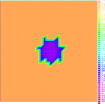
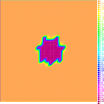
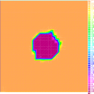
Figure (1) shows the numerical solution of the following diffusive prey-predator system

$$\left\{\begin{array}[]{l}\partial_{t}\rho_{1}-\Delta\rho_{1}-\operatorname*{div}(\rho_{1}\nabla V_{1}[\rho_{1},\rho_{2}])=A\rho_{1}\left(1-\rho_{1}\right)-B\frac{\rho_{1}\rho_{2}}{1+\rho_{1}},\\ \partial_{t}\rho_{2}-\Delta\rho_{2}-\operatorname*{div}(\rho_{2}\nabla V_{2}[\rho_{1},\rho_{2}])=\frac{B\rho_{1}\rho_{2}}{1+\rho_{1}}-C\rho_{2},\end{array}\right..$$

Here the $\rho_{1}$ species are preys and $\rho_{2}$ are predators, see for example [30], the parameters $A=10,C=5,B=70$, and the interactions are chosen as

$$V_{1}[\rho_{1},\rho_{2}]=|x|^{2}\ast\rho_{1}-|x|^{2}\ast\rho_{2},\quad V_{2}[\rho_{1},\rho_{2}]=|x|^{2}\ast\rho_{1}+|x|^{2}\ast\rho_{2}.$$

In (4.4) this corresponds to

$$G_{1}(\rho_{1})=A\frac{\rho_{1}^{2}}{2},\quad G_{2}(\rho_{2})=0,\quad U_{1}[\rho_{1},\rho_{2}]=\frac{B\rho_{2}}{1+\rho_{1}}-A,\quad U_{2}[\rho_{1},\rho_{2}]=-\frac{B\rho_{1}}{1+\rho_{1}}+C.$$

Of course, U1subscript𝑈1U_{1} and U2subscript𝑈2U_{2} satisfy assumptions (4.8) and (4.9), and then Theorem 4.2 gives a solution of the prey-predator system. As before, we shall disregard the uniqueness issue for the sake of simplicity. 
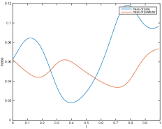
Figure (2) depicts the mass evolution of the prey and predator species: we observe the usual oscillations in time with phase opposition, a characteristic behaviour for Lotka-Volterra types of systems.

$t=0$ $t=0.15$ $t=0.35$ $t=0.5$ $t=0.65$ $t=0.85$ $t=1$
Refer to caption Refer to caption Refer to caption Refer to caption Refer to caption Refer to caption Refer to caption
Figure 1: Evolution of two species with prey-predator interactions. First row: display of $\rho_{1}+\rho_{2}$. Second row: display of the prey $\rho_{1}$. Third row: display of the predator $\rho_{1}$.
Refer to caption
Figure 2: Mass evolution for two-species prey-predator interactions.

5 Application to a tumor growth model with very degenerate enery

In this section we take interest in the equation

$\displaystyle\left\{\begin{array}[]{l}\partial_{t}\rho=\operatorname*{div}(\rho\nabla p)+\rho(1-p),\\ p\geqslant 0\quad\mbox{and}\quad p(1-\rho)=0\\ 0\leqslant\rho\leqslant 1,\\ \rho_{|t=0}=\rho_{0}.\end{array}\right.$ (5.5)

This equation is motivated by tumor growth models [34, 35] and exhibits a Hele-Shaw patch dynamics: if $\rho_{0}=\chi_{\Omega_{0}}$ then the solution remains an indicator $\rho(t)=\chi_{\Omega(t)}$ and the boundary moves with normal velocity $V=-\nabla p|_{\partial\Omega(t)}$, see [2] for a rigorous analysis in the framework of viscosity solutions.

At least formally, we remark that (5.5) is the Wasserstein-Fisher-Rao gradient flow of the singular functional

$$\mathcal{F}(\rho):=\mathcal{F}_{\infty}(\rho)-\int_{\Omega}\rho,$$

where

$$\mathcal{F}_{\infty}(\rho):=\left\{\begin{array}[]{ll}0&\text{ if }\rho\leqslant 1\,\mbox{ a.e},\\ +\infty&\text{ otherwise.}\end{array}\right.$$

Indeed, the compatibility conditions $p\geqslant 0$ and $p(1-\rho)=0$ in (5.5) really mean that the pressure $p$ belongs to the subdifferential $\partial\mathcal{F}_{\infty}(\rho)$, and (5.5) thus reads as the gradient flow

$$\partial_{t}\rho=\operatorname*{div}(\rho\nabla u)-\rho u,\qquad u=p-1\in-\partial\mathcal{F}(\rho).$$

However, this functional is too singular for the previous splitting scheme to correctly capture the very degenerate diffusion. Indeed, the naive and direct approach from section 3 would lead to

$$\left\{\begin{array}[]{l}\rho_{h}^{k+1/2}\in\operatorname*{argmin}\limits_{\rho\leqslant 1,\,|\rho|=|\rho_{h}^{k}|}\left\{\frac{1}{2h}\mathtt{W}^{2}(\rho,\rho_{h}^{k})-\int_{\Omega}\rho\right\},\\ \\ \rho_{h}^{k+1}\in\operatorname*{argmin}\limits_{\rho\leqslant 1}\left\{\frac{1}{2h}\mathtt{FR}^{2}(\rho,\rho_{h}^{k+1/2})-\int_{\Omega}\rho\right\}.\end{array}\right.$$

Since the Wasserstein step is mass-conservative by definition, the $\int\rho$ term has no effect in the first step and the latter reads as “project $\rho_{h}^{k}$ on $\{\rho\leqslant 1\}$ w.r.t to the $\mathtt{W}$ distance”. Since the output of the reaction step $\rho^{k+1}_{h}\leqslant 1$, the Wasserstein step will never actually project anything, and the diffusion is completly shut down. As an example, it is easy to see that if the initial datum is an indicator $\rho_{0}=\chi_{\Omega_{0}}$ then the above naive scheme leads to a stationary solution $\rho^{k+1}_{h}=\rho^{k+1/2}_{h}=\rho_{0}$ for all $k\geqslant 0$, while the real solution should evolve according to the aforementioned Hele-Shaw dynamics $\rho(t)=\chi_{\Omega(t)}$ [2, 34]. One could otherwise try to write a semi-implicit scheme as follows: 1) keep the projection on $\{\rho\leqslant 1\}$ in the first Wasserstein step. As in [29] a pressure term $p^{k+1/2}_{h}$ appears as a Lagrange multiplier in the Wasserstein projection. 2) in the $\mathtt{FR}$/reaction step, relax the constraint $\rho\leqslant 1$ and minimize instead $\rho^{k+1}\in\operatorname*{argmin}\left\{\frac{1}{2h}\mathtt{FR}^{2}(\rho)+\int\rho p^{k+1/2}-\int\rho\right\}$, and keep iterating. This seems to correctly capture the diffusion at least numerically speaking, but raises technical issues in the rigorous proof of convergence and most importantly destroys the variational structure at the discrete level (due to the fact that the reaction step becomes semi-explicit).

We shall use instead an approximation procedure, which preserves the variational structure at the discrete level: it is well-known that the Porous-Medium functional

$$\mathcal{F}_{m}(\rho):=\left\{\begin{array}[]{ll}\int_{\Omega}\frac{\rho^{m}}{m-1}&\text{ if }\rho^{m}\in L^{1}(\Omega)\\ +\infty&\text{ otherwise}\end{array}\right.$$

$\Gamma$-converges to $\mathcal{F}_{\infty}$ as $m\to\infty$, see [7]. In the spirit of [40], one should therefore expect that the gradient flow $\rho_{m}$ of $\mathcal{F}_{m}(\rho)-\int\rho$ converges to the gradient flow $\rho_{\infty}$ of the limiting functional $\mathcal{F}(\rho)=\mathcal{F}_{\infty}(\rho)-\int\rho$. Implementing the splitting scheme for the regular energy functional $\mathcal{F}_{m}(\rho)-\int\rho$ gives a sequence $\rho_{h,m}$, and we shall prove below that $\rho_{h,m}$ converges to a solution of the limiting gradient flow as $m\to\infty$ and $h\to 0$. However, it is known [17] that the limit depends in general on the interplay between the time-step $h$ and the regularization parameter ($m\to\infty$ here), and for technical reasons we shall enforce the condition

$$mh\to 0\qquad\mbox{as }m\to\infty\mbox{ and }h\to 0.$$

Note that [34] already contained a similar approximation $m\to\infty$ but without exploiting the variational structure of the $m$- gradient flow, and our approach is thus different. The above gradient-flow structure was already noticed and fully exploited in the ongoing work [10], where existence and uniqueness of weak solutions is proved and numerical simulations are performed needless of any splitting an using directly the $\mathtt{WFR}$ structure. Here we rather emphasize the fact that the splitting does capture delicate $\Gamma$-convergence phenomena.

In order to make this rigorous, we fix a time step $h>0$ and construct two sequences $(\rho_{h,m}^{k+1/2})_{k}$ and $(\rho_{h,m}^{k})_{k}$, with $\rho_{h,m}^{0}=\rho_{0}$, defined recursively as

$\displaystyle\left\{\begin{array}[]{l}\rho_{h}^{k+1/2}\in\operatorname*{argmin}\limits_{\rho\in\mathcal{M}^{+},\,|\rho|=|\rho_{h}^{k}|}\left\{\frac{1}{2h}\mathtt{W}^{2}(\rho,\rho_{h,m}^{k})+\mathcal{F}_{m}(\rho)-\int_{\Omega}\rho\right\},\\ \\ \rho_{h}^{k+1}\in\operatorname*{argmin}\limits_{\rho\in\mathcal{M}^{+}}\left\{\frac{1}{2h}\mathtt{FR}^{2}(\rho,\rho_{h}^{k+1/2})+\mathcal{F}_{m}(\rho)-\int_{\Omega}\rho\right\}.\end{array}\right.$ (5.9)

As is common in the classical theory of Porous Media Equations [42], we define the pressure as the first variation

$$p_{m}:=F_{m}^{\prime}(\rho)=\frac{m}{m-1}\rho^{m-1}.$$

We accordingly write

$$p_{h,m}^{k+1/2}:=\frac{m}{m-1}(\rho_{h,m}^{k+1/2})^{m-1}\qquad\text{and}\qquad p_{h,m}^{k+1}:=\frac{m}{m-1}(\rho_{h,m}^{k+1})^{m-1}$$

for the discrete pressures. As in section 3 we denote by $\rho_{h,m}(t),p_{h,m}(t)$ and $\tilde{\rho}_{h,m}(t),\tilde{p}_{h,m}(t)$ the piecewise constant interpolations of $\rho_{h,m}^{k+1},p_{h,m}^{k+1}$ and $\rho_{h,m}^{k+1/2},p_{h,m}^{k+1/2}$, respectively.

Our main result is

Theorem 5.1.

Assume that $\rho_{0}\in BV(\Omega)$, $\rho_{0}\leqslant 1$, and $mh\to 0$ as $h\to 0$ and $m\to\infty$. Then for all $T>0$, $\rho_{h,m},\tilde{\rho}_{h,m}$ both converge to some $\rho$ strongly in $L^{1}((0,T)\times\Omega)$, the pressures $p_{h,m},\tilde{p}_{h,m}$ both converge to some $p$ weakly in $L^{2}((0,T),H^{1}(\Omega))$, and $(\rho,p)$ is the unique weak solution of (5.5).

Since we have a $\mathtt{WFR}$ gradient-flow structure, uniqueness should formally follows from the $-1$ geodesic convexity of the driving functional $\mathcal{E}_{\infty}(\rho)-\int_{\Omega}\rho$ with respect to the $\mathtt{WFR}$ distance [24, 26] and the resulting contractivity estimate $\mathtt{WFR}(\rho^{1}(t),\rho^{2}(t))\leq e^{t}\mathtt{WFR}(\rho^{1}_{0},\rho^{2}_{0})$. This is proved rigorously in [10], and therefore we retrieve convergence of the whole sequence $\rho_{h,m}\to\rho$ in Theorem 5.1 (and not only for subsequences). Given this uniqueness, it is clearly enough to prove convergence along any discrete (sub)sequence, and this is exactly what we show below.

The strategy of proof for Theorem 5.1 is exactly as in section 3, except that we need now the estimates to be uniform in both in $h\to 0$ and $m\to\infty$.

5.1 Estimates and convergences

In this section, we improve the previous estimates from section 3. We start with an explicit $L^{\infty}$-bound:

Lemma 5.2.

Assume that $\rho_{0}\leqslant 1$, then for all $t\in\operatorname*{\mathbb{R}}^{+}$,

$$\|\rho_{h,m}(t,\cdot)\|_{\infty},\|\tilde{\rho}_{h,m}(t,\cdot)\|_{\infty}\leqslant 1.$$
Démonstration.

We argue by induction at the discrete level, starting from $\rho_{0}=\rho^{0}_{h,m}\leqslant 1$ by assumption. If $\|\rho_{h,m}^{k}\|_{\infty}\leqslant 1$, Otto’s maximum principle [31] implies that $\|\rho_{h,m}^{k+1/2}\|_{\infty}\leqslant\|\rho_{h,m}^{k}\|_{\infty}\leqslant 1$ in the Wasserstein step.

Assume now by contradiction that $E:=\{\rho_{h,m}^{k+1}>1\}$ has positive Lebesgue measure. The optimality condition (3.17) for the Fisher-Rao minimization step gives, dividing by $\sqrt{\rho_{h,m}^{k+1}}>0$ in $E$,

$$\sqrt{\rho_{h,m}^{k+1}}-\sqrt{\rho_{h,m}^{k+1/2}}=\frac{h}{2}\sqrt{\rho_{h,m}^{k+1}}\left(1-\frac{m}{m-1}(\rho_{h,m}^{k+1})^{m-1}\right)$$

Then $1-\frac{m}{m-1}(\rho_{h,m}^{k+1})^{m-1}\leqslant 1-\frac{m}{m-1}<0$ in the right-hand side, hence the desired contradiction $\rho_{h,m}^{k+1}<\rho_{h,m}^{k+1/2}\leqslant 1$. ∎

Noticing that the functional $\frac{1}{m-1}\int\rho^{m}-\int\rho$ corresponds to taking explicitly $F_{2}(z)=z^{m}/m-1$ and $V_{2}(x)\equiv-1$ in section 3, it is easy to reproduce the computations from the proof of Lemma 3.5 and carefully track the dependence of the constants w.r.t $m>1$ to obtain

Lemma 5.3.

There exists $c>0$ such that, for all $m>m_{0}$ large enough and all $h\leq h_{0}$ small enough,

$$(1-ch)\rho^{k+1/2}_{h,m}(x)\leqslant\rho^{k+1}_{h,m}(x)\leqslant(1+h)\rho^{k+1/2}_{h,m}(x)\qquad\mbox{a.e.}$$ (5.10)

Note that this holds regardless of any compatibility such as $hm\to 0$. The key point is here that the lower bound $c$ previously depended on an upper bound $M$ on $\rho^{k+1/2}$ in Lemma 3.5, but since we just obtained in Lemma 5.2 the universal upper bound $\rho^{k+1/2}\leqslant 1$ we end up with a lower bound which is also uniform in $h,m$. The proof is identical to that of Lemma 3.5 and we omit the details for simplicity.

Recalling that the Wasserstein step is mass-preserving, we obtain by immediate induction and for all $0\leq t\leq T$

$$\|\rho_{h,m}(t)\|_{L^{1}},\,\|\tilde{\rho}_{h,m}(t)\|_{L^{1}}\leqslant e^{T}\|\rho_{0}\|_{L^{1}}$$

as well as

$$\|\rho_{h,m}(t)-\tilde{\rho}_{h,m}(t)\|_{L^{1}}\leqslant C_{T}h.$$ (5.11)

Testing successively $\rho=\rho_{h,m}^{k}$ and $\rho=\rho_{h,m}^{k+1/2}$ in (5.9), we get

$$\frac{1}{2h}\left(\mathtt{W}^{2}(\rho_{h,m}^{k},\rho_{h,m}^{k+1/2})+\mathtt{FR}^{2}(\rho_{h,m}^{k+1/2},\rho_{h,m}^{k+1})\right)\leqslant\mathcal{F}_{m}(\rho_{h,m}^{k})-\mathcal{F}_{m}(\rho_{h,m}^{k+1})+\int_{\Omega}(\rho_{h,m}^{k+1/2}-\rho_{h,m}^{k+1}).$$

Using Proposition 2.4 to control $\mathtt{WFR}^{2}\lesssim 2(\mathtt{W}^{2}+\mathtt{FR}^{2})$ and the lower bound in (5.10) yields

$\displaystyle\frac{1}{4h}\mathtt{WFR}^{2}(\rho^{k+1}_{h,m},\rho^{k}_{h,m})$ $\displaystyle\leqslant$ $\displaystyle\frac{1}{2h}\left(\mathtt{W}^{2}(\rho_{h,m}^{k},\rho_{h,m}^{k+1/2})+\mathtt{FR}^{2}(\rho_{h,m}^{k+1/2},\rho_{h,m}^{k+1})\right)$
$\displaystyle\leqslant$ $\displaystyle\mathcal{F}_{m}(\rho_{h,m}^{k})-\mathcal{F}_{m}(\rho_{h,m}^{k+1})+\int_{\Omega}(\rho_{h,m}^{k+1/2}-\rho_{h,m}^{k+1})$
$\displaystyle\leqslant$ $\displaystyle\mathcal{F}_{m}(\rho_{h,m}^{k})-\mathcal{F}_{m}(\rho_{h,m}^{k+1})+ch\int_{\Omega}\rho_{h,m}^{k+1/2}$
$\displaystyle\leqslant$ $\displaystyle\mathcal{F}_{m}(\rho_{h,m}^{k})-\mathcal{F}_{m}(\rho_{h,m}^{k+1})+che^{T}$

for all $k\leqslant N:=\lfloor T/h\rfloor$.

Summing over $k$ we get

$\displaystyle\frac{1}{4h}\sum_{k=0}^{N-1}\mathtt{WFR}^{2}(\rho_{h,m}^{k},\rho_{h,m}^{k+1})$ $\displaystyle\leqslant$ $\displaystyle\mathcal{F}_{m}(\rho_{0})-\mathcal{F}_{m}(\rho_{h,m}^{N})+C_{T}$
$\displaystyle\leqslant$ $\displaystyle\frac{1}{m-1}\int_{\Omega}\rho_{0}^{m}+C_{T}\leqslant\frac{1}{m-1}\int_{\Omega}\rho_{0}+C_{T}\leqslant C_{T},$

where we used successively $F_{m}\geq 0$ to get rid of $\mathcal{F}_{m}(\rho^{N}_{h,m})$, and $\rho_{0}^{m}\leq\rho_{0}$ for $\rho_{0}\leq 1$ and $m>1$.

Consequently, for all fixed $T>0$ and any $t,s\in[0,T]$ we obtain the classical $\frac{1}{2}$-Hölder estimate

$\displaystyle\left\{\begin{array}[]{l}\mathtt{WFR}(\rho_{h,m}(t),\rho_{h,m}(s))\leqslant C_{T}|t-s+h|^{1/2},\\ \mathtt{WFR}(\tilde{\rho}_{h,m}(t),\tilde{\rho}_{h,m}(s))\leqslant C_{T}|t-s+h|^{1/2}.\end{array}\right.$ (5.14)

Exploiting the explicit algebraic structure of $F_{m}(z)=\frac{1}{m-1}z^{m}$, compactness in space will be given here by

Lemma 5.4.

If $\rho_{0}\in BV(\Omega)$ then

$$\sup_{t\in[0,T]}\left\{\|\rho_{h,m}(t,\cdot)\|_{BV(\Omega)},\|\tilde{\rho}_{h,m}(t,\cdot)\|_{BV(\Omega)}\right\}\leqslant e^{T}\|\rho_{0}\|_{BV(\Omega)}.$$
Démonstration.

The argument closely follows the lines of [18, prop. 5.1]. We first note from [14, thm. 1.1] that the $BV$-norm is nonincreasing during the Wasserstein step,

$$\|\rho_{h,m}^{k+1/2}\|_{BV(\Omega)}\leqslant\|\rho_{h,m}^{k}\|_{BV(\Omega)}.$$

Using as before the implicit function theorem, we show below that $\rho_{h,m}^{k+1}=R(\rho_{h,m}^{k+1/2})$ for some suitable $(1+h)$-Lispchitz function $R$. By standard $Lip\circ BV$ composition [3] this will prove that

$$\|\rho_{h,m}^{k+1}\|_{BV(\Omega)}\leqslant(1+h)\|\rho_{h,m}^{k+1/2}\|_{BV(\Omega)}$$

and will conclude the proof by immediate induction.

Indeed, we already know from (5.10) that $\rho_{h,m}^{k+1/2}$ and $\rho_{h,m}^{k+1}$ share the same support. In this support and from (3.17) it is easy to see that $\rho=\rho_{h,m}^{k+1}(x)$ is the unique positive solution of $f(\rho,\rho_{h,m}^{k+1/2}(x))=0$ with

$$f(\rho,\mu)=\sqrt{\rho}\left(1-\frac{h}{2}\left(1-\frac{m}{m-1}\rho^{m-1}\right)\right)-\sqrt{\mu}.$$

For $\mu>0$, the implicit function theorem gives the existence of a $\mathcal{C}^{1}$ map $R$ such that $f(\rho,\mu)=0\Leftrightarrow\rho=R(\mu)$, with $R(0)=0$. An algebraic computation shows moreover that $0<\frac{dR}{d\mu}=-{\frac{\partial_{\mu}f}{\partial_{\rho}f}}_{|\rho=R(\mu)}\leqslant(1+h)$ uniformly in $m>1$, hence $R$ is $(1+h)$-Lipschitz as claimed and the proof is complete.

Proposition 5.5.

Up to extraction of a discrete sequence $h\to 0,m\to\infty$, there holds

$$\rho_{h,m},\,\tilde{\rho}_{h,m}\to\rho\qquad\mbox{strongly in }L^{1}(Q_{T})$$
$$p_{h,m}\rightharpoonup p\quad\mbox{and}\quad\tilde{p}_{h,m}\rightharpoonup\tilde{p}\qquad\mbox{weakly in all }L^{q}(Q_{T})$$

for all $T>0$. If in addition $mh\to 0$ then $p=\tilde{p}$.

Démonstration.

The first part of the statement follows exactly as in section 3, exploiting the $\frac{1}{2}$-Hölder estimates (5.14) and the space compactness from Proposition 5.4 in order to apply the Rossi-Savaré theorem [39]. The fact that $\rho_{h,m},\tilde{\rho}_{h,m}$ have the same limit comes from (5.11).

For the pressures, we simply note from $\rho_{h,m}\leqslant 1$ and $m\gg 1$ that $p_{h,m}=\frac{m}{m-1}\rho_{h,m}^{m-1}\leqslant 2\rho_{h,m}$ is bounded in $L^{1}\cap L^{\infty}(Q_{T})$ uniformly in $h,m$ in any finite time interval $[0,T]$. Thus up to extraction of a further sequence we have $p_{h,m}\rightharpoonup p$ in all $L^{q}(Q_{T})$, and likewise for $\tilde{p}_{h,m}\rightharpoonup\tilde{p}$.

Finally, we only have to check that $p=\tilde{p}$ if $hm\to 0$. Because $\rho_{h,m},\tilde{\rho}_{h,m}\leqslant 1$ and $z\mapsto z^{m-1}$ is $(m-1)$-Lipschitz on $[0,1]$ we have for all fixed $t\geqslant 0$ that

$\displaystyle\int_{\Omega}|p_{m,h}(t,\cdot)-\tilde{p}_{m,h}(t,\cdot)|$ $\displaystyle=$ $\displaystyle\int_{\Omega}\frac{m}{m-1}|\rho_{h,m}^{m-1}(t,\cdot)-\tilde{\rho}_{h,m}^{m-1}(t,\cdot)|$
$\displaystyle\leqslant$ $\displaystyle m\int_{\Omega}|{\rho_{h,m}(t)}-{\tilde{\rho}_{h}(t)}|\leqslant C_{T}hm\longrightarrow 0,$

where we used (5.11) in the last inequality. Hence $p=\tilde{p}$ and the proof is complete.

In order to pass to the limit in the diffusion term $\operatorname*{div}(\rho\nabla p)$ we first improve the convergence of $\tilde{p}_{h,m}$:

Lemma 5.6.

There exists a constant $C_{T}$, independent of $h$ and $m$, such that

$$\|\tilde{p}_{h,m}\|_{L^{2}((0,T),H^{1}(\Omega))}\leqslant C_{T}$$

for all $T>0$. Consequently, up to a subsequence, $\tilde{p}_{h,m}$ converges weakly in $L^{2}((0,T),H^{1}(\Omega))$ to $p$.

Démonstration.

The proof is based on the flow interchange technique developed by Matthes, McCann and Savaré in [28]. Let $\eta$ be the (smooth) solution of

$$\left\{\begin{array}[]{l}\partial_{t}\eta=\Delta\eta^{m-1}+\varepsilon\Delta\eta,\\ \eta|_{t=0}=\rho^{k+1/2}_{h,m}.\end{array}\right.$$

It is well known [4] that $\eta$ is the Wasserstein gradient flow of

$$\mathcal{G}(\rho):=\int_{\Omega}\frac{\rho^{m-1}}{m-2}+\varepsilon\int_{\Omega}\rho\log(\rho).$$

Since $\mathcal{G}$ is geodesically 00-convex, $\eta$ satisfies the Evolution Variational Inequality (EVI)

$$\left.\frac{1}{2}{\frac{d^{+}}{dt}}\right|_{t=s}\mathtt{W}^{2}(\eta(s),\rho)\leqslant\mathcal{G}(\rho)-\mathcal{G}(\eta(s)),$$

for all $s>0$ and for all $\rho\in\operatorname*{\mathcal{P}^{ac}}(\Omega)$, where $\frac{d^{+}}{dt}f(t):=\limsup\limits_{s\rightarrow 0^{+}}\frac{f(t+s)-f(t)}{s}$. By optimality of $\rho^{k+1/2}_{h,m}$ in (5.9), we obtain that

$$\left.\frac{1}{2}{\frac{d^{+}}{dt}}\right|_{t=s}\mathtt{W}^{2}(\eta(s),\rho_{h,m}^{k})\geqslant-h\left.{\frac{d^{+}}{dt}}\right|_{t=s}\mathcal{F}_{m}(\eta(s)).$$

Since $\eta$ is smooth due to the regularizing $\varepsilon\Delta$ term, we can legitimately integrate by parts for all $s>0$

$\displaystyle\frac{d}{ds}\mathcal{F}_{m}(\eta(s))$ $\displaystyle=$ $\displaystyle\int_{\Omega}\frac{m}{m-1}\eta(s)^{m-1}(\Delta\eta(s)^{m-1}+\varepsilon\Delta\eta(s))$
$\displaystyle=$ $\displaystyle-\int_{\Omega}\frac{m}{m-1}|\nabla\eta(s)^{m-1}|^{2}-\varepsilon\int_{\Omega}m\eta(s)^{m-2}|\nabla\eta(s)|^{2}$
$\displaystyle\leqslant$ $\displaystyle-\int_{\Omega}\frac{m}{m-1}|\nabla\eta(s)^{m-1}|^{2}=-\frac{m-1}{m}\int_{\Omega}\left|\nabla\left(\frac{m}{m-1}\eta(s)^{m-1}\right)\right|^{2}$

Remarking that $\frac{m}{m-1}\eta(s)^{m-1}\to\frac{m}{m-2}\rho_{h,m}^{k+1/2}=p_{h,m}^{k+1/2}$ as $s\to 0$, an easy lower semi-continuity argument gives that

$$\int_{\Omega}\frac{m-1}{m}|\nabla p_{h,m}^{k+1/2}|^{2}=\int_{\Omega}\frac{m}{m-1}|\nabla(\rho_{h,m}^{k+1/2})^{m-1}|^{2}\leqslant\liminf_{s\searrow 0}\left.{\frac{d^{+}}{dt}}\right|_{t=s}\mathcal{F}_{m}(\eta(s)).$$

Then we have

$\displaystyle h\int_{\Omega}\frac{m-1}{m}|\nabla p_{h,m}^{k+1/2}|^{2}$ $\displaystyle\leqslant\mathcal{F}_{m-1}(\rho_{h,m}^{k})-\mathcal{F}_{m-1}(\rho_{h,m}^{k+1/2})$
$\displaystyle+\varepsilon\left(\int_{\Omega}\rho_{h,m}^{k}\log(\rho_{h,m}^{k})-\int_{\Omega}\rho_{h,m}^{k+1/2}\log(\rho_{h,m}^{k+1/2})\right).$

First arguing as in Proposition 3.7 to control

$$\mathcal{F}_{m-1}(\rho_{h,m}^{k+1})\leqslant\mathcal{F}_{m-1}(\rho_{h,m}^{k+1/2})+C_{T}h,$$

and then passing to the limit $\varepsilon\searrow 0$, we obtain

$$h\int_{\Omega}\frac{m-1}{m}|\nabla p_{h,m}^{k+1/2}|^{2}\leqslant\mathcal{F}_{m-1}(\rho_{h,m}^{k})-\mathcal{F}_{m-1}(\rho_{h,m}^{k+1})+C_{T}h.$$

Summing over $k$ gives

$$\int_{0}^{T}\int_{\Omega}|\nabla\tilde{p}_{h,m}(t,x)|^{2}\,dxdt\leqslant\frac{m}{m-1}(\mathcal{F}_{m-1}(\rho_{0})-\mathcal{F}_{m-1}(\rho^{N}_{h,m})+C_{T})\leqslant 2\mathcal{F}_{m-1}(\rho_{0})+C_{T}$$

for all $T<+\infty$. Due to $\rho_{0}\leqslant 1$ and $m\gg 1$ we can bound $\mathcal{F}_{m-1}(\rho_{0})=\frac{1}{m-2}\int\rho_{0}^{m-1}\leqslant\frac{1}{m-2}\int\rho_{0}\leqslant\|\rho_{0}\|_{L^{1}(\Omega)}$ and the result finally follows. ∎

5.2 Properties of the pressure $p$ and conclusion

We start by showing that the limits $\rho,p$ satisfy the compatibility conditions in (5.5).

Lemma 5.7.

There holds

$$0\leqslant\rho,p\leqslant 1\quad\text{and}\quad p(1-\rho)=0\,\text{ a.e. in }Q_{T}.$$
Démonstration.

By Lemma 5.2 it is obvious that $0\leqslant\rho\leqslant 1$ and $0\leqslant p\leqslant 1$ are inherited from $0\leqslant\rho_{h,m}\leqslant 1$ and $0\leqslant p_{h,m}=\frac{m}{m-1}\rho^{m-1}_{h,m}\leqslant\frac{m}{m-1}$.

In order to prove that $p(1-\rho)=0$, we first observe that

$$p_{h,m}(1-\rho_{h,m})\to 0\qquad\mbox{a.e. in }Q_{T}.$$

Indeed, since $\rho_{h,m}\to\rho$ strongly in $L^{1}(Q_{T})$ we have $\rho_{h,m}(t,x)\to\rho(t,x)$ a.e. If the limit $\rho(t,x)<1$ then $\rho_{h,m}(t,x)\leqslant(1-\varepsilon)$ for small $h$ and large $m$. Hence $p_{h,m}(t,x)=\frac{m}{m-1}\rho_{h,m}^{m-1}\leqslant\frac{m}{m-1}(1-\varepsilon)^{m-1}\to 0$ while $1-\rho_{h,m}$ remains bounded, and therefore the product $p_{h,m}(1-\rho_{h,m})\to 0$. Now if the limit $\rho(t,x)=1$ then the pressure $p_{h,m}=\frac{m}{m-1}\rho_{h,m}^{m-1}\leqslant\frac{m}{m-1}$ remains bounded, while $1-\rho_{h,m}(t,x)\to 0$ hence the product goes to zero in this case too.

Thanks to the uniform $L^{\infty}$ bounds $\rho_{h,m}\leqslant 1$ and $p_{h,m}\leqslant\frac{m}{m-1}\leqslant 2$ we can apply Lebesgue’s convergence theorem to deduce from this pointwise a.e. convergence that, for all fixed nonnegative $\varphi\in\mathcal{\mathcal{missing}}C^{\infty}_{c}(Q_{T})$, there holds

$$\lim\int_{Q_{T}}p_{h,m}(1-\rho_{h,m})\varphi=0.$$

On the other hand since $\rho_{h,m}\to\rho$ strongly in $L^{1}(Q_{T})$ hence a.e, and because $0\leqslant\rho_{h,m}\leqslant 1$, we see that $(1-\rho_{h,m})\varphi\to(1-\rho)\varphi$ in all $L^{q}(Q_{T})$. From Proposition 5.5 we also had that $p_{h,m}\rightharpoonup p$ in all $L^{q}(Q_{T})$, hence by strong-weak convergence we have that

$$\int_{Q_{T}}p(1-\rho)\varphi=\lim\int_{Q_{T}}p_{h,m}(1-\rho_{h,m})\varphi=0$$

for all $\varphi\geqslant 0$. Because $p(1-\rho)\geqslant 0$ we conclude that $p(1-\rho)=0$ a.e. in $Q_{T}$ and the proof is achieved.

We end this section with

Proof of Theorem 5.1.

We only sketch the argument and refer to [18] for the details. Fix any $0<t_{1}<t_{2}$ and $\varphi\in\mathcal{C}^{2}_{c}(\operatorname*{\mathbb{R}}^{d})$. Exploiting the Euler-Lagrange equations (3.14)(3.17) and summing from $k=k_{1}=\lfloor t_{1}/h\rfloor$ to $k=k_{2}-1=\lfloor t_{2}/h\rfloor-1$, we first obtain

$$\int_{\operatorname*{\mathbb{R}}^{d}}\rho_{h,m}(t_{2})\varphi-\rho_{h,m}(t_{1})\varphi+\int_{k_{1}h}^{k_{2}h}\int_{\operatorname*{\mathbb{R}}^{d}}\tilde{\rho}_{h,m}\nabla\tilde{p}_{h,m}\cdot\nabla\varphi=-\int_{k_{1}h}^{k_{2}h}\int_{\operatorname*{\mathbb{R}}^{d}}\rho_{h,m}(1-p_{h,m})\varphi+R(h,m),$$

where the remainder $R(h,m)\to 0$ for fixed $\varphi$. The strong convergence $\rho_{h,m},\tilde{\rho}_{h,m}\to\rho$ and the weak convergences $\nabla\tilde{p}_{h,m}\rightharpoonup\nabla\tilde{p}=\nabla p$ and $p_{h,m}\rightharpoonup p$ are then enough pass to the limit to get the corresponding weak formulation for all $0<t_{1}<t_{2}$. Moreover since the limit $\rho\in\mathcal{C}([0,T];\mathcal{M}^{+}_{\mathtt{WFR}})$ the initial datum $\rho(0)=\rho_{0}$ is taken at least in the sense of measures. This gives an admissible weak formulation of (5.5), and the proof is complete. ∎

5.3 Numerical simulation

The constructive scheme (5.9) naturally leads to a fully discrete algorithm, simply discretizing the minimization problem in space for each $\mathtt{W},\mathtt{FR}$ step. We use again the ALG2-JKO scheme [6] for the Wasserstein steps. As already mentioned the Fisher-Rao step is a mere convex pointwise minimization problem, here explicitly given by: for all $x\in\Omega$,

$$\rho_{h,m}^{k+1}(x)=\operatorname*{argmin}_{\rho\geq 0}\left\{4\left|\sqrt{\rho}-\sqrt{\rho_{h,m}^{k+1/2}(x)}\right|^{2}+2h\left(\frac{\rho^{m}}{m-1}-1\right)\right\}$$

and poses no difficulty in the practical implementation using a standard Newton method.

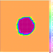
Figure 3 depicts the evolution of the numerical solution $\rho_{h,m}$ for $m=100$ and with a time step $h=0.005$. We remark that the tumor first saturates the constraint ($\rho\nearrow 1$) in its initial support, and then starts diffusing outwards. This is consistent with the qualitative behaviour described in [34].

Refer to caption Refer to caption Refer to caption Refer to caption Refer to caption
$t=0$ $t=0.3$ $t=0.5$ $t=0.7$ $t=1$
Figure 3: Snapshot of the approximate solution $\rho_{h,m}(t,.)$ to (5.5), with $m=100$, $h=0.005$.

6 A tumor growth model with nutrient

In this section we use the same approach for the following tumor growth model with nutrients, appearing e.g. in [34]

$\displaystyle\left\{\begin{array}[]{l}\partial_{t}\rho-\operatorname*{div}(\rho\nabla p)=\rho\left((1-p)(c+c_{1})-c_{2}\right),\\ \partial_{t}c-\Delta c=-\rho c,\\ 0\leqslant\rho\leqslant 1,\\ p\geqslant 0\mbox{ and }p(1-\rho)=0,\\ \rho_{|t=0}=\rho_{0},\,c_{|t=0}=c_{0}.\end{array}\right.$ (6.6)

Here $c_{1}$ and $c_{2}$ are two positive constants, and the nutrient $c$ is now diffusing in $\Omega$ in addition to begin simply consumed by the tumor $\rho$, according to the second equation. For technical convenience we work here on a convex bounded domain $\Omega\subset\mathbb{R}^{d}$, endowed with natural Neumann boundary conditions for both $\rho$ and $c$.

Contrarily to section 5 this is not a $\mathtt{WFR}$ gradient flow anymore, and we therefore introduce a semi-implicit splitting scheme. Starting from the initial datum $\rho^{0}_{h,m}:=\rho_{0},c_{h,m}^{0}:=c_{0}$ we construct four sequences $\rho_{h,m}^{k+1/2},\rho_{h,m}^{k},c_{h,m}^{k+1/2},c_{h,m}^{k}$, defined recursively as

$\displaystyle\left\{\begin{array}[]{l}\rho_{h,m}^{k+1/2}\in\operatorname*{argmin}\limits_{\rho\in\mathcal{M}^{+},|\rho|=|\rho_{h,m}^{k}|}\left\{\frac{1}{2h}\mathtt{W}^{2}(\rho,\rho_{h,m}^{k})+\mathcal{F}_{m}(\rho)\right\},\\ \\ c_{h,m}^{k+1/2}\in\operatorname*{argmin}\limits_{c\in\mathcal{M}^{+},|c|=|c_{h,m}^{k}|}\left\{\frac{1}{2h}\mathtt{W}^{2}(c,c_{h,m}^{k})+\mathcal{E}(\rho)\right\},\end{array}\right.$ (6.10)

and

$\displaystyle\left\{\begin{array}[]{l}\rho_{h,m}^{k+1}\in\operatorname*{argmin}\limits_{\rho\in\mathcal{M}^{+}}\left\{\frac{1}{2h}\mathtt{FR}^{2}(\rho,\rho_{h,m}^{k+1/2})+\mathcal{E}_{1,m}(\rho|c_{h,m}^{k+1/2})\right\},\\ \\ c_{h,m}^{k+1}\in\operatorname*{argmin}\limits_{c\in\mathcal{M}^{+}}\left\{\frac{1}{2h}\mathtt{FR}^{2}(c,c_{h,m}^{k+1/2})+\mathcal{E}_{2}(c|\rho_{h,m}^{k+1/2})\right\},\par\end{array}\right.$ (6.14)

where

$$\mathcal{E}(\rho):=\int_{\Omega}\rho\log(\rho),$$
$$\mathcal{E}_{1,m}(\rho|c):=\int_{\Omega}\left(c+c_{1}\right)\frac{\rho^{m}}{m-1}+\int_{\Omega}(c_{2}-c-c_{1})\rho,$$

and

$$\mathcal{E}_{2}(c|\rho):=\int_{\Omega}\rho c.$$

As earlier it is easy to see that these sequences are well-defined (i-e there exists a unique minimizer for each step), and the pressures are defined as before as

$$p_{h,m}^{k+1/2}:=\frac{m}{m-1}(\rho_{h,m}^{k+1/2})^{m-1}\quad\mbox{and}\quad p_{h,m}^{k+1}:=\frac{m}{m-1}(\rho_{h,m}^{k+1})^{m-1}.$$

We denote again by $a_{h,m}(t),\tilde{a}_{h,m}(t)$ the piecewise constant interpolation of any discrete quantity $a^{k+1}_{h,m},a^{k+1/2}_{h,m}$ respectively. Our main result reads:

Theorem 6.1.

Assume $\rho_{0}\in BV(\Omega)$ with $\rho_{0}\leqslant 1$ and $c_{0}\in L^{\infty}(\Omega)\cap BV(\Omega)$. Then $\rho_{h,m}$ and $\tilde{\rho}_{h,m}$ strongly converge to $\rho$ in $L^{1}((0,T)\times\Omega)$ and $c_{h,m}$ and $\tilde{c}_{h,m}$ strongly converge to $c$ in $L^{1}((0,T)\times\Omega)$ when $h\searrow 0$ and $m\nearrow+\infty$. Moreover, if $mh\rightarrow 0$, then $p_{h,m},\tilde{p}_{h,m}$ converge weakly in $L^{2}((0,T),H^{1}(\Omega))$ to a unique $p$, and $(\rho,p,c)$ is a solution of (6.6).

Note that uniqueness of solutions would result in convergence of the whole sequence. Uniqueness was proved in [34, thm. 4.2] for slightly more regular weak solutions, but we did not push in this direction for the sake of simplicity. The method of proof is almost identical to section 5 so we only sketch the argument and emphasize the main differences.

We start by recalling the optimality conditions for the scheme (6.10)-(6.14). The Euler-Lagrange equations for the tumor densities in the Wasserstein and Fisher-Rao steps are

$\displaystyle\left\{\begin{array}[]{l}\rho_{h,m}^{k+1/2}\nabla p_{h,m}^{k+1/2}=\frac{\nabla\varphi}{h}\rho_{h,m}^{k+1/2},\\ \sqrt{\rho_{h,m}^{k+1}}-\sqrt{\rho_{h,m}^{k+1/2}}=\frac{h}{2}\sqrt{\rho_{h,m}^{k+1}}\left((1-p_{h,m}^{k+1})(c_{h,m}^{k+1/2}+c_{1})-c_{2}\right),\end{array}\right.$ (6.17)

where $\varphi$ is a (backward) Kantorovich potential for $\mathtt{W}(\rho_{h,m}^{k+1/2},\rho_{h,m}^{k})$. For the nutrient, the Euler-Lagrange equations are

$\displaystyle\left\{\begin{array}[]{l}\nabla c_{h,m}^{k+1/2}=\frac{\nabla\psi}{h}c_{h,m}^{k+1/2},\\ \sqrt{c_{h,m}^{k+1}}-\sqrt{c_{h,m}^{k+1/2}}=-\frac{h}{2}\sqrt{c_{h,m}^{k+1}}\rho_{h,m}^{k+1/2},\end{array}\right.$ (6.20)

with $\psi$ a Kantorovich potential for $\mathtt{W}(c_{h,m}^{k+1/2},c_{h,m}^{k})$.

Using the optimality conditions for the Fischer-Rao steps, we obtain directly the following $L^{\infty}$ bounds:

Lemma 6.2.

For all $k\geqslant 0$

$$\|c_{h,m}^{k+1}\|_{L^{\infty}(\Omega)}\leqslant\|c_{h,m}^{k+1/2}\|_{L^{\infty}(\Omega)}\leqslant\|c_{h,m}^{k}\|_{L^{\infty}(\Omega)},$$

and at the continuous level

$$\|c_{h,m}(t,\cdot)\|_{L^{\infty}(\Omega)},\|\tilde{c}_{h,m}(t,\cdot)\|_{L^{\infty}(\Omega)}\leqslant\|c_{0}\|_{L^{\infty}(\Omega)}\qquad\forall\,t\geq 0.$$

Moreover,

$$\|\rho_{h,m}(t,\cdot)\|_{\infty},\|\tilde{\rho}_{h,m}(t,\cdot)\|_{\infty}\leqslant 1$$

and there exists $c_{T}\equiv c_{T}(\|c_{0}\|_{L^{\infty}}),C_{T}\equiv C_{T}(\|c_{0}\|_{L^{\infty}})>0$ such that

$$\begin{array}[]{c}(1-c_{T}h)\rho_{h,m}^{k+1/2}(x)\leqslant\rho_{h,m}^{k+1}(x)\leqslant(1+C_{T}h)\rho_{h,m}^{k+1/2}(x)\qquad\mbox{a.e. in }\Omega.\\ (1-h)c_{h,m}^{k+1/2}(x)\leqslant c_{h,m}^{k+1}(x)\leqslant c_{h,m}^{k+1/2}(x)\qquad\mbox{a.e. in }\Omega.\end{array}$$ (6.21)
Démonstration.

The proof of the estimates on $c_{h,m}$ and $\tilde{c}_{h,m}$ is obvious because one step of Wasserstein gradient flow with the Boltzmann entropy decreases the $L^{\infty}$-norm in (6.10) (see [32, 1]), and, because the product $\sqrt{c_{h,m}^{k+1}}\rho_{h,m}^{k+1/2}$ is nonnegative in (6.20), the $L^{\infty}$-norm is also nonincreasing during the Fischer-Rao step. The proof for $\rho_{h,m}$ and $\tilde{\rho}_{h,m}$ is the same as in lemma 5.2. Using the fact that $\|\tilde{\rho}_{h,m}(t,\cdot)\|_{\infty}\leqslant 1$, we see that the term $\Phi(p_{h,m}^{k+1},c_{h,m}^{k+1/2}):=(1-p_{h,m}^{k+1})(c_{h,m}^{k+1/2}+c_{1})-c_{2}$ in (6.17) is bounded in $L^{\infty}$ uniformly in $k$. This allows to argue exactly as in Lemma 3.5 to retrieve the estimate (6.21) and concludes the proof. ∎

With these bounds it is easy to prove as in proposition 3.23 that

$$\begin{array}[]{c}\mathcal{F}_{m}(\rho_{h,m}^{k+1})\leqslant\mathcal{F}_{m}(\rho_{h,m}^{k+1/2})+C_{T}h,\\ \mathcal{E}_{1,m}(\rho_{h,m}^{k+1/2}|c_{h,m}^{k+1/2})-\mathcal{E}_{1,m}(\rho_{h,m}^{k+1}|c_{h,m}^{k+1/2})\leqslant C_{T}h,\\ \mathcal{E}(c_{h,m}^{k+1})\leqslant\mathcal{E}(c_{h,m}^{k+1/2})+C_{T}h,\\ \mathcal{E}_{2}(c_{h,m}^{k+1/2}|\rho_{h,m}^{k+1/2})-\mathcal{E}_{2}(c_{h,m}^{k+1}|\rho_{h,m}^{k+1/2})\leqslant C_{T}h,\end{array}.$$

for some $C_{T}$ independent of $m$. Then we obtain the usual $\frac{1}{2}$-Hölder estimates in time with respect to the $\mathtt{WFR}$ distance, which in turn implies that $\rho_{h,m},\tilde{\rho}_{h,m}$ converge to some $\rho\in L^{\infty}([0,T],L^{1}(\Omega))$ and $c_{h,m},\tilde{c}_{h,m}$ converge to some $c\in L^{\infty}([0,T],L^{1}(\Omega))$ pointwise in time with respect to $\mathtt{WFR}$, see (3.28), Proposition 3.8, and (3.30) for details.

As before we need to improve the convergence in order to pass to the limit in the nonlinear terms. For $\rho_{h,m}$ and $\tilde{\rho}_{h,m}$, this follows from

Lemma 6.3.

For all $T>0$, if $\rho_{0},c_{0}\in BV(\Omega)$,

$$\begin{array}[]{c}\sup\limits_{t\in[0,T]}\left\{\|\rho_{h,m}(t,\cdot)\|_{BV(\Omega)}+\|c_{h,m}(t,\cdot)\|_{BV(\Omega)}\right\}\leqslant e^{C_{T}T}(\|\rho_{0}\|_{BV(\Omega)}+\|c_{0}\|_{BV(\Omega)})\\ \sup\limits_{t\in[0,T]}\left\{\|\tilde{\rho}_{h,m}(t,\cdot)\|_{BV(\Omega)}+\|\tilde{c}_{h,m}(t,\cdot)\|_{BV(\Omega)}\right\}\leqslant e^{C_{T}T}(\|\rho_{0}\|_{BV(\Omega)}+\|c_{0}\|_{BV(\Omega)}).\end{array}$$
Démonstration.

The argument is a generalization of Lemma 5.4, see [18, remark 5.1]. First, the $BV$-norm is nonincreasing during the Wasserstein step, [14, thm. 1.1],

$$\|\rho_{h,m}^{k+1/2}\|_{BV(\Omega)}\leqslant\|\rho_{h,m}^{k}\|_{BV(\Omega)}\text{ and }\|c_{h,m}^{k+1/2}\|_{BV(\Omega)}\leqslant\|c_{h,m}^{k}\|_{BV(\Omega)}.$$

Arguing as in Lemma 5.4, we observe that, inside $\mathop{\rm supp}\rho_{h,m}^{k+1/2}=\mathop{\rm supp}\rho_{h,m}^{k+1}$, the minimizer $\rho=\rho_{h,m}^{k+1}(x)$ is the unique positive solution of $f(\rho,\rho_{h,m}^{k+1/2}(x),c_{h,m}^{k+1/2}(x))=0$, with

$$f(\rho,\mu,c)=\sqrt{\rho}\left(1-\frac{h}{2}\left(\left(1-\frac{m}{m-1}\rho^{m-1}\right)(c+c_{1})-c_{2}\right)\right)-\sqrt{\mu}.$$

For $\mu>0$ the implicit function theorem gives as before a $\mathcal{C}^{1}$ map $R$ such that $f(\rho,\mu,c)=0\Leftrightarrow\rho=R(\mu,c)$. An easy algebraic computation and (6.21) then gives $0<\partial_{\mu}R(\mu,c)\leqslant(1+C_{T}h)$ and $|\partial_{c}R(\mu,c)|\leqslant C_{T}h$ for some constant $C_{T}>0$ independent of $h,m,k$. This implies that

$\displaystyle\|\rho_{h,m}^{k+1}\|_{BV(\Omega)}$ $\displaystyle\leqslant$ $\displaystyle(1+C_{T}h)\|\rho_{h,m}^{k+1/2}\|_{BV(\Omega)}+C_{T}h\|c_{h,m}^{k+1/2}\|_{BV(\Omega)}$
$\displaystyle\leqslant$ $\displaystyle(1+C_{T}h)\|\rho_{h,m}^{k}\|_{BV(\Omega)}+C_{T}h\|c_{h,m}^{k}\|_{BV(\Omega)}.$

The same argument shows that

$$\|c_{h,m}^{k+1}\|_{BV(\Omega)}\leqslant(1+C_{T}h)\|c_{h,m}^{k}\|_{BV(\Omega)}+C_{T}h\|\rho_{h,m}^{k}\|_{BV(\Omega)},$$

and a simple induction allows to conclude. ∎

Proposition 6.4.

Up to extraction of a discrete sequence $h\to 0,m\to+\infty$,

$$\rho_{h,m},\,\tilde{\rho}_{h,m}\to\rho\qquad\mbox{strongly in }L^{1}(Q_{T})$$
$$p_{h,m}\rightharpoonup p\mbox{ and }\tilde{p}_{h,m}\rightharpoonup\tilde{p}\qquad\mbox{weakly in all }L^{q}(Q_{T})$$

for all $T>0$. If in addition $mh\to 0$ then $p=\tilde{p}\in L^{2}((0,T),H^{1}(\Omega))$ and $(\rho,p)$ satisfies

$$0\leqslant\rho,p\leqslant 1\quad\text{and}\quad p(1-\rho)=0\qquad\text{a.e. in }Q_{T}.$$
Démonstration.

The proof is the same as Proposition 5.5, Lemma 5.6, and Lemma 5.7. ∎

In order to conclude the proof of Theorem 6.1 we only need to check that $\rho,p,c$ satisfy the weak formulation of (6.6): the strong convergence of $\rho_{h,m},c_{h,m}$ and the weak convergence of $p_{h,m}$ are enough to take the limit in the nonlinear terms as in section 5.2, and we omit the details.

Acknowledgements

We warmly thank G. Carlier for fruitful discussions and suggesting us the problem in section 3

Références

  • [1] Martial Agueh. Existence of solutions to degenerate parabolic equations via the Monge-Kantorovich theory. Adv. Differential Equations, 10(3):309–360, 2005.
  • [2] Damon Alexander, Inwon Kim, and Yao Yao. Quasi-static evolution and congested crowd transport. Nonlinearity, 27(4):823, 2014.
  • [3] Luigi Ambrosio, Nicola Fusco, and Diego Pallara. Functions of bounded variation and free discontinuity problems. Oxford Mathematical Monographs. The Clarendon Press, Oxford University Press, New York, 2000.
  • [4] Luigi Ambrosio, Nicola Gigli, and Giuseppe Savaré. Gradient flows in metric spaces and in the space of probability measures. Lectures in Mathematics ETH Zürich. Birkhäuser Verlag, Basel, 2005.
  • [5] Jean-David Benamou and Yann Brenier. A computational fluid mechanics solution to the Monge-Kantorovich mass transfer problem. Numer. Math., 84(3):375–393, 2000.
  • [6] Benamou, Jean-David, Carlier, Guillaume, and Laborde, Maxime. An augmented lagrangian approach to wasserstein gradient flows and applications. ESAIM: ProcS, 54:1–17, 2016.
  • [7] Andrea Braides. $\Gamma$-convergence for beginners, volume 22 of Oxford Lecture Series in Mathematics and its Applications. Oxford University Press, Oxford, 2002.
  • [8] G. Carlier and M. Laborde. A splitting method for nonlinear diffusions with nonlocal, nonpotential drifts. Nonlinear Analysis: Theory, Methods & Applications, 150:1 – 18, 2017.
  • [9] J. A. Carrillo, M. DiFrancesco, A. Figalli, T. Laurent, and D. Slepčev. Global-in-time weak measure solutions and finite-time aggregation for nonlocal interaction equations. Duke Math. J., 156(2):229–271, 2011.
  • [10] Lénaic Chizat and Simone Di Marino. A tumor growth hele-shaw problem as a gradient flow. Work in progress, 2017.
  • [11] Lenaic Chizat, Gabriel Peyré, Bernhard Schmitzer, and François-Xavier Vialard. An interpolating distance between optimal transport and Fischer-Rao. arXiv preprint arXiv:1506.06430, 2015.
  • [12] Lenaic Chizat, Gabriel Peyré, Bernhard Schmitzer, and François-Xavier Vialard. Unbalanced optimal transport: geometry and Kantorovich formulation. arXiv preprint arXiv:1508.05216, 2015.
  • [13] Lenaic Chizat, Gabriel Peyré, Bernhard Schmitzer, and François-Xavier Vialard. Scaling algorithms for unbalanced transport problems. arXiv preprint arXiv:1607.05816, 2016.
  • [14] Guido De Philippis, Alpár Richárd Mészáros, Filippo Santambrogio, and Bozhidar Velichkov. BV estimates in optimal transportation and applications. Arch. Ration. Mech. Anal., 219(2):829–860, 2016.
  • [15] Marco Di Francesco and Simone Fagioli. Measure solutions for non-local interaction PDEs with two species. Nonlinearity, 26(10):2777–2808, 2013.
  • [16] Alessio Figalli and Nicola Gigli. A new transportation distance between non-negative measures, with applications to gradients flows with dirichlet boundary conditions. Journal de mathématiques pures et appliquées, 94(2):107–130, 2010.
  • [17] Florentine Fleißner. Gamma-convergence and relaxations for gradient flows in metric spaces: a minimizing movement approach. arXiv preprint arXiv:1603.02822, 2016.
  • [18] Thomas Gallouët and Leonard Monsaingeon. A JKO splitting scheme for kantorovich-fischer-rao gradient flows. working paper or preprint, February 2016.
  • [19] Richard Jordan, David Kinderlehrer, and Felix Otto. The variational formulation of the Fokker-Planck equation. SIAM J. Math. Anal., 29(1):1–17, 1998.
  • [20] David Kinderlehrer, Léonard Monsaingeon, and Xiang Xu. A wasserstein gradient flow approach to poisson-nernst-planck equations. arXiv preprint arXiv:1501.04437, 2015.
  • [21] Stanislav Kondratyev, Léonard Monsaingeon, and Dmitry Vorotnikov. A new optimal transport distance on the space of finite radon measures. arXiv preprint arXiv:1505.07746, 2015.
  • [22] Stanislav Kondratyev, Léonard Monsaingeon, and Dmitry Vorotnikov. A fitness-driven cross-diffusion system from population dynamics as a gradient flow. Journal of Differential Equations, 261(5):2784 – 2808, 2016.
  • [23] M. Laborde. On some non linear evolution systems which are perturbations of Wasserstein gradient flows. to appear in Radon Ser. Comput. Appl. Math., 2015.
  • [24] Matthias Liero and Alexander Mielke. Gradient structures and geodesic convexity for reaction–diffusion systems. Phil. Trans. R. Soc. A, 371(2005):20120346, 2013.
  • [25] Matthias Liero, Alexander Mielke, and Giuseppe Savaré. Optimal Entropy-Transport problems and a new Hellinger-Kantorovich distance between positive measures. arXiv preprint arXiv:1508.07941, 2015.
  • [26] Matthias Liero, Alexander Mielke, and Giuseppe Savaré. Optimal transport in competition with reaction: the Hellinger-Kantorovich distance and geodesic curves. arXiv preprint arXiv:1509.00068, 2015.
  • [27] Stefano Lisini, Daniel Matthes, and Giuseppe Savaré. Cahn-Hilliard and thin film equations with nonlinear mobility as gradient flows in weighted-Wasserstein metrics. J. Differential Equations, 253(2):814–850, 2012.
  • [28] Daniel Matthes, Robert J. McCann, and Giuseppe Savaré. A family of nonlinear fourth order equations of gradient flow type. Comm. Partial Differential Equations, 34(10-12):1352–1397, 2009.
  • [29] Bertrand Maury, Aude Roudneff-Chupin, Filippo Santambrogio, and Juliette Venel. Handling congestion in crowd motion modeling. Netw. Heterog. Media, 6(3):485–519, 2011.
  • [30] J. D. Murray. Mathematical biology. II, volume 18 of Interdisciplinary Applied Mathematics. Springer-Verlag, New York, third edition, 2003. Spatial models and biomedical applications.
  • [31] Felix Otto. Double degenerate diffusion equations as steepest descent, 1996.
  • [32] Felix Otto. The geometry of dissipative evolution equations: the porous medium equation. Comm. Partial Differential Equations, 26(1-2):101–174, 2001.
  • [33] Benoît Perthame. Transport equations in biology. Frontiers in Mathematics. Birkhäuser Verlag, Basel, 2007.
  • [34] Benoît Perthame, Fernando Quirós, and Juan Luis Vázquez. The Hele-Shaw asymptotics for mechanical models of tumor growth. Arch. Ration. Mech. Anal., 212(1):93–127, 2014.
  • [35] Benoît Perthame, Min Tang, and Nicolas Vauchelet. Traveling wave solution of the Hele-Shaw model of tumor growth with nutrient. Math. Models Methods Appl. Sci., 24(13):2601–2626, 2014.
  • [36] Luca Petrelli and Adrian Tudorascu. Variational principle for general diffusion problems. Appl. Math. Optim., 50(3):229–257, 2004.
  • [37] Benedetto Piccoli and Francesco Rossi. Generalized Wasserstein distance and its application to transport equations with source. Archive for Rational Mechanics and Analysis, 211(1):335–358, 2014.
  • [38] Michel Pierre. Global existence in reaction-diffusion systems with control of mass: a survey. Milan J. Math., 78(2):417–455, 2010.
  • [39] Riccarda Rossi and Giuseppe Savaré. Tightness, integral equicontinuity and compactness for evolution problems in Banach spaces. Ann. Sc. Norm. Super. Pisa Cl. Sci. (5), 2, 2003.
  • [40] Etienne Sandier and Sylvia Serfaty. Gamma-convergence of gradient flows with applications to ginzburg-landau. Communications on Pure and Applied mathematics, 57(12):1627–1672, 2004.
  • [41] Filippo Santambrogio. Optimal Transport for Applied Mathematicians. Progress in Nonlinear Differential Equations and Their Applications 87. Birkasauser Verlag, Basel, 2015.
  • [42] Juan Luis Vázquez. The porous medium equation: mathematical theory. Oxford University Press, 2007.
  • [43] Cédric Villani. Topics in optimal transportation, volume 58 of Graduate Studies in Mathematics. American Mathematical Society, Providence, RI, 2003.
  • [44] Cédric Villani. Optimal transport, volume 338 of Grundlehren der Mathematischen Wissenschaften [Fundamental Principles of Mathematical Sciences]. Springer-Verlag, Berlin, 2009. Old and new.
  • [45] Jonathan Zinsl. Geodesically convex energies and confinement of solutions for a multi-component system of nonlocal interaction equations. Technical report, 2014.