Harnessing Flexible and Reliable Demand Response Under Customer Uncertainties
Abstract.
Demand response (DR) is a cost-effective and environmentally friendly approach for mitigating the uncertainties in renewable energy integration by taking advantage of the flexibility of customers’ demands. However, existing DR programs suffer from either low participation due to strict commitment requirements or not being reliable in voluntary programs. In addition, the capacity planning for energy storage/reserves is traditionally done separately from the demand response program design, which incurs inefficiencies. Moreover, customers often face high uncertainties in their costs in providing demand response, which is not well studied in literature.
This paper first models the problem of joint capacity planning and demand response program design by a stochastic optimization problem, which incorporates the uncertainties from renewable energy generation, customer power demands, as well as the customers’ costs in providing DR. We propose online DR control policies based on the optimal structures of the offline solution. A distributed algorithm is then developed for implementing the control policies without efficiency loss. We further offer enhanced policy design by allowing flexibilities into the commitment level. We perform real world trace based numerical simulations. Results demonstrate that the proposed algorithms can achieve near optimal social costs, and significant social cost savings compared to baseline methods.
1. Introduction
One of the major issues with the integration of renewable energy sources into the power grid is the increased uncertainty and variability that they bring (sgd, 2016). The limited capability to accurately predict this variability makes it challenging for the load serving entities (LSEs) to respond to it (nre, 2016). If this variability is not sufficiently addressed, it will limit the further penetration of renewables into the grid and even result in blackouts (doe, 2016).
Various approaches have been implemented or proposed to address this issue. These include improving renewable generation forecast (Pinson, 2013), aggregating diverse renewable sources (Zhao et al., 2015), fast-responding reserve generators, energy storage (Bitar et al., 2011; Chowdhury et al., 2016), and demand response (DR) (Vardakas et al., 2015), among others. In particular, in 2013, the California state legislature enforced a solution by passing a bill that requires 1,325 MW of grid energy storage by 2020 (Peterman, 2013; Skinner, 2010) and that declares “Expanding the use of energy storage systems can assist … in integrating increased amounts of renewable energy resources into the electrical transmission and distribution grid” (Skinner, 2010). In order for this solution to be cost-effective, the price of storage needs to be within the range of $700-750/kWh. However, in 2013 when the law was passed, prices were about three times that amount (Silverstein, 2013).
Compared to energy storage, demand response has advantages to provide reserves to the LSEs in a cost-effective and environmentally friendly way (Framework, 2010; Vardakas et al., 2015). Despite the great potential, there are cases where the increase in the amount of reliable DR is much slower than that of renewable integration (Wierman et al., 2014), e.g. California’s move towards more grid-level energy storage. There are multiple reasons about this, but the level of DR commitment is an important factor.
Roughly speaking, there are two types of DR programs based on how much commitment customers need to make in the electric load reduction. In the first type, customers are required to make full commitment in load reduction, e.g., regulations service (Kirby, 2005), capacity bidding (Cherry, 2013). As a result, it was hoped that the committed demand response can be used as a “virtual” energy storage to the power grid, and therefore significantly reduce or at least delay the purchase of additional energy storage. However, in such programs, customers have to take all the responsibilities of managing their uncertainties in meeting the hard commitment. As highlighted in Section 2.1, customers actually face significant uncertainties when making their decisions, so it is not surprising that the participation level in such committed programs is not high.
In the latter type, customers do not need to make any commitments, and therefore are willing to participate in DR programs. Examples include emergency demand response programs (NYISO (New York Independent System Operator, 2013)) and coincident peak pricing (CPP, 2016). The drawback, however, is that from the LSE’s perspective this sort of “voluntary” demand response is not reliable or sufficiently dispatchable. As a result, the LSE still has to heavily rely on energy storage devices. Readers can refer to Section 2 for more background information.
The tradeoff between commitment levels and reliability of demand response raises the following question: how can we effectively incentivize the amount of reliable demand response? This paper moves towards answering this question by making the following main contributions:
-
(1)
We model the social cost minimization problem using stochastic optimization, and characterize the optimal solution in Sections 3 and 4. There are two novel features in our stochastic optimization model. First, the uncertainties on the customers’ costs to provide DR are explicitly modeled. Second, the capacity planning for the amount of energy storage/reserve needed is jointly optimized with the demand response program design.
-
(2)
Motivated by the optimal structures of the offline solution, we propose simple contracts between customers and LSE and corresponding DR control policies, namely, PRED and LIN, in Section 5. These contracts incentivize customers to participate in DR by offering payments larger than their associated costs. We further design a distributed algorithm with guaranteed convergence to overcome the challenge in LIN that LSE may not have enough information about customers’ cost functions, so that the policy remains practical in this case. To fully respect and also exploit customer uncertainties, we introduce flexible commitment levels into LIN by allowing limited violation of the contract in Section 6.3.
-
(3)
Using real world traces, we evaluate and demonstrate the benefits of our proposed contracts/control policies in Sections 6. Our study demonstrates that a) it is essential to take into account the customers’ uncertainties into DR program design, and b) optimizing capacity provisioning jointly with DR program design reduces social cost significantly. In particular, the following key insights are obtained:
-
•
Simple control policies as we proposed can perform closely to the a-posteriori optimum, and greatly outperform benchmarks similar to the current practice.
-
•
The required amount of energy storage/reserve capacity can be significantly reduced due to deeper extraction of DR resources.
-
•
Optimizing flexible commitment levels takes into account customer uncertainties even better, and can further reduce the social cost to almost its fundamental limit (a-posteriori optimum). Moreover, as it brings benefits to both the customers and the LSE, both sides are incentivized to participate in the program.
-
•
2. Background
In this section, we first demonstrate customers’ uncertainties as well as the uncertainties that LSEs experience by investigating real world load and power market data. We then provide an overview of existing demand response programs categorized based on their levels of commitment. Namely, there are two major categories: fully committed DR programs, voluntary DR programs, as well as other programs in between such as voltage regulation services (pjm, 2013). We then discuss the advantages and drawbacks of these DR programs in the context of customers with significant uncertainties.
2.1. Customer Uncertainties
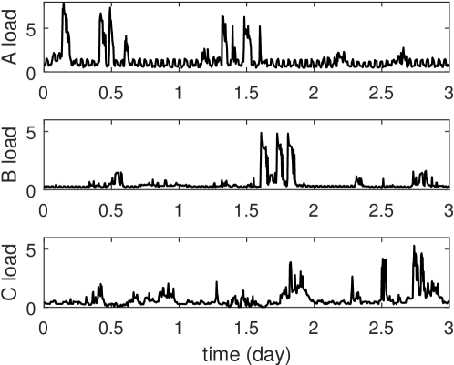
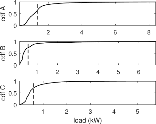
We analyze the Smart∗ Data Set obtained from the University of Massachusetts Trace Repository (Barker et al., 2012) to demonstrate customer consumption uncertainties. The specific data we use include the load data from three different homes located in Western Massachusetts given in one-second intervals from 33 days between May 1, 2012 through June 11, 2012, as well as the loads of another 395 buildings for one complete day. We average them into five-minute intervals and use these for our trace-based numerical studies. Five-minute intervals is the data granularity required by the ISO-NE (ISO new england, 2011) which is common among other DR programs (Federal Energy Regulatory Commission, 2010). A concurrent three day sample of the three homes is given in Figure 1(a), which shows peak loads are non-overlapping in many cases. Figure 1(b) displays the empirical cumulative distribution function of the three homes over the 33 days along with their means. The large peak-to-mean ratios indicate the significant uncertainties in customers energy consumptions.
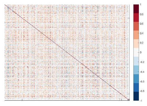
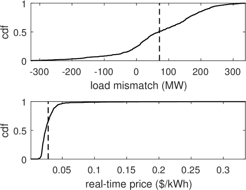
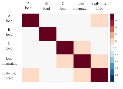
Furthermore, it is observed that customers’ loads are only weakly correlated, if at all. The northwest corner of Figure 2(c) shows a heatmap of the correlation matrix between the three homes which exhibits very little correlation. Similarly, for the loads of the other 395 buildings, a heatmap of the correlation matrix between 395 buildings is shown in Figure 1(c) which gives evidence that most customers have loads which are only weakly correlated.
2.2. Load Serving Entity Uncertainties
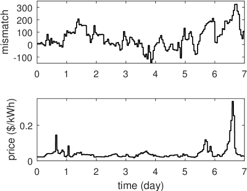
We analyze the following data from the ISO New England for the Western Massachusetts load zone (iso, 2016b) to demonstrate the market uncertainties LSE experience in their daily operation. The specific data is given in one-hour intervals of the real-time total load, load contracted in the day-ahead market, and the real-time market price for the same days as the previously described customer data. We calculate the real-time load mismatch of supply and demand as the difference between the real-time load and day-ahead market provisioned load. Figure 2(a) displays a one week sample of the load mismatch and its corresponding real-time price. The empirical cumulative distribution functions of the load mismatch and the real-time price for the 33 days are shown in Figure 2(b). The high peak-to-mean ratios indicate significant uncertainties in the load mismatch and prices that LSEs need to handle in real time. In addition, the southeast corner of Figure 2(c) shows that they are weakly correlated over the sampled 33 days.
2.3. A Dichotomy of Existing DR Programs
Existing DR programs in the current practice can be categorized by the commitment levels of the program participants. Most DR programs either demand the participants to fully commit to responding to DR signals, or allow the participants to not respond without any penalty at all. In what we refer to as fully committed DR programs, customers must respond to DR signals, and have to pay penalties if they fail to do so. Examples include CAISO BIP (Base Interruptible Program) (cai, 2016a), ERCOT ERS (Emergency Response Service) (erc, 2016), and NYISO SCR (Special Case Resources) (nyi, 2016). On the other hand we refer to voluntary DR programs as ones whose customers only voluntarily respond to DR signals in which ignoring DR signals is penalty-free. Examples include ERCOT VLR (Voluntary Load Response) (erc, 2016), NYISO EDRP (Emergency Demand Response Program) (nyi, 2016), and CAISO DBP (Demand Bidding Program) (cai, 2016b).
In between these two extremes with regard to customer commitment are voltage regulation services programs (e.g. PJM voltage regulation services (pjm, 2013; Chen et al., 2014)) which have relatively high payments for their fast control speed to follow a signal from the LSE (Aikema et al., 2012; Chen et al., 2015). The most interesting part of regulation services programs is the flexibility in them which motivates our LIN program described in Section 6.3. Instead of requiring customers to strictly follow the signal, there is a predefined violation frequency limit , i.e., customers can violate the signal up to of the time. Therefore, customers do not need to pay the high penalty even if they have some violations from the signal, as long as the probability of violation is below the predefined level. Intuitively, this can economically help the customers who may accidentally face high costs of DR and decide not to follow the signals.
2.4. Challenges of Customer Uncertainties
We end this section by highlighting the advantages and drawbacks of different commitment levels of DR programs. For a fully committed DR program, a) it has the advantage of providing guarantees to the LSE in getting the expected DR responses, but b) as such, it does not provide any flexibility to the participating customers in all but responding to DR signals, even though they may unexpectedly face a difficulty in real time in responding. For a voluntary DR program, a) it has the advantage that the customers are protected from their risks of having difficulty to respond to DR signals, but b) the LSE has a hard time of getting any reliability guarantees of the DR they get from such programs.
As a result, fully committed DR programs tend to enlist an insufficient amount of guaranteed DRs because customers are less willing to sign up due to their inherent uncertainties. On the other hand, voluntary DR programs face a similar consequence but for a different reason: it’s hard for them to obtain guaranteed DRs because customers can freely ignore any DR signals.
Recently, third-party curtailment service providers (CSPs) and aggregators pooling together DR from several customers emerge as a promising opportunity (Šikšnys and Pedersen, 2016). Our work can be viewed as a solution for CSPs and aggregators to lessen DR commitment uncertainties. For instance, the optimization problem and proposed algorithms can be adopted by CSPs and aggregators to allocate DR to their customers in a more effective way.
3. Model
We consider a discrete-time model with time step duration normalized to 1, such that price and demand changes can be updated within a time slot. There is a (possibly long) interval of interest , where can be one month, one year or even longer. Each timeslot represents the time needed to make changes to demand, which can be 5 minutes. This timescale is consistent with similar DR approaches as in (Harsha et al., 2013; Bitar et al., 2012).
There is an LSE who wishes to procure a total amount of load change. This can be load reduction as usual, and has the additional generalizability to handle the case for load increase when too much renewable energy is generated and/or customers demand is lower than predicted. The LSE serves a set of customers indexed by . We ignore the power network constraints in this paper. However, our model and algorithms can be extended with extra effort to incorporate those power network constraints. In particular, in a power distribution network, the exact convex relaxation and convexification (Low, 2014) can be applied to make the problem convex. Therefore the approach proposed in this paper can be applied.
Customers
Let be the total power demand of the appliances controlled by customer at time . To model the power demand uncertainty for customers we let be a random variable with lower and upper bounds and respectively. The LSE will predict customers’ demand to purchase power beforehand, e.g., in the day-ahead market. We denote by the predicted power consumption of customer at time .
In the real time, customer observes its own real power demand in the absence of a DR program and decides by under a particular DR program as the amount of demand change from . Here we use a positive as reduction, and a negative value implies demand increase. So the actual power consumption is . Essentially, we are using the actual consumption as the baseline to measure DR. Different baseline models can easily be incorporated with additional complexity. Determining customer baselines for demand response is an active area of research (Wijaya et al., 2014).
To model the loss of utility caused by the change in power consumption from the original demand , we assume there is a cost function . The function is inherently different for different timeslots. For instance, the customer may have some emergency tasks to finish at some timeslot, so changing the load is costly for that particular . It is not necessary for the change in demand to be instantaneous and the ramping time would be determined by the specific DR program. There are newly developed DR recommender systems (e.g. DR-Advisor (Behl et al., 2016)) that can be used by homeowners to manage DR commitments.
As usual, we make the following mild assumption about the customer’s cost/disutility function:
Assumption 1.
, is convex and differentiable with and .
Under this assumption, if the customers are left to decide their power consumption themselves without any demand response program, each customer will choose to consume at their power demand , i.e., . The convexity assumption is consistent with the concavity assumption of customer utility functions as was done in (Li et al., 2011; Jiang and Low, 2011; Bitar et al., 2012; Zhao and Low, 2014).
In reality, this cost function may not be known until at (or just before) the time of consumption. In some cases, the LSE needs to estimate the customers cost functions to set the appropriate price for demand response payment. Here, we assume that Assumption 1 also applies to the estimated customer cost function .
A simple but widely used example is the quadratic function, i.e., which is explored further in Section 4.2. The uncertainty of the function is therefore represented by the randomness in its parameter . While simple, quadratic cost functions are widely used in electricity market literature (Allaz and Vila, 1993; Yao et al., 2007; Murphy and Smeers, 2010; Cai and Wierman, 2013; Liu et al., 2014).
Load Serving Entity
We consider the general case where the LSE has volatile renewable energy generation that must be used when it is produced. The generation at time is denoted by a random variable bounded between and .
The LSE procures power beforehand according to its estimation on customers’ demand and renewable generations for timeslot . We assume the procurement is , while our model and approaches can be easily extended to handle other form of procurement.
After the power procurement, LSE is responsible for balancing in real time the power demand, which is the aggregate customer power consumption and the power supply, which consists of both the power procured beforehand, e.g., plus the available renewable power .
Therefore, the demand response goal is to clear the mismatch due to prediction errors, i.e.,
We denote by and the prediction errors for customer ’s demand and the renewable generation, respectively.
Then
In many cases, the LSE cannot get exactly amount of demand response, and has to bear the cost denoted by the penalty function , where . Specifically, this is the cost imposed on the LSE to close the gap through actions such as employing fast responding reserves or grid energy storage. We note that the cost of reducing some of the mismatch via hour-ahead (or other near-real-time) power market interactions can be incorporated in . Again, we make the following mild assumption:
Assumption 2.
is convex and differentiable with and .
In order for the LSE to tolerate the mismatch and prevent blackouts, the LSE must purchase long-term energy storage or reserves in some forward market denoted by . This gives us the mismatch constraint111This constraint can be generalized to the case where the upper and lower bounds are function of , and our approaches apply with little change.:
| (1) |
Notice that LSE’s decision for the capacity is constant for all where the time horizon is can be set to the time for deciding the capacity, e.g. a day, month, etc. Denote as the cost of the energy storage/reserve capacity amortized to the duration of interests . Again, we make the following mild assumption:
Assumption 3.
is increasing, convex and differentiable.
For instance, can be a quadratic function , and can be linear . While simple, quadratic cost functions are widely used in generation cost modeling (Park et al., 1993; Gaing, 2003; Hug, 2012).
Optimization Problem
The expected social cost can be represented by
where we assume that the randomness in customers’ cost function and the mismatch are stationary. This assumption is reasonable since the randomness in is due to the prediction error of the customers’ load demands and renewable energy supply. Additionally, this assumption is intuitive for customers whose underlying load preference behavior does not change significantly within the time horizon . Therefore, we can remove the time dependencies and simplify the expected social cost to:
| (2) |
where is amortized to a single timeslot.
The goal is therefore to decide the capacity planning and a practical policy simultaneously to optimize the expected social cost (2).
| (3a) | s.t. | |||
| (3b) | ||||
We note that (3a) and (3b) are worst-case constraints. To optimize the policy is known to be challenging, so we first provide the upper and lower bound to this optimization.
Upper bound: SEQ
The upper bound is the two-stage policy used widely in practice which first obtains capacity assuming the worst-case mismatch due to prediction error and then sets a price on voluntary DR. We call it “SEQ” in this paper to highlight it optimizes sequentially instead of simultaneously. In the first stage, SEQ performs capacity planning to obtain by solving the following optimization problem:
| (4) | ||||
| s.t. | ||||
Then in real-time, SEQ sets price to extract demand response from customers. This is to mimic the voluntary demand response programs such as NYISO EDRP.
Formally, SEQ works as:
SEQ: • Solve (4) to get for capacity planning; • In real time, pick a function to decide the demand response payment price when observing a mismatch .
Note how to pick the function highly depends on the experience and expertise of the LSE staffs. In Section 5, we propose a data-driven approach to obtain .
Lower bound: OFFLINE
A lower bound on the minimum social cost is given by the offline/a-posteriori optimal solution. Specifically, the offline optimum is given by the following:
| (5a) | s.t. | |||
Note that, the minimization over is performed inside the expectation, meaning that it is performed after observing the realizations of the random variables. This results in the fact that the offline optimum can never be beaten by any online policy .
Formally, OPT works as:
4. Characterizing the optima
In this section, we provide the characterization of the optimal solution to reveal special structures that we take advantage of in our algorithm design (Section 5). We start with the convexity of the problem followed by a concrete case study of the necessary and sufficient conditions of the optimal solution.
4.1. Convexity
The first key result regarding the problem is the convexity, as stated formally in Theorem 4.1. The convexity is crucial for our proposed algorithm in Section 5.
Theorem 4.1.
(5) is a convex optimization problem over .
The proof requires the following lemmas and we restate the real-time decision (i.e. inside the expectation) of Problem (5) as:
| (6a) | ||||
| (6b) | s.t. | |||
Lemma 4.2.
Problem (6) is a convex optimization problem.
Proof.
Lemma 4.3.
4.2. Case study: quadratic cost functions
To provide more optimal structures, we restrict ourselves to the quadratic cost functions, i.e. and . Their key advantageous property is that have linear marginal costs which allow for more concrete analysis and motivate the linear decision policy (Section 5.2). Note this may seem restrictive, but this form is standard within the electricity markets literature, e.g., (Allaz and Vila, 1993; Yao et al., 2007; Murphy and Smeers, 2010; Cai and Wierman, 2013; Liu et al., 2014) and generation cost modeling (Park et al., 1993; Gaing, 2003; Hug, 2012).
Then the offline optimization problem in real-time without capacity constraints222This can be added with additional presentation complexity. becomes:
By the first-order stationary conditions from the Karush-Kuhn-Tucker (KKT) conditions (See Appendix A for the general case), we have
Sum over all gives:
Finally, we have , which is linear to the social mismatch . This property is crucial to help us design the linear policy. This approach is general and can be applied to more complicated cost functions. The difference is that the optimal structure would be more complicated, and so would the policy.
5. Algorithms
In this section, we design two algorithms/control policies for DR, namely, “PRED” and “LIN”. PRED is the prediction based policy with no contracts, and is hence a voluntary program. LIN relies on a linear demand response contract between LSE and customers, and is hence a mandatory program: it, however, respects customer uncertainties as will be shown later in this section. For presentation simplicity, we omit the and will highlight it wherever needed.
5.1. Prediction Based Policy
Ideally, the LSE would like to set a price for demand response and obtain an amount that would optimally solve Problem (6). This in turn would allow Problem (5) of finding the optimal capacity to be solved.
In general however, the customer cost functions and the instantaneous customer load deviations are not known by the LSE. Despite this, from historical data of past customer responses to prices, the LSE can estimate their cost functions denoted by with some inaccuracies.
From a privacy perspective, customers may not be willing to share their detailed load data due to the information that can be inferred from it. However, customers can hide some of their private information by recently proposed mechanism, e.g., using batteries to add randomness to their consumptions (Zhao et al., 2014; Laforet et al., 2016).
First, the LSE utilizes the historical data to solve a (deterministic) optimization problem about how to set the price for demand response, i.e., for a given . For a given it optimizes:
| (7) | ||||
| s.t. |
We abuse the notation of as to represent a customer’s demand response given a particular price .
To find the optimal amount of capacity , it must solve
| (8) |
which may be done by exhaustive search for the best . Once is fixed, then the optimal solution to (7) gives a price function . This price function is then applied in real-time to obtain demand response from all the customers. Under certain conditions, such as quadratic and/or linear cost functions, a closed form of can be obtained.
Formally, PRED works as follows:
PRED: • Using historical date to solve (7) to get ; • Solve (8) to get for capacity planning; • In real time, when observing , set price .
PRED is intuitive and works well when the uncertainties on are small, as illustrated in the numerical evaluations in Section 6. This makes PRED an attractive solution in many cases. For instance, in the emergency demand response program, the LSE sets the price based on their knowledge and experience, which corresponds to the predicted in our PRED scheme. We would like to highlight that by proposing PRED, we are making two improvements over existing schemes. First, we provide a rigorous procedure to get by looking into historical data and solving an optimization problem. Second, we jointly solve and , instead of getting them sequentially in SEQ.
However, its performance greatly depends on the estimation accuracy of the cost functions, and degrades as the uncertainties increase. To see this, note that the LSE needs to pick based on some sort of “averaged” customers’ cost functions, without knowing the exact realization of . When has more uncertainties, the response from customers based on the realized may be farther away from the value expected by the LSE.
5.2. Linear policy
Motivated by the potential inefficiency of PRED when uncertainties are large, we design a linear policy, “LIN”, as the contract between LSE and customers.
In general, we can take the following nonlinear form of a customer demand response policy:
| (9) |
where is a function of net aggregate mismatch , and is function of the local demand mismatch. This structure is rich enough for the demand change to be responsive to the net society mismatch through , local self mismatch through , and an independent reduction of .
While the above form is general and powerful, there are two concerns around it. First of all, in addition to the parameter , we need to optimize over the function form and , which is very challenging, if not impossible. More importantly, customers may not be willing to accept contracts in a very complicated form. Based on these considerations, we restrict our attentions to the following linear policy, and show that this policy works very well in many cases, in particular, when cost functions are quadratic. How to decide the optimal and for general convex cost functions is our future work.
We now focus on a simple but powerful linear demand response policy that is a function of total and local net demands:
| (10) |
Intuitively, there are three components: implies each customer shares some (predefined) fraction of the global mismatch ; means customer may need to take additional responsibility for the mismatch due to his own demand fluctuation and estimation error; finally, , the constant part, can help when the random variables and/or is nonzero. In fact, this linear policy is optimal for the case of quadratic cost functions which can be seen in Section 4.2.
Then the LSE needs to solve the following optimization problem to obtain the optimal parameters for the linear contract, i.e., , as well as the optimal capacity :
| (11) | ||||
| s.t. |
The expectation can be separated by customer and LSE because of the linearity of expectation property.
Theorem 5.1.
Problem (11) is a convex optimization problem.
Proof.
The objective function is convex in because the expectation operator preserves convexity, the cost functions are convex from Assumptions 1-3, and the arguments inside each cost function are linear in for each realization of which preserve convexity. By substituting the linear policy (10) into constraints (3a), (3b) it forms a convex set because the point-wise maximum (minimum) operator preserves convexity (concavity), and the arguments inside the operators are linear in for each realization of which preserve convexity (concavity). The result follows from the objective function being convex and the constraint set forming a convex set. ∎
Since Problem (11) is a convex optimization problem and is also stochastic, it can be solved centrally with standard stochastic optimization techniques such as the Stochastic Subgradient Method with Monte Carlo sampling where one simulates a sample of and solves the problem via the dual variables by taking a step in the direction of the dual variables’ subgradient . As the number of iterations approaches infinity, then the dual variables approach their optimal values (Boyd and Mutapic, 2014). If the cost functions are quadratic and/or linear then only the first and second moments of and are needed to make (11) into a deterministic convex optimization problem.
Formally, LIN works as:
LIN: • Solve (11) to get for capacity planning and the parameters ; • In real time, customer needs to provide demand response when observing .
5.3. Distributed algorithm design
In many cases, the LSE may not know the information about customers’ cost functions, and cannot solve (11) for the parameters in the linear contract. To handle this, we design the distributed algorithm to decompose the problem, so that each customer solves an optimization problem based on her own cost function, and LSE solves another optimization problem without knowing the customers’ cost function. The goal is to achieve the optimal .
To decompose Problem (11) we use the auxiliary variables for in the estimated cost function of each customer, and add the constraints that , , and :
| (12a) | s.t. | |||
| (12b) | ||||
Problem (12) can be split where each customer controls its own and the LSE controls from the dual decomposition of constraint (12b). Let be the dual prices for each customer corresponding to constraint (12b) which result in the following meanings: is the price paid for the guaranteed reduction in power consumption by the customer, is the price paid for absorbing the fraction of the net aggregate system demand , is the price paid for absorbing the fraction of its own local net demand . Therefore is the total payment to customer for following the linear demand response policy.
Accordingly, (11) is decomposed as the individual customer optimization problem,
| (13) |
and the LSE’s optimization problem,
| (14) | ||||
| s.t. |
which both can be solved with standard stochastic optimization techniques such as the Stochastic Subgradient Method with Monte Carlo sampling (Boyd and Mutapic, 2014). With linear or quadratic cost functions, they in fact can be solved as a deterministic convex optimization problem with only the first and second order moments of and . The goal now becomes to find the optimal dual prices to ensure the customers’ and LSE’s decisions satisfy (12b). We achieve this by using the Subgradient Method (see (Bertsekas, 1999) Chapter 6):
Distributed Algorithm for LIN: (0) Initialization: . (1) LSE: receives from each customer . • Solves Problem (14) and updates with the optimal solution. • Updates the stepsize: (15) where is a small constant and is the iteration number. • Updates the dual prices, : (16) • Sends to the each customer respectively. (2) Customer : receives from LSE. • Solves Problem (13) and updates with optimal solution. • Sends to the LSE. (3) Repeat Steps 1-2 until where is the tolerance on magnitude of the subgradient.
Since the step size is non-summable, square summable, and diminishes to zero, the algorithm will converge to an equilibrium point. Then the final agreed values are last sent by the customers, and the dual prices are last sent by the LSE. When the LSE signals the customers for DR and they respond accordingly, they will each be paid .
We now prove the convergence and optimality using two mild technical conditions:
Assumption 4.
The distance between the first iteration of the distributed algorithm and the optimal dual prices has a finite upper bound: .
Assumption 5.
The magnitude of the dual subgradient has a finite upper bound: (i.e. the Lagrangian dual function is Lipschitz continuous).
Theorem 5.2.
The proof has been relegated to Appendix B.
6. Performance Evaluation

We compare our proposed algorithms PRED and LIN with two baselines: the offline optimal solution OPT as the lower bound for social cost and the sequential algorithm SEQ as the upper bound.
6.1. Experimental Setup
We aim to use realistic parameters in the experimental setup to evaluate the performance of our proposed algorithms, and to understand the solution properties of each algorithm. We model an LSE supplying power to 300 customers with a demand response timeslot that is five minutes long.
The LSE first purchases capacity for which we model the cost as a linear function with the parameter /kW-mo to cover a broad range of grid capacity type costs and amortized storage. The generation cost function for the LSE is modeled as a quadratic function with the parameter . For this cost function setting, a deviation of 60kW for five minutes is equivalent to an energy cost of $0.50/kWh and matches the intuition that larger mismatches are increasingly more expensive to manage.
To model each customer’s particular load demand, we utilize the traces obtained from the UMass Trace Repository which give very granular load measurements from three homes (cf. Figure 1(b) for cumulative distributions) (Barker et al., 2012). To make more accurate general conclusions we need more customers’ load data. However, the focus of this evaluation is to compare the performance of the different algorithms presented and demonstrate how to employ customer data to them. We model the cost incurred by each customer to change its consumption as a quadratic cost with the parameter . Under these settings, a consumption decrease of 0.3kW for five minutes would cost the customer an energy price equivalent to $0.025-0.25/kWh. To generate customer cost uncertainties we first randomly choose from a bounded normal distribution. Each is used as a mean to further generate the training and test sets separately from a bounded normal distribution. The approximated by the LSE is then formed by averaging the training set values for customer .
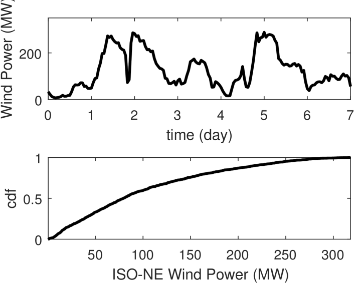
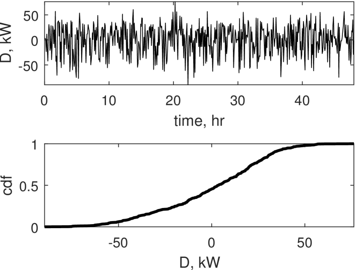
Renewable generation is incorporated into our simulations by using the ISO-NE’s data on hourly wind power production for the same dates as the UMass data (iso, 2016a). A week-long sample and cumulative distribution for all the data are shown in Figure 3. The capacity is set to 100kW by default, while we vary it in the sensitivity analysis. The training and test sets for which we have trace data (Homes A,B,C and ISO-NE wind production) were made by first randomly separate each trace into a raw training and raw test set. For each set we generate customer traces by bootstrapping 100 customers from each of the UMass Homes A/B/C. We also do this for the ISO-NE wind data which is first normalized by the maximum power output so that we can scale wind power. The demand mismatch over two days and the corresponding CDF are depicted in Figure 4.
6.2. Performance evaluation
The evaluation of our algorithms and the cost savings will be organized around the following topics.
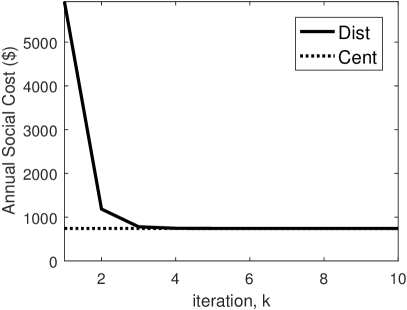
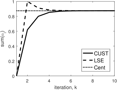
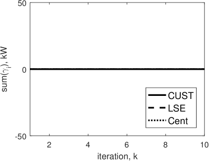
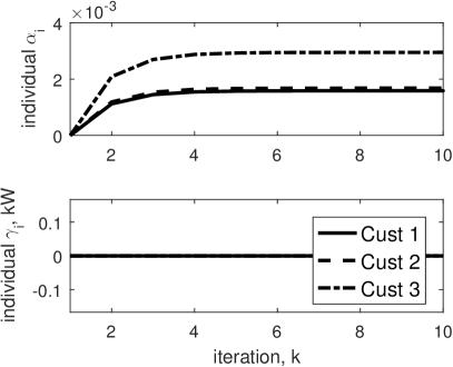
Convergence of the distributed algorithm
We start by considering the convergence of our distributed algorithm for LIN. Figure 5(a) illustrates that the social cost of the distributed algorithm converges quickly to that of the centralized algorithm which validates the convergence analysis of Theorem 5.2. For the parameters, even if we start with , it quickly converges to the optimal which are different among customers as they have different parameters, i.e., in their cost functions. For the other LIN parameters, and stay at zero across all customers since the optimal for zero-mean deviations and optimal for quadratic cost functions. Thus, the remaining plots show only the centralized algorithm.
How well do PRED and LIN perform?
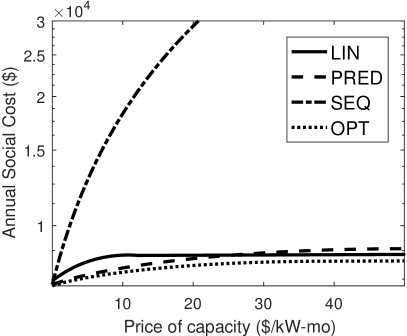
We move to this key question of the evaluation. To evaluate the benefits in terms of social cost savings for our algorithms, Figure 6 compares the social cost of PRED and LIN to those under the offline optimal OPT and sequential algorithm SEQ. Since OPT requires knowledge about each realization of the parameters, i.e., the exact renewable generation, customers’ demand and cost functions at each timeslot, it is not practically feasible. We simply use this as a lower bound of the social cost. However, SEQ makes conservative capacity planning decision about first, and then performs similar to PRED. By comparing to the cost of SEQ, the benefit of joint optimization of capacity planning on and real-time demand response is highlighted.
The social costs of PRED and LIN, shown in Figure 6(a), are no more than higher compared to the fundamental limit OPT. Importantly, when the capacity price decreases, the gap between PRED/LIN and OPT becomes smaller. Since currently the technology improvements are reducing the capacity price, from Figure 6(a), this gap will decrease further. The social cost of SEQ increases rapidly with increasing capacity prices because of the conservative 90kW capacity used to protect the system from any leftover mismatch.
When capacity price increases, all algorithms have higher costs as expected. However, PRED increases faster than LIN. This is because LIN starts to rely more on the linear contracts than capacity, so it becomes more immune to the capacity price increases. This provides the first guideline to choose between PRED and LIN in practice. The second guideline depends on the level of customers’ uncertainties, and will be discussed soon.
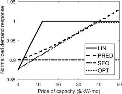
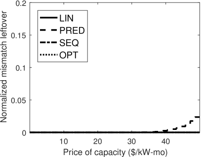
Interestingly, for PRED, LIN, and OPT, the social cost flatten when the price exceeds some threshold. This is because when capacity price is too high, the LSE would purchase little capacity, as shown in Figure 6(b) and pay more to get demand response from customers, illustrated by Figure 6(c). The downside in the case of PRED, however, is the increased remaining mismatch that is not balanced by demand response, as shown in Figure 6(d).
To understand more behind the social costs, Figures 6(b) and 6(c) illustrate the optimal capacities and the amount of demand response extracted for all algorithms. As the price increases, the capacities decrease, and the amounts of extracted DR increase to compensate for the reduced reserve capabilities. Note in Figure 6(b), PRED always has a higher capacity than OPT because PRED needs some additional capability to handle the estimation errors. Similarly, when setting the price, PRED picks a higher price to extract more demand response on average, as shown in Figure 6(c), to act as a buffer in case some customers’ responses are overestimated. The increased cost due to uncertainties in PRED compared to OPT can be considered as a “risk premium”. We will vary the customers’ uncertainties to provide more information in Figure 8.
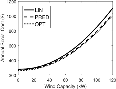
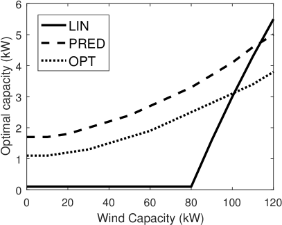
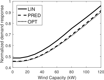
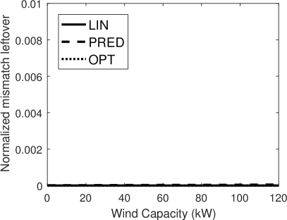
Impacts of the renewable penetration level.
As renewable energy installation is rapidly growing, we evaluate the impacts of installed renewable energy capacities. Illustrated by Figure 7, social cost increases with more renewable energy installed as there is larger mismatch to be balanced. When the wind capacity is too large, LIN can no longer just rely on the demand response, but needs a higher capacity, as shown in Figure 7(b). Throughout the figures, our proposed algorithms PRED and LIN perform very closely to the offline OPT.
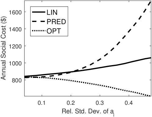
Impacts of customer uncertainties.
As another key message of the paper, we investigate the impact of the customer cost function uncertainties through the parameter . Here we fix the average cost parameter and vary the variance of .
Figure 8 illustrates the social cost of the algorithms under different relative standard deviations. Interestingly, as the variance increases, OPT actually has a lower cost. The reason is that since OPT is the offline solution, it can utilize the realization of each to target the customers with small cost parameters for each timeslot . As the variance increases, this targeted set of customers will have lower parameters, which leads to lower social cost in OPT.
PRED has the same cost as OPT when the variance is 0, but the gap becomes larger as the variance increases. Unlike the case of increasing uncertainty from larger renewable capacities, the increased uncertainties due to a larger variance in cannot be well handled by PRED. However, the cost of LIN does not change much. This suggests the second rule to pick between PRED and LIN: with larger uncertainties, LIN performs relatively better.
6.3. Flexible Commitment Demand Response
6.3.1. LIN with flexibility: LIN
One potential drawback of LIN is that customers are forced to follow the specified linear policy and may from time-to-time face a very high cost to follow the policy. From the social perspective, it is not beneficial to force a customer under much higher than average costs to provide demand response as compared to the LSE cost for tolerating more mismatch.
Motivated by this observation and the regulation service program described in Section 2, we modify the LIN policy to add some flexibility limited by a single parameter . We call the new algorithm LIN. Under LIN, each customer has up to (in percentage) of the timeslots in which they do not need to follow the policy according to her realized . In other words, she may pick her original with for such timeslots.
A caveat is that we add is to only allow the customers to pick such timeslots according to their cost functions, e.g., through the parameters regardless of . From the social perspective, allowing customers with higher to violate results in lower social costs. However if the customers had full freedom, most customers would choose to violate when is high which is when the LSE needs DR the most. In reality, this condition can be enforced by calculating for the timeslots that a particular customer chooses to violate. If this value is significantly higher than , then the customer faces some penalty.
Note that although we add the flexibility to LIN in this paper, the approach is in fact general and can be applied to a wide range of fully committed programs as follows. Each customer is allowed to violate her commitment by up to (in percentage) of the timeslots. A customer can run a local optimization to decide which timeslots to violate, while the LSE can add some constraints to align the local optimization with the social optimization, such as those described above.
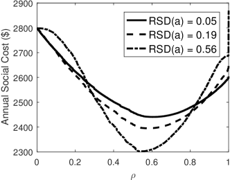
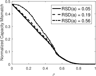
6.3.2. Cost versus mismatch leftover tradeoff
Now we evaluate the additional cost savings brought by LIN. Figure 9 highlights the tradeoff between cost and mismatch leftover that cannot be balanced due to capacity constraints. Recall that there is little mismatch leftover in LIN, or equivalently, LIN+(1).
Depicted in Figure 9(a), as decreases from 1, the social cost first decreases due to the fact that some customers with very high are allowed to not provide demand response. As continues to decrease, we have more customers not providing demand response and the cost actually goes up again. This is because the penalty for the mismatch becomes larger than the costs of customers to provide demand response.
On the other hand, Figure 9(b) highlights that the mismatch leftover increases with lower as more customers are allowed to not provide demand response. Importantly, the increase is very slow at the beginning when we decrease from because there is enough capacity to handle the small deficit in demand response. However, the social cost decreases a lot. This actually highlights the great potential to decrease appropriately to achieve a lower social cost but still have little mismatch leftover. For instance, in our case study shown in Figure 9, achieves cost savings 7-8% with less than 1% of mismatch leftover. Recall that the gap between LIN and the offline optimal OPT is about 10%. This means LIN achieves near optimal cost.
7. Conclusion
Extracting reliable demand response from customers is crucial to reduce/defer new energy storage/reserve installation and has significant environmental benefits. However, existing demand response programs suffer from either low participation due to strict commitment, or not being reliable in voluntary programs. Moreover, the capacity planning for energy storage/reserve is traditionally done without considering the demand response capabilities, which incurs inefficiencies. Additionally, the uncertainties on the customers costs in providing demand response receive little attention in literature. In this paper, we first model the problem as a stochastic optimization problem, and then design two online algorithms, PRED and LIN, to jointly optimize the capacity and demand response program design. PRED utilizes historical data to estimate the cost functions, while LIN is a linear contract between the LSE and customers. We further design a distributed algorithm with guaranteed convergence for obtaining the optimal parameters for LIN. In addition, we design a flexible commitment demand response program LIN by adding flexibility to LIN. Numerical simulations highlight the near optimal performance of the proposed algorithms, and large cost savings compared to a widely used baseline SEQ especially when capacity price is not negligible.
Regarding further directions, the most exciting one is to incorporate power network constraints into our optimization framework. This will bring some new challenges and insights. In particular, the parameter for the customer’s own prediction error in LIN will no longer be zero due to the fact that errors can be handled easier locally because of the loss over power lines and the line capacity constraints.
8. Acknowledgments
We thank all of the reviewers and our shepherd Shaolei Ren for their valuable feedback. This research is supported by NSF grants CNS-1464388 and CNS-1617698.
References
- (1)
- pjm (2013) 2013. PJM, Market-Based Regulation [Online]. http://pjm.com/markets-and-operations/ancillary-services. (2013).
- cai (2016a) 2016a. CAISO, Base Interruptible Program [Online]. https://www.pge.com/en_US/business/save-energy-money/energy-management-programs/demand-response-programs/base-interruptible/base-interruptible.page. (October 2016).
- cai (2016b) 2016b. CAISO, Demand Bidding Program [Online]. https://www.pge.com/en_US/business/save-energy-money/energy-management-programs/demand-response-programs/demand-bidding/demand-bidding.page. (October 2016).
- sgd (2016) 2016. Department of Energy, The smart grid: an introduction [Online]. http://energy.gov/oe/downloads/smart-grid-introduction-0. (March 2016).
- erc (2016) 2016. ERCOT, Demand Response [Online]. http://www.ercot.com/services/programs/load. (October 2016).
- CPP (2016) 2016. Fort Collins Utilities, Coincident peak [Online]. http://www.fcgov.com/utilities/business/rates/electric/coincident-peak. (October 2016).
- iso (2016a) 2016a. ISO New England, Daily Generation by Fuel Type [Online]. https://www.iso-ne.com/isoexpress/web/reports/operations/-/tree/daily-gen-fuel-type. (September 2016).
- iso (2016b) 2016b. ISO New England, Zonal Information [Online]. http://www.iso-ne.com/isoexpress/web/reports/pricing/-/tree/zone-info. (May 2016).
- nre (2016) 2016. National Renewable Energy Laboratory, Variability of Renewable Energy Sources [Online]. http://www.nrel.gov/electricity/transmission/variability.html. (April 2016).
- nyi (2016) 2016. NYISO, Demand Response Programs [Online]. http://www.nyiso.com/public/markets_operations/market_data/demand_response/index.jsp. (October 2016).
- doe (2016) 2016. US Department of Energry, Grid Integration [Online]. http://energy.gov/eere/wind/grid-integration. (April 2016).
- Aikema et al. (2012) D. Aikema, R. Simmonds, and H. Zareipour. 2012. Data centres in the ancillary services market. In IGCC. 1–10.
- Allaz and Vila (1993) Blaise Allaz and Jean-Luc Vila. 1993. Cournot competition, forward markets and efficiency. Journal of Economic theory 59, 1 (1993), 1–16.
- Barker et al. (2012) Sean Barker, Aditya Mishra, David Irwin, Emmanuel Cecchet, Prashant Shenoy, and Jeannie Albrecht. 2012. Smart*: An open data set and tools for enabling research in sustainable homes. SustKDD, August 111 (2012), 112.
- Behl et al. (2016) Madhur Behl, Francesco Smarra, and Rahul Mangharam. 2016. DR-Advisor: A data-driven demand response recommender system. Applied Energy 170 (2016), 30–46.
- Bertsekas (1999) Dimitri P Bertsekas. 1999. Nonlinear programming. Athena scientific Belmont.
- Bitar et al. (2012) Eilyan Bitar, Kameshwar Poolla, Pramod Khargonekar, Ram Rajagopal, Pravin Varaiya, and Felix Wu. 2012. Selling Random Wind. In System Sciences, Hawaii International Conference on. IEEE, 1931–1937.
- Bitar et al. (2011) Eilyan Bitar, Ram Rajagopal, Pramod Khargonekar, and Kameshwar Poolla. 2011. The role of co-located storage for wind power producers in conventional electricity markets. In American Control Conference (ACC). IEEE, 3886–3891.
- Boyd and Mutapic (2014) Stephen Boyd and Mutapic. 2014. Lecture notes on Stochastic Subgradient Methods. (April 2014).
- Boyd and Park (2014) Stephen Boyd and Jaehyun Park. 2014. Lecture notes on Subgradient Methods. (May 2014).
- Boyd and Vandenberghe (2004) S. Boyd and L. Vandenberghe. 2004. Convex Optimization. Combridge University Press.
- Cai and Wierman (2013) Desmond WH Cai and Adam Wierman. 2013. Inefficiency in forward markets with supply friction. In 52nd IEEE Conference on Decision and Control. IEEE, 5594–5599.
- Chen et al. (2014) H. Chen, M. C. Caramanis, and A. K. Coskun. 2014. The data center as a grid load stabilizer. In Design Automation Conference (ASP-DAC), IEEE 19th Asia and South Pacific. 105–112.
- Chen et al. (2015) Hao Chen, Zhenhua Liu, Ayse K Coskun, and Adam Wierman. 2015. Optimizing energy storage participation in emerging power markets. In Green Computing Conference and Sustainable Computing Conference (IGSC), 2015 Sixth International. IEEE, 1–6.
- Cherry (2013) Brian K. Cherry. 2013. Electric Schedule E-CBP. Technical Report. Pacific Gas and Electric Company.
- Chowdhury et al. (2016) M. Chowdhury, M. Rao, Y. Zhao, T. Javidi, and A. Goldsmith. 2016. Benefits of storage control for wind power producers in power markets. to appear in IEEE Transactions on Sustainable Energy (2016).
- Federal Energy Regulatory Commission (2010) Federal Energy Regulatory Commission 2010. FERC-731 Demand Response/Time-Based Rate Programs and Advanced Metering instructions. Federal Energy Regulatory Commission.
- Framework (2010) NIST Framework. 2010. Roadmap for Smart Grid Interoperability Standards, Release 1.0 (Jan. 2010)(NIST Special Publication 1108). (January 2010).
- Gaing (2003) Zwe-Lee Gaing. 2003. Particle swarm optimization to solving the economic dispatch considering the generator constraints. IEEE transactions on power systems 18, 3 (2003), 1187–1195.
- Harsha et al. (2013) Pavithra Harsha, Mukesh Sharma, Ramesh Natarajan, and Sudip Ghosh. 2013. A framework for the analysis of probabilistic demand response schemes. Smart Grid, IEEE Transactions on 4, 4 (2013), 2274–2284.
- Hug (2012) Gabriela Hug. 2012. Generation cost and system risk trade-off with corrective power flow control. In Communication, Control, and Computing (Allerton), 2012 50th Annual Allerton Conference on. IEEE, 1324–1331.
- ISO new england (2011) ISO new england 2011. Demand Resource (DR) User Interface Guide (RL.2 ed.). ISO new england.
- Jiang and Low (2011) Libin Jiang and Steven Low. 2011. Multi-period optimal energy procurement and demand response in smart grid with uncertain supply. In Decision and Control and European Control Conference. IEEE, 4348–4353.
- Kirby (2005) Brendan J Kirby. 2005. Frequency regulation basics and trends. United States. Department of Energy.
- Laforet et al. (2016) Fabian Laforet, Erik Buchmann, and Klemens Böhm. 2016. Towards provable privacy guarantees using rechargeable energy-storage devices. In Proceedings of the Seventh International Conference on Future Energy Systems. ACM, 7.
- Li et al. (2011) Na Li, Lijun Chen, and Steven H Low. 2011. Optimal demand response based on utility maximization in power networks. In 2011 IEEE power and energy society general meeting. IEEE, 1–8.
- Liu et al. (2014) Zhenhua Liu, Iris Liu, Steven Low, and Adam Wierman. 2014. Pricing data center demand response. ACM SIGMETRICS Performance Evaluation Review 42, 1 (2014), 111–123.
- Low (2014) Steven H Low. 2014. Convex relaxation of optimal power flow, part I: Formulations and equivalence. arXiv preprint arXiv:1405.0766 (2014).
- Murphy and Smeers (2010) Frederic Murphy and Yves Smeers. 2010. On the impact of forward markets on investments in oligopolistic markets with reference to electricity. Operations research 58, 3 (2010), 515–528.
- New York Independent System Operator (2013) New York Independent System Operator 2013. Emergency Demand Response Program Manual (7.1 ed.). New York Independent System Operator, Rensselaer, NY.
- Park et al. (1993) JH Park, YS Kim, IK Eom, and KY Lee. 1993. Economic load dispatch for piecewise quadratic cost function using Hopfield neural network. IEEE Transactions on Power Systems 8, 3 (1993), 1030–1038.
- Peterman (2013) Carla J. Peterman. 2013. R. 10-12-007 COM/CAP/jv1. California Public Utilities Commission (October 2013).
- Pinson (2013) P. Pinson. 2013. Wind energy: Forecasting challenges for its operational management. Statist. Sci. 28, 4 (2013), 564–585.
- Šikšnys and Pedersen (2016) Laurynas Šikšnys and Torben Bach Pedersen. 2016. Dependency-based FlexOffers: scalable management of flexible loads with dependencies. In Proceedings of the Seventh International Conference on Future Energy Systems. ACM, 11.
- Silverstein (2013) Ken Silverstein. 2013. California’s New Energy Storage Mandate Under the Microscope. Online, EnergyBiz (October 2013). http://www.energybiz.com/article/13/10/california-s-new-energy-storage-mandate-under-microscope.
- Skinner (2010) Nancy Skinner. 2010. Assembly Bill No. 2514. California State Assembly (September 2010).
- Vardakas et al. (2015) John S. Vardakas, Nizar Zorba, and Christos V. Verikoukis. 2015. A Survey on Demand Response Programs in Smart Grids: Pricing Methods and Optimization Algorithms. IEEE Communcation Suverys Tutorials 17, 1 (2015), 152–178.
- Wierman et al. (2014) Adam Wierman, Zhenhua Liu, Iris Liu, and Hamed Mohsenian-Rad. 2014. Opportunities and challenges for data center demand response. In Green Computing Conference (IGCC), 2014 International. IEEE, 1–10.
- Wijaya et al. (2014) Tri Kurniawan Wijaya, Matteo Vasirani, and Karl Aberer. 2014. When bias matters: An economic assessment of demand response baselines for residential customers. IEEE Transactions on Smart Grid 5, 4 (2014), 1755–1763.
- Yao et al. (2007) Jian Yao, Shmuel S Oren, and Ilan Adler. 2007. Two-settlement electricity markets with price caps and Cournot generation firms. european journal of operational research 181, 3 (2007), 1279–1296.
- Zhao and Low (2014) Changhong Zhao and Steven Low. 2014. Optimal decentralized primary frequency control in power networks. In 53rd IEEE Conference on Decision and Control. IEEE, 2467–2473.
- Zhao et al. (2014) Jing Zhao, Taeho Jung, Yu Wang, and Xiangyang Li. 2014. Achieving differential privacy of data disclosure in the smart grid. In INFOCOM, 2014 Proceedings IEEE. IEEE, 504–512.
- Zhao et al. (2015) Yue Zhao, Junjie Qin, Ram Rajagopal, Andrea Goldsmith, and H Vincent Poor. 2015. Wind aggregation via risky power markets. Power Systems, IEEE Transactions on 30, 3 (2015), 1571–1581.
Appendix
Appendix A Karush-Kuhn-Tucker conditions
Karush-Kuhn-Tucker (KKT) conditions for optimality of at time in Problem (6) are:
| (17a) | |||
| (17b) | |||
| (17c) | |||
| (17d) | |||
| (17e) |
where are the dual variables for the constraint (6b), (17a) are the first-order stationary conditions, (17c) and (17b) are the complementary slackness conditions, (17d) are the dual feasibility conditions, and (17e) are the primal feasibility conditions.
To better understand the physical implications of these conditions, we start from (17b) and (17c). When the constraint (17e) on is non-binding, i.e., , we have . Then (17a) implies , meaning that the marginal cost for each customer to provide demand response is the same, all of which is equal to the LSE’s marginal cost to tolerate the mismatch.
The KKT condition of optimality for capacity in Problem (5) is:
| (18) |
where is the optimal value of Problem (6). We can interchange the derivative operator and expectation operator if either of the following conditions are true: (i) are from continuous probability distributions and is continuously differentiable for all (from the Leibniz Integral Rule); (ii) are from discrete probability distributions (differentiation is a linear operator). This results in the following:
| (19) |
From Lemma 4.3, the negative of the sum of the dual variables for constraint (6b) is the gradient of w.r.t. . This allows us to substitute for the partial derivative:
| (20) |
where we use the notation of as a function to represent the sum of the optimal dual variables from the KKT conditions (17) for given .
Appendix B Proofs
Proof of Theorem 5.
(Based on (Boyd and Park, 2014) and (Bertsekas, 1999) Chapter 6.) At iteration , let be the current dual prices, be the partial dual function value of (12), be the subgradient of the dual function, and be the step size. Also note that the subgradient at iteration k for constraint (12b) is .
Start with the squared Euclidean distance between the iteration and optimal dual price vectors and substitute with the dual price update in Equation (16):
| (21) |
Expanding out the terms on the RHS becomes:
| (22) |
The first-order condition of the subgradient is which when applied to the equation above gives us:
| (23) |
Apply the above inequality recursively from iteration to which results in:
| (24) |
Since , then the LHS of the above inequality is lower bounded by zero and the middle term of the RHS can be brought to the other side:
| (25) |
Let us define as the best dual value so far in iterations. This gives a new lower bound to the LHS of the above inequality and allows the summation to be factored out:
| (26) |
and can be brought to the RHS:
| (27) |
Apply the definition of the step size from (15) which turns the above inequality into:
| (28) |
The Assumptions 4 and 5 give an upper bound on the RHS on the above inequality and allows to be factored out:
| (29) |
Taking the limit as number of iterations approaches infinity makes the RHS approach zero. Also since the LHS is lower bounded by zero, this results in the best dual value converging to the optimal dual value. Since dual the function is continuous, then . ∎
In ensuring the existence of the optimal solution to (12), we state the following theorem.
Definition B.1.
Theorem B.2.
There exists a set of equilibrium prices , LSE DR settings , and customer DR settings . Additionally, the set is optimal to (12).
Proof.
If one takes the Lagrangian of (12), it can be noticed that it equals the sum of LSE’s Lagrangian of (14) and all the customers’ Lagrangians of (13). Also, the set of primal feasible solutions of (12) is a subset of primal feasible solutions of (14) and (13) for each customer . Additionally, the dual feasible set and complementary slackness constraints coming from (3a)(3b) applies to both (12) and (14). Therefore a solution that satisfies the Karush-Kuhn-Tucker (KKT) conditions of (12) also simultaneously satisfies the KKT conditions of (14) and (13), with the condition that . An equilibrium point from Definition B.1 must also satisfy KKT conditions of (14) and (13), with the condition that . Since (12),(14), and (13) are convex optimization problems, the KKT conditions are both necessary and sufficient for optimality. Since there clearly exists an optimal point of (12), then there must exist an equilibrium point. It can be checked that the KKT conditions of (14) and (13), along with are equivalent to the KKT conditions of (12). Therefore an equilibrium point is optimal to (12). ∎