Quadrature readout and generation of squeezed states of a harmonic oscillator using a qubit-based indirect measurement
M. Canturk
Institute for Quantum Computing, Department of Mechanical and Mechatronics Engineering, and Waterloo Institute for Nanotechnology, University of Waterloo, Waterloo, ON, Canada N2L 3G1
A. Lupascu 111Corresponding author: adrian.lupascu@uwaterloo.caInstitute for Quantum Computing, Department of Physics
and Astronomy, and Waterloo Institute for Nanotechnology, University
of Waterloo, Waterloo, ON, Canada N2L 3G1
adrian.lupascu@uwaterloo.ca
Abstract
We present a protocol for measuring the quadrature of a harmonic oscillator (HO). The HO is coupled to a qubit, with an interaction modulated by the qubit control and effectively proportional to the HO quadrature . Repeated measurement of the qubit leads to gradually increasing information on the quadrature , leading to squeezing. We derive an analytical formula for the quadrature variance, , with the product of interaction strength and interaction time and the number of repetitions of the measurement. We discuss the robustness of this scheme against decoherence. We find that this protocol could lead to significant squeezing in a realistic setup formed of a superconducting flux qubit used to measure an electrical or mechanical resonator.
Introduction.— The quadratures of a quantum harmonic oscillator (HO) are operators defined as and , with () the HO annihilation (creation) operator. The variances for these operators are constrained by the uncertainty principle, which imposes . Squeezed states are characterized by a variance in one quadrature reduced below 1 at the expense of increased uncertainty in the other quadrature. Quadratures are constants of motion for a HO, which allows, in principle, their high precision measurement using a quantum non-demolition readout Braginsky and Khalili (1992). Therefore, by monitoring one of the two quadratures, a signal acting on the HO can be detected with a precision only limited by the ability to prepare the chosen quadrature in a low uncertainty state, making quadratures useful for sensitive detection Caves et al. (1980). Squeezed states have applications also in quantum measurements Didier et al. (2015) and quantum information based on continuous variables Lloyd and Braunstein (1999).
Recently, developments in the field of control of mechanical resonators have led to the experimental demonstration of preparation and detection of squeezed states Wollman et al. (2015); Pirkkalainen et al. (2015); Lei et al. (2016); Lecocq et al. (2015); Lei et al. (2016). In the field of superconducting circuits, squeezed states of superconducting electromagnetic resonators have become an essential ingredient in quantum limited amplifiers (see e.g. Ref. Castellanos-Beltran et al. (2008)). Various methods have been proposed to implement squeezing in mechanical systems, including back-action evading schemes based on two-tone driving Clerk et al. (2008), engineered dissipation Kronwald et al. (2013), parametric driving Szorkovszky et al. (2011); Vinante and Falferi (2013), stroboscopic measurements Ruskov et al. (2005), pulsed optomechanics Vanner et al. (2011), and squeezed light injection Jähne et al. (2009). In superconducting electromagnetic resonators, squeezing relies on non-linearities due to Josephson junctions and parametric amplification Everitt et al. (2004); Zagoskin et al. (2008). Nevertheless, finding versatile and efficient methods to generate squeezed states remains a topic of growing importance.
In this paper, we present a method to perform high fidelity quadrature measurements and generate squeezed states of a HO. The HO interacts with the qubit via a interaction, where is a Pauli operator in the qubit energy eigenbasis. The qubit is controlled with resonant pulses, used to induce transitions between its energy eigenstates, separated by half the period of the HO. A superposition of qubit energy eigenstates acquires a phase, dependent on the quadrature , which is detected in a Ramsey-type experiment. We show how repetition of this sequence leads to increasing information on the quadrature and a corresponding reduction in the uncertainty corresponding to squeezing. We discuss the application of this protocol to measurement of superconducting electromagnetic resonators and nano-mechanical resonators, taking into account non-idealities including decoherence and qubit detection errors. We note that our proposed scheme involves an effective modulation of the interaction between the HO and the qubit detector, bearing a connection with the generic modulation scheme of Thorne et al. Thorne et al. (1978). The periodic interaction has similarities with stroboscopic measurements Ruskov et al. (2005), with one important difference being that the interaction is continuous, leading to increased coupling strength. The same qubit control pulse scheme was proposed for ac-magnetic field coherent Taylor et al. (2008) and incoherent Kolkowitz et al. (2012); Bennett et al. (2012) detection and shown to be amenable to classical quadrature measurements Bal et al. (2012). In Ref. Rao et al. (2016), a similarly modulated interaction is used for heralded cooling and squeezing. In marked contrast with Ref. Rao et al. (2016), the choice we take for qubit detection implements quadrature measurement and leads to generation of low variance states for any measurement result.
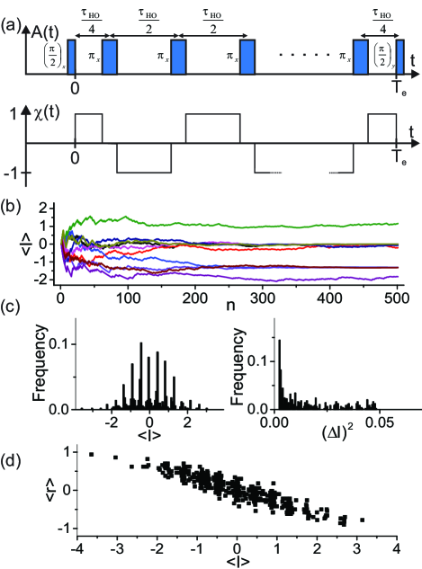
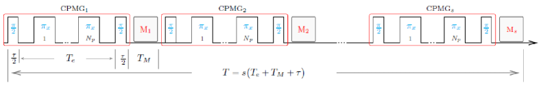
Figure 1: (color online). (a) Pulse sequence (top) used to control the qubit and modulation function for the qubit-HO interaction (bottom). (b) The quadrature average as a function of the measurement step , for a set of simulated trajectories. (c) The distribution of and after measurement steps, extracted from 500 trajectories. (d) The average of qubit readout results over the last 50 points in each measurement trajectory with , versus . In all the simulations .
Measurement protocol.— We consider a system formed of a HO coupled to a qubit, with the Hamiltonian . We have , , , and , with the HO resonance frequency, () Pauli z(x) operators in the qubit energy eigenbasis, the qubit transition frequency, a qubit control term, and the HO-qubit coupling strength. The qubit is controlled with resonant pulses, i.e. by setting , with the amplitude and the phase changing slowly as a function of time. We make a transformation to a rotating frame, described by the unitary operator . In this frame the Hamiltonian is , where we used the rotating wave approximation.
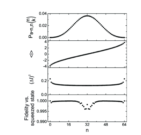
Figure 2: Top three panels: the probability of a measurement sequence with results , the quadrature average, and the quadrature variance, respectively, versus measurement step obtained from Eqs. 1, 2, and 3. Bottom panel: fidelity against a squeezed state versus . We take and .
The measurement protocol consists of repeating the procedure shown schematically in Fig. 1(a). The qubit and the HO start in a separable state , where () is the qubit ground (excited) state and is an arbitrary HO state. Next, the qubit is controlled using a Carr-Purcell-Meiboom-Gill type control sequence Meiboom and Gill (1958), consisting of the pulses , as shown schematically in Fig. 1(a). Each rotation is a rotation of angle around axis or . The first control pulse changes the qubit state to . The evolution of the combined system during the time interval between the initial and final pulses is given by the unitary operator , where the effective Hamiltonian and , the identity operator for the qubit, for for even, and for odd. After the final pulse, the qubit is measured projectively, and the measurement result (), corresponding to projection in the excited (ground) state, is recorded. Following measurement, the qubit is reset to its ground state, in preparation for the next repetition.
The evolution of the coupled qubit-HO system between the two pulses in Fig. 1(a) is exactly described by the Hamiltonian , with the quadrature , obtained by averaging the Hamiltonian over the complete duration of the interaction. Qualitatively speaking, the qubit superposition prepared by the first pulse acquires a phase that depends on the quadrature . The combination of the pulse and measurement in the energy eigenbasis constitutes a measurement in the eigenbasis, which provides information on the quadrature .
Analysis of the measurement process.— Next, we present an analysis of the measurement process. We consider a series of repetitions of the protocol illustrated in Fig. 1(a). For repetition (), the starting state of the combined system is . After interaction and immediately prior to measurement, the state becomes , where and . Here , with the displacement operator of amplitude Walls and Millburn (1995), and . The measurement result () occurs with probability () and induces a post-measurement state (). By iteration, the probability to obtain a set of measurements such that of the results are , is given by and the resulting state is . We note that the probability and the conditioned state are independent of the order in which the results of value are obtained, due to .
We first analyze the measurement action by stochastic numerical simulations. The HO is prepared in its vacuum state. We simulate a set of measurement sequences, each consisting of measurements. Within each sequence, we assign at each step a measurement result , by drawing the random number () with probability (), and we also assign the corresponding conditioned state. In Fig. 1(b) we show, within each sequence, the evolution of the average quadrature versus the measurement step. We observe that after undergoing fluctuations, settles to a nearly constant value. In Fig. 1(c) we show the histogram of the average and of the variance . The distribution of is consistent with the initial state probability, whereas is significantly reduced compared to the initial distribution. These features are a consequence of the quantum non-demolition type of interaction. Remarkably, the values taken by are discrete, a feature that reflects the discrete nature of the information acquired from binary qubit readout results. In Fig. 1(d) we show the average of the last few measurement results versus the final for each sequence. The strong correlation demonstrates that the qubit readout is a suitable meter for the quadrature . The results in Fig. 1 correspond to . We observe similar results for preparation for other values of , with a general tendency for to converge faster and for to decrease as increases. We also observe similar results when the HO is prepared in coherent or thermal states.
We discuss next the properties of the measurement conditioned states. We consider the case in which the initial state of the HO is a coherent state of amplitude . The probability to detect the result for times out of repetitions, the corresponding average, and the corresponding average of the square of the quadrature are given respectively by
(1)
(2)
and
(3)
(see si ).
Using these expressions, we calculate and show in Fig. 2 the probability for each result, which is given by multiplied by the combinatorial factor , the average, and the variance versus . These results show that measurement conditioned states have reduced variance in the quadrature . It is interesting to consider whether the resulting states are squeezed states, as generated by a squeezing operator Walls and Millburn (1995). In Fig. 2 we also show the fidelity of the measurement conditioned state with respect to the state . We find that, besides having reduced variance, the states prepared by measurement have a very high fidelity with respect to states generated by the squeezing operator.
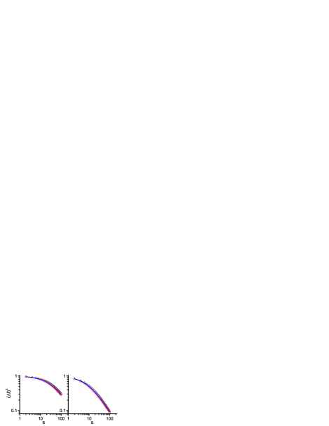
We next consider the dependence of the variance on the number of measurement steps. For an initial vacuum state, the variance of the most likely state () as well as its average weighted over the probabilities of resulting states is shown in Fig. 3 for two values of . Based on equations 1,2, and 3, we derived an analytical approximation for the variance si ,
(4)
which is in excellent agreement with the exact calculations, as shown in Fig. 3.
The role of qubit dephasing.— Given the fact that quadrature measurement relies on the detection of the phase of a qubit superposition, dephasing of a qubit induced by its environment should be considered. In the presence of dephasing, the projection operators become , where is a random phase acquired by the qubit due to noise. The state conditioned by a given series of measurement results , ,…, becomes a density matrix when averaged over noise realizations, and is given by
(5)
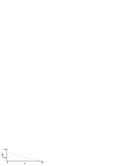
where and are vectors of length with components or , is the sum of the components of , and , with the correlation matrix for the noise . We considered quadrature measurement with MHz, MHz, , and noise in the qubit frequency with a spectral density . This type of noise spectral density is typical in superconducting qubits Bylander et al. (2011); we take a typical value . A comparison of the variance without and with dephasing is shown in Fig. 4. This level of noise produces a negligible effect on quadrature squeezing up to 18. Even with significantly larger noise, , squeezing is degraded by less than 5 %.
Figure 3: (color online). Average variance (triangles) and variance for the symmetric measurement () (dots) versus the number of measurement steps . The solid line is the approximation in Eq. 4. The left and right panels correspond to and respectively.
Experimental implementation.— We briefly discuss the prospects for experimental implementation. We consider a superconducting flux qubit used to measure either an electrical or a mechanical resonator. The flux qubit has GHz, an energy level splitting at the symmetry point , a persistent current nA, an energy relaxation time s, an effective temperature mK, and is subjected to intrinsic flux noise with a spectral density with Orgiazzi et al. (2016); Stern et al. (2014); Yan et al.. The HO has MHz, a quality factor , and a temperature mK. A coupling strength MHz is achievable by inductive coupling of an electrical superconducting resonator or by embedding a moving beam into the qubit arm, similarly to the superconducting interferometer setup in Ref Etaki et al. (2008). With the numbers given above, we find that a HO initially in its thermal state can be brought into a squeezed state with a variance reaching . We note that the assumed value of is conservative. Larger coupling of the qubit to a mechanical HO is envisioned with optimized setups and coupling to an electrical HO can be straightforwardly be made over an order of magnitude larger than considered, leading to larger squeezing. We expect that further optimization of other parameters of the measurement protocol will also result in increased squeezing.
Figure 4: (color online). Variance without noise (crosses) and with noise, with a spectral density (empty dots) and (empty squares) versus the number of measurements.
Conclusions and outlook.— Quadrature measurements and generation of squeezed states are very important in various fields, including quantum sensing, quantum optics, quantum information, and nanomechanics. The protocol for generation of squeezed states that we presented in this paper makes use of a very basic resource, a two level system with control and measurement. This aspect makes it attractive from a fundamental point of view and at the same time amenable to experimental implementations. Future work will address theoretical aspects of optimization of this protocol for optimal squeezing and tests of the experimental implementation.
Acknowledgements.— We thank Martin Otto and Ali Yurtalan for preliminary studies of coupling of a mechanical resonator to a flux qubit, and Aashish Clerk and Eyal Buks for useful discussions. We acknowledge support from Gerald Schwartz and Heather Reisman Foundation, NSERC, Ontario Ministry of Research and Innovation, Industry Canada, and the Canadian Microelectronics Corporation. During part of this work, M.C. was supported for one year by the Scientific and Technological Research Council of Turkey and A.L. was supported by an Ontario Early Research Award.
References
Braginsky and Khalili (1992)V. B. Braginsky and F. Y. Khalili, Quantum
Measurement, edited by K. S. Thorne (Cambridge University Press, 1992).
Taylor et al. (2008)J. M. Taylor, P. Cappellaro,
L. Childress, L. Jiang, D. Budker, P. R. Hemmer, A. Yacoby, R. Walsworth, and M. D. Lukin, Nature Physics 4, 810 (2008) .
Kolkowitz et al. (2012)S. Kolkowitz, A. C. B. Jayich, Q. P. Unterreithmeier, S. D. Bennett, P. Rabl,
J. G. E. Harris, and M. D. Lukin, Science 335, 1603
(2012) .
Bennett et al. (2012)S. D. Bennett, S. Kolkowitz,
Q. P. Unterreithmeier,
P. Rabl, A. C. B. Jayich, J. G. E. Harris, and M. D. Lukin, New Journal of Physics 14, 125004 (2012) .
Bal et al. (2012)M. Bal, C. Deng, J.-L. Orgiazzi, F. Ong, and A. Lupascu, Nat Commun 3, 1324 (2012).
Walls and Millburn (1995)D. F. Walls and G. J. Millburn, Quantum Optics (Springer, 1995).
(27)See supplemental material.
Bylander et al. (2011)J. Bylander, S. Gustavsson, F. Yan,
F. Yoshihara, K. Harrabi, G. Fitch, D. G. Cory, Y. Nakamura, J.-S. Tsai, and W. D. Oliver, Nature Physics 7, 565 (2011) .
Orgiazzi et al. (2016)J.-L. Orgiazzi, C. Deng,
D. Layden, R. Marchildon, F. Kitapli, F. Shen, M. Bal, F. R. Ong, and A. Lupascu, Phys. Rev. B 93, 104518 (2016).
Stern et al. (2014)M. Stern, G. Catelani,
Y. Kubo, C. Grezes, A. Bienfait, D. Vion, D. Esteve, and P. Bertet, Physical review letters 113, 123601 (2014).
(31)F. Yan, S. Gustavsson,
A. Kamal, J. Birenbaum, A. P. Sears, D. Hover, T. J. Gudmundsen, D. Rosenberg, G. Samach, S. Weber, J. L. Yoder, T. P. Orlando, J. Clarke,
A. J. Kerman, and W. D. Oliver, Nature Communications 7, 12964 (2016) .
Etaki et al. (2008)S. Etaki, M. Poot,
I. Mahboob, K. Onomitsu, H. Yamaguchi, and H. S. J. van der Zant, Nature
Physics 4, 785 (2008) .
Supplementary material: Quadrature readout and generation of squeezed states of a harmonic oscillator using a qubit-based indirect measurement
I Derivation of the expressions for probability, quadrature average and variance
In this section we present a derivation of the expressions for , , and in Eqs. (1)–(3) of the main text. The probability to obtain results in a series of measurement is , with the initial harmonic oscillator (HO) state, taken to be a coherent state of complex amplitude . We have , where we used , , and . Using the binomial theorem, this expression can be expanded as
(S1)
When the last factor in (S1) in the bra-ket notation is expanded further by employing the formulas and Walls and Millburn (1995), the expression for given in Eq. (1) of the main text is obtained.
The quadrature average . Using the relations above and , we obtain . This is expanded as
(S2)
After using , equation (S2) yields the final form of in the main text.
Similarly, we can expand as
(S3)
Using , we can obtain the final form of in Eq.(3).
We can establish the following relation between the probability, quadrature average, and quadrature square average:
(S4)
This relation will be used in the following section.
II derivation of an approximate formula for the variance
In this section we derive an expression for the quadrature variance. We assume a starting vacuum state, and we focus on ( is taken even), which is the most likely result. We have
(S5)
where
(S6)
The function is maximum at and symmetric around (i.e. with ). We have:
(S7)
The combinatorial factor in (S7) is well described by normal approximation Rosen (2001),
(S8)
if is not much larger than .
With (S8), equation (S5) becomes
(S9)
where .
The sum in (S9) is well approximated in the limit by the Jacobi theta function: which is approximated as
for .
The final form of the asymptotic probability becomes
(S10)
Using Eq. (S4) for and noting that , the variance becomes
(S11)
which is result (4) in the main text.
III Models for decoherence
III.1 Pure dephasing due to flux noise
For a superconducting flux qubit, flux noise is the dominant source of dephasing. In the energy eigenbasis, the Hamiltonian of the qubit is
(S12)
where , with the so-called qubit gap and , with , where is the externally applied magnetic flux and is the magnetic flux quantum, and the qubit persistent current Orlando et al. (1999). The term is a random component induced by intrinsic fluctuations of magnetic flux.
The random component in (S12) is a stochastic process, which can be written as
(S13)
where , with , where is a time taken much longer than the duration of the simulated experiment (see Fig. S1). The coefficients are taken as random Gaussian variables.
Figure S1: Quadrature detection using the qubit. Each in this schema is represented in Fig. 1.a in the main text.
The low frequency noise process is characterized by power spectral density (PSD) where , where the PSD of flux noise is assume to be .
We assume and nA, typical for a flux qubit. For simulations of noise trajectories, we restrict the noise frequency to the range
where and with and are taken sufficiently large to reflect the relevant time scales and is number of pulses.
We construct noise trajectories by using randomly generated complex Fourier coefficients , related to the PSD by
.
III.2 Dissipative effects in the coupled system
We model decoherence of the coupled qubit-harmonic oscillator system using the master equation in Lindblad form:
(S14)
where is the density matrix, is the Hamiltonian, is the
damping factor defined by a mapping
In equation (S14), and are the decay rates with average photon number at frequency and a finite temperature ( is the Boltzmann constant)
and is the decay rate of the resonator with a quality factor Gardiner and Zoller (2000). Besides, and
are decay rates for the qubit at a finite temperature with
and is the relaxation time;
is the pure dephasing rate.
The Hamiltonian that governs the master equation (S14) is given by
(S15)
where
with is given in (S13).
In this study, we omitted the influence of the last term in (S14) by setting ,
since the flux noise is the dominant source of dephasing and its contribution is embedded into the Hamiltonian (S15).
IV Derivation of conditional evolution with pure dephasing
With pure dephasing, a random phase is added to a qubit superposition, which has a different value for each repetition from to . The noise is drawn from a proper distribution corresponding to the noise spectrum and taking into account the noise modulation due to the CPMG sequence (Fig. S1).
Using the projection operator and following the procedure in the main text, one can obtain pure state conditioned on measurement result :
(S16)
where is the initial state,
is a vector of length with components (), is the vector of length formed of the values of the random phase (),and
.
Consequently, the density matrix in the main text is obtained
from (S16) by averaging over the noise process:
(S17)
where with
the correlation matrix for the noise .
The correlation matrix can be written as
(S18)
where is Fourier transform of depicted in Fig. 1.(a) in the main text. We find that to a good approximation, the correlation matrix (S18) is diagonal, with elements
(S19)
References
Walls and Millburn (1995)D. F. Walls and G. J. Millburn, Quantum Optics (Springer, 1995) .
Rosen (2001)K. H. Rosen, Handbook of discrete and
combinatorial mathematics, 2nd ed., Springer Study
Edition (CRC press, 2001).
Orlando et al. (1999)T. P. Orlando, J. E. Mooij,
L. Tian, C. H. van der Wal, L. S. Levitov, S. Lloyd, and J. J. Mazo, Phys. Rev. B 60, 15398 (1999).
Gardiner and Zoller (2000)C. Gardiner and P. Zoller, Quantum Noise: A
Handbook of Markovian and Non-Markovian Quantum Stochastic Methods With
Applications to Quantum Optics (Springer
Verlag, 2000).