Penguin pollution in $\beta$ and $\beta_{s}$

Abstract:

The mixing-induced CP asymmetries in $B_{d}\to J/\psi K_{S}$ and $B_{s}\to J/\psi\phi$ are essential to detect or constrain new physics in the $B_{d}\!-\overline{\!B}{}_{d}$ and $B_{s}\!-\overline{\!B}{}_{s}$ mixing amplitudes, respectively. To this end one must control the penguin contributions to the decay amplitudes, which affect the extraction of fundamental CP phases from the measured CP asymmetries. Although the “penguin pollution” is doubly Cabibbo-suppressed, it could compete in size with current experimental errors. In this talk I present a calculation of the penguin contributions treating QCD effects with soft-collinear factorisation and compare method and results with the alternative approach employing flavour-SU(3) symmetry. As a novel feature, I present results for the penguin pollution in $b\to c\overline{c}d$ modes.

1 Introduction

In this talk I discuss time-dependent CP asymmetries

$$A_{\rm CP}^{B_{q}\to f}(t)\equiv\frac{\Gamma(\,\overline{\!B}_{q}(t)\to f)-\Gamma(B_{q}(t)\to f)}{\Gamma(\,\overline{\!B}_{q}(t)\to f)+\Gamma(B_{q}(t)\to f)},\qquad\qquad q=d\mbox{ or }s,$$ (1)

for $B_{d,s}$ decays into final states $f$ consisting of a charmonium and a light pseudoscalar or vector boson. Prime examples are the decays $B_{d}\to J/\psi K_{S}$ and $B_{s}\to J/\psi\phi$, which are both triggered by the quark decay $\overline{b}\to\overline{c}c\overline{s}$. I only consider the case that $f$ is a CP eigenstate; if $f$ comprises two vector mesons (as in $B_{s}\to J/\psi\phi$) it is understood that the CP-even and CP-odd components are properly separated through an angular analysis. Precise measurements of these mixing-induced CP asymmetries serve to determine the CP phases related to the $B_{d}\!-\overline{\!B}{}_{d}$ and $B_{s}\!-\overline{\!B}{}_{s}$ mixing amplitudes. Within the Standard Model these are

$$2\beta\equiv\arg\left(\frac{V_{tb}V_{td}^{*}}{V_{cb}V_{cd}^{*}}\right)^{2}\qquad \;\mbox{and}\qquad 2\beta_{s}\equiv\arg\left(\frac{V_{tb}^{*}V_{ts}}{V_{cb}^{*}V_{cs}}\right)^{2}.$$ (2)

Here $(V_{tb}V_{tq}^{*})^{2}$ stems from the box diagrams shown in Fig. 1. The $B_{q}\!-\overline{\!B}{}_{q}$ mixing amplitudes probe virtual effects of new particles with masses as high as 100 TeV, if new physics enters $B_{q}\!-\overline{\!B}{}_{q}$ mixing at tree level. It is therefore of utmost importance to control the theoretical uncertainties in the relation between the measured $A_{\rm CP}^{B_{q}\to f}(t)$ and the fundamental CP phases in Eq. (2) as precisely as possible.

Figure 1: Box diagrams describing $B_{d}\!-\overline{\!B}{}_{d}$ and $B_{s}\!-\overline{\!B}{}_{s}$ mixing in the Standard Model.

 

The CP asymmetry in Eq. (1) reads

$$A_{\rm CP}^{B_{q}\to f}(t)=\frac{S_{f}\sin(\Delta m_{q}t)-C_{f}\cos(\Delta m_{q}t)}{\cosh(\Delta\Gamma_{q}t/2)+A_{f,\Delta\Gamma_{q}}\sinh(\Delta\Gamma_{q}t/2)}.$$ (3)

Here $\Delta m_{q}$ and $\Delta\Gamma_{q}$ are the mass and width difference, respectively, between the mass eigenstates of the $B_{q}\!-\overline{\!B}{}_{q}$ system. $\Delta m_{q}$ and $\Delta\Gamma_{q}$ are CP-conserving quantities calculated from the box diagrams in Fig. 1. In $B_{d}$ decays we can set the denominator in Eq. (3) to 1, because $\Delta\Gamma_{d}$ is very small. The coefficients $S_{f}$, $C_{f}$, and $A_{f,\Delta\Gamma_{q}}$ depend on the decay amplitude $A(B_{q}\to f)$. For the $\overline{b}\to\overline{c}c\overline{s}$ amplitudes of interest one usually writes:

$$A(B_{q}\to f)=V_{cb}^{*}V_{cs}T_{f}+V_{ub}^{*}V_{us}P_{f}.$$ (4)

The “tree” and “penguin” amplitudes read

$$T_{f} = \frac{G_{F}}{\sqrt{2}}\langle f|C_{1}Q_{1}^{c}+C_{2}Q_{2}^{c}+\sum_{j}C_{j}Q_{j}|B_{q}\rangle,$$ (5)

$$P_{f} = \frac{G_{F}}{\sqrt{2}}\langle f|C_{1}Q_{1}^{u}+C_{2}Q_{2}^{u}+\sum_{j}C_{j}Q_{j}|B_{q}\rangle.$$ (6)

Here $G_{F}$ is the Fermi constant and $Q_{1}^{q}=\overline{q}{}^{\alpha}\gamma_{\mu}(1-\gamma_{5})s^{\beta}\overline{b}{}^{\beta}\gamma^{\mu}(1-\gamma_{5})q^{\alpha}$ and $Q_{2}^{q}=\overline{q}{}^{\alpha}\gamma_{\mu}(1-\gamma_{5})s^{\alpha}\overline{b}{}^{\beta}\gamma^{\mu}(1-\gamma_{5})q^{\beta}$ are the current-current operators generated by $W$-boson exchange. The sum over $j$ comprises the penguin operators $Q_{3-6}$ and the chromomagnetic operator $Q_{8G}$ (see Ref. [1] for the definitions). The $C_{k}$’s are the Wilson coefficients which encode the short-distance physics; the top-quark penguin loops (entering $C_{3-6}$ and $C_{8G}$) appear in both $T_{f}$ and $P_{f}$, because the CKM unitarity relation $V_{tb}^{*}V_{ts}=-V_{cb}^{*}V_{cs}-V_{ub}^{*}V_{us}$ is used to eliminate $V_{tb}^{*}V_{ts}$ from Eq. (6). Expanding to first order in $\epsilon=|V_{us}V_{ub}/(V_{cs}V_{cb})|\approx 0.02$ one has

$$S_{f}\simeq-\eta_{f}\sin(\phi_{q}+\Delta\phi_{q}) \qquad\quad\mbox{with~{}~{}~{}~{}~{}~{}~{}}\tan(\Delta\phi_{q})\simeq\;2\epsilon\sin\gamma\;{\rm Re}\,\frac{P_{f}}{T_{f}},$$ (7)

where $C\!P\ \!|f\rangle=\eta_{f}|f\rangle$ with $\eta_{f}=\pm 1$, $\phi_{d}=2\beta$, and $\phi_{s}=-2\beta_{s}$. Furthermore, $C_{f}\simeq 2\epsilon\sin\gamma\,{\rm Im}\,(P_{f}/T_{f})$ quantifies direct CP violation.

$\Delta\phi_{q}$ in Eq. (7) is the penguin pollution which obscures a clean extraction of $\phi_{q}$ from the measured $S_{f}$. The size of the penguin pollution depends on the considered decay mode through ${\rm Re}\,(P_{f}/T_{f})$ in Eq. (7). A standard way to estimate $\Delta\phi_{q}$ employs the flavour-SU(3) symmetry of QCD or its SU(2) subgroup U-spin. The latter connects pairs of hadronic matrix elements related by the interchange of down and strange quarks. In the case of $B_{d}\to J/\psi K_{S}$ one can extract the desired $P_{f}/T_{f}$ from control channels such as $B_{s}\to J/\psi K_{S}$ or $B_{d}\to J/\psi\pi^{0}$, which are induced by the quark decay $\overline{b}\to\overline{c}c\overline{d}$. In these control channels the CKM factor $\epsilon$ is replaced by $|V_{ud}V_{ub}/(V_{cd}V_{cb})|\approx 0.38$ which permits to determine $P_{f}/T_{f}$ from the coefficients $C_{f}$ and $S_{f}$ measured in these modes. In this way one finds the values $-3.9^{\circ}\leq\Delta\phi_{d}\leq-0.8^{\circ}$ [2], $|\Delta\phi_{d}|\leq 1.6^{\circ}$ [3], $|\Delta\phi_{d}|\leq 0.8^{\circ}$ [4], and $\Delta\phi_{d}=-1.1^{\circ}\raisebox{-2.15277pt}{\shortstack[l]{$\scriptstyle+0.85^{\circ}$\\ $\scriptstyle-0.7^{\circ}$}}$ [5] for $f=J/\psi K_{S}$. The values (listed in chronological order) become more accurate with more precise data the on the control channels. A general drawback of the method is the unknown size of SU(3)_f breaking caused by unequal strange and down quark masses. SU(3)_f symmetry can be very accurate, as e.g. in semileptonic $B_{d,s}$ decays, but may also fail completely: for example, a $b$ quark fragments into a $B_{d}$ meson almost four times more often than into a $B_{s}$. In the case of $B_{s}\to J/\psi\phi$ one faces the problem that the $\phi$ meson is an equal mixture of an octet and a singlet of SU(3)_f symmetry. It is not clear how to treat SU(3)_f breaking in such a case of maximal symmetry violation and the method may fail in this case.

The experimental world average $2\beta+\Delta\phi_{d}=43.8^{\circ}\pm 1.4^{\circ}$ [7] is dominated by $B_{d}\to J/\psi K_{S}$, so that $\Delta\phi_{d}$ here can be identified with the penguin pollution in this mode. The experimental error is comparable in size with the expected penguin pollution. The situation is similar with the experimental value $2\beta_{s}+\Delta\phi_{s}=1.7^{\circ}\pm 1.9^{\circ}$ [7] which dominantly stems from LHCb data on $B_{s}\to J/\psi K^{+}K^{-}$ and $B_{s}\to J/\psi f_{0}[\to\pi^{+}\pi^{-}]$, with an experimental error of $2.2^{\circ}$ on $2\beta_{s}+\Delta\phi_{s}$ [9]. The statistical powers of $B_{s}\to J/\psi\phi[\to K^{+}K^{-}]$, non-resonant $B_{s}\to J/\psi K^{+}K^{-}$, and $B_{s}\to J/\psi f_{0}[\to\pi^{+}\pi^{-}]$ on the determination of $2\beta_{s}+\Delta\phi_{s}$ are 52%, 8%, and 42%, respectively [10]. The value of $2\beta_{s}$ inferred from a global fit to the CKM unitarity triangle is $2\beta_{s}=2.12^{\circ}\pm 0.04^{\circ}$ [8].

In this talk I present calculations of the penguin contributions to CP asymmetries which do not use SU(3)_F symmetry, but instead employ soft-collinear factorisation in QCD [6].

2 Operator Product Expansion

Many physical problems involve a hard scale $\sqrt{q^{2}}$ which is much larger than the fundamental scale $\Lambda_{\rm QCD}\sim 0.4\,\mbox{GeV}$ of QCD. The operator product expansion (OPE) is a calculational tool to express the quantity of interest in terms of a series in $\Lambda_{\rm QCD}/\sqrt{q}$. In our case we a apply the OPE to $P_{f}$ in Eq. (6) and $\sqrt{q^{2}}\sim m_{\psi}\sim 3\,\mbox{GeV}$ is the hard scale. The troublesome contribution to $P_{f}$ stems from $Q_{1,2}^{u}$ in Eq. (6); the corresponding one-loop contribution is shown in Fig. 2. The OPE for the contribution of $Q_{j}^{u}$, $j=1,2$, to $P_{f}$ for $B_{d}\to J/\psi K_{S}$ reads

$$\!\!\langle J/\psi K_{S}|Q_{j}^{u}|B_{d}\rangle = \sum_{k}\widetilde{C}_{j,k}\langle J/\psi K_{S}|Q_{k}|B_{d}\rangle+\ldots$$ (8)

Here $k=0V,0A,8V,8A$ labels different local four-quark operators with flavour structure $\overline{b}s\,\overline{c}c$:

$$Q_{0V} \equiv \overline{b}{}\gamma_{\mu}(1-\gamma_{5})s\,\overline{c}{}\gamma^{\mu}c,$$

$$Q_{0A} \equiv \overline{b}{}\gamma_{\mu}(1-\gamma_{5})s\,\overline{c}{}\gamma^{\mu}\gamma_{5}c,$$

$$Q_{8V} \equiv \overline{b}{}\gamma_{\mu}(1-\gamma_{5})T^{a}s\,\overline{c}{}\gamma^{\mu}T^{a}c,$$

$$Q_{8A} \equiv \overline{b}{}\gamma_{\mu}(1-\gamma_{5})T^{a}s\,\overline{c}{}\gamma^{\mu}\gamma_{5}T^{a}c.$$ (9)

These operators suffice to reproduce $P_{f}$ at the leading power of $\Lambda_{\rm QCD}/\sqrt{q}$. Sub-leading powers involve additional operators , which are indicated by the dots in Eq. (8). The Wilson coefficients $\widetilde{C}_{j,k}$ in Eq. (8) are found by calculating $\overline{b}\to\overline{c}c\overline{s}$ Feynman diagrams with $Q_{j}^{u}$ in the desired order of $\alpha_{s}$ and comparing the result with Feynman diagrams involving the operators $Q_{k}$ in Eq. (9) in the corresponding order of QCD. The leading non-vanishing order, shown in Fig. 2, only involves the operator $Q_{8V}$ on the right-hand side (RHS) of the OPE in Eq. (8).

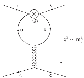
$$q^{2}\gg\Lambda_{QCD}^{2}$$

        $\displaystyle\longrightarrow$

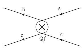
Figure 2: Pictorial representation of the OPE for the up-quark loop: Since the momentum transfer $q$ to the charmonium is large, we can express the left diagram as the product of a perturbative Wilson coefficient and the effective four-quark operator on the right.

 

The coefficient is

$$\widetilde{C}_{2,8V}^{(0)} = \frac{2}{3}\frac{\alpha_{s}}{4\pi}\left[\ln\left(\frac{q^{2}}{\mu^{2}}\right)-i\pi-\frac{2}{3}\right],$$ (10)

where $\mu$ is the renormalisation scale. The idea to factorise the one-loop diagram in this way was proposed by Bander, Silverman, and Soni (BSS) in Ref. [11] and applied to $B_{d}\to J/\psi K_{S}$ in Ref. [12]. In order to establish the OPE in Eq. (8) one must prove that the coefficients $\widetilde{C}_{j,k}$ are free from infrared singularities, which involves the study of higher orders in $\alpha_{s}$. This proof has been carried out in Ref. [6] and involves the analysis of (i) soft IR divergences of the two-loop diagrams contributing to $\langle Q_{j}^{u}\rangle$, (ii) collinear IR divergences of these diagrams, (iii) spectator scattering diagrams, and (iv) higher-order diagrams in which the large momentum bypasses the penguin loop (“long distance penguins”). Sample diagrams are shown in Fig. 3.

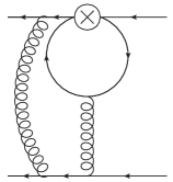
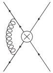
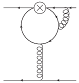
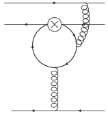
Figure 3: The soft IR divergence of the first diagram (contributing to the LHS of Eq. (8)) factorises with the corresponding diagram of the local operator (RHS of Eq. (8)) shown next. The third diagram has a collinear IR divergence and finally a spectator-scattering diagram is shown.

 

In Ref. [6] it has been shown that indeed all infrared singularities properly factorise and cancel from the coefficients $\widetilde{C}_{j,k}$, which therefore can be calculated perturbatively order-by-order in $\alpha_{s}$. The leading order (LO) contribution to the $\widetilde{C}_{j,k}$ stems from the penguin operators $Q_{3-6}$ in Eq. (6), which contribute trivially to Eq. (8) as local $\overline{b}s\,\overline{c}c$ operators. The dependence of $C_{3-6}$ on the unphysical renormalisation scale $\mu$ cancels (to order $\alpha_{s}$) with the $\mu$-dependent terms of the next-to-leading order (NLO) corrections. The result in Eq. (10) belongs to the NLO and depends on the renormalisation scale and scheme. It is only meaningful in combination with the LO contributions involving $C_{3-6}$, so that these scale and scheme dependences cancel. In Ref. [12] the LO contribution has been omitted and the inferred penguin pollution is substantially smaller than the one found by us.

The standard application of soft-collinear factorisation in flavour physics addresses $B$ decays into two light mesons (QCD factorisation) [13]. In our case instead one of the final-state mesons is heavy and the $J/\psi$ mass is the relevant heavy scale in the problem. As a consequence, we cannot factorise the matrix element of colour-octet four-quark operators into a form factor and a decay constant [14].

3 Matrix elements and numerical results

In order to predict the size of the penguin pollution $\Delta\phi_{d}$ for $B_{d}\to J/\psi K_{S}$ in Eq. (7) from the calculated ${\rm Re}\,(P_{f}/T_{f})$ we need the (ratios of the) hadronic matrix elements

$$v_{0}V_{0}\equiv\langle J/\psi K^{0}|Q_{0V}|B_{d}\rangle, \qquad a_{0}V_{0}\equiv\langle J/\psi K^{0}|Q_{0A}|B_{d}\rangle,$$

$$v_{8}V_{0}\equiv\langle J/\psi K^{0}|Q_{8V}|B_{d}\rangle, \qquad a_{8}V_{0}\equiv\langle J/\psi K^{0}|Q_{8A}|B_{d}\rangle.$$ (11)

Eq. (11) defines the complex parameters $v_{0,8}$ and $a_{0,8}$ with the common normalisation factor

$$V_{0}\equiv\;\langle J/\psi K^{0}|Q_{0V}|B_{d}\rangle_{\rm fact}=\;2f_{J/\psi}m_{B_{d}}p_{cm}F_{1}^{B\to K}(m_{\psi}^{2})=\;(4.26\pm 0.16)\,\mbox{GeV}{}^{3}.$$ (12)

$V_{0}$ is the factorised matrix element of the colour-singlet operator $Q_{0V}$ involving the $J/\psi$ decay constant $f_{J/\psi}$, the $B_{d}$ mass $m_{B_{d}}$, the magnitude of the $K_{S}$ center-of mass three-momentum $p_{cm}$, and the form factor $F_{1}^{B\to K}$. Next $v_{0,8}$ and $a_{0,8}$ are categorised in terms of $1/N_{c}$ counting, where $N_{c}=3$ is the number of colours. One has $v_{0}=1+{\cal O}(1/N_{c}^{2})$, $v_{8},a_{8}={\cal O}(1/N_{c})$, and $a_{0}={\cal O}(1/N_{c}^{2})$. It is well-known that the coefficient of $v_{0}$ in $T_{f}$ is small, so that the branching ratio $B(B_{d}\to J/\psi K_{S})$ is dominated by $v_{8}$ and $a_{8}$. Therefore we can use the measured $B(B_{d}\to J/\psi K_{S})_{\rm exp}$ as a cross-check of our colour counting for the peculiar colour-octet matrix elements. With the numerical values of the Wilson coefficients and Eq. (12) one finds [6]:

$$\frac{B(B_{d}\to J/\psi K_{S})}{B(B_{d}\to J/\psi K_{S})_{\rm exp}} = \left[1\pm 0.08\right]\left|0.47v_{0}+7.8(v_{8}-a_{8})\right|^{2}.$$ (13)

This implies $0.07\leq|v_{8}-a_{8}|\leq 0.19$ if $v_{0}$ is set to 1, illustrating that the colour counting works for the branching ratio. $a_{0}$ comes with small coefficients in both $T_{f}$ and $P_{f}$ and is negligible. For the prediction of $P_{f}/T_{f}$ at NLO we need $v_{8}$ and impose $|v_{8}|\leq 1/3$, complying with colour counting, and vary the phases of the matrix elements between $-\pi$ and $\pi$. The result is [6]

$$|\Delta_{d}|\leq 0.68^{\circ},\qquad\quad|C_{J/\psi K_{S}}|\leq 1.33\cdot 10^{-2}.$$ (14)

The bound on $\Delta_{d}$ is comparable to the one derived from SU(3)_F symmetry (quoted in the introduction), but sharper.

In the case of $B_{s}\to J/\psi\phi$ one finds

$\displaystyle(J/\psi\phi)^{0}$	$\displaystyle(J/\psi\phi)^{\parallel}$	$\displaystyle(J/\psi\phi)^{\perp}$
$\displaystyle|\Delta\phi_{s}|\leq 0.97^{\circ}$	$\displaystyle|\Delta\phi_{s}|\leq 1.22^{\circ}$	$\displaystyle|\Delta\phi_{s}|\leq 0.99^{\circ}$
$\displaystyle|C_{f}|\leq 1.89\cdot 10^{-2}$	$\displaystyle|C_{f}|\leq 2.35\cdot 10^{-2}$	$\displaystyle|C_{f}|\leq 1.92\cdot 10^{-2}$

for the scalar, parallel, and perpendicular polarisation states, respectively.

As a novel feature, the method of Ref. [6] permits the prediction of the penguin contributions to $\overline{b}\to\overline{c}c\overline{d}$ decays, for example:

$$B_{d}\to J/\psi\pi^{0}:\qquad \quad|S_{J/\psi\pi^{0}}+\sin(2\beta)|\leq 0.18,\qquad|C_{J/\psi\pi^{0}}|\leq 0.29.\qquad$$ (15)

$$B_{s}\to J/\psi K_{S}:\qquad |S_{J/\psi K_{S}}-\sin(-2\beta_{s})|\leq 0.26,\qquad|C_{J/\psi K_{S}}|\leq 0.27.\qquad$$ (16)

The first result means $-0.86\leq S_{J/\psi\pi^{0}}\leq-0.50$. Eq. (15) favours the Belle result [15] $S_{J/\psi\pi^{0}}=-0.67\pm 0.22$, $C_{J/\psi\pi^{0}}=-0.08\pm 0.17$ over the BaBar result [16] $S_{J/\psi\pi^{0}}=-1.23\pm 0.21$, $C_{J/\psi\pi^{0}}=-0.20\pm 0.19$. Predictions for more $\overline{b}\to\overline{c}c\overline{s}$ and $\overline{b}\to\overline{c}c\overline{d}$ modes can be found in Tab. 1 of Ref. [6].

It is worthwhile to compare the methods and results presented in this talk with those of the alternative approach based on SU(3)_F symmetry: It is gratifying to see that the two completely different methods give compatible results for $\Delta\phi_{d}$ in the case of $B_{d}\to J/\psi K_{S}$. However, the SU(3)_F estimate of $\Delta\phi_{d}$ depends on the choice for the size of SU(3)_F breaking added to the value of $P_{f}/T_{f}$ extracted from the $\overline{b}\to\overline{c}c\overline{d}$ control channels. In analyses of branching fractions (which probe $T_{f}$ with little sensitivity to $P_{f}$) it is possible to include linear SU(3)_F breaking in the $T_{f}$ amplitudes and thereby test the quality of the method from the data (see Ref. [4] for $B\to J/\psi X$ decays and Refs. [18] and [17] for $B,D$ decays to two light mesons, respectively). However, in the case of the up-quark loop in $P_{f}$ there is not enough information to disentangle the penguin pollution from the matrix elements parametrising SU(3)_F breaking, no matter how many control channels are included: The SU(3)_F breaking stemming from the $d\to s$ replacement when linking the $\overline{b}\to\overline{c}c\overline{d}$ control channel to the $\overline{b}\to\overline{c}c\overline{s}$ signal process is never constrained by any of these control channel processes. On the contrary, the OPE-based approach of Ref. [6] makes enough redundant predictions to simultaneously test the method and to constrain the penguin pollution in the $\overline{b}\to\overline{c}c\overline{s}$ decays: Here the litmus test are the predictions for the various $\overline{b}\to\overline{c}c\overline{d}$ channels (such as those in Eqs. (15) and (16)), which make the method falsifiable.

The SU(3)_F method utilises the feature that the SU(3)_F symmetry is approximately exact, with corrections treatable as small (i.e. ${\cal O}(30\%)$) perturbations. The quality of the symmetry allows us to assign exact or approximate SU(3)_F quantum numbers to the particle states, as we routinely do for the light pseudoscalar mesons. In the case of $B_{s}\to J/\psi\phi$ one faces the fact that the $\phi$ meson is an equal mixture of octet and singlet, so that it does not correspond to an approximate SU(3)_F eigenstate. There are two possible explanations of this observations: (i) SU(3)_F is not a good symmetry for decays into final states with vector mesons. (ii) SU(3)_F breaking is small, but the spectrum of the “unperturbed” strong hamiltonian (corresponding to the limit $m_{s}=m_{d}=m_{u}$) is almost degenerate, so that even a small perturbation can lead to maximal mixing. If case (i) is realised in nature, SU(3)_F cannot be applied to constrain the penguin pollution in $B_{s}\to J/\psi\phi$. If (ii) is the correct explanation, a necessary ingredient of an SU(3)_F-based assessment of the penguin pollution is the determination of both the octet and singlet matrix elements from the control channels. In addition, one must develop a formalism which permits the treatment of SU(3)_F breaking for the case that the final states of the considered decays cannot be approximated by SU(3)_F eigenstates. In view of this situation it is safe to say that SU(3)_F-based estimates of the penguin pollution in $B_{s}\to J/\psi\phi$ rest on shaky ground.

4 Conclusions and outlook

In this talk I have presented results of Ref. [6] for the penguin pollution affecting the extractions of the CP phases $2\beta$ and $2\beta_{s}$ from the decays $B_{d}\to J/\psi K_{S}$ and $B_{s}\to J/\psi\phi$, respectively. The predictions are based on a new calculational approach which utilises an operator product expansion (OPE) for the penguin amplitude. To establish the OPE the infrared safety of the Wilson coefficients calculated from the up-quark loop contribution to the penguin amplitude had to be proven, which elevates the BSS approach of Ref. [11] to a field-theoretic concept applicable at any order of $\alpha_{s}$. (However, we found no justification to apply the OPE to the charm-quark loop, which in our framework resides in the hadronic matrix elements.) Our method can also be applied to CP asymmetries in $\overline{b}\to\overline{c}c\overline{d}$ decays, in which the penguin-to-tree ratio is much larger. As examples I have quoted bounds on the penguin contributions for the CP asymmetries in the decays $B_{d}\to J/\psi\pi^{0}$ and $B_{s}\to J/\psi K_{S}$. The confrontation of our predictions for $\overline{b}\to\overline{c}c\overline{d}$ decays with more precise data will be a stringent test of the OPE-based approach. In the future the errors of the predictions may shrink, if effort is put into the calculation of the hadronic parameter $v_{8}$, possibly with the help of QCD sum rules. In my talk I have further expressed a critical view of the application of SU(3)_F symmetry to the penguin pollution in $B_{s}\to J/\psi\phi$.

References

- [1] G. Buchalla, A. J. Buras and M. E. Lautenbacher, Rev. Mod. Phys. 68, 1125 (1996) [hep-ph/9512380].
- [2] S. Faller, M. Jung, R. Fleischer and T. Mannel, Phys. Rev. D 79 (2009) 014030 doi:10.1103/PhysRevD.79.014030 [arXiv:0809.0842 [hep-ph]].
- [3] M. Ciuchini, M. Pierini and L. Silvestrini, arXiv:1102.0392 [hep-ph].
- [4] M. Jung, Phys. Rev. D 86 (2012) 053008 doi:10.1103/PhysRevD.86.053008 [arXiv:1206.2050 [hep-ph]].
- [5] K. De Bruyn and R. Fleischer, JHEP 1503 (2015) 145 doi:10.1007/JHEP03(2015)145 [arXiv:1412.6834 [hep-ph]].
- [6] P. Frings, U. Nierste and M. Wiebusch, Phys. Rev. Lett. 115 (2015) no.6, 061802 doi:10.1103/PhysRevLett.115.061802 [arXiv:1503.00859 [hep-ph]].
- [7] Heavy Flavor Averaging Group, summer 2016 data, www.slac.stanford.edu/xorg/hfag/triangle/summer2016.
- [8] A. Höcker, H. Lacker, S. Laplace and F. Le Diberder [CKMfitter Group], Eur. Phys. J. C 21 (2001) 225 doi:10.1007/s100520100729 [hep-ph/0104062], update of December 2016, http://ckmfitter.in2p3.fr/www/results/plots_ichep16/ckm_res_ichep16.html.
- [9] R. Aaij et al. [LHCb Collaboration], Phys. Rev. D 87 (2013) no.11, 112010 doi:10.1103/PhysRevD.87.112010 [arXiv:1304.2600 [hep-ex]]. R. Aaij et al. [LHCb Collaboration], Phys. Rev. Lett. 114 (2015) no.4, 041801 doi:10.1103/PhysRevLett.114.041801 [arXiv:1411.3104 [hep-ex]]. R. Aaij et al. [LHCb Collaboration], Phys. Lett. B 736 (2014) 186 doi:10.1016/j.physletb.2014.06.079 [arXiv:1405.4140 [hep-ex]].
- [10] Stephanie Hansmann-Menzemer, private communication.
- [11] M. Bander, D. Silverman and A. Soni, Phys. Rev. Lett. 43, 242 (1979).
- [12] H. Boos, T. Mannel and J. Reuter, Phys. Rev. D 70, 036006 (2004) [hep-ph/0403085].
- [13] M. Beneke, G. Buchalla, M. Neubert and C. T. Sachrajda, Phys. Rev. Lett. 83, 1914 (1999) [hep-ph/9905312]; Nucl. Phys. B 591, 313 (2000) [hep-ph/0006124].
- [14] J. Chay and C. Kim, hep-ph/0009244. M. Beneke, Nucl. Phys. Proc. Suppl. 111, 62 (2002) [hep-ph/0202056].
- [15] S. E. Lee et al. [Belle Collaboration], Phys. Rev. D 77, 071101 (2008) [arXiv:0708.0304 [hep-ex]].
- [16] B. Aubert et al. [BaBar Collaboration], Phys. Rev. Lett. 101, 021801 (2008) [arXiv:0804.0896 [hep-ex]].
- [17] S. Müller, U. Nierste and S. Schacht, Phys. Rev. D 92 (2015) no.1, 014004 doi:10.1103/PhysRevD.92.014004 [arXiv:1503.06759 [hep-ph]].
- [18] M. Gronau, O. F. Hernandez, D. London and J. L. Rosner, Phys. Rev. D 52 (1995) 6356 doi:10.1103/PhysRevD.52.6356 [hep-ph/9504326].