Deep Kernel Recursive Least-Squares Algorithm

Abstract

We present a new kernel-based algorithm for modeling evenly distributed multidimensional datasets that does not rely on input space sparsification. The presented method reorganizes the typical single-layer kernel-based model into a deep hierarchical structure, such that the weights of a kernel model over each dimension are modeled over its adjacent dimension. We show that modeling weights in the suggested structure leads to significant computational speedup and improved modeling accuracy.

1 Introduction

Many natural and man-made phenomena are distributed over large spatial and temporal scales. Some examples include weather patterns, agro-ecological evolution, and social-network connectivity patterns. Modeling such phenomena has been the focus of research during the past decades Tryfona ; Vedula . Of the many techniques studied, Kernel methods Bishop , have emerged as a leading tool for data-driven modeling of nonlinear spatiotemporally varying phenomena. Kernel-based estimators with recur.sive least squares (RLS) (or its sparsified version) learning algorithms represent the state-of-the-art in data-driven spatiotemporal modeling Sliding ; NORMA ; Fixed ; KRLST ; QKLMS ; TLAF ; GARCIAVEGA2019 . However, even with the successes of these algorithms, modeling of large datasets with significant spatial and temporal evolution remains an active challenge. As the size of the dataset increases, the number of kernels that needs to be utilized begins to increase. This consequently leads to a large kernel matrix size and computational inefficiency of the algorithm Engel . The major stream of thought in addressing this problem has relied on the sparsification of the kernel dictionary in some fashion. In the time-invariant case, the Kernel Recursive Least-Squares method (KRLS) scales as $\mathcal{O}(m^{2})$, where $m$ is the size of the kernel dictionary. Now suppose our dataset is varying with time, and we add time as the second dimension. Then KRLS cost scales as $\mathcal{O}((mm_{1})^{2})$, where $m_{1}$ is the number of time-steps. While sparsification can reduce the size of $m$ and $m_{1}$ to some extent, it is easy to see that as the dimension of the input space increases, the computational cost worsens.

Over the past two decades, many approaches have been presented to overcome computational inefficiency of naive KRLS. Sliding-Window Kernel Recursive Least Squares (SW-KRLS) method Sliding was developed in which only predefined last observed samples are considered. The Naive Online regularized Risk Minimization (NORMA) algorithm NORMA was developed based on the idea of stochastic gradient descent within a feature space. NORMA enforces shrinking of weights over samples so that the oldest bases play a less significant role and can be discarded in a moving window approach. Naturally, the main drawback of Sliding-Window based approaches is that they can forget long-term patterns as they discard old observed samples. The alternative approach is to discard data that is least relevant. For example, in Fixed , the Fixed-Budget KRLS (FB-KRLS) algorithm is presented, in which the sample that plays the least significant role, the least error upon being omitted, is discarded. A Bayesian approach is presented in KRLST that utilizes confidence intervals for handling non-stationary scenarios with a predefined dictionary size. However, the selection of the budget size requires a tradeoff between available computational power and the desired modeling accuracy. Hence, finding the right budget has been the main challenge in fixed budget approaches and also for large scale datasets a loss in modeling accuracy is inevitable. Quantized Kernel Least Mean Square (QKLMS) algorithm is developed based on vector quantization method to quantize and compress the feature space QKLMS ; Han2019 ; ZHENG2016 . Moreover, Sparsified KRLS (S-KRLS) is presented in Engel which adds an input to the dictionary by comparing its approximate linear dependency to the observed inputs, assuming a predefined threshold. In Hessian , a recurrent kernel recursive least square algorithm for online learning is presented in which a compact dictionary is chosen by a sparsification method based on the Hessian matrix of the loss function that continuously examines the importance of the new training sample to utilize in dictionary update of the dictionary according to the importance of measurements, using a predefined fixed budget dictionary. Kernel Least Mean p-Power (KLMP) algorithm is proposed in KLMP for systems with non-Gaussian impulsive noises. Distributed kernel adaptive filters are presented in Gao2015 ; Bouboulis2018 by applying diffusion-based schemes to the Kernel Least Mean Square (KLMS) for distributed learning over networks. An online nearest-neighbors approach for cluster analysis (unsupervised learning) is presented in TLAF based on the kernel adaptive filtering (KAF) framework. An online prediction framework is proposed in GARCIAVEGA2019 to improve prediction accuracy of KAF.

Majority of the presented methods in the literature are typically based on reducing the number of training inputs by using a moving window, or by enforcing a “budget” on the kernel dictionary size. However, moving window approaches lead to forgetting, while budgeted sparsification leads to a loss in modeling accuracy. Consequently, for datasets over large scale spatiotemporal varying phenomena, neither moving window nor limited budget approaches present an appropriate solution. In this paper, we present a new kernel-based modeling technique for modeling large scale multidimensional datasets that does not rely on input space sparsification. Instead, we take a different perspective and reorganize the typical single-layer kernel-based model in a hierarchical structure over the weights of the kernel model. The presented structure does not affect the convexity of the learning problem and reduces the need for sparsification and also leads to significant computational speedup and improved modeling accuracy. The presented algorithm called ’Deep Kernel Recursive Least Squares (D-KRLS)’ herein and is validated on synthetic and real-world multidimensional datasets where it outperforms the state-of-the-art KRLS algorithms.

A number of authors have also explored non-stationary kernel design and local-region based hyperparameter optimization to accommodate spatiotemporal variations Plagemann2008 ; Garg2012 . However, the hyperparameter optimization problem in these methods is non-convex and leads to significant computational overhead. As our results show, the presented method can far outperform a variant of the NOn-stationary Space TIme variable Latent Length scale Gaussian Process (NOSTILL-GP) algorithm Garg2012 . The Kriged Kalman Filter (KKF) Kriged models the evolution of weights of a kernel model with a linear model over time. Unlike KKF, our method is not limited to have a linear model over time and can be extended to multidimensional datasets. The main difference between the presented method with the current stream of works in deep learning Deep_NN_Survey and deep Gaussian process Deep_GP is the fact that our algorithm utilizes a hierarchic approach to model weights instead of having multiple layers of neurons or Gaussian functions. In addition, the presented algorithm is convex and improves the computational cost.

This paper is organized as follows: In section 2, the main algorithm is presented in detail. In section 3, three problem domains are exemplified and the result of the method for modeling them are presented and computational cost is compared to the literature. Finally, conclusions and discussion are given in Section 4.

2 Deep Kernel Recursive Least-Squares

We begin in subsection 2.1 with an overview of the KRLS method. Then, the details of the proposed algorithm for two and three dimensional problems are presented in subsections 2.2 and 2.3, respectively. The algorithm is generalized for high dimensional problems in 2.4. Finally, the computational efficiency is discussed in subsection 2.5.

2.1 Preliminaries

Consider a recorded set of input-output pairs $(\bm{z}_{1},y_{1}),(\bm{z}_{2},y_{2}),\dots,(\bm{z}_{s},y_{s})$, where the input $\bm{z}_{s}\in\mathcal{X}$, for some space $\mathcal{X}$ and $y_{s}\in\mathbb{R}$. By definition, a kernel $k(\bm{z},\bm{z}^{\prime})$ takes two arguments $\bm{z}$ and $\bm{z}^{\prime}$ and maps them to a real values ($\mathcal{X}\times\mathcal{X}\to\mathbb{R}$). Throughout this paper, $k(\bm{z},\bm{z}^{\prime})$ is assumed to be continuous. In particular, we focus on Mercer kernels Mercer , which are symmetric, positive semi-definite kernels. Therefore for any finite set of points $(\bm{z}_{1},\bm{z}_{2},\dots,\bm{z}_{s})$, the Gram matrix $[K]_{ij}=k(\bm{z}_{i},\bm{z}_{j})$ is a symmetric positive semi-definite matrix. Associated with Mercer kernels there is a reproducing kernel Hilbert space $\mathcal{H}$ and a mapping $\bm{\phi}:\mathcal{X}\to\mathcal{H}$ such that kernel $k(\bm{z},\bm{z}^{\prime})=\langle\bm{\phi}(\bm{z}),\bm{\phi}(\bm{z}^{\prime})\rangle_{\mathcal{H}}$, where $\langle.,.\rangle_{\mathcal{H}}$ denotes an inner product in $\mathcal{H}$, shown in Figure 1 (Top). The corresponding weight vector $\bm{\omega}=(\omega_{1},\omega_{2},\dots,\omega_{s})^{T}$ can be found by minimizing the following quadratic loss function:

$$\ell(\bm{\omega})=\sum_{i=1}^{s}(f(\bm{z}_{i})-y_{i})^{2}=\|K\bm{\omega}-\bm{y}\|^{2}.$$ (1)

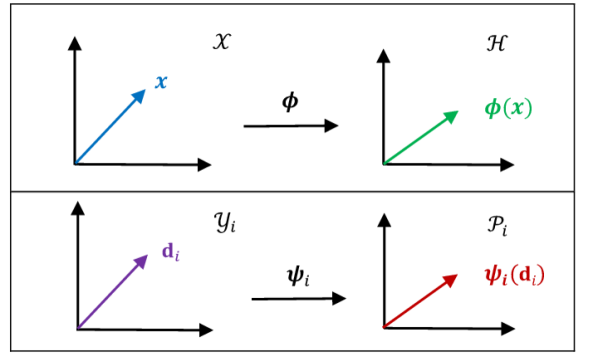
Figure 1: (Top) mapping inputs $\bm{x}$ to the Hilbert space $\mathcal{H}$ in initial modeling, (Bottom) mapping each hyperparameter vector $\bm{d}_{i}$ to its corresponding Hilbert space $\mathcal{P}_{i}$.

The KRLS algorithm has quadratic computational cost $\mathcal{O}(m^{2})$, where $m$ denotes the number of samples of the input vector Engel . Let the number of samples in each dimension be denoted by $m_{k}(k=0,1,\dots,n)$ for an $n+1$ dimensional system, then the algorithm cost is $\mathcal{O}((m_{0}m_{1}\dots m_{n})^{2})$, which can become quickly intractable.

2.2 2D Deep Kernel Recursive Least-Squares

Assume that the intention is to model a function with a two-dimensional input, denoted by $\bm{x}$ and $\bm{d}_{1}$ and one-dimensional output, denoted by $\bm{y}$. The output of this function is a function of the inputs $\bm{x}$ and $\bm{d}_{1}$, $f(\bm{x},\bm{d}_{1})$, and the objective of the modeling is to find this function, this is depicted in Figure 2.

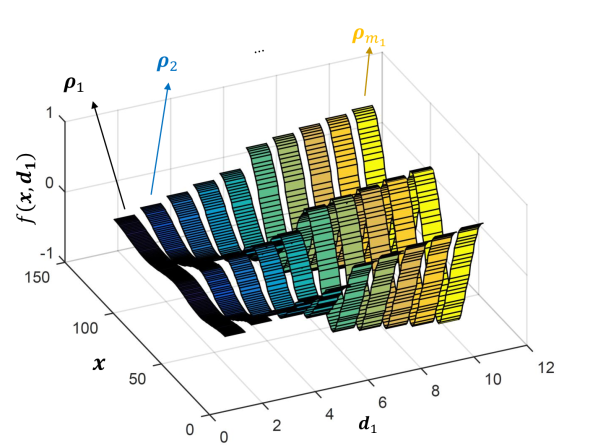
Figure 2: The two-dimensional function. Training is performed at each $\bm{d}_{1}$ sample and the corresponding weights ($\bm{\rho}_{1}$ to $\bm{\rho}_{m_{1}}$) are recorded.

In the first step, the modeling is performed on all the samples of $\bm{x}$ at the first sample of the $\bm{d}_{1}$ and the corresponding weight $\bm{\rho}_{1}$ is recorded. Then modeling is performed on all the samples of $\bm{x}$ at the next sample of $\bm{d}_{1}$. This process is continued until the last sample of $\bm{d}_{1}$, illustrated in Figure 3.

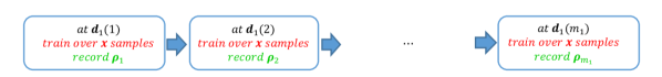
Figure 3: Training over all samples of $\bm{x}$ at each sample of $\bm{d}_{1}$ and recording the corresponding weights.

After recording $\bm{\rho}_{1}$ to $\bm{\rho}_{m_{1}}$, we put together these vectors and get a matrix $P$ as (2).

$$P=\begin{bmatrix}[\bm{\rho}_{1}]_{m_{0}\times 1}&[\bm{\rho}_{2}]_{m_{0}\times 1}&\dots&[\bm{\rho}_{m_{1}}]_{m_{0}\times 1}\\ \end{bmatrix}_{m_{0}\times m_{1}}.$$ (2)

The second step is to model each row of the matrix $P$ over $\bm{d}_{1}$ samples. To perform modeling, $m_{0}$ KRLS models are used as shown in Figure 4. Therefore, the dimension of the output is $m_{0}\times 1$. Accordingly, the corresponding weight $\xi$ recorded with dimension $m_{1}\times m_{0}$. This is the end of the training process.

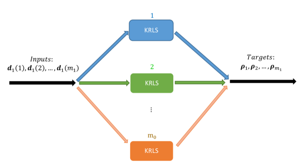
Figure 4: Modeling $\bm{\rho}_{1}$ to $\bm{\rho}_{m_{1}}$ by $m_{0}$ KRLS since dimension of the output is $m_{0}\times 1$.

The next step is to validate the model using a validation dataset. At the validation sample $j$ of $\bm{d}_{1}$ we can estimate $\Im_{j}$ by (3).

$$\Im_{j}=\begin{bmatrix}k_{H1}(\bm{d}_{1}(1),\bm{d}_{1val}(j))\\ k_{H1}(\bm{d}_{1}(2),\bm{d}_{1val}(j))\\ \vdots\\ k_{H1}(\bm{d}_{1}(m_{1}),\bm{d}_{1val}(j))\\ \end{bmatrix}_{m_{1}\times 1}$$ (3)

where $k_{H1}$ is the kernel function which is assumed to be Gaussian with the standard deviation $\sigma_{H1}$. Then, by using (4) and (5), we can estimate $\bm{\rho}_{j}$ and $P$, respectively.

$$[\bm{\hat{\rho}}_{j}]_{m_{0}\times 1}=[\xi]^{T}_{m_{0}\times m_{1}}[\Im_{j}]_{m_{1}\times 1}.$$ (4)

$$\hat{P}=\begin{bmatrix}[\bm{\hat{\rho}}_{1}]_{m_{0}\times 1}&[\bm{\hat{\rho}}_{2}]_{m_{0}\times 1}&\dots&[\bm{\hat{\rho}}_{m_{1}}]_{m_{0}\times 1}\\ \end{bmatrix}_{m_{0}\times m_{1val}}.$$ (5)

Then, at the validation sample $s$ of $\bm{x}$, we can calculate $\wp_{s}$ by using (6).

$$\wp_{s}=\begin{bmatrix}k_{I}(\bm{x}(1),\bm{x}_{val}(s))\\ k_{I}(\bm{x}(2),\bm{x}_{val}(s))\\ \vdots\\ k_{I}(\bm{x}(m_{0}),\bm{x}_{val}(s))\\ \end{bmatrix}_{m_{0}\times 1}$$ (6)

where $k_{I}$ is the kernel function which is assumed to be Gaussian with the standard deviation $\sigma_{I}$. In consequence, we can estimate the function $f(\bm{x},\bm{d}_{1})$ at any validation sample by (7).

$$f(s,j)=[{\bm{\hat{\rho}}_{j}}]^{T}_{1\times m_{0}}[\wp_{s}]_{m_{0}\times 1}.$$ (7)

The experimental results of this algorithm is presented in the subsections 3.1 and 3.3.

2.3 3D Deep Kernel Recursive Least-Squares

Consider a function with a three-dimensional input, denoted by $\bm{x}$, $\bm{d}_{1}$, and $\bm{d}_{2}$ and one-dimensional output, denoted by $\bm{y}$. The output is a function of the inputs $\bm{x}$, $\bm{d}_{1}$, and $\bm{d}_{2}$, and the aim of modeling is to find the function $f(\bm{x},\bm{d}_{1},\bm{d}_{2})$.

To execute modeling, at the first sample of $\bm{d}_{1}$ the modeling is performed on all samples of $\bm{x}$ and the corresponding weight $\bm{\vartheta}_{1,1}$ is recorded, with dimension $m_{0}\times 1$. Then modeling is performed on all samples of $\bm{x}$ at the next sample of $\bm{d}_{1}$ and the corresponding weight $\bm{\vartheta}_{2,1}$ is recorded. This process is continued until the last sample of $\bm{d}_{1}$ and recording the weight $\bm{\vartheta}_{m_{1},1}$. Next, this process is repeated for all samples of $\bm{d}_{2}$, illustrated in Figure 5, and the corresponding weights are recorded.

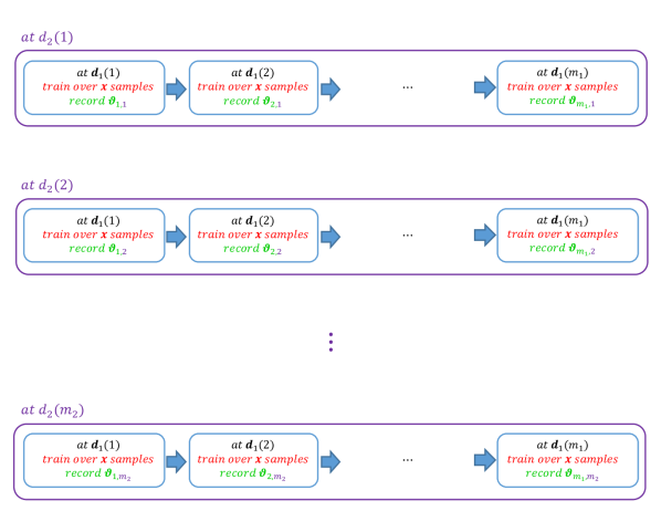
Figure 5: Training over all samples of $\bm{x}$ at each sample of $\bm{d}_{1}$ and at each sample of $\bm{d}_{2}$.

After recording $\bm{\vartheta}_{1,1}$ to $\bm{\vartheta}_{m_{1},m_{2}}$, we put together these weight vectors and we made a cell $\Theta$ according to (8). Consider that all of the elements of this cell are the weight vectors with dimension $m_{0}\times 1$.

$$\Theta=\begin{Bmatrix}[\bm{\vartheta}_{1,1}]&[\bm{\vartheta}_{1,2}]&\dots&[\bm{\vartheta}_{1,m_{2}}]\\ [\bm{\vartheta}_{2,1}]&[\bm{\vartheta}_{2,2}]&\dots&[\bm{\vartheta}_{2,m_{2}}]\\ \vdots&\vdots&\ddots&\vdots\\ [\bm{\vartheta}_{m_{1},1}]&[\bm{\vartheta}_{m_{1},2}]&\dots&[\bm{\vartheta}_{m_{1},m_{2}}]\\ \end{Bmatrix}_{m_{1}\times m_{2}}.$$ (8)

The second step is to model $\Theta$. Each column of $\Theta$ is correlated to one $\bm{d}_{2}$ sample and the desire is to model each of the columns one by one. Modeling each column of $\Theta$ is illustrated in Figure 6, which is done by $m_{0}$ KRLS since the dimension of each target vector is $m_{0}\times 1$.

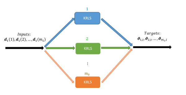
Figure 6: Modeling column $i$ of $\Theta$ by $m_{0}$ KRLS models.

After performing the modeling at each sample of $\bm{d}_{2}$, the corresponding weight $\beta_{1}$ to $\beta_{m_{2}}$ are recorded, the dimension of each weight is $m_{1}\times m_{0}$. This process is shown in Figure 7.

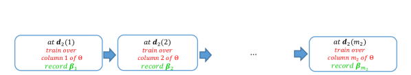
Figure 7: Training over column $i$ of $\Theta$ at each sample of $\bm{d}_{2}$ and recording the corresponding weights for $i=1,2,\dots,m_{2}$.

After recording $\beta_{1}$ to $\beta_{m_{2}}$, we put together these vectors and we made a cell as shown in (9).

$$\Omega=\{[\beta_{1}]_{m_{1}\times m_{0}},[\beta_{2}]_{m_{1}\times m_{0}},\dots,[\beta_{m_{2}}]_{m_{1}\times m_{0}}\}_{1\times m_{2}}.$$ (9)

The third step is to model $\Omega$. Each element of $\Omega$ ($\beta_{i}(i=1,2,\dots,m_{2})$) is a $m_{1}\times m_{0}$ matrix. As we need outputs to be in a vector format in KRLS modeling, we defined $\tilde{\beta}_{i}$ for $i=1,2,\dots,m_{2}$ and $\tilde{\Omega}$ as presented in (10) and (11) respectively.

$$\tilde{\beta}_{i}=\begin{bmatrix}\beta_{i}(:,1)\\ \beta_{i}(:,2)\\ \vdots\\ \beta_{i}(:,m_{0})\\ \end{bmatrix}_{m_{1}m_{0}\times 1}$$ (10)

where $(:,i)$ for $i=1,2,\dots,m_{2}$ denotes the column $i$th of a matrix.

$$\tilde{\Omega}=[\tilde{\beta}_{1},\tilde{\beta}_{2},\dots,\tilde{\beta}_{m_{2}}]_{m_{1}m_{0}\times m_{2}}.$$ (11)

Consider that each column of $\tilde{\Omega}$ is corresponded to one $\bm{d}_{2}$ sample and the intension is to model them one by one. Modeling of each column of $\tilde{\Omega}$ is illustrated in Figure 8.

Figure 8: Modeling $\bm{\tilde{\beta}}_{1}$ to $\bm{\tilde{\beta}}_{m_{2}}$ by $m_{1}m_{0}$ KRLS since dimension of the output is $m_{1}m_{0}\times 1$.

After performing the modeling, the corresponding weight $\gamma$ is recorded. The dimension of $\gamma$ is $m_{2}\times m_{1}m_{0}$. At this step modeling is finalized.
To validate the model, at the validation sample $i$ of $\bm{d}_{2}$ we can calculate $\eta_{i}$ by (12).

$$\eta_{i}=\begin{bmatrix}k_{H2}(\bm{d}_{2}(1),\bm{d}_{2val}(i))\\ k_{H2}(\bm{d}_{2}(2),\bm{d}_{2val}(i))\\ \vdots\\ k_{H2}(\bm{d}_{2}(m_{2}),\bm{d}_{2val}(i))\\ \end{bmatrix}_{m_{2}\times 1},$$ (12)

where $k_{H2}$ is the kernel function, which is assumed to be Gaussian with the standard deviation $\sigma_{H2}$. Then we estimate the weight $\tilde{\beta}_{i}$ by using (13).

$$[\hat{\tilde{\beta}}_{i}]_{m_{1}m_{0}\times 1}=[\gamma]^{T}_{m_{1}m_{0}\times m_{2}}[\eta_{i}]_{m_{2}\times 1}.$$ (13)

by reshaping $\hat{\tilde{\beta}}_{i}$ according to (10), we can find estimation of $\beta_{i}$, denoted by $\hat{\beta}_{i}$. Thus, we can find estimation of $\Omega$ by (14).

$$\begin{split}\hat{\Omega}=\{[\hat{\beta_{1}}]_{m_{1}\times m_{0}},[\hat{\beta_{2}}]_{m_{1}\times m_{0}},\dots,\\ [\hat{\beta}_{m_{1}}]_{m_{1}\times m_{0}}\}_{1\times m_{2val}}.\end{split}$$ (14)

Next, at the validation sample $j$ of $\bm{d}_{1}$ we can calculate $\tau_{j}$ by (15).

$$\tau_{j}=\begin{bmatrix}k_{H1}(\bm{d}_{1}(1),\bm{d}_{1val}(j))\\ k_{H1}(\bm{d}_{1}(2),\bm{d}_{1val}(j))\\ \vdots\\ k_{H1}(\bm{d}_{1}(m_{1}),\bm{d}_{1val}(j))\\ \end{bmatrix}_{m_{1}\times 1},$$ (15)

where $k_{H1}$ is the kernel function, which is assumed to be Gaussian with the standard deviation $\sigma_{H1}$. Then, we estimate the weight $\bm{\vartheta}_{i,j}$ by using (16) and consequently, we can find $\hat{\Theta}$ by (17).

$$[\bm{\hat{\vartheta}}_{i,j}]_{m_{0}\times 1}=[\hat{\beta_{i}}]^{T}_{m_{0}\times m_{1}}[\tau_{j}]_{m_{1}\times 1}.$$ (16)

$$\hat{\Theta}=\begin{Bmatrix}[\bm{\hat{\vartheta}}_{1,1}]&[\bm{\hat{\vartheta}}_{1,2}]&\dots&[\bm{\hat{\vartheta}}_{1,m_{2}}]\\ [\bm{\hat{\vartheta}}_{2,1}]&[\bm{\hat{\vartheta}}_{2,2}]&\dots&[\bm{\hat{\vartheta}}_{2,m_{2}}]\\ \vdots&\vdots&\ddots&\vdots\\ [\bm{\hat{\vartheta}}_{m_{1},1}]&[\bm{\hat{\vartheta}}_{m_{1},2}]&\dots&[\bm{\hat{\vartheta}}_{m_{1},m_{2}}]\\ \end{Bmatrix},$$ (17)

the dimension of $\hat{\Theta}$ is $m_{1val}\times m_{2val}$. Then, at the validation sample $s$ of $\bm{x}$ we can calculate $\iota_{s}$ by (18).

$$\iota_{s}=\begin{bmatrix}k_{I}(\bm{x}(1),\bm{x}_{val}(s))\\ k_{I}(\bm{x}(2),\bm{x}_{val}(s))\\ \vdots\\ k_{I}(\bm{x}(m_{0}),\bm{x}_{val}(s))\\ \end{bmatrix}_{m_{0}\times 1},$$ (18)

where $k_{I}$ is the kernel function, which is assumed to be Gaussian with the standard deviation $\sigma_{I}$. Then we estimate the weight $f(\bm{x},\bm{d}_{1},\bm{d}_{2})$ at any validation sample by using (19).

$$f(s,j,i)=[\bm{\hat{\vartheta}}_{i,j}]^{T}_{1\times m_{0}}[\iota_{s}]_{m_{0}\times 1}.$$ (19)

The implementation of this algorithm is in the subsection 3.2.

2.4 General Deep Kernel Recursive Least-Squares

In this part, we expand the presented idea for modeling higher dimensional datasets. The objective of the modeling is to find the function $f(\bm{x},\bm{d}_{1},\bm{d}_{2},\dots,\bm{d}_{n})$ in which inputs, denoted by $\bm{x}$, $\bm{d}_{1}$, $\bm{d}_{2}$ to $\bm{d}_{n}$.

Figure 9 illustrates the structure of the D-KRLS method in a general form. Consider a function with $n+1$ dimensional input, represented by $\bm{x},\bm{d}_{1},\bm{d}_{2},\dots,\bm{d}_{n}$, and with $m_{k}(k=0,1,\dots,n)$ samples in each dimension. The key idea is to perform training in multiple hierarchical steps. The algorithm consists of two major steps. The first step is called Initial Modeling in which modeling is performed over the first dimension ($\bm{x}$) and the corresponding weights are recorded at any sample of $\bm{d}_{1}$ to $\bm{d}_{n}$.

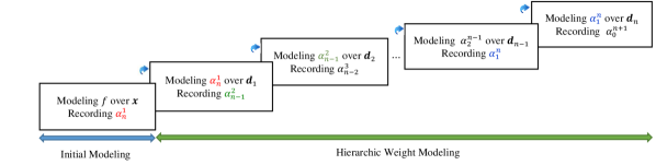
Figure 9: The structure of the D-KRLS method.

First $f$ is trained by KRLS and the corresponding weight vector $\bm{\alpha}_{0}^{1}$ is found, Figure 10 (Left). This training is performed $m_{0}\times m_{1}\times\dots\times m_{n}$ times to achieve complete model of $f$ at any sample of $\bm{d}_{1}$ to $\bm{d}_{n}$ by solving the optimization in (20) where $\bm{K}^{1}$ is the Gram matrix associated to the dimension $\bm{x}$ and where $\bm{y}_{k}$ is the desired target vector for $k=1,2,\dots,n+1$. Corresponding to Algorithm 1 ($i=0$), the superscript of the weight ($\alpha$) represents step and the subscript is the number of associated dimension that the corresponding weight is the result of training on those dimensions (i.e. number $0$ is used for the cases when the weight is not trained over any dimension).

$$\ell^{\prime}({\alpha}_{k-1}^{1})=\min_{{\alpha}_{k-1}^{1}}\|{K}^{1}{\alpha}_{k-1}^{1}-\bm{y}_{k}\|^{2},$$ (20)

The cost of Initial Modeling is $\mathcal{O}(m_{n}m_{n-1}\dots m_{1}(m_{0})^{2})$ .

Algorithm 1 D-KRLS Algorithm

  for $i=0$ to $n$ do

     for $k=1$ to $n+1-i$ do

        if $i=0$ then

           Initial Modeling

           $\min_{{\alpha}_{k-1}^{1}}\|{K}^{1}{\alpha}_{k-1}^{1}-\bm{y}_{k}\|^{2}$

        else if $i>0$ then

           Hierarchic Weight Modeling

           $\min_{{\alpha}_{k-1}^{i+1}}\|{K}^{i+1}{\alpha}_{k-1}^{i+1}-{\alpha}_{k}^{i}\|^{2}$

        end if

     end for

     Record: $\alpha_{n-i}^{i+1}$

  end for

 

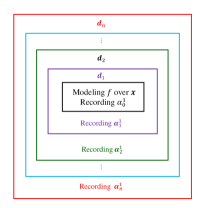
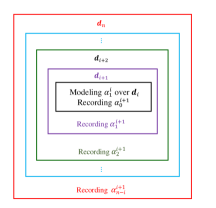
Figure 10: (Left) Initial Modeling; (Right) Hierarchic Weight Modeling.

The second step is called Hierarchic Weight Modeling as shown in Figure 10 (Right). In this step, first the weight $\bm{\alpha}_{1}^{i}$, is modeled over $\bm{d}_{i}$ for $i=1,2,\dots,n$. Assume $\bm{d}_{i}\in\mathcal{Y}_{i}$, for some space $\mathcal{Y}_{i}$. Therefore, there exist another Hilbert Space $\mathcal{P}_{i}$, and a mapping $\bm{\psi}_{i}:\mathcal{Y}_{i}\to\mathcal{P}_{i}$ such that $k(\bm{d}_{i},\bm{d}_{i}^{\prime})=\langle\bm{\psi}_{i}(\bm{d}_{i}),\bm{\psi}_{i}(\bm{d}_{i}^{\prime})\rangle_{\mathcal{P}_{i}}$, as shown in Figure 1 (Bottom). The training is performed by minimizing the loss function (21):

$$\ell^{\prime\prime}({\alpha}_{k-1}^{i+1})=\min_{{\alpha}_{k-1}^{i+1}}\|{K}^{i+1}{\alpha}_{k-1}^{i+1}-{\alpha}_{k}^{i}\|^{2},$$ (21)

where $k=1,2,\dots,(n+1-i)$ and $i=1,2,\dots,n$. It should be mentioned that the desired learning target in this step is the recorded weight from the previous step, namely $\bm{\alpha}_{k}^{i}$, which is correspond to the Algorithm 1 ($i>0$).

In summary, to model $f(\bm{x},\bm{d}_{1},\bm{d}_{2},\dots,\bm{d}_{n})$ it is required to train the corresponding weight $\alpha^{1}_{n}$. To model $\alpha^{1}_{n}$, it is required to train the corresponding weight $\alpha^{2}_{n-1}$ and to model $\alpha^{2}_{n-1}$ it is required to train the corresponding weight $\alpha^{3}_{n-2}$. This process continues until $\alpha^{n}_{1}$ is modeled, illustrated in Figure 9. The presented method uses a recursive formula and it has to be batch over the first $n$ dimensions, for a $n+1$ dimensional dataset.

2.5 Computational Efficiency of the D-KRLS Method

Although the approach in the above subsection seems complicated at first glance, it is in fact significantly more efficient compared to the KRLS method. The main reason is that the D-KRLS algorithm divides the training procedure into multiple steps, shown in Figure 9, and utilizes smaller sized kernel matrices instead of using one large sized kernel matrix. The total computational cost of the D-KRLS algorithm for a $n+1$ dimensional dataset is $\mathcal{O}(m_{n}m_{n-1}\dots m_{1}(m_{0})^{2}+m_{n}m_{n-1}\dots m_{2}(m_{1})^{2}+m_{n}m_{n-1}\dots m_{3}(m_{2})^{2}+\dots+m_{n}(m_{n-1})^{2}+(m_{n})^{2})$, which is significantly less than the KRLS method cost, $\mathcal{O}((m_{0}m_{1}\dots m_{n})^{2})$:

Proposition 1

Let $\bar{A}=m_{n}m_{n-1}\dots m_{1}(m_{0})^{2}+m_{n}m_{n-1}\dots m_{2}(m_{1})^{2}+\dots+m_{n}(m_{n-1})^{2}+(m_{n})^{2}$ denotes the computational cost of D-KRLS and $\bar{B}=(m_{0}m_{1}\dots m_{n})^{2}$ denotes the cost for KRLS. If the number of samples $m_{i}\geq 2,i\in(1,2,\dots,n)$ and $m_{0}=m_{1}=\dots=m_{n}$, then $\bar{A}<\bar{B}$.
The proof is presented in Appendix A.

Although Proposition 1 is restricted to $m_{0}=m_{1}=\dots=m_{n}$, the limit of the D-KRLS cost ($\bar{A}$) as $m_{i}$ (for $i=1,2,\dots,n$) approaches infinity, is less than the KRLS cost:

$$\begin{split}\lim_{m_{i(i=0,\dots,n)}\to\infty}\mathcal{O}(\bar{A})=\mathcal{O}(m_{n}m_{n-1}\dots m_{1}(m_{0})^{2})\\ <<\mathcal{O}((m_{0}m_{1}\dots m_{n})^{2}).\end{split}$$ (22)

3 Numerical Experiments

The D-KRLS method is exemplified on two synthetic and a real world datasets in subsections 3.1 to 3.3. Then, a discussion is presented regarding cross-correlation between space and time in subsection 3.4. Finally, in subsection 3.5 performance of the D-KRLS method is compared to the literature. It should be noted that all algorithms were implemented on an $Intel(R)Core(TM)i7-4700MQCPU@2.40GHz$ with $8GB$ of $RAM$ and the Gaussian kernel, $k(\bm{z},\bm{z}^{\prime})=exp(-(\bm{z}-\bm{z}^{\prime})^{T}(\bm{z}-\bm{z}^{\prime})/(2\sigma^{2}))$ is used in running all the algorithms herein.

3.1 Synthetic 2D Data Modeling

Exemplification of the D-KRLS method on a synthetic two-dimensional spatiotemporal function is presented in this subsection. The two-dimensional nonlinear function $\varUpsilon(\bm{x},\bm{d})$ is given by:

$$\varUpsilon(\bm{x},\bm{d})=\sin(\bm{x})cos(\frac{\bm{d}}{2}),$$ (23)

where $\bm{x}$ and $\bm{d}$ are arranged to be $145$ and $150$ evenly divided numbers ranging between $[0.1,4\pi]$ and $[0.1,8\pi]$ respectively, while the trigonometric functions are in radians. Consequently, by having $145$ and $150$ data points in each of the two directions, the total number of data points is $21750$. To train and validate, this dataset is divided randomly with $80\%$ of the data used for training and $20\%$ for validation in each dimension. For training, there are $116$ points in the $\bm{x}$ direction and $120$ points in the $\bm{d}$ direction and in total $13,920$ data points.

In the first step of the method, Initial Modeling is performed, using Algorithm 1 ($i=0$). The kernel matrix size equals $116\times 116$ as there are $116$ points in $\bm{x}$ direction and no sparsification is used to demonstrate maximum D-KRLS cost. The variance of the Gaussian kernel is found empirically to be $\sigma_{I}=1$. The corresponding weight $\bm{\alpha}_{0}^{1}$ of this matrix is a vector $116\times 1$. Initial Modeling took $2.80$ seconds for all $120$ data samples of $\bm{d}$. Then modeling of $\bm{\alpha}_{1}^{1}$ is done by Algorithm 1 ($i=1$). The kernel matrix size is equal to $120\times 120$ as there are $120$ points in $\bm{d}$ direction. The variance of the Gaussian kernel is found empirically to be $\sigma_{H1}=0.3$. The Weight Modeling took $0.13$ seconds. The cost of Initial Modeling is more than Hierarchic Weight Modeling, as the Initial Modeling training is done on all samples of $\bm{x}$ at all samples of $\bm{d}$. The total computational time for both steps to train D-KRLS is $2.93$ seconds. The corresponding error for validation is presented in Figure 11. For some data samples of $\bm{d}$ the error is bigger than the rest, as the same variance of the Gaussian kernel in Initial Modeling ($\sigma_{I}$) is used for all data samples over $\bm{d}$. Nevertheless, the maximum magnitude of recorded error is found to be $0.0134$, which indicates high validation accuracy.

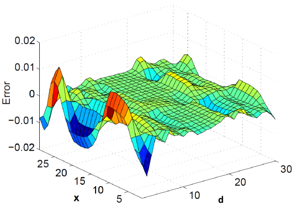
Figure 11: Validation error in modeling of the 2D synthetic dataset.

3.2 Synthetic 3D Data Modeling

To demonstrate the capability of the D-KRLS algorithm in modeling higher dimensional datasets, the presented algorithm is implemented on a synthetic three-dimensional function in this subsection. A three-dimensional function $\Xi(\bm{x},\bm{d}_{1},\bm{d}_{2})$ is defined as follows:

$$\Xi(\bm{x},\bm{d}_{1},\bm{d}_{2})=\cos(\bm{x})sin(\frac{\bm{d}_{1}}{2})sin(\frac{\bm{d}_{2}}{3}),$$ (24)

in which $\bm{x}$, $\bm{d}_{1}$, and $\bm{d}_{2}$ are arranged to be $145$, $150$, and $100$ evenly distributed numbers ranging between $[0.1,4\pi]$, $[0.1,8\pi]$, and $[0.1,12\pi]$ respectively, while the trigonometric functions are in radians. Consequently, the total number of the data points is equal to $2,175,000$, ($145\times 150\times 100$). To train and validate, this dataset is divided randomly with $80\%$ for training and $20\%$ for validation over each dimension. Therefore, there are $1,113,600$ data points for training ($116\times 120\times 80$) and $17,400$ points ($29\times 30\times 20$) for validation.

In the first step, Initial Modeling is performed, using Algorithm 1 ($i=0$). The kernel matrix is equal to $116\times 116$ as there are $116$ points in $\bm{x}$ direction. The variance of the Gaussian kernel in Initial Modeling is found empirically to be $\sigma_{I}=1$. The corresponding weight $\bm{\alpha}_{0}^{1}$ is a vector $116\times 1$. Initial Modeling took $900.8598$ seconds as the system is trained for all the samples of $\bm{d}_{1}$ and $\bm{d}_{2}$. Then modeling of $\bm{\alpha}_{2}^{1}$ is done by Algorithm 1 ($i=1$). The corresponding kernel matrix is equal to $120\times 120$ as there are $120$ points in $\bm{d}_{1}$ direction. It should be noted that the training of $\bm{\alpha}_{1}^{1}$ is a vector valued kernel model, as $\bm{\alpha}_{0}^{1}$ is a vector $116\times 1$ . Consequently, its corresponding weight $\bm{\alpha}_{0}^{2}$ is a matrix $120\times 116$ and it is formed here as a $13920\times 1$ vector. The variance of the Gaussian kernel is found empirically to be $\sigma_{H1}=0.3$. This process took $8.6569$ seconds as the system is trained for all the samples of $\bm{d}_{2}$. Then to have the model of $\bm{\alpha}_{2}^{1}$, it is required to model $\bm{\alpha}_{1}^{2}$ using Algorithm 1 ($i=2$). The corresponding kernel matrix is equal to $80\times 80$ as there are $80$ points in $\bm{d}_{2}$ direction and, using $\sigma_{H2}=1$ as the variance of the Gaussian kernel. This process took $0.7193$ seconds. The cost of training decreases for each step since there is one dimension less in each step compared to its previous step. The total computational time to train the D-KRLS method is $910.2360$ seconds. The corresponding maximum magnitude of the recorded error is found to be $0.0171$, which demonstrates high capability of D-KRLS in modeling of this dataset.

3.3 Temperature Modeling on Intel Lab Dataset

In this subsection, the presented algorithm is exemplified on a realistic two-dimensional spatiotemporal environment Intel in which $54$ sensors were arranged in Intel lab and the temperature is recorded. It is assumed herein that the sensor indices represent the location of the sensors over space, $\bm{x}$, and time, $\bm{d}$. The time, $\bm{d}$, is arranged from $301$ seconds to $400$ seconds (with $1$ second interval) and $52$ sensors are used (the sensors number $5$ and $15$ are not used to reduce outliers). Consequently, by having $100$ and $52$ data points in each direction, the total number of the data points equals $5200$. To reduce the outliers, the dataset is filtered by a 2D Gaussian filter with variance $5$ and size $6\times 6$. To train and validate, this dataset is divided over time randomly with $80\%$ for training and $20\%$ for validation. Totally, there are $4160$ data points for training, and there are $1040$ points for validation.

Therefore the total computational time to train the D-KRLS is $1.11$ seconds. The maximum magnitude of recorded error is found to be $3.11$, as the maximum values of the dataset is $25^{\circ}$C, the normalized error is $0.1244$.

3.4 Space-Time Cross-Correlation

This subsection emphasize on the importance of cross-correlations between dimensions. In the presented algorithm, all of the possible correlations between data points from different dimensions (i.g. space and time) are taken into account and no assumed predefined function is used in modeling of these correlations. In contrast, cross-correlations between space and time have been modeled in the literature by providing different space-time covariance functions crossfunction , such as:

$$\mathcal{C}(u,h)=\frac{1}{(a^{\prime 2}u^{2}+1)^{(\frac{1}{2})}}exp(-\frac{b^{\prime 2}h^{2}}{a^{\prime 2}u^{2}+1}),$$ (25)

in which $a^{\prime}$ and $b^{\prime}$ are scaling parameters of time and space respectively. We considered $\mathcal{C}$ as the input to KRLS, called the NONSTILL-KRLS method herein, inspired from NONSTILL-GP Garg2012 . In general, appropriate predefined function should result the same level of validation error compared to the KRLS method.

The results in this subsection are found by running the algorithms with $a^{\prime}=b^{\prime}=1$ on the dataset which is assumed to be a two-dimensional function, denoted in (23), where $\bm{x}$ and $\bm{d}$ are arranged to be $48$ and $50$ evenly distributed numbers ranging between $[0.1,0.4244]$ and $[0.1,0.8488]$ respectively, while the trigonometric functions are in radians. To train and validate, this dataset is divided randomly with $80\%$ of the data used for training and $20\%$ for validation in each dimension. For training, there are $37$ points in the $\bm{x}$ direction and $38$ points in the $\bm{d}$ direction and in total $1406$ data points. The reason for using a smaller sized dataset to compare to 2D synthetic dataset, described in subsection 3.1, is that KRLS and NONSTILL-KRLS add all data samples to their dictionary and consequently become extremely expensive and unable to model this large dataset. Hence, we used a smaller dataset in this subsection.

As tabulated in TABLE 1, NONSTILL-KRLS does not provide an appropriate level of accuracy because of its constraint to define a function in advance. Finding appropriate covariance functions and parameters of such functions is the main challenge. Also, computational time of NONSTILL-KRLS is very high and close to KRLS. On the other hand, the D-KRLS method (similar to KRLS) does not have any predefined model for correlations between space and time and, hence can achieve high level of accuracy.

Table 1: Comparison between D-KRLS, KRLS and NONSTILL-KRLS, in term of computational time in training and corresponding average and maximum validation errors.

Methods	Training Time	Average Validation Error	Maximum Validation Error
D-KRLS	0.3940 $s$	0.0029	0.0519
KRLS	22.6461 $s$	0.0035	0.0418
NONSTILL-KRLS	22.6675 $s$	0.0728	1.5323

3.5 Summary of Comparison with Existing Methods

In this section, the D-KRLS is compared with leading kernel-based modeling methods in the literature. Table 2 presents the comparison in terms of computational training time and maximum validation error of the presented algorithm with the studied kernel adaptive filtering algorithms in comparative : QKLMS QKLMS , FB-KRLS Fixed , S-KRLS Engel , SW-KRLS Sliding , and NORMA NORMA (the codes used here can be found in vanvaerenberghthesis ).

As detailed in TABLE 2, the D-KRLS method resulted in less computational time and also achieved lower maximum validation error compared to the other methods in the literature. For example, it is about five times faster and more accurate than S-KRLS in modeling the Intel Lab dataset. The hyperparameters that are used in running the algorithms are tabulated in TABLE 3 in Appendix B. Since the D-KRLS method results in an improvement in both computational time and accuracy, choosing different hyperparameter sets for the other algorithms, as a trade-off between accuracy and efficiency, does not change the general conclusion of this comparison. The results demonstrates that the D-KRLS method is much more efficient than the other methods, particularly for higher dimensional datasets. For the three-dimensional dataset, the majority of the methods fail and cannot provide a reasonably small validation error. However, D-KRLS models this dataset with high accuracy and less cost compared to all the other methods. Although, it is possible to perform modeling for higher dimensional datasets using D-KRLS, the comparison in TABLE 2 is limited to three-dimensional as the other methods in the literature fails in modeling of datasets above three-dimensional.

Table 2: Comparison between D-KRLS and other methods in the literature, in terms of computational time in training the datasets and corresponding maximum validation errors.

Methods	2D dataset	3D dataset	Intel Lab dataset
	13,920 Samples	1,113,600 Samples	4,160 Samples
	(Time — Error)	(Time — Error)	(Time — Error)
D-KRLS	2.93 $s$ — 0.0134	910.23 $s$ — 0.0171	1.11 $s$ — 0.1244
QKLMS	39.39 $s$ — 0.8401	68168.58 $s$ — 0.4469	1.54 $s$ — 0.6220
FB-KRLS	285.76 $s$ — 0.0572	12994.17 $s$ — 0.9232	39.88 $s$ — 0.2182
S-KRLS	108.66 $s$ — 0.0232	4608.40 $s$ — 0.8067	5.64 $s$ — 0.1582
NORMA	38.61 $s$ — 0.3502	2309.76 $s$ — 0.9949	1.49 $s$ — 0.3422
SW-KRLS	1097.26 $s$ — 0.9971	7696.30 $s$ — 0.9949	288.77 $s$ — 0.9895

4 Conclusion

We presented a kernel method for modeling evenly distributed multidimensional datasets. The proposed approach utilizes a new hierarchic fashion to model weights of each dimension over its adjacent dimension. The presented deep kernel algorithm was compared against a number of leading kernel least squares algorithms and was shown to outperform in both accuracy and computational cost. The method provides a different perspective that can lead to new techniques for scaling up kernel-based models for multidimensional datasets.

Appendix A Proof

Proof

The proof is done by induction.

Let $n=1$:
$m_{1}(m_{0})^{2}<(m_{0}m_{1})^{2}$ as $m_{0}=m_{1}=...=m_{n}=m$ and $m_{i}\geq 2$ for $i=1,2,...,n$. Therefore, $m^{3}<m^{4}$ and the proposition holds for $n=1$.
Assume for $n=k$ the Proposition holds:
$\bar{A}-\bar{B}<0$.
Let $n=k+1$: Therefore the statement $\bar{A}-\bar{B}<0$ can be written as:

$m_{k+1}m_{k}m_{k-1}...m_{1}(m_{0})^{2})+m_{k+1}m_{k}m_{k-1}...m_{2}(m_{1})^{2}+...+m_{k+1}(m_{k})^{2}+(m_{k+1})^{2}-(m_{0}m_{1}...m_{k}m_{k+1})^{2}<0$,
$\Rightarrow m_{k+1}\bar{A}+(m_{k+1})^{2}-\bar{B}(m_{k+1})^{2}<0$,
as $m_{0}=m_{1}=...=m_{n}=m$, therefore $m\bar{A}+m^{2}-\bar{B}m^{2}<0$,
$\Rightarrow\bar{A}m^{2}-\bar{A}m^{2}+m\bar{A}+m^{2}-\bar{B}m^{2}<0$,
$\Rightarrow m^{2}(\bar{A}-\bar{B})-\bar{A}m^{2}+m\bar{A}+m^{2}<0$,
as $\bar{A}-\bar{B}<0$, the first term is always negative and therefore it is sufficient to show that summation of the other terms is also negative.
$\Rightarrow-\bar{A}m^{2}+m\bar{A}+m^{2}<0$,
$\Rightarrow m(\bar{A}-m\bar{A})+m^{2}<0$,
$\Rightarrow m\bar{A}(1-m)+m^{2}<0$,
$\hat{A}=m\bar{A}$, $\Rightarrow\hat{A}(1-m)+m^{2}<0$,
$\Rightarrow\hat{A}(1-m)<-m^{2}$,
$\Rightarrow\frac{\hat{A}(-1+m)}{m^{2}}>1$,
$\Rightarrow(m^{k+1}+m^{k}+...+m^{2}+m^{1})(-1+m)>1$,
$\Rightarrow m^{k+2}-m>1$,
$\Rightarrow m(m^{k+1}-1)>1$,
$\Rightarrow(m^{k+1}-1)>\frac{1}{m}$,
As $m\geq 2$, the right hand side is always equal or less than 0.5 and the left hand side is always equal or greater than 1, therefore the statement holds for $n=k+1$.

Appendix B Hyperparameters

The hyperparameters used in running the algorithms are tabulated in Table 3.

Table 3: The hyperparameters used in the section III.

Methods	Synthetic 2D	Synthetic 3D	Intel Lab
D-KRLS
($\sigma_{I},\sigma_{H1},(\sigma_{H2})$)	1, 0.3	1, 0.3, (1)	1, 1.5
QKLMS
($\sigma$, $\mu$)	1, 0.15	0.5, 0.03	3.5, 0.15
($\epsilon$ )	$10^{-6}$	0.0005	$10^{-6}$
FB-KRLS
($\sigma$, $D$)	1, 800	0.5, 600	3.5, 500
($\lambda$, $\mu$)	0.1, 0	0.01, 0.03	0.01, 0.03
S-KRLS
($\sigma,\delta$)	1, 0.01	1, 0.99	3.5, 0.2
NORMA
($\sigma$, $D$)	1, 13920	1, $10^{+4}$	3.5, 4160
($\eta$, $\lambda$)	0.02, +$10^{-4}$	0.005, $10^{-7}$	0.04, $10^{-6}$
SW-KRLS
($\sigma$, $D$)	1, 1000	1, 300	3.5, 1000
($c$)	0.01	0.01	0.01

References

- (1) N. Tryfona, C. Jensen, GeoInformatica 3(3), 245 (1999). DOI 10.1023/A:1009801415799. URL http://dx.doi.org/10.1023/A%3A1009801415799
- (2) S. Vedula, S. Baker, T. Kanade, ACM Trans. Graph. 24(2), 240 (2005). DOI 10.1145/1061347.1061351
- (3) C.M. Bishop, Pattern Recognition and Machine Learning (Information Science and Statistics) (Springer-Verlag New York, Inc., Secaucus, NJ, USA, 2006)
- (4) S. Van Vaerenbergh, J. Via, I. Santamaria, in Acoustics, Speech and Signal Processing, 2006. ICASSP 2006 Proceedings. 2006 IEEE International Conference on, vol. 5 (2006), vol. 5. DOI 10.1109/ICASSP.2006.1661394
- (5) J. Kivinen, A. Smola, R. Williamson, Signal Processing, IEEE Transactions on 52(8), 2165 (2004). DOI 10.1109/TSP.2004.830991
- (6) S. Van Vaerenbergh, I. Santamaria, W. Liu, J. Principe, in Acoustics Speech and Signal Processing (ICASSP), 2010 IEEE International Conference on (2010), pp. 1882–1885. DOI 10.1109/ICASSP.2010.5495350
- (7) S. Van Vaerenbergh, M. Lazaro-Gredilla, I. Santamaria, Neural Networks and Learning Systems, IEEE Transactions on 23(8), 1313 (2012). DOI 10.1109/TNNLS.2012.2200500
- (8) B. Chen, S. Zhao, P. Zhu, J. Principe, Neural Networks and Learning Systems, IEEE Transactions on 23(1), 22 (2012). DOI 10.1109/TNNLS.2011.2178446
- (9) K. Li, J.C. Príncipe, IEEE Transactions on Signal Processing 65(24), 6520 (2017). DOI 10.1109/TSP.2017.2752695
- (10) S. Garcia-Vega, X.J. Zeng, J. Keane, Neurocomputing 339, 105 (2019). DOI 10.1016/j.neucom.2019.01.055
- (11) Y. Engel, S. Mannor, R. Meir, Signal Processing, IEEE Transactions on 52(8), 2275 (2004). DOI 10.1109/TSP.2004.830985
- (12) M. Han, S. Zhang, M. Xu, T. Qiu, N. Wang, IEEE Transactions on Cybernetics 49(4), 1160 (2019). DOI 10.1109/TCYB.2018.2789686
- (13) Y. Zheng, S. Wang, J. Feng, C.K. Tse, Digital Signal Processing 48, 130 (2016). DOI 10.1016/j.dsp.2015.09.015
- (14) H. Fan, Q. Song, Z. Xu, in IECON 2012 - 38th Annual Conference on IEEE Industrial Electronics Society (2012), pp. 1574–1579. DOI 10.1109/IECON.2012.6388534
- (15) W. Gao, J. Chen, IEEE Signal Processing Letters 24(7), 996 (2017). DOI 10.1109/LSP.2017.2702714
- (16) W. Gao, J. Chen, C. Richard, J. Huang, in 2015 IEEE 6th International Workshop on Computational Advances in Multi-Sensor Adaptive Processing (CAMSAP) (2015), pp. 217–220. DOI 10.1109/CAMSAP.2015.7383775
- (17) P. Bouboulis, S. Chouvardas, S. Theodoridis, IEEE Transactions on Signal Processing 66(7), 1920 (2018). DOI 10.1109/TSP.2017.2781640
- (18) C. Plagemann, K. Kersting, W. Burgard, in Machine learning and knowledge discovery in databases (Springer, 2008), pp. 204–219
- (19) S. Garg, A. Singh, F. Ramos, in Proceedings of the Twenty-Sixth AAAI Conference on Artificial Intelligence, July 22-26, 2012, Toronto, Ontario, Canada. (2012)
- (20) K. Mardia, C. Goodall, E. Redfern, F. Alonso, Test 7(2), 217 (1998). DOI 10.1007/BF02565111. URL http://dx.doi.org/10.1007/BF02565111
- (21) X.W. Chen, X. Lin, IEEE Access 2, 514 (2014). DOI 10.1109/ACCESS.2014.2325029
- (22) A. Damianou, N. Lawrence, in Proceedings of the Sixteenth International Workshop on Artificial Intelligence and Statistics (AISTATS-13), ed. by C. Carvalho, P. Ravikumar (JMLR W&CP 31, 2013), AISTATS ’13, pp. 207–215
- (23) V.N. Vapnik, Statistical Learning Theory (Wiley-Interscience, 1998)
- (24) P. Bodik, W. Hong, C. Guestrin, S. Madden, M. Paskin, R. Thibaux. Intel lab data, available on 2016-03-21. URL http://db.csail.mit.edu/labdata/labdata.html
- (25) N. Cressie, H.C. Huang, Journal of the American Statistical Association 94(448), pp. 1330 (1999)
- (26) S. Van Vaerenbergh, I. Santamaria, in Digital Signal Processing and Signal Processing Education Meeting (DSP/SPE), 2013 IEEE (2013), pp. 181–186. DOI 10.1109/DSP-SPE.2013.6642587
- (27) S. Van Vaerenbergh, Kernel methods for nonlinear identification, equalization and separation of signals. Ph.D. thesis, University of Cantabria (2010)