A Temporal Slow Growth Formulation for Direct Numerical Simulation of Compressible Wall–Bounded Flows

Abstract

A new slow growth formulation for DNS of wall-bounded turbulent flow is developed and demonstrated to enable extension of slow growth modeling concepts to complex boundary layer flows. As in previous slow growth approaches, the formulation assumes scale separation between the fast scales of turbulence and the slow evolution of statistics such as the mean flow. This separation enables the development of approaches where the fast scales of turbulence are directly simulated while the forcing provided by the slow evolution is modeled. The resulting model admits periodic boundary conditions in the streamwise direction, which avoids the need for extremely long domains and complex inflow conditions that typically accompany spatially developing simulations. Further, it enables the use of efficient Fourier numerics. Unlike previous approaches (Spalart, 1988; Guarini et al., 2000), the present approach is based on a temporally evolving boundary layer and is specifically tailored to give results for calibration and validation of RANS turbulence models. The use of a temporal homogenization simplifies the modeling, enabling straightforward extension to flows with complicating features, including cold and blowing walls. To generate data useful for calibration and validation of RANS models, special care is taken to ensure that the mean slow growth forcing is closed in terms of the mean and other quantities that appear in standard RANS models, ensuring that there is no confounding between typical RANS closures and additional closures required for the slow growth problem. The performance of the method is demonstrated on two problems: an essentially incompressible, zero-pressure-gradient boundary layer and a transonic boundary layer over a cooled wall with wall transpiration. The results show that the approach produces flows that are qualitatively similar to other slow growth methods as well as spatially developing simulations and that the new method can be a useful tool in investigating complex wall–bounded flows.

I Introduction

Direct numerical simulation (DNS) is a valuable tool for investigating turbulent boundary layers. DNS is of particular value to the formulation, calibration, and testing of engineering turbulence models, such as Reynolds Averaged Navier-Stokes (RANS) models, because the conditions in which the turbulence evolves are precisely defined, making it possible for model-based simulations to be performed under conditions that exactly match those in which the data is generated. Another important use of boundary layer DNS is the study of the structure and statistics of the turbulence. In this case, the ability to access three dimensional time-dependent turbulent velocity and scalar fields is of great value. Furthermore, experimental measurements in turbulent boundary layers are often difficult and limited, especially in the presence of complicating features such as transpiration, compressibility, and chemical reactions. In these situations, DNS can provide data that would not otherwise be available. In this work, we aim to develop DNS model problems that are 1) well-suited to generating data for turbulence model calibration and testing in boundary layers and 2) easily generalizable to complex situations to enable the study of complex boundary layers.

The DNS of spatially developing boundary layers, which most often occur in reality, presents challenges. The biggest issue is the very long evolution lengths that are required for the turbulence to equilibrate and eliminate artifacts of artificial inlet boundary conditions. This issue also arises in experiments, where a long distance is required for a boundary layer to relax to a canonical turbulent boundary layer downstream of a trip. However, in the case of DNS, this long evolution requires very large computational domains and, consequently, great computational costs Sillero et al. (2013). The importance of this issue was highlighted by Schlatter & Örlü (2010) who found that, even considering only well-resolved simulations, results for DNS of incompressible, low Reynolds number, turbulent boundary layers show disconcerting inconsistencies. They concluded that the discrepancies are due to difficulties associated with spatially developing simulations, including limited domain sizes and inflow boundary data.

The required streamwise domain size of a DNS of a spatially evolving boundary layer can be minimized with realistic inflow boundary conditions. Formulation of appropriate inflow conditions for spatially evolving simulations is a well-known problem. Often, an auxiliary simulation or a recycling/rescaling procedure is used. While such procedures have been the subject of ongoing research for over 20 years (Wu, 2017), they still introduce implementation complexities and modeling challenges. For instance, even in the best understood scenario, a canonical zero-pressure-gradient flat plate boundary layer, where the method of Lund et al. (1998) has been used successfully, recycling/rescaling procedures have the potential to introduce spurious periodicity (Nikitin, 2007) and other issues (Jewkes et al., 2011). In cases with additional complicating phenomena, such as wall transpiration or chemical reactions, the challenges associated with posing appropriate inflow conditions can only increase.

Motivated by the difficulties of simulating spatially evolving boundary layers, Spalart (1988) developed a “slow growth” approximation, in which the effects of the slow streamwise evolution are modeled while the turbulent fluctuations are directly simulated. Slow growth approaches rely on an assumed separation of scales between the fast evolution of the turbulent fluctuations and the slow evolution of mean characteristics of the boundary layer. Because of this separation, one can conduct a DNS of the fast evolution at a single, fixed point in the slow evolution, with slow evolution effects modeled. In a slow growth formulation, the fast scale turbulence becomes homogeneous in the streamwise direction. This allows the use of periodic boundary conditions in the streamwise direction, eliminating the need for turbulent inflow boundary conditions or an exceptionally long streamwise domain size. Further, homogeneity enables the use of Fourier spectral methods, which are the preferred numerical discretizations for DNS due to their efficiency and good resolution properties.

In the work presented here, a new slow growth DNS model is developed and applied. The approach is based on homogenization in time, rather than space, and an assumption of self-similarity in the slow evolution. It is constructed to support calibration and validation of RANS turbulence models for compressible boundary layers with transpiration and to be generalizable to boundary layers with complicating physical phenomena such as chemical reactions and favorable pressure gradients. Naturally, because of the approximations required to formulate a slow growth DNS, the resulting homogenized boundary layer will necessarily differ from a spatially developing layer. As will be shown in Section III, the temporal slow growth turbulent boundary layers obtained here resemble spatially evolving layers to a degree comparable to previous spatially homogenized boundary layers. Whether the remaining differences are important depends on the goals of the simulation. If the goal is to learn as much as possible about the features of a particular spatially evolving flow, then a spatially developing simulation is best. In this case, it is worth the time and effort required to overcome the challenges associated with inflow boundary conditions and long domain sizes noted previously.

However, if the goal is to learn more generally about features of wall–bounded turbulence—including, for example, the ability of RANS models to represent the effects of turbulence in such flows or how the turbulence is affected by complicating physical phenomena (e.g., chemistry)—it is not necessarily crucial to simulate a spatially developing boundary layer. Instead, there are two requirements. First, the fast turbulent scales must be governed by the Navier–Stokes equations with forcing provided by the slow evolution. Second, the modeled effect of the slow evolution must be sufficiently representative of the flow of interest. Thus, it is not necessary that the effects of the slow evolution be represented exactly, and in fact, one may be willing to tolerate differences in the name of simplicity if their effects can be understood. This realization enables the development of a slow growth modeling approach that is easily extensible to increasingly complex physical phenomena, allowing straightforward and computationally efficient investigations of the effects of these complicating phenomena on wall-bounded turbulence.

I.1 Previous Slow Growth Formulations

By modeling the forcing due to the slow evolution, slow growth homogenization formulations enable efficient simulation of turbulence that is representative of that in an evolving flow. The slow growth simulation concept was pioneered for incompressible turbulent boundary layers in a series of papers (Spalart & Leonard, 1985; Spalart, 1986) which culminated in simulation of an incompressible, zero-pressure-gradient turbulent boundary layer with Reynolds number up to $Re_{\theta}=1410$ (Spalart, 1988). The approach was later extended to compressible flows by Guarini et al. (2000) and used to simulate a $M_{\infty}=2.5$, $Re_{\theta}=1577$, adiabatic wall boundary layer. Both Spalart (1988) and Guarini et al. (2000) formulated slow growth models based on a coordinate transform combined with a multi-scale analysis. In these approaches, the coordinate transformation is designed to fit the boundary layer growth, with the goal that, for a section of small streamwise extent, the flow is approximately homogeneous in the transformed streamwise direction. Then, a multi-scale analysis is performed to split the streamwise variation into slow and fast components. The result of the analysis is a set of equations governing the fast component of the flow at a single point in the slow streamwise evolution. These equations are formally equivalent to the Navier–Stokes equations with the addition of source terms that quantify the effect of the slow evolution. Then, to enable a slow growth simulation, the source terms are modeled to close the system.

In the context of the current work, the existing slow growth formulations have two main drawbacks. First, as formulated by Guarini et al. (2000), many modeling assumptions are required in the compressible regime. For instance, the van Driest relationship is used to relate mean temperature and streamwise velocity, and it is assumed that the van Driest transformed velocity satisfies typical incompressible scaling laws. These assumptions do not necessarily hold for more general situations, and it is unclear how to extend the formulation to such cases.

The second difficulty is specific to using the data resulting from slow growth DNS for calibration and validation of RANS turbulence models. In doing so, one will naturally be required to solve the Reynolds–averaged slow growth equations, which are obtained by applying the Reynolds averaging procedure to the slow growth equations. The resulting equations govern the mean flow at a particular point in the slow evolution and contain all the usual unclosed terms—e.g., the Reynolds stress—as well as the Reynolds average of the slow growth sources, which represent the mean forcing provided by the slow evolution. Thus, to avoid confounding errors introduced by the standard RANS closures with those introduced by additional models required to close the mean slow growth sources, it is necessary for the mean slow growth source terms to be closed purely in terms of the mean flow and quantities that are already modeled as part of a standard RANS model. Neither the Spalart nor the Guarini formulations satisfy this requirement.

I.2 Overview

To overcome these limitations of existing slow growth DNS models, a new formulation is developed and presented in this work. The approach is based on homogenization of a temporally evolving boundary layer. Thus, the motivating flow is the classical temporal boundary layer, where an infinite plate is impulsively started at time $t=0$. In this situation, a boundary layer develops over the plate. This boundary layer is naturally homogeneous in the streamwise and spanwise directions, inhomogeneous in the wall–normal direction, and non–stationary since it grows in time. Thus, unlike the approaches of Spalart (1988) and Guarini et al. (2000), this formulation requires homogenization in time rather than space. This switch enables the development of more easily extensible models for the slow growth forcing terms. Section II gives details of this formulation, including constraints imposed by the RANS calibration and validation use case and the specific modeling assumptions invoked to develop a concrete model. Then, two sets of example results are reported in Section III. To show how the results of the present formulation differ from previous slow growth models, Section III.1 compares statistics from the present formulation for a $M_{\infty}=0.3$ turbulent boundary layer to those from a slow growth simulation due to Spalart (1988) and a spatially evolving simulation due to Schlatter & Örlü (2010). To demonstrate the applicability of the approach to more complex flows, Section III.2 shows statistics from a transonic turbulent boundary layer with a cold wall and wall transpiration. The cold wall and transpiration are seen to have dramatic effects on both the mean velocity profile and turbulence quantities near the wall. Section IV provides conclusions and directions for future work.

II Temporal Slow Growth Formulation

This section describes a temporal slow growth DNS model designed to yield data useful for calibration and validation of RANS models. In the development to follow, $\rho$ will denote the fluid density, $u_{i}$ the velocity vector in Cartesian tensor notation, and $E=e+u_{k}u_{k}/2$ the total energy per unit mass, including the internal energy ($e$) and the kinetic energy. Einstein summation convention will be used throughout. The spatial position vector is $x_{i}$, with the wall-normal coordinate also designated as $y$. Reynolds averaging will be denoted by an overbar, and the Reynolds fluctuations by a single prime. Thus, the Reynolds decomposition of the density is given by $\rho=\overline{\rho}+\rho^{\prime}$. The Favre, or density-weighted, average will be denoted by a tilde, and the Favre fluctuations by a double prime. So, the Favre decomposition of the velocity is given by $u_{i}=\tilde{u}_{i}+u^{\prime\prime}_{i}=\overline{\rho u}_{i}/\overline{\rho}+u^{\prime\prime}_{i}$.

II.1 Multi-scale Formulation and RANS

As described in Section I, a statistically stationary slow growth model is sought for a temporally evolving turbulent boundary layer developing over an impulsively started infinite flat plate. The evolution of such a boundary layer is described by the compressible Navier–Stokes equations, written here in a generic form that will facilitate the analysis to follow:

$$\frac{\partial\rho q}{\partial t}+\mathcal{N}_{\rho q}=0.$$ (1)

Here, $q$ represents one of the five conserved quantities per unit mass. That is, $q$ is either 1, one of the velocity components $u_{i}$ or the total energy per unit mass $E$, so that the volume density of the conserved quantities are $\rho$ for mass, $\rho u_{i}$ for momentum, and $\rho E$ for energy. The quantities $\rho$ and $q$ make up the so-called primitive variables. The symbol $\mathcal{N}_{\rho q}$ then represents all the remaining terms in the equation for $\rho q$ in the Navier-Stokes equations. For example, $\mathcal{N}_{\rho}=\partial\rho u_{i}/\partial x_{i}$.

The slow growth formulation developed here is based on the assumption that the boundary layer grows much more slowly than the evolution of the turbulence. This motivates the use of a multi-time-scale asymptotic formulation in terms of a fast time $t_{f}=t$ and a slow time $t_{s}=\epsilon t$, where $\epsilon\ll 1$. The turbulence fluctuations are presumed to evolve in fast time $t_{f}$, whereas mean quantities evolve only in slow time $t_{s}$. Introducing this two-time formulation into the Navier-Stokes equations yields

$$\frac{\partial\rho q}{\partial t_{f}}+\mathcal{N}_{\rho q}=-\epsilon\frac{\partial\rho q}{\partial t_{s}}.$$ (2)

The objective is to perform a DNS of the Navier-Stokes equations in fast time $t_{f}$ at some constant value of the slow time $t_{s}=t_{0}$. For an impulsively started plate, the boundary layer thickness is just a function of $t_{s}$, and so specifying $t_{s}=t_{0}$ is equivalent to defining the boundary layer thickness and therefore the Reynolds number of the DNS. The DNS will thus solve the equations

$$\frac{\partial\rho q}{\partial t_{f}}+\mathcal{N}_{\rho q}=\mathcal{S}_{\rho q}=\left.-\epsilon\frac{\partial\rho q}{\partial t_{s}}\right|_{t_{s}=t_{0}},$$ (3)

where $\mathcal{S}_{\rho q}$ is referred to as the slow growth source, which must be modeled. In addition to (3), it will be convenient to consider the primitive variable form of the slow growth Navier-Stokes equations

$$\frac{\partial\rho}{\partial t_{f}}+\mathcal{N}_{\rho}=\mathcal{S}_{\rho},$$ (4)

$$\frac{\partial q}{\partial t_{f}}+\mathcal{N}_{q}=\mathcal{S}_{q}.$$ (5)

where in the usual way

$$\mathcal{N}_{q}=\frac{1}{\rho}(\mathcal{N}_{\rho q}-q\mathcal{N}_{\rho}),$$ (6)

$$\mathcal{S}_{q}=\frac{1}{\rho}(\mathcal{S}_{\rho q}-q\mathcal{S}_{\rho}).$$ (7)

In formulating models for the slow growth source $\mathcal{S}_{\rho q}$, it will be important to consider how the source terms enter the RANS equations. If the sources in the RANS equations are closed with respect to the RANS state variables, then a RANS of the resulting slow growth system will not require any additional modeling assumptions besides those inherent to the RANS model. The RANS equations are obtained by averaging the Navier-Stokes equations. Because the temporally homogenized turbulent boundary layer will be statistically stationary, this procedure gives simply

$$\overline{\mathcal{N}_{\rho q}}=\overline{\mathcal{S}_{\rho q}}.$$ (8)

In addition, RANS models generally involve one or more auxiliary equations for turbulence quantities, such as the turbulent kinetic energy per unit mass $k=\widetilde{u^{\prime\prime}_{i}u^{\prime\prime}_{i}}/2$ and the turbulent energy dissipation rate per unit mass $\epsilon$, in the $k$-$\epsilon$ equation. Another common auxiliary equation in RANS models is the equation for the Reynolds stress tensor $R_{ij}=\overline{\rho u^{\prime\prime}_{i}u^{\prime\prime}_{j}}$. Because, $k=R_{ii}/2\overline{\rho}$, it will be sufficient to consider just the Reynolds stress equation, which reduces to

$$\underbrace{\overline{u_{i}^{\prime\prime}u_{j}^{\prime\prime}\mathcal{N}_{\rho}+\rho u_{i}^{\prime\prime}\mathcal{N}_{u_{j}}+\rho u_{j}^{\prime\prime}\mathcal{N}_{u_{i}}}}_{\overline{\mathcal{N}_{R_{ij}}}}=\underbrace{\overline{u_{i}^{\prime\prime}u_{j}^{\prime\prime}\mathcal{S}_{\rho}+\rho u_{i}^{\prime\prime}\mathcal{S}_{u_{j}}+\rho u_{j}^{\prime\prime}\mathcal{S}_{u_{i}}}}_{\overline{\mathcal{S}_{R_{ij}}}}.$$ (9)

To avoid RANS modeling of terms arising from the slow growth source terms, we will require that the right hand sides of (8-9) be closed in terms of the RANS state variables.

For simplicity, we do not require that the slow growth source term in the dissipation rate equation be closed. However, for constant density, constant viscosity flows, the formulation shown in Section II.3 does result in a dissipation equation slow growth source that is closed in terms of $\epsilon$ and $k$. This result does not hold for a general compressible flow. However, in non-hypersonic wall-bounded flows, the dissipation is dominated by the solenoidal component Huang et al. (1995); Guarini et al. (2000); Sinha & Candler (2003). We therefore expect that a closure model based on the incompressible result would adequately model the effect of the slow growth sources for many cases of interest.

II.2 RANS-Consistent Slow Growth Sources

As is shown in Appendix A, a straightforward formulation of the slow growth sources in terms of the conserved variables leads to sources in the RANS equations that are unclosed. Here it is shown that a formulation based on the primitive variable source terms can yield RANS source terms that are closed. Consider the following slow growth source term formulation:

$$\mathcal{S}_{\rho} =\rho f_{\rho},$$ (10)

$$\mathcal{S}_{q} =g_{q}+q^{\prime\prime}h_{q},$$ (11)

where the functions $f_{\rho}$, $g_{q}$, and $h_{q}$ depend only on $y$ and are expressed in terms of the statistical quantities that serve as state variables in the RANS models. When these forms are used to write the RANS slow growth sources in (8) using (7), the results are

$$\overline{\mathcal{S}_{\rho}}=\overline{\rho}f_{\rho},$$

$$\overline{\mathcal{S}_{\rho q}}=\overline{q\mathcal{S}_{\rho}}+\overline{\rho\mathcal{S}_{q}}=\overline{\rho q}f_{\rho}+\overline{\rho}g_{q}+\underbrace{\overline{\rho q^{\prime\prime}}}_{=0}h_{q}=\overline{\rho q}f_{\rho}+\overline{\rho}g_{q}.$$

Thus, the mean slow growth sources are closed purely in terms of the RANS variables $\overline{\rho}$, $\overline{\rho q}$, and the dependencies of $f_{\rho}$ and $g_{q}$. Similarly expanding the source in the Reynolds stress transport equations—i.e., the right hand side of (9)—yields

$$\overline{\mathcal{S}_{R_{ij}}} =\overline{u_{i}^{\prime\prime}u_{j}^{\prime\prime}\mathcal{S}_{\rho}}+\overline{\rho u_{i}^{\prime\prime}\mathcal{S}_{u_{j}}}+\overline{\rho u_{j}^{\prime\prime}\mathcal{S}_{u_{i}}}$$

$$=\overline{R_{ij}}f_{\rho}+\underbrace{\overline{\rho u_{i}^{\prime\prime}}g_{u_{j}}}_{=0}+\overline{R_{ij}}h_{u_{j}}+\underbrace{\overline{\rho u_{j}^{\prime\prime}}g_{u_{i}}}_{=0}+\overline{R_{ij}}h_{u_{i}}.$$ (12)

In this case, the Reynolds stress slow growth source is closed only in terms of the Reynolds stress tensor, and the dependencies of $f_{\rho}$ and $h_{u_{i}}$.

Note also that $\overline{\mathcal{S}_{R_{ij}}}$ is a second-rank tensor, and so the right hand side of (II.2) must be as well. This can only be true if the function $h_{u_{i}}$ is a scalar, that is, it is the same function $h_{u}$ for all $i$. Similarly considering that $\overline{\mathcal{S}_{\rho u_{i}}}$ is a vector, it is clear that $g_{u_{i}}$ must be a vector. These conditions that lead to tensorial consistency will be used in choosing the final form of the models in Section II.3.

As discussed in Section II.1, RANS models often carry equations for the turbulent kinetic energy $k$ rather than the Reynolds stress tensor. Since the closure of $\overline{\mathcal{S}_{R_{ij}}}$ is in terms of the Reynolds stress tensor, and $k=R_{ii}/2\rho$, the slow growth source in the turbulent kinetic energy equation $\overline{\mathcal{S}}_{\rho k}=\mathcal{S}_{R_{ii}}/2$ will be closed in terms of $k$, provided $h_{u}$ depends on $R_{ij}$ only through $k$.

II.3 Constructing the slow growth model

The development in Section II.2 shows how the slow growth source model can yield RANS sources that are closed. However, it does not determine an actual model. In this section, a model of the form shown in (10-11) is developed based on a multi-time-scale expansion of the primitive variables, analogous to the spatial expansion introduced by Spalart (1988) and Guarini et al. (2000).

The multi-scale expansions of $\rho$ and $q$ are formulated in terms of the mean and fluctuations as follows:

$$\rho\!\left(x,y,z,t\right)=\overline{\rho}\!\left(y,t_{s}\right)+\underbrace{A_{\rho}\!\left(y,t_{s}\right)\rho^{\prime}_{p}\!\left(x,y,z,t_{f}\right)}_{\rho^{\prime}\!\left(x,y,z,t_{f},t_{s}\right)},$$ (13)

$$q\!\left(x,y,z,t\right)=\widetilde{q}\!\left(y,t_{s}\right)+\underbrace{A_{q}\!\left(y,t_{s}\right)q^{\prime\prime}_{p}\!\left(x,y,z,t_{f}\right)}_{q^{\prime\prime}\!\left(x,y,z,t_{f},t_{s}\right)}.$$ (14)

Here, $A_{\rho}$ and $A_{q}$ are amplitude functions which characterize the magnitude of the fluctuations. Also, $\rho^{\prime}_{p}$ and $q^{\prime\prime}_{p}$ are the turbulent fluctuations normalized by this amplitude. Consistent with the association of the slow time with growth of the boundary layer in time, we assume that $\overline{\rho}$, $\widetilde{q}$, $A_{\rho}$ and $A_{q}$ vary only on the slow time scale, while $\rho^{\prime}$ and $q^{\prime\prime}_{p}$ vary on the fast time scale.

Using (14), the time derivative of $q$ can be expressed as

$$\frac{\partial q}{\partial t}=\frac{\partial q}{\partial t_{f}}+\epsilon\left(\frac{\partial\widetilde{q}}{\partial t_{s}}+\frac{\partial q^{\prime\prime}}{\partial t_{s}}\right)=\frac{\partial q}{\partial t_{f}}+\epsilon\left(\frac{\partial\widetilde{q}}{\partial t_{s}}+\frac{q^{\prime\prime}}{A_{q}}\frac{\partial A_{q}}{\partial t_{s}}\right).$$

From this result, it is clear that the slow growth source term $\mathcal{S}_{q}$ is simply

$$\mathcal{S}_{q}=-\epsilon\left(\frac{\partial\widetilde{q}}{\partial t_{s}}+\frac{q^{\prime\prime}}{A_{q}}\frac{\partial A_{q}}{\partial t_{s}}\right).$$ (15)

The challenge then is to model the slow time derivatives of $\widetilde{q}$ and $A_{q}$. To do so, we assume that $\widetilde{q}$ and $A_{q}$ evolve self-similarly in slow time; that is:

$$\widetilde{q}\!\left(t_{s},y\right) =F_{q}\!\left(\frac{y}{\Delta(t_{s})}\right),$$ (16)

$$A_{q}\!\left(t_{s},y\right) =G_{q}\!\left(\frac{y}{\Delta(t_{s})}\right),$$ (17)

where $\Delta(t_{s})$ is a measure of boundary layer thickness. Note that this self-similar form is not exactly satisfied by a time-evolving turbulent boundary layer because, as is well known, the thickness of the near-wall layer grows much more slowly than the overall boundary layer thickness. Further, the magnitude of the turbulent fluctuations also evolve with the growth of the layer, albeit slowly. Despite these shortcomings, the above similarity forms will temporally homogenize the turbulent boundary layer, and produce a flow with many of the characteristics of an evolving boundary layer, as is shown in Section III. Also, the DNS model developed from these assumptions will be closed given typical RANS variables, and thus will meet the goal of supporting RANS model development.

Introducing the similarity forms (16-17) into the right hand side of (15) yields

$$\mathcal{S}_{q}=y\left(\frac{\epsilon}{\Delta}\frac{\partial\Delta}{\partial t_{s}}\right)\frac{\partial\widetilde{q}}{\partial y}+q^{\prime\prime}y\left(\frac{\epsilon}{\Delta}\frac{\partial\Delta}{\partial t_{s}}\right)\frac{1}{A_{q}}\frac{\partial A_{q}}{\partial y},$$ (18)

The logarithmic derivative of $\Delta$ that appears in the parentheses is just the exponential growth rate of the boundary layer, which is a function of time. Or, because $\Delta$ is a monotonically increasing function of time, the growth rate $\gamma$ can be considered a function of $\Delta$:

$$\gamma(\Delta)=\left(\frac{1}{\Delta}\frac{\partial\Delta}{\partial t}\right),$$ (19)

where the slow time derivative has been expressed in terms of the physical time derivative, using the fact that $\Delta$ varies only in slow time. In a slow growth homogenized DNS, the boundary layer thickness will remain constant, so that $\gamma$ will also be a constant. Indeed, it is the only parameter that needs to be specified in the slow growth source model. Once one determines the desired Reynolds number and therefore the boundary layer thickness $\Delta$, the function $\gamma(\Delta)$ determines the required value of the constant. However, the function is not known a priori, so in practice, we commonly use an auxiliary RANS computation to determine a value of $\gamma$ that will yield a value of $\Delta$ close to that specified.

Comparing (18) to (11), it is clear that the two forms are consistent, provided that the functions $g_{q}$ and $h_{q}$ are given by

$$g_{q}=y\,\gamma\frac{\partial\widetilde{q}}{\partial y},$$

$$h_{q}=y\,\gamma\frac{1}{A_{q}}\frac{\partial A_{q}}{\partial y}.$$

Therefore, provided the $A_{q}$ are defined in terms of RANS state variables, and the tensor consistency conditions are met, the source model will result in consistent closed source terms in the RANS equations. To meet these requirements, and in recognition of the fact that the root-mean-square (RMS) of the fluctuation velocity and total energy measure the strength of the fluctuations, $A_{u_{i}}$ is taken to be the same scalar $A_{u}$ for all values of $i$,

$$A_{u}=\sqrt{\widetilde{u_{k}^{\prime\prime}u_{k}^{\prime\prime}}}=\sqrt{2k},$$ (20)

and,

$$A_{E}=\sqrt{\widetilde{E^{\prime\prime}E^{\prime\prime}}}.$$ (21)

The resulting dependence of $h_{u}$ on $k$ is exactly what was required to ensure closure of the source term in the Reynolds stress transport and turbulent kinetic energy equations. There is no such restriction on $A_{E}$, since this term does not contribute to the mean of $\mathcal{S}_{E}$. Finally, note that because $\widetilde{q}$, $\sqrt{2k}$ and $\sqrt{\widetilde{E^{\prime\prime}E^{\prime\prime}}}$ are fields with no variation in the directions parallel to the wall, the $y\frac{\partial}{\partial y}$ operators in (20-21) can be written as $x_{i}\partial/\partial x_{i}$, the inner product of the coordinate vector ${\bf x}$ with the gradient operator. This makes clear that $g_{u_{i}}$ is a vector, and $h_{u}$, $g_{E}$ and $h_{E}$ are scalars, as required for tensor consistency.

To complete the model, it remains to construct the slow growth source for conservation of mass. Following similar steps beginning from (13), we have

$$\mathcal{S}_{\rho} =y\,\gamma\frac{\partial\overline{\rho}}{\partial y}+\rho^{\prime}y\,\gamma\frac{1}{A_{\rho}}\frac{\partial A_{\rho}}{\partial y}.$$ (22)

Then, choosing $A_{\rho}=\overline{\rho}$, the source for density is consistent with the form (10).

$$\mathcal{S}_{\rho}=\overline{\rho}y\,\gamma\frac{1}{\overline{\rho}}\frac{\partial\overline{\rho}}{\partial y}+\rho^{\prime}y\,\gamma\frac{1}{\overline{\rho}}\frac{\partial\overline{\rho}}{\partial y}=\rho\underbrace{y\,\gamma\frac{1}{\overline{\rho}}\frac{\partial\overline{\rho}}{\partial y}}_{f_{\rho}}.$$

II.4 Summary of equations

In summary, the complete set of slow growth Navier–Stokes equations used in this work are given by,

$$\frac{\partial\rho}{\partial t_{f}}+\frac{\partial}{\partial x_{i}}(\rho u_{i}) =\mathcal{S}_{\rho},$$ (23)

$$\frac{\partial}{\partial t_{f}}(\rho u_{i})+\frac{\partial}{\partial x_{j}}(\rho u_{j}u_{i}) =-\frac{\partial p}{\partial x_{i}}+\frac{\partial\tau_{ji}}{\partial x_{j}}+\rho\mathcal{S}_{u_{i}}+u_{i}\mathcal{S}_{\rho},$$ (24)

$$\frac{\partial}{\partial t_{f}}(\rho E)+\frac{\partial}{\partial x_{j}}(\rho u_{j}H) =\frac{\partial}{\partial x_{j}}(\tau_{ji}u_{i})-\frac{\partial q_{j}}{\partial x_{j}}+\rho\mathcal{S}_{E}+E\mathcal{S}_{\rho},$$ (25)

where $p$ is the pressure, $\tau_{ij}$ is the viscous stress tensor, $q_{j}$ is the heat flux vector, and $H=h+u_{k}u_{k}/2$ is the total enthalpy per unit mass, with $h$ the enthalpy per unit mass. The slow growth sources are modeled as

$$\mathcal{S}_{\rho} =\rho y\,\gamma\frac{1}{\overline{\rho}}\frac{\partial\overline{\rho}}{\partial y},$$ (26)

$$\mathcal{S}_{u_{i}} =y\,\gamma\left(\frac{\partial\widetilde{u_{i}}}{\partial y}+\frac{u_{i}^{\prime\prime}}{\sqrt{\widetilde{u_{k}^{\prime\prime}u_{k}^{\prime\prime}}}}\frac{\partial\sqrt{\widetilde{u_{k}^{\prime\prime}u_{k}^{\prime\prime}}}}{\partial y}\right),$$ (27)

$$\mathcal{S}_{E} =y\,\gamma\left(\frac{\partial\widetilde{E}}{\partial y}+\frac{E^{\prime\prime}}{\sqrt{\widetilde{E^{\prime\prime}E^{\prime\prime}}}}\frac{\partial\sqrt{\widetilde{E^{\prime\prime}E^{\prime\prime}}}}{\partial y}\right).$$ (28)

When coupled with appropriate models for the thermodynamics (e.g., ideal gas) and viscous transport (e.g., Newtonian fluid with Sutherland’s law), these equations constitute a closed system that allows one to perform DNS using the temporal slow growth formulation.

III Results

To illustrate the temporal slow growth DNS model described in Section II, results for two cases are presented. The first case, reported in Section III.1 and denoted Case (L), is a low Mach number ($M_{\infty}=0.3$, essentially incompressible) boundary layer to enable comparison with the spatially homogenized boundary layer of Spalart (1988) and the spatially evolving simulation reported by Schlatter & Örlü (2010). The second case, reported in Section III.2 and denoted Case (C), is a transonic boundary layer with a strongly cooled, blowing wall. The conditions for this case—namely the edge Mach number $M_{\infty}=1.2$, the ratio of the wall temperature to the adiabatic wall temperature of $T_{\mathrm{w}}/T_{\mathrm{aw}}=0.23$, and the blowing velocity normalized by the friction velocity of $v^{+}_{\mathrm{w}}=0.0188$—were inspired by features of the boundary layer that develops on a space capsule with an ablating thermal protection system during atmospheric entry (Bauman et al., 2011; Stogner et al., 2011; Kirk et al., 2014). The case demonstrates the ease with which complications from a highly cooled, blowing wall can be incorporated into the temporal slow growth formulation.

For both cases, the working fluid is taken to be calorically perfect air, and the viscosity is computed according to Sutherland’s law (White, 1991): $\mu=C_{1}T^{3/2}/(T+S)$ where $C_{1}=\mu_{0}T_{0}^{-3/2}(T_{0}+S)$=$1.458\text{\times}{10}^{-6}$$\mathrm{Pa}\mathrm{-}\mathrm{s}\mathrm{/}\mathrm{K}^{0.5}$ and $S$=110.4$\mathrm{K}$. Further details of the case scenarios and grids are given in Tables 1, 2, and 3. In the tables and throughout the discussion to follow, $M$ denotes Mach number; $Re$ denotes Reynolds number; $T$ is temperature; $v$ is the wall-normal velocity component. The subscript $()_{\mathrm{w}}$ denotes wall conditions; the subscript $()_{\infty}$ denotes freestream conditions; and the superscript $()^{+}$ denotes non-dimensionalization by the usual viscous scales (i.e., the friction velocity $u_{\tau}=\sqrt{\tau_{\mathrm{w}}/\rho_{\mathrm{w}}}$, where $\tau_{\mathrm{w}}$ is the shear stress at the wall, and the kinematic viscosity at the wall, $\nu_{\mathrm{w}}$). Boundary layer length scales are denoted by $\theta$ for the momentum thickness, $\delta^{*}$ for the displacement thickness; and $\delta$ for the distance from the wall where the streamwise mean velocity obtains 99% of the freestream value. $H_{1}=\delta^{*}/\theta$ is the shape factor, $H_{2}=\delta/\theta$, and $c_{f}=2\tau_{\mathrm{w}}/(\rho_{\infty}u_{\infty}^{2})$ is the skin friction coefficient. The domain size is denoted by $L_{x}$, $L_{y}$, and $L_{z}$ in the streamwise, wall-normal, and spanwise direction, respectively, and the total number of points in each direction is denoted by $N_{x}$, $N_{y}$, and $N_{z}$. The distance from the wall to the first grid point is $y_{1}$, and $N_{y<y_{10}^{+}}$ and $N_{y<\delta}$ are the number of wall-normal points inside $y^{+}=10$ and $y=\delta$.

Table 1: Flow and scenario parameters for the temporal slow growth DNS cases.

Case	M∞	Reθ	Reτ	$T_{\mathrm{w}}/T_{\mathrm{aw}}$	$v_{\mathrm{w}}^{+}$	$T_{\mathrm{w}}[$\mathrm{K}$]$	$T_{\infty}[$\mathrm{K}$]$	$\gamma(\Delta)[${\mathrm{s}}^{-1}$]$
(L)	0.3	703	306	1.0	0.0	5500	5500	65
(C)	1.2	422	685	0.23	0.0188	1634	5604	330

Table 2: Domain size and grid parameters for the temporal slow growth DNS cases.

Case	$L_{x}/\delta\times L_{y}/\delta\times L_{z}/\delta$	$N_{x}\times N_{y}\times N_{z}$	$\Delta_{x}^{+}$	$\Delta_{z}^{+}$	$y_{1}^{+}$	$N_{y<y_{10}^{+}}$	$N_{y<\delta}$
(L)	$11.7\text{\times}2.9\text{\times}3.5$	$256\text{\times}205\text{\times}128$	14.01	8.43	0.61	17	129
(C)	$10.6\text{\times}2.6\text{\times}3.2$	$448\text{\times}370\text{\times}256$	16.14	8.53	0.63	17	246

Table 3: Boundary layer parameters for the temporal slow growth DNS cases.

Case	Reθ	Re${}_{\delta}^{*}$	Reτ	H1	H2	$c_{f}$
(L)	703	1050	306	1.49	8.98	$4.70\text{\times}{10}^{-3}$
(C)	422	267	685	0.63	7.22	$4.65\text{\times}{10}^{-3}$

Both simulations were performed using the compressible DNS code Suzerain (Ulerich, 2014). The spatial discretization in Suzerain couples a Fourier/Galerkin discretization in the periodic streamwise and spanwise directions with a B-spline/collocation method in the wall-normal direction. The time advance is accomplished using a semi-implicit Runge-Kutta scheme in which only the mean wall-normal convective and viscous terms are treated implicitly. See Ulerich (2014) for further details regarding numerical methods and the code.

III.1 Case (L): $M_{\infty}=0.3$ Boundary Layer

Statistics from the Case (L) simulation are presented in this section. For comparison, the temporal slow growth boundary layer at Re${}_{\theta}=703$ is compared with the spatial slow growth case at Re${}_{\theta}=670$ from Spalart (1988) and a spatially evolving boundary layer by Schlatter & Örlü (2010) at Re${}_{\theta}=677$. At this condition, the temporal slow growth DNS produces global boundary layer metrics similar to those reported for the spatial slow growth and spatially developing simulations, as shown in Table 4.

Table 4: Boundary layer parameters as computed via the current temporal slow growth approach, the spatial slow growth method of Spalart (1988), and a spatially evolving simulation (Schlatter & Örlü, 2010).

Method	Reθ	$H=\delta^{*}/\theta$	$c_{f}$
Temporal slow growth	703	1.49	$4.70\text{\times}{10}^{-3}$
Spatial slow growth	670	1.49	$4.86\text{\times}{10}^{-3}$
Spatially evolving	677	1.47	$4.78\text{\times}{10}^{-3}$

Figure 1 shows the mean streamwise velocity $U^{+}$ and the quantity $\beta=y\partial U^{+}/\partial y$, which, in a log layer, will be constant with value $1/\kappa$, where $\kappa$ is the Karman constant. Curves for the law of the wall in the viscous sublayer ($U^{+}=y^{+}$) and in the logarithmic layer ($U^{+}=\log(y^{+})/0.41+5.2$) are also shown.

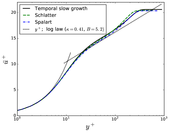
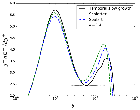
Figure 1: Mean streamwise velocity and its derivative, normalized by the viscous scales.

The mean velocity in the temporal DNS is qualitatively similar to that of both spatial simulations and follows closely the linear and logarithmic profiles. However, examining the quantity $\beta$ makes clear that there is not really a region over which the velocity varies logarithmically in any of the three simulations, because the Reynolds numbers are much too low. In channel flow, an order of magnitude larger Reynolds number was required to observe a significant logarithmic region (Lee & Moser, 2015). In the temporal case, the minimum of $\beta$ occurs with a value corresponding to $\kappa=0.41$, which is slightly larger than that observed for the spatial simulations. However, the simulations of Lee & Moser (2015) indicate that the value of $\kappa$ in an actual log layer at higher Reynolds number is likely to be significantly lower than this, since in the channel flow simulation, the minimum in $\beta$ is about 15% lower than the value in the log region.

Figure 2 shows the mean shear stress normalized by the wall shear stress.

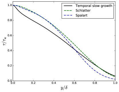
(a) Total shear stress.

(b) Viscous shear stress.

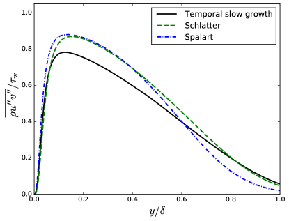
(c) Turbulent shear stress.

Figure 2: Shear stresses, normalized by the shear stress at the wall.

The shape of the total shear stress in the temporally homogenized boundary layer differs qualitatively from both the spatially homogenized and spatially evolving cases. In particular, as expected, the derivative of the total shear stress is zero at the wall in all cases, but the stress drops more quickly in the buffer layer in the temporally homogenized boundary layer. The mean viscous stress is essentially the same for the three different models, as expected given the mean velocity. Thus, the difference in the total stress is due to the Reynolds shear stress, with the peak value in the temporally homogenized simulation approximately 10% lower than in either of the spatial cases.

The observed differences in the behavior of the total shear stress can be explained by examining the relationship between the total stress and the mean velocity implied by the boundary layer approximation of the mean momentum equation. In particular, in a spatially evolving, zero-pressure-gradient, constant-density boundary layer, the boundary layer equations imply that the total shear stress is given by

$$\frac{\tau}{\tau_{\mathrm{w}}}=1+\frac{\nu}{u_{\tau}^{2}}\frac{\operatorname{d}\!u_{\tau}}{\operatorname{d}\!x}\int_{0}^{y^{+}}(u^{+})^{2}\operatorname{d}\!y^{+}.$$

Alternatively, the temporal slow growth formulation leads to

$$\frac{\tau}{\tau_{\mathrm{w}}}=1-\gamma(\Delta)^{+}\left[u^{+}y^{+}-\int_{0}^{y^{+}}u^{+}\operatorname{d}\!y^{+}\right],$$

where $\gamma(\Delta)^{+}=\nu\gamma(\Delta)/u_{\tau}^{2}$. These forms behave differently near the wall, leading to the discrepancies in total shear and Reynolds shear stress shown in Figure 2. For example, in the viscous sublayer where $u^{+}=y^{+}$, the spatially evolving result is $\tau/\tau_{\mathrm{w}}=1-C_{s}(y^{+})^{3}$, while the temporal slow growth boundary layer gives $\tau/\tau_{\mathrm{w}}=1-C_{t}(y^{+})^{2}$, where $C_{s}$ and $C_{t}$ are problem-dependent, positive constants. The temporal slow growth behavior in the viscous sublayer is consistent with a temporally evolving boundary layer—see Appendix B for more details—which leads to the observed discrepancies between the total stress in the current simulations and the spatially homogenized or evolving cases.

Figure 3 shows the RMS of the velocity fluctuations normalized by $u_{\tau}$.

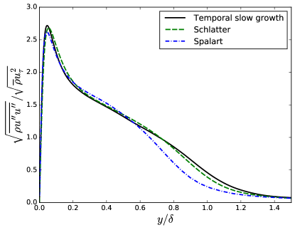
(a) Streamwise velocity RMS.

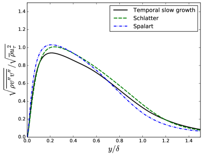
(b) Wall normal velocity RMS.

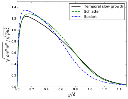
(c) Spanwise velocity RMS.

Figure 3: RMS velocity components.

As for the shear stresses, there is a reasonable agreement between the three simulations for the RMS velocities. The streamwise component shows particularly good agreement, with both the location and magnitude of the peak in close agreement between all three simulations. For the wall-normal and spanwise components, the temporal slow growth results tend to be below the spatial simulations, with the discrepancy near the peak being roughly 10%. Near the boundary layer edge, say for $y/\delta>0.8$, the temporal slow growth RMS velocities all agree better with the spatially evolving case than do the spatially homogenized profiles, although it is unclear why.

The turbulent kinetic energy budget is shown in Figure 4.

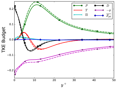
(a) Near wall region (non-dimensionalized by $u_{\tau}$ and $\nu/u_{\tau}$).

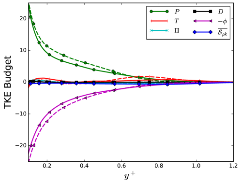
(b) Outer region (non-dimensionalized by $u_{\tau}$ and $\delta$).

Figure 4: Turbulent kinetic energy budget. Solid lines show results from the temporal slow growth approach. Dashed lines show results from spatial slow growth approach of Spalart (1988).

Specifically, using homogeneity in the streamwise ($x_{1}$) and spanwise ($x_{3}$) directions, the TKE equation can be written

$$\frac{\partial\bar{\rho}k}{\partial t}=C+P+T+\Pi+D-\phi+V+\overline{\mathcal{S}_{\rho k}},$$

where, in index notation,

$$C=-\,\tilde{u}_{2}\frac{\partial\rho k}{\partial x_{2}},\quad P=-\overline{\rho u^{\prime\prime}_{2}u^{\prime\prime}_{i}}\frac{\partial\tilde{u}_{i}}{\partial x_{2}},\quad T=-\,\frac{1}{2}\frac{\partial}{\partial x_{2}}\left(\overline{\rho u^{\prime\prime}_{i}u^{\prime\prime}_{i}u^{\prime\prime}_{2}}\right),$$

$$\Pi=-\,\frac{\partial}{\partial x_{2}}\left(\overline{u^{\prime\prime}_{2}p^{\prime}}\right)+\overline{p^{\prime}\frac{\partial u^{\prime\prime}_{i}}{\partial x_{2}}},\quad D=\frac{\partial}{\partial x_{2}}\left(\overline{u^{\prime\prime}_{i}\tau^{\prime}_{i2}}\right),\quad\phi=\overline{\tau^{\prime}_{ij}\frac{\partial u^{\prime\prime}_{i}}{\partial x_{j}}},$$

$$V=-\,\overline{u_{2}^{\prime\prime}}\frac{\partial\bar{p}}{\partial x_{2}}+\overline{u_{i}^{\prime\prime}}\frac{\partial\bar{\tau}_{ij}}{\partial x_{j}}-\bar{\rho}k\frac{\partial\tilde{u}_{2}}{\partial x_{2}},\quad\overline{\mathcal{S}_{\rho k}}=x_{2}\gamma(\Delta)\frac{\partial\bar{\rho}k}{\partial x_{2}}.$$

Because the density is essentially constant in this case, for the temporal formulation, $\tilde{u}_{2}\approx 0$, which implies that the mean convection term $\tilde{u}_{2}\partial(\bar{\rho}k)/\partial x_{2}$ is negligible. Further, the compressibility terms in $V$ are also negligible. Thus, only $P$, $T$, $\Pi$, $D$, $\phi$, and $\overline{\mathcal{S}_{\rho k}}$ are shown.

Near the wall, the features of the dominant terms in the TKE balance from the temporal slow growth simulation are similar to those from the spatial slow growth case. Both production and dissipation are somewhat smaller in the temporal case, which is consistent with the reduced Reynolds shear stress observed in Figure 2. The viscous and turbulent transport terms however match almost perfectly. Away from the wall, production and dissipation remain smaller in the temporal simulation, and the outer peak in the turbulent transport is significantly reduced.

To summarize, the temporal slow growth model flow mimics many of the important features of the statistics of a zero-pressure-gradient, spatially evolving boundary layer. The mean velocity, streamwise RMS velocity, and dominant near-wall terms in the $k$ budget are particularly well-represented. However, as expected, the differences between temporal and spatial evolution of the boundary layer and the approximations inherent to the slow-growth formulation lead to some obvious discrepancies. For instance, the Reynolds shear stress, wall-normal RMS velocity, and spanwise RMS velocity are all lower in the temporal simulation than in the spatially homogenized or spatially evolving cases. Such differences are relevant if the goal is to investigate the characteristics of a truly spatially evolving boundary layer; however, they do not diminish the utility of temporally homogenized boundary layers for studying wall-bounded turbulence more generally or for RANS model evaluation, as discussed in Section I.

III.2 Case (C): $M_{\infty}=1.2$, Cold Wall Boundary Layer with Transpiration

Results from the Case (C) simulation are presented and compared with those from the Case (L) in this section. Many of the statistics are normalized using the semi-local scaling introduced by Morinishi et al. (2004), where local mean viscosity and density are used in the friction velocity and viscous length scale rather than wall values. Hence, the semi-local friction velocity is $u_{\tau^{*}}=\sqrt{\tau_{\mathrm{w}}/\overline{\rho}}$, and the semi-local viscous length scale is $\delta_{\nu^{*}}=\overline{\mu}/(\overline{\rho}u_{\tau^{*}})$. The wall distance normalized by the semi-local viscous scale is denoted $y^{*}=y/\delta_{\nu^{*}}$. The use of this scaling has almost no effect on the Case (L) profiles. In Case (C), the use of this scaling is justified by the strong variation in density and viscosity near the wall due to the cold wall. As is evident in Figure 5, most of the variation in mean thermodynamic and transport quantities occurs in the viscous sublayer and buffer layer where $y^{*}\leq 20$.

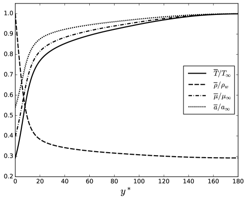
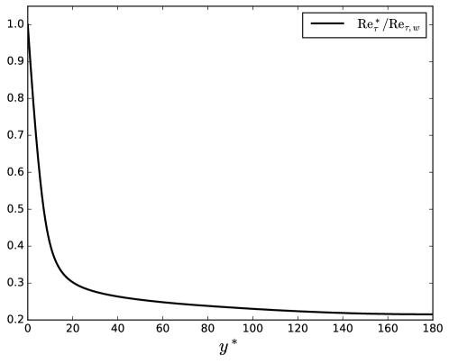
Figure 5: Variation of thermodynamic quantities and viscosity as a function of wall distance normalized by the semi-local length scale (top) and ratio of Reynolds number based on semi-local friction velocity, boundary layer thickness, and local kinematic viscosity relative to Reynolds number based on friction velocity, boundary layer thickness, and wall kinematic viscosity.

This strong variation in mean properties leads to a large variation in local Reynolds number across the boundary layer, with the near-wall region having the highest Re based on local properties.

While the thermodynamic and transport properties vary dramatically, the turbulent Mach number $M_{t}=\sqrt{\widetilde{u^{\prime\prime}_{i}u^{\prime\prime}_{i}}}/\overline{a}$, shown in Figure 6, is low, with a maximum of approximately 0.2, as expected in a mildly supersonic boundary layer.

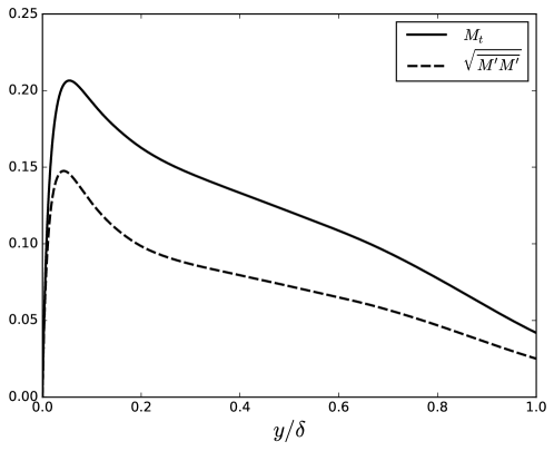
Figure 6: Turbulent Mach number and Mach number RMS.

Therefore, according to Morkovin’s hypothesis (Morkovin, 1962; Smits & Dussauge, 2006), it is expected that the effects of compressibility on turbulence are very weak for this case, although the property variations will cause the results to differ substantially from a low Mach boundary layer.

Figure 7 shows the mean velocity for Case (C).

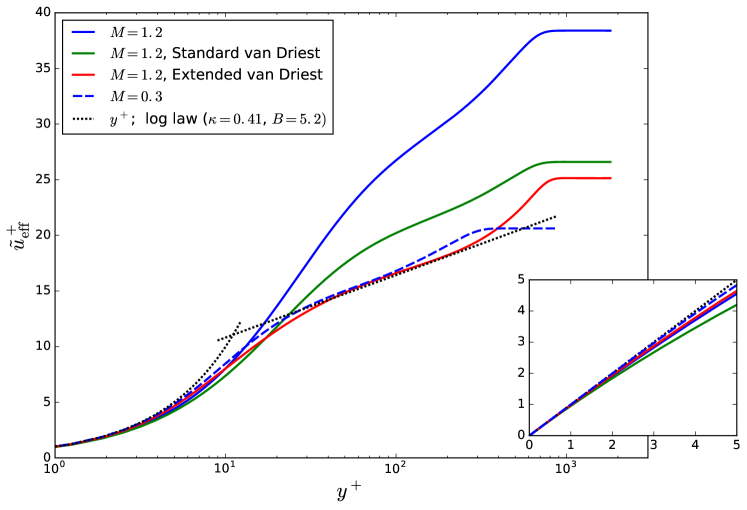
Figure 7: Mean streamwise velocity. Five profiles are shown: The raw Case (C) profile (solid blue), the van Driest transformed Case (C) profile (solid green), the extended van Driest transformed (see Appendix C) Case (C) profile (solid red), the Case (L) profile (dashed blue), and the law of the wall (dotted black). The inset shows the viscous sublayer only.

Three different transformations of the Case (C) streamwise mean velocity are shown. The first, shown in blue, is simply the mean velocity normalized by the friction velocity. Of course, this normalization does not account for variable property effects and, as expected, the result does not collapse on the Case (L) profile (blue dashed line) or the incompressible law of the wall (black dotted line). It is common practice to consider the van Driest (1951) transformed mean velocity when comparing compressible boundary layers to their incompressible counterparts, and this transformation is often successful in collapsing the profiles (White, 1991). The van Driest transformed velocity is shown in Figure 7 in green. While this profile is closer to the incompressible velocity profile than the untransformed velocity, there are still substantial discrepancies. First, the transformed velocity is below the $u^{+}=y^{+}$ curve for $y^{+}$ less than 3, as is clear in the inset of Figure 7. Second, there is a large offset in the log layer, which would lead to a log layer offset constant greater than 10. These discrepancies can be explained by the fact that the transformation does not account for the effects of wall transpiration or a highly cooled wall. The effects of the cold wall have been previously examined by Huang & Coleman (1994), who proposed a modified transformation that accounts for the temperature variation in the viscous sublayer. In Appendix C, we develop a further extension of the transformation of Huang & Coleman (1994) that accounts for both the cold wall and wall transpiration. The result of applying this transformation is shown in red in Figure 7. The transformation is quite successful in collapsing the Case (C) velocity profile with incompressible theory, indicating that mean property variation accounts for the differences between the compressible and incompressible mean velocity profiles for this case.

Figure 8 shows the shear stresses.

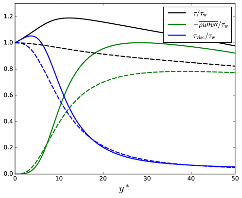
(a) Inner region.

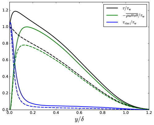
(b) Entire boundary layer.

Figure 8: Shear stress components, normalized by the wall stress. The solid lines represent Case (C) while the dashed lines are from Case (L).

Unlike Case (L), the total shear stress has a positive derivative at the wall and peaks near $y^{*}\approx 12$ with a value approximately $20\%$ larger than at the wall. These features are a consequence of the wall transpiration. With wall transpiration, the term $\bar{\rho}\tilde{v}\partial\tilde{u}/\partial y$ in the mean momentum equation, which is zero at the wall and negligible near the wall in the non-blowing case, is non-zero even at the wall. This term leads to a larger total shear over the entire boundary layer, which, outside of the viscous sublayer, leads to a larger Reynolds shear stress. In particular, at its peak, the Reynolds shear stress is also approximately $20\%$ larger in Case (C) than in Case (L).

The effects of wall transpiration can also be seen in the RMS velocities (Figure 9).

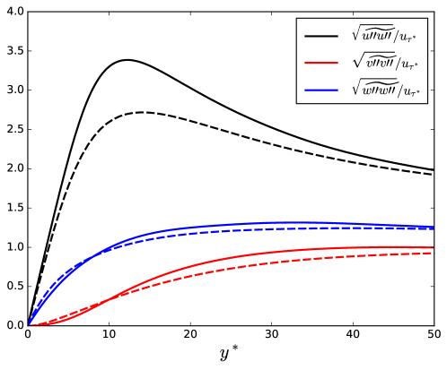
(a) Inner region.

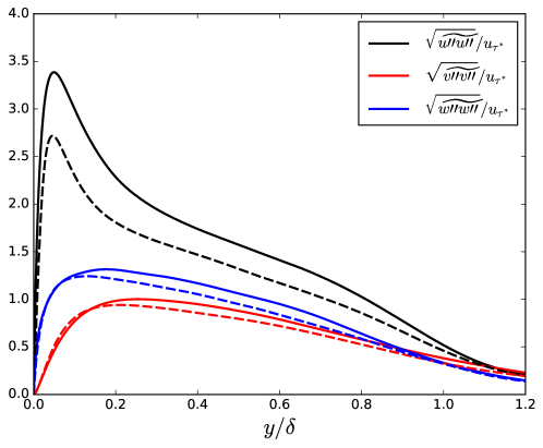
(b) Entire boundary layer.

Figure 9: RMS velocities, normalized by the semi-local friction velocity. The solid lines represent Case (C) while the dashed lines are from Case (L).

The streamwise RMS velocity component in particular is greatly enhanced by wall transpiration, increasing by approximately $30\%$ from Case (L) to Case (C). These observations are consistent with the results obtained by Sumitani & Kasagi (1995) for a channel flow with an injecting wall and a suction wall. They showed that turbulent fluctuations are larger on the injection side as compared with a channel with an impermeable wall.

To examine the Reynolds heat flux, Figure 10 shows the turbulent Prandtl number:

$$\mbox{Pr}_{t}=\frac{\overline{\rho u^{\prime\prime}v^{\prime\prime}}(\partial\widetilde{T}/\partial y)}{\overline{\rho T^{\prime\prime}v^{\prime\prime}}(\partial\widetilde{u}/\partial y)}.$$

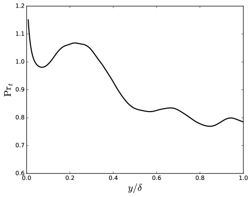
Figure 10: Turbulent Prandtl number.

In standard RANS modeling, $\mbox{Pr}_{t}$ is taken to be a constant, usually $\mbox{Pr}_{t}=0.9$, although values between $0.6$ and $1.0$ have been used. Examining the figure, it is clear that, while the standard value of $\mbox{Pr}_{t}\approx 0.9$ is a reasonable compromise for this case, the true value varies substantially across the boundary layer, from $\mbox{Pr}_{t}\approx 0.8$ to greater than $1.1$ near the wall. Similar values and trends for $\mbox{Pr}_{t}$ were also observed by Guarini et al. (2000) and Pirozzoli et al. (2004) in adiabatic, impermeable wall simulations, indicating that the accuracy of the constant $\mbox{Pr}_{t}$ approximation does not substantially degrade due to cold wall or blowing effects.

Finally, the turbulent kinetic energy budget is shown in Figure 11.

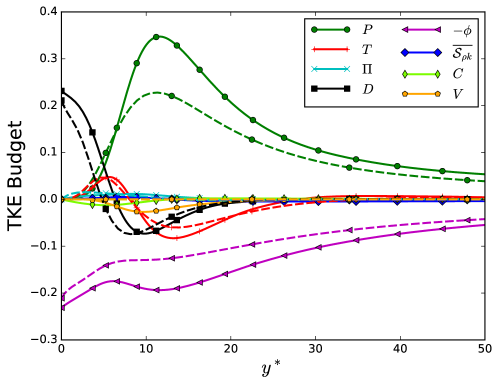
(a) Near wall region (non-dimensionalized by semi-local scales).

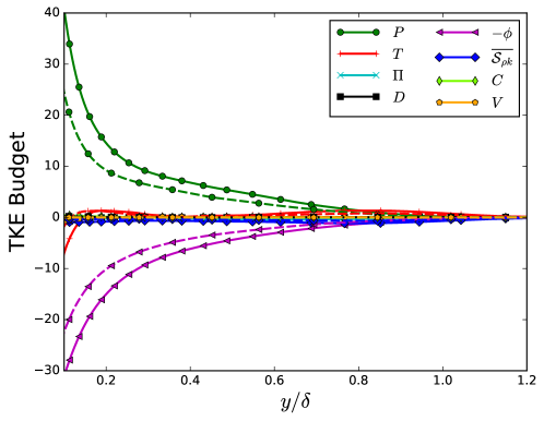
(b) Outer region (non-dimensionalized by $\delta$, $\bar{\rho}$, and $u_{\tau^{*}}$).

Figure 11: Turbulent kinetic energy budget. Solid lines show results from Case (C). Dashed lines show results from Case (L).

Unlike the budget profiles of Guarini et al. (2000), which collapsed reasonably well with those from the incompressible simulations of Spalart (1988) when non-dimensionalized using $u_{\tau}$ and $\nu_{\mathrm{w}}$, the budget for Case (C) is substantially different than that for Case (L). The near-wall peak in production for Case (C) is almost $50\%$ greater than the peak production in Case (L), which is consistent with the enhanced Reynolds stress due to blowing. The dissipation and turbulent transport are also larger in magnitude in the near-wall region for Case (C) relative to Case (L). Further, neither the mean convection $C$ nor the terms associated with variable density $V$ are entirely negligible.

IV Conclusions

A new slow growth formulation for DNS of wall-bounded turbulence has been developed and used to simulate two flows: an essentially incompressible boundary layer and a transonic boundary layer over a cooled wall with transpiration. Like previous slow growth approaches, the new formulation relies on an assumption that the mean and RMS quantities evolve slowly relative to the turbulent fluctuations. This assumption is used to develop a set of governing equations for the fast evolution of the turbulent fluctuations subject to forcing from the slow evolution of the mean and RMS. After modeling the impact of the slow evolution in this scenario, one can simulate the fast evolution at a fixed point in the slow development.

Unlike previous approaches, the present model is developed based on a temporally evolving boundary layer. Furthermore, the current approach is specifically designed to enable calibration and validation of RANS-based turbulence models for complex boundary layer flows. It is formulated to ensure that the slow growth sources that appear in the RANS equations are closed in terms of the RANS variables. This avoids any potential confounding of errors between typical RANS closures and new modeling required to close the mean slow growth sources. Further, the slow growth source terms that arise from the homogenization procedure are modeled assuming a self-similar evolution of mean and RMS profiles. This procedure allows straightforward extensions to cases involving other physical phenomena such as compressibility, transpiration and chemical reactions, which have not been addressed in previous slow growth formulations.

The results show that in the incompressible case the results display many characteristics associated with typical boundary layer turbulence. The mean velocity profile has the typical structure, and the streamwise RMS velocity peak location and magnitude is consistent with other simulations. Other statistics, most notably the total shear stress and Reynolds shear stress, display notable discrepancies with spatial simulations. These discrepancies result from the difference between the temporal slow growth model and the true slow evolution of a spatially evolving boundary layer, due both to the temporal evolution and the slow growth approximations. This observation points to the possibility that an improved slow growth model could reduce this discrepancy and give a better representation of a spatially developing flow. While beyond the scope of this paper, such models have been proposed (Ulerich, 2014) and remedy some of the differences observed here. Nonetheless, despite the mild discrepancies between the current slow growth formulation and spatially evolving boundary layers, the slow growth simulations are a valuable resource for evaluation of RANS models. Specifically, the slow growth boundary layer is sufficiently similar to a spatially evolving one that a model that represents the former should be able to simulate the later.

Finally, the transonic, cold wall case with wall transpiration shows that the approach can be straightforwardly extended to problems with more complex physics. This capability is significant because it enables the development of data sets for assessing the validity of lower fidelity models, namely RANS models, in the presence of these complicating phenomena. This is particularly useful for calibration and validation because reliable data for boundary layers with such complications is often scarce or nonexistent. Work to further extend the slow growth capability to treat pressure gradients and reacting flows is underway. These capabilities together will enable affordable DNS of boundary layer flows similar to those observed on vehicles during atmospheric entry and in other complex systems.

Appendix A An inconsistent slow growth formulation

A straightforward formulation can be obtained by considering a Reynolds decomposition of the conserved variables. Specifically, let

$$\rho q\!\left(x,y,z,t\right)=\overline{\rho q}\!\left(y,t_{s}\right)+\underbrace{A_{\rho q}\!\left(y,t_{s}\right)\rho q^{\prime}_{p}\!\left(x,y,z,t_{f}\right)}_{\rho q^{\prime}\!\left(x,y,z,t_{f},t_{s}\right)},$$

where the mean $\overline{\rho q}$ and amplitude function $A_{\rho q}$ are assumed to evolve only in slow time. As in Section II.3, to model the slow time derivatives, the mean and amplitude are assumed to evolve in time in a self-similar manner:

$$\overline{\rho q}\!\left(t_{s},y\right) =F_{\rho q}\!\left(y/\Delta(t_{s})\right),$$

$$A_{\rho q}\!\left(t_{s},y\right) =G_{\rho q}\!\left(y/\Delta(t_{s})\right).$$

Then, by an exactly analogous development to that shown in Section II.3, the slow growth source for $\rho q$ is found to be

$$\mathcal{S}_{\rho q}=y\,\gamma(\Delta)\left(\frac{\partial\overline{\rho q}}{\partial y}+\frac{(\rho q)^{\prime}}{A_{\rho q}}\frac{\partial A_{\rho q}}{\partial y}\right).$$

Without specifying $A_{\rho q}$, it is clear that, while the mean of $\mathcal{S}_{\rho q}$ is closed in terms of the mean flow, the mean of the slow growth source in the TKE equation cannot be closed without additional modeling in this formulation. Thus, the formulation is discarded in favor of that shown in Section II.3. Nonetheless, we have performed simulations using this formulation, and it leads to similar results to those presented in this work. This observation indicates that the results are not highly sensitive to the choice of whether to apply the Reynolds decomposition to the primitive or conserved variables.

Appendix B Analysis of Total Stress

In this section, we examine the relationship between the mean streamwise velocity and the total stress in a spatially evolving boundary layer, a temporally evolving boundary layer, and the temporal slow growth model. In particular, we consider a zero-pressure-gradient, constant-density boundary layer flow and analyze the appropriate form of the boundary layer equations for each case. The implied behavior of the total stress for the different cases explains the near wall differences observed in the total stress profiles shown in Section III.1.

B.1 Spatially Evolving Boundary Layer

For the spatially evolving case, the mean boundary layer equations can be written

$$\frac{\partial u}{\partial x}+\frac{\partial v}{\partial y}=0,$$

$$u\frac{\partial u}{\partial x}+v\frac{\partial u}{\partial y}=\frac{\partial\tau}{\partial y},$$

where $x$ is the streamwise direction, $y$ is the wall-normal direction, $u$ and $v$ are the mean streamwise and wall-normal velocities, respectively, and $\tau$ is the mean total shear stress. Assuming that the streamwise velocity normalized by the friction velocity is only a function of wall-normal distance normalized by the viscous length scale, i.e., $u(x,y)/u_{\tau}(x)=u^{+}(y^{+})$, one can derive a relationship between the total shear stress and the velocity. To begin, note that

$$u=u_{\tau}(x)\,u^{+}(y^{+})\quad\Rightarrow\quad\frac{\partial u}{\partial x}=\frac{\operatorname{d}\!u_{\tau}}{\operatorname{d}\!x}\left(u^{+}+y^{+}\frac{\operatorname{d}\!u^{+}}{\operatorname{d}\!y^{+}}\right)=\frac{\operatorname{d}\!u_{\tau}}{\operatorname{d}\!x}\,\frac{\operatorname{d}\!missing}{\operatorname{d}\!y^{+}}\left(y^{+}u^{+}\right).$$

Thus, the wall-normal velocity is given by

$$v(x,y)=-\int_{0}^{y}\frac{\partial u}{\partial x}dy=-\int_{0}^{y^{+}}\frac{\operatorname{d}\!u_{\tau}}{\operatorname{d}\!x}\,\frac{\operatorname{d}\!missing}{\operatorname{d}\!y^{+}}\left(y^{+}u^{+}\right)\frac{\nu}{u_{\tau}}\,dy^{+}=-\,\frac{\nu}{u_{\tau}}\frac{\operatorname{d}\!u_{\tau}}{\operatorname{d}\!x}y^{+}u^{+}.$$

Using these results to evaluate the convection term in the mean momentum equation gives

$$u\frac{\partial u}{\partial x}=u_{\tau}\frac{\operatorname{d}\!u_{\tau}}{\operatorname{d}\!x}\,u^{+}\frac{\operatorname{d}\!missing}{\operatorname{d}\!y^{+}}\left(y^{+}u^{+}\right),$$

$$v\frac{\partial u}{\partial y}=-\frac{\operatorname{d}\!u_{\tau}}{\operatorname{d}\!x}y^{+}u^{+}\frac{\nu}{u_{\tau}}u_{\tau}\frac{\operatorname{d}\!u^{+}}{\operatorname{d}\!y^{+}}\frac{u_{\tau}}{\nu}=-u_{\tau}\frac{\operatorname{d}\!u_{\tau}}{\operatorname{d}\!x}y^{+}u^{+}\frac{\operatorname{d}\!u^{+}}{\operatorname{d}\!y^{+}}.$$

Thus,

$$u\frac{\partial u}{\partial x}+v\frac{\partial u}{\partial y}=u_{\tau}\frac{\operatorname{d}\!u_{\tau}}{\operatorname{d}\!x}\left(u^{+}\frac{\operatorname{d}\!missing}{\operatorname{d}\!y^{+}}\left(y^{+}u^{+}\right)-y^{+}u^{+}\frac{\operatorname{d}\!u^{+}}{\operatorname{d}\!y^{+}}\right)=u_{\tau}\frac{\operatorname{d}\!u_{\tau}}{\operatorname{d}\!x}(u^{+})^{2}.$$

Substituting into the mean momentum equation gives

$$u_{\tau}\frac{\operatorname{d}\!u_{\tau}}{\operatorname{d}\!x}(u^{+})^{2}=\frac{\partial\tau}{\partial y}.$$

Thus,

$$\tau-\tau_{\mathrm{w}}=\int_{0}^{y}\frac{\partial\tau}{\partial y}dy=u_{\tau}\frac{\operatorname{d}\!u_{\tau}}{\operatorname{d}\!x}\int_{0}^{y}(u^{+})^{2}\operatorname{d}\!y.$$

Finally, non-dimensionalizing by $\nu$ and $u_{\tau}$ gives

$$\frac{\tau}{\tau_{\mathrm{w}}}=1+\left(\frac{\nu}{u_{\tau}^{2}}\frac{\operatorname{d}\!u_{\tau}}{\operatorname{d}\!x}\right)\int_{0}^{y^{+}}(u^{+})^{2}\,\operatorname{d}\!y^{+}.$$

B.2 Temporally Evolving Boundary Layer

In the temporally evolving case, the flow is necessarily homogeneous in the streamwise direction. Conservation of mass plus the no slip condition implies that $v=0$. Thus, the boundary layer equations reduce to

$$\frac{\partial u}{\partial t}=\frac{\partial\tau}{\partial y}.$$

As in the spatially evolving case, we assume that $u^{+}$ is a universal function of $y^{+}$ only. Then,

$$\frac{\partial u}{\partial t}=\frac{\operatorname{d}\!u_{\tau}}{\operatorname{d}\!t}u^{+}+y^{+}\frac{\operatorname{d}\!u^{+}}{\operatorname{d}\!y^{+}}\frac{\operatorname{d}\!u_{\tau}}{\operatorname{d}\!t}=\frac{\operatorname{d}\!u_{\tau}}{\operatorname{d}\!t}\frac{\operatorname{d}\!\,(u^{+}y^{+})}{\operatorname{d}\!y^{+}}.$$

Substituting this result into mean momentum and integrating gives

$$\tau-\tau_{\mathrm{w}}=\int_{0}^{y}\frac{\partial\tau}{\partial y}\operatorname{d}\!y=\frac{\nu}{u_{\tau}}\frac{\operatorname{d}\!u_{\tau}}{\operatorname{d}\!t}\,(u^{+}y^{+}).$$

Thus, non-dimensionalizing using $\nu$ and $u_{\tau}$ gives

$$\frac{\tau}{\tau_{\mathrm{w}}}=1+\left(\frac{\nu}{u_{\tau}^{3}}\frac{\operatorname{d}\!u_{\tau}}{\operatorname{d}\!t}\right)(u^{+}y^{+}).$$

B.3 Temporal Slow Growth Boundary Layer

The temporal slow growth solution is also homogeneous in the streamwise direction, which leads to $v=0$, as in the temporally evolving case. In addition, the flow is statistically stationary by design. Thus, the boundary layer equations become

$$0=\frac{\partial\tau}{\partial y}+\overline{S_{u}},$$

where

$$\overline{S_{u}}=y\,\gamma(\Delta)\frac{\partial u}{\partial y}.$$

Thus,

$$\tau=\tau_{\mathrm{w}}-\gamma(\Delta)\left[uy-\int_{0}^{y}u\operatorname{d}\!y\right],$$

and

$$\frac{\tau}{\tau_{\mathrm{w}}}=1-\left(\frac{\nu}{u_{\tau}^{2}}\gamma(\Delta)\right)\left[u^{+}y^{+}-\int_{0}^{y^{+}}u^{+}\operatorname{d}\!y^{+}\right].$$

Appendix C An Extended Van Driest Transformation

We construct an extension of the van Driest transformation that accounts for the effects of wall transpiration and wall cooling. The van Driest transformation (van Driest, 1951) is derived using the following relationship between the compressible mean velocity ($\tilde{u}$) and the incompressible mean velocity ($\bar{u}_{\mathrm{inc}}$):

$$\frac{\operatorname{d}\!\tilde{u}^{+}}{\operatorname{d}\!y^{+}}=\frac{(\bar{\rho}/\bar{\rho}_{\mathrm{w}})^{1/2}}{\kappa y^{+}}=\left(\frac{\bar{\rho}}{\bar{\rho}_{\mathrm{w}}}\right)^{1/2}\frac{\operatorname{d}\!\bar{u}^{+}_{\mathrm{inc}}}{\operatorname{d}\!y^{+}},$$ (29)

which is valid in the log layer. As pointed out by Huang & Coleman (1994), in the viscous sublayer, (29) is incorrect. Instead, in the sublayer, the correct relationship is

$$\frac{\operatorname{d}\!\tilde{u}^{+}}{\operatorname{d}\!y^{+}}=\frac{\mu_{\mathrm{w}}}{\mu}\frac{\operatorname{d}\!\bar{u}^{+}_{\mathrm{inc}}}{\operatorname{d}\!y^{+}}.$$

The van Driest transformation is derived by integrating (29) starting at the wall, without any correction for the viscous sublayer. Strictly speaking, this procedure is always incorrect, but as long as the temperature does not vary dramatically in the viscous sublayer, the difference between $(\mu_{\mathrm{w}}/\mu)$ and $(\bar{\rho}/\bar{\rho}_{\mathrm{w}})^{1/2}$ is not large, and the resulting transformed velocity profile agrees well with incompressible results (White, 1991). However, when the temperature variation in the sublayer is large, as it is for a cold wall as shown in Section III.2, the error due to the sublayer is large enough that the collapse between the transformed profile and the incompressible results is quite poor.

To remedy this error, Huang & Coleman (1994) proposed a blending between the viscous sublayer and log layer results based on an assumed mixing length. Here, this approach is extended to include the effect of wall transpiration. The primary effect of wall transpiration is that the wall normal mean convection term in the mean momentum equation is no longer negligible near the wall. Thus, rather than containing only the viscous and Reynolds shear stresses, the total shear stress contains a contribution from wall-normal convection. Using the boundary layer form of the slow growth mean momentum equation, one can show that

$$\bar{\rho}\tilde{u}\tilde{v}=\tau-\tau_{\mathrm{w}}+\int_{0}^{y}\overline{\mathcal{S}_{\rho u}}\operatorname{d}\!y.$$

An analogous development can be done for the spatially developing case. For brevity, this analysis is not shown since only the slow growth version is used here.

Since $\tau=\mu\partial\tilde{u}/\partial y-\overline{\rho u^{\prime\prime}v^{\prime\prime}}$ (where $\mu$ is the mean viscosity and we have neglected the viscosity/velocity gradient correlation), the wall shear stress can be written as

$$\tau_{\mathrm{w}}=-\bar{\rho}\tilde{u}\tilde{v}+\int_{0}^{y}\overline{\mathcal{S}_{\rho u}}\operatorname{d}\!y+\mu\frac{\partial\tilde{u}}{\partial y}-\overline{\rho u^{\prime\prime}v^{\prime\prime}}.$$ (30)

To simplify notation, the convection and slow growth source terms can be grouped together. Note that

$$\int_{0}^{y}\overline{\mathcal{S}_{\rho u}}=\int_{0}^{y}y\gamma(\Delta)\frac{\partial\overline{\rho u}}{\partial y}=y\gamma(\Delta)\overline{\rho u}-\gamma(\Delta)\int_{0}^{y}\overline{\rho u}.$$

Thus,

$$\bar{\rho}\tilde{u}\tilde{v}-\int_{0}^{y}\overline{\mathcal{S}_{\rho u}}\operatorname{d}\!y=\bar{\rho}\tilde{u}\left(\tilde{v}-y\gamma(\Delta)+\gamma(\Delta)\int_{0}^{y}\frac{\overline{\rho u}(\eta)}{\overline{\rho u}(y)}\,\operatorname{d}\!\eta\right).$$

Then, let

$$\tilde{v}_{\mathrm{mod}}=\tilde{v}-y\gamma(\Delta)+\gamma(\Delta)\int_{0}^{y}\frac{\overline{\rho u}(\eta)}{\overline{\rho u}(y)}\,\operatorname{d}\!\eta.$$

With this notation, (30) can be rewritten as

$$\tau_{\mathrm{w}}=-\bar{\rho}\tilde{u}\tilde{v}_{\mathrm{mod}}+\mu\frac{\partial\tilde{u}}{\partial y}-\overline{\rho u^{\prime\prime}v^{\prime\prime}}.$$ (31)

To continue, we use a mixing length model for the Reynolds stress:

$$-\overline{\rho v^{\prime\prime}u^{\prime\prime}}=\bar{\rho}\ell^{2}\left(\frac{\partial\tilde{u}}{\partial y}\right)^{2}.$$

Then, (31) can be rewritten as

$$\tau_{\mathrm{w}}=-\bar{\rho}\tilde{v}_{\mathrm{mod}}\tilde{u}+\mu\frac{\partial\tilde{u}}{\partial y}+\bar{\rho}\ell^{2}\left(\frac{\partial\tilde{u}}{\partial y}\right)^{2}.$$

Solving this quadratic for $\partial\tilde{u}/\partial y$, one obtains

$$\frac{\partial\tilde{u}}{\partial y}=\frac{2\left(\bar{\rho}\tilde{v}_{\mathrm{mod}}\tilde{u}+\tau_{\mathrm{w}}\right)}{\mu+\sqrt{\mu^{2}+4\bar{\rho}\ell^{2}\left(\bar{\rho}\tilde{v}_{\mathrm{mod}}\tilde{u}+\tau_{\mathrm{w}}\right)}}\,.$$

Non-dimensionalizing this result using $\rho_{\mathrm{w}}$, $\mu_{\mathrm{w}}$, and $u_{\tau}$ gives

$$\frac{\partial\tilde{u}^{+}}{\partial y^{+}}=\frac{2\left(\hat{\rho}\tilde{v}_{\mathrm{mod}}^{+}\tilde{u}^{+}+1\right)}{\hat{\mu}^{2}+\sqrt{\hat{\mu}^{2}+4\hat{\rho}(\ell^{+})^{2}\left(\hat{\rho}\tilde{v}_{\mathrm{mod}}^{+}\tilde{u}^{+}+1\right)}}\,,$$ (32)

where $\hat{\rho}=\bar{\rho}/\rho_{\mathrm{w}}$, $\hat{\mu}=\mu/\mu_{\mathrm{w}}$, and $\ell^{+}=\rho_{\mathrm{w}}u_{\tau}\ell/\mu_{\mathrm{w}}$. In the incompressible, non-blowing wall case, this result simplifies to

$$\frac{\partial\bar{u}_{\mathrm{inc}}^{+}}{\partial y^{+}}=\frac{2}{1+\sqrt{1+4(\ell_{\mathrm{inc}}^{+})^{2}}},$$ (33)

where $\ell_{\mathrm{inc}}$ is the mixing length for the incompressible case.

The extended van Driest transformation is obtained by requiring that the nondimensional transformed velocity $\tilde{u}_{\mathrm{eff}}^{+}$ has the same profile as the incompressible velocity. That is,

$$\tilde{u}_{\mathrm{eff}}^{+}(\tilde{u}^{+}(y^{+}))=\bar{u}^{+}_{\mathrm{inc}}(y^{+}),$$

which implies that

$$\frac{\operatorname{d}\!\tilde{u}_{\mathrm{eff}}^{+}}{\operatorname{d}\!\tilde{u}^{+}}\,\frac{\operatorname{d}\!\tilde{u}^{+}}{\operatorname{d}\!y^{+}}=\frac{\operatorname{d}\!\bar{u}_{\mathrm{inc}}^{+}}{\operatorname{d}\!y^{+}}.$$

Thus,

$$\tilde{u}_{\mathrm{eff}}^{+}(w^{+})=\int_{0}^{w^{+}}\frac{\operatorname{d}\!\tilde{u}_{\mathrm{eff}}^{+}}{\operatorname{d}\!\tilde{u}^{+}}\,\operatorname{d}\!\tilde{u}^{+}=\int_{0}^{w^{+}}\frac{\operatorname{d}\!\bar{u}_{\mathrm{inc}}^{+}/\operatorname{d}\!y^{+}}{\operatorname{d}\!\tilde{u}^{+}/\operatorname{d}\!y^{+}}\,\operatorname{d}\!\tilde{u}^{+}.$$ (34)

Substituting (32) and (33) into (34) gives

$$\tilde{u}_{\mathrm{eff}}^{+}(w^{+})=\bigintss_{0}^{w^{+}}\frac{\hat{\mu}+\sqrt{\hat{\mu}^{2}+4\hat{\rho}(\ell^{+})^{2}\left(\hat{\rho}\tilde{v}_{\mathrm{mod}}^{+}\tilde{u}^{+}+1\right)}}{(\hat{\rho}\tilde{v}_{\mathrm{mod}}^{+}\tilde{u}^{+}+1)\left(\sqrt{1+4(\ell_{\mathrm{inc}}^{+})^{2}}+1\right)}\,\operatorname{d}\!\tilde{u}^{+}.$$ (35)

To complete the transformation, one must define the mixing length. We use the van Driest damping (van Driest, 1956) function:

$$\ell^{+}=\kappa y^{+}\left(1-\exp(-y^{*}/A^{+})\right),$$

$$\ell_{\mathrm{inc}}^{+}=\kappa y^{+}\left(1-\exp(-y^{+}/A^{+})\right),$$

where the wall-distance normalized by the semi-local viscous length is used in the compressible case. We take typical values of the parameters: $\kappa=0.41$ and $A^{+}=25.51$.

At this point, if profiles for $\hat{\rho}$, $\hat{\mu}$, $\tilde{v}_{\mathrm{mod}}^{+}$ and $\tilde{u}^{+}$ are available, (35) allows computation of the equivalent incompressible profile. Thus, this form is appropriate for data analysis, and it is used for this purpose in Section III.2. However, it does not give a closed form for modeling a compressible profile. For this task, a model temperature profile is required. See Huang & Coleman (1994) for an example.

To conclude, we examine how the extended transformation compares to existing transformations. When $\tilde{v}_{\mathrm{mod}}^{+}$ is negligible (i.e., no wall transpiration or slow growth), the transformation reduces to the method of Huang & Coleman (1994), which itself reduces to the standard van Driest transformation outside the viscous sublayer. Alternatively, for the incompressible case with wall transpiration, the extended transformation in the log layer reduces to the log layer correction for injection effects derived by Stevenson (1963).

References

- Bauman et al. (2011) Bauman, Paul T., Stogner, Roy, Carey, Graham F., Schulz, Karl W., Upadhyay, Rochan & Maurente, Andre 2011 Loose-coupling algorithm for simulating hypersonic flows with radiation and ablation. Journal of Spacecraft and Rockets 48 (1), 72––80.
- Guarini et al. (2000) Guarini, S.E., Moser, R.D., Shariff, K. & Wray, A. 2000 Direct numerical simulation of a supersonic turbulent boundary layer at Mach 2.5. Journal of Fluid Mechanics 414, 1–33.
- Huang & Coleman (1994) Huang, PG & Coleman, Gary N 1994 Van Driest transformation and compressible wall-bounded flows. AIAA Journal 32 (10), 2110–2113.
- Huang et al. (1995) Huang, P. G., Coleman, G. N. & Bradshaw, P. 1995 Compressible turbulent channel flows: DNS results and modeling. Journal of Fluid Mechanics 305, 185–218.
- Jewkes et al. (2011) Jewkes, J. W., Chung, Y. M. & Carpenter, P. W. 2011 Modifications to a turbulent inflow generation method for boundary-layer flows. AIAA Journal 49 (1), 247–250.
- Kirk et al. (2014) Kirk, B. S., Stogner, R. H., Bauman, P. T. & Oliver, T. A. 2014 Modeling hypersonic entry with the Fully-Implicit Navier-Stokes (FIN-S) stabilized finite element flow solver. Computers and Fluids 92, 281–292.
- Lee & Moser (2015) Lee, Myoungkyu & Moser, Robert D. 2015 Direct numerical simulation of turbulent channel flow up to . Journal of Fluid Mechanics 774, 395–415.
- Lund et al. (1998) Lund, T. S., Wu, X. & Squires, K. D. 1998 Generation of turbulent inflow data for spatially-developing boundary layer simulations. Journal of Computational Physics 140, 233–258.
- Morinishi et al. (2004) Morinishi, Y, Tamano, S & Nakabayashi, K 2004 Direct numerical simulation of compressible turbulent channel flow between adiabatic and isothermal walls. Journal of Fluid Mechanics 502, 273–308.
- Morkovin (1962) Morkovin, Mark V 1962 Effects of compressibility on turbulent flows. Mécanique de la Turbulence pp. 367–380.
- Nikitin (2007) Nikitin, N. 2007 Spatial periodicity of spatially evolving turbuleent flow caused by inflow boundary condition. Physics of Fluids 19, 091703.
- Pirozzoli et al. (2004) Pirozzoli, S., Grasso, F. & Gatski, T. B. 2004 Direct numerical simulation and analysis of a spatially evolving supersonic turbulent boundary layer at . Physics of Fluids 16 (3), 530–545.
- Schlatter & Örlü (2010) Schlatter, Philipp & Örlü, Ramis 2010 Assessment of direct numerical simulation data of turbulent boundary layers. Journal of Fluid Mechanics 659, 116–126.
- Sillero et al. (2013) Sillero, Juan A., Jimenez, Javier & Moser, Robert D. 2013 One-point statistics for turbulent wall-bounded flows at reynolds numbers up to . Physics of Fluids 25, 105102.
- Sinha & Candler (2003) Sinha, Krishnendu & Candler, Graham 2003 Turbulent dissipation-rate equation for compressible flows. AIAA Journal 41 (6), 1017–1021.
- Smits & Dussauge (2006) Smits, Alexander J. & Dussauge, Jean-Paul 2006 Turbulent Shear Layers in Supersonic Flow. Springer.
- Spalart (1986) Spalart, P. R. 1986 Numerical study of sink-flow boundary layers. Journal of Fluid Mechanics 172, 302–328.
- Spalart (1988) Spalart, Philippe R. 1988 Direct simulation of a turbulent boundary layer up to Reθ =1410. Journal of Fluid Mechanics 187, 61–98.
- Spalart & Leonard (1985) Spalart, P. R. & Leonard, A. 1985 Direct numerical simulation of equilibrium turbulent boundary layers. Proc. 5th Symp. on Turbulent Shear Flows, Ithaca, NY, August 7–9, 1985.
- Stevenson (1963) Stevenson, TN 1963 A law of the wall for turbulent boundary layers with suction or injection. CoA Report Aero 166. The College of Aeronautics Cranfield.
- Stogner et al. (2011) Stogner, Roy, Bauman, Paul T., Schulz, Karl W., Upadhyay, Rochan & Maurente, Andre 2011 Uncertainty and parameter sensitivity in multiphysics reentry flows. In 49th AIAA Aerospace Sciences Meeting including the New Horizons Forum and Aerospace Exposition (Paper No. 2011-764).
- Sumitani & Kasagi (1995) Sumitani, Yasushi & Kasagi, Nobuhide 1995 Direct numerical simulation of turbulent transport with uniform wall injection and suction. AIAA Journal 33 (7), 1220–1228.
- Ulerich (2014) Ulerich, Rhys 2014 Reducing turbulence- and transition-driven uncertainty in aerothermodynamic heating predictions for blunt-bodied reentry vehicles. PhD thesis, The University of Texas at Austin.
- van Driest (1951) van Driest, E. R. 1951 Turbulent boundary layers in compressible fluids. Journal of Aeronautical Sciences 18 (3).
- van Driest (1956) van Driest, E. R. 1956 On turbulent flow near a wall. Journal of Aeronautical Sciences 23.
- White (1991) White, F. M. 1991 Viscous Fluid Flow, Second Edition. New York: McGraw-Hill.
- Wu (2017) Wu, X. 2017 Inflow turbulence generation methods. Annual Review of Fluid Mechanics 49, 23–49.