LMU-ASC 24/17
IFIC/17-18
DsixTools
The Standard Model Effective Field Theory Toolkit
Alejandro Celis∗,111Email: Alejandro.Celis@physik.uni-muenchen.de, Javier Fuentes-Martín†,222Email: Javier.Fuentes@ific.uv.es, Avelino Vicente†,333Email: Avelino.Vicente@ific.uv.es, Javier Virto‡,444Email: jvirto@mit.edu
∗ Ludwig-Maximilians-Universität München,
Fakultät für Physik,
Arnold Sommerfeld Center for Theoretical Physics,
80333 München, Germany.
† Instituto de Física Corpuscular, Universitat de València - CSIC, E-46071 València, Spain.
‡ Albert Einstein Center for Fundamental Physics, Institute for Theoretical Physics,
University of Bern, CH-3012 Bern, Switzerland.
Abstract
We present DsixTools, a Mathematica package for the handling of the dimension-six
Standard Model Effective Field Theory. Among other features, DsixTools allows the user to perform the full one-loop Renormalization Group
Evolution of the Wilson coefficients in the Warsaw
basis. This is achieved thanks to the SMEFTrunner module, which
implements the full one-loop anomalous dimension matrix previously
derived in the literature. In addition, DsixTools also contains modules
devoted to the matching to the and operators of the Weak Effective Theory at the
electroweak scale, and their QCD and QED Renormalization Group
Evolution below the electroweak scale.
1 Introduction
The experimental success of the Standard Model (SM) of particle physics and the absence of new physics (NP) signals so far seem to hint at the presence of a mass gap between the SM degrees of freedom and the new dynamics. In this case, departures from the SM at energies much smaller than the new physics scale can be described using effective field theory (EFT) methods. The so-called Standard Model EFT (SMEFT) parametrizes possible deviations from the SM caused by heavy degrees of freedom in a model independent way.
The SMEFT Lagrangian is organized as an expansion in powers of , where represents the new physics scale and compensates the canonical dimension of the effective operators. The leading order of the SMEFT corresponds to the renormalizable SM Lagrangian. Dominant new physics contributions to most processes of interest are expected to be encoded in the Wilson Coefficients (WC) of effective operators of canonical dimension six [1].
In recent years, a non-redundant basis for the dimension-six SMEFT operators was derived [2]. This basis is currently known as the Warsaw basis. The complete one-loop anomalous dimension matrix (ADM) for the dimension-six operators has been calculated very recently in this basis [3, 4, 5, 6]. These advances, together with simultaneous theoretical developments occurring in the field (such as in the matching of specific models to the SMEFT at one loop [7, 8, 9, 10, 11, 12, 14, 15] and in the automatization of calculations within the SMEFT [13]), pave the way to the systematic use of EFT methods in the analysis of new physics models. The power of the SMEFT approach is that it allows to relate physics at disparate energy scales, in our case properties of the high-energy dynamics at the scale , with measurements that take place at low energies, while performing an expansion in that allows to keep leading new physics effects in a consistent manner. Here we present DsixTools, a Mathematica 111Mathematica is a product from Wolfram Research, Inc. [16]. package that aims to facilitate such enterprise.
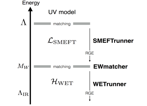
Given some initial conditions for the Warsaw basis at the high-energy scale , obtained from the matching of a UV model to the SMEFT, DsixTools allows the user to perform the full one-loop Renormalization Group Evolution (RGE) down to the electroweak scale. Furthermore, when the physics of interest lies well below the electroweak scale, it is useful to perform a matching of the dimension-six basis to a low-energy EFT in the broken electroweak phase. In the so-called Weak Effective Theory (WET), the SM heavy degrees of freedom (top quark, Higgs, and ) have been integrated out. DsixTools implements the tree-level matching of the Warsaw basis to and operators of the WET based on the results obtained in [17]. Last but not least, the relevant effects due to QCD and QED running from the electroweak scale down to the -quark mass scale in the WET is also implemented in DsixTools, using the results in [18].
DsixTools is structured into different modules, each of them taking care of a specific task. Their functionality is described in Sec. 2. Sec. 3 explains how to download and load DsixTools whereas a detailed review of DsixTools and its modules is given in Sec. 4. A summary is given in Sec. 5. Finally, this manual includes several appendices to document all the features present in DsixTools: A contains details of the conventions used for the implementation of the SMEFT, B contains the SMEFT RGEs, C describes relevant aspects of the WET, D contains a detailed description of the DsixTools routines, E is devoted to compile the SMEFT and WET parameters list and F gives results for the Baryon-number-violating operators in the fermion mass basis.
2 DsixTools in a nutshell
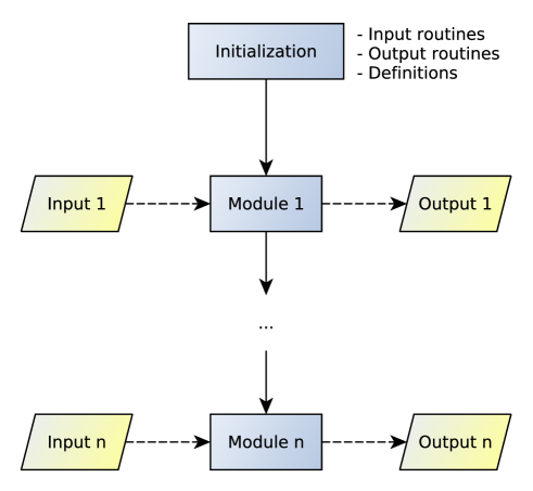
DsixTools is a modular package, with each module performing an independent task related to dimension-six effective operators. The different modules can be easily communicated with each other, since one module’s output can be used as input for another module. In practice, this means that a particular project with DsixTools can involve all modules or just a few, depending on the user’s goals. Fig. 1 shows the global flowchart of DsixTools.
The current version of DsixTools contains three independent modules, called: SMEFTrunner, EWmatcher and WETrunner. The SMEFTrunner module implements:
- •
-
•
The one-loop RGEs for the dimension-six operators in the Warsaw basis from Refs. [3, 4, 5].222We have taken into account the errata published in http://einstein.ucsd.edu/smeft/.
-
•
The one-loop RGEs for the dimension-six Baryon-number-violating operators using the results in [6].
The EWmatcher module implements:
-
•
The tree-level matching of the Warsaw basis to the and operators of the WET at the electroweak scale, using the results in [17].
The WETrunner module implements:
-
•
QCD and QED RGEs in the WET from the electroweak scale down to the low-energy scale . The WETrunner module fixes by default , the -quark mass scale, and uses the RGEs derived in [18].
3 Downloading and loading DsixTools
DsixTools is free software under the copyleft of the GNU General Public License. It can be downloaded from the web page [23]:
After placing the DsixTools folder in the Applications folder of the Mathematica base directory, the user can load DsixTools with the command
Alternatively, the user can place the DsixTools folder in a given directory and call the package by specifying its location via
before executing the Needs command. We also recommend to use
at the beginning of all projects with DsixTools.
4 Using DsixTools
In this Section we describe how to use DsixTools in detail. Once the package has been loaded, the user can already execute some basic I/O functions and routines. Several global variables are also introduced at this stage. Here we list the general DsixTools routines:
-
•
LoadModule[moduleName]: Loads the DsixTools module moduleName.
-
•
MyPrint[string]: Prints the message string. It can be switched on and off by using the DsixTools routines TurnOnMessages and TurnOffMessages.
-
•
TurnOnMessages: Turns on the messages written by DsixTools.
-
•
TurnOffMessages: Turns off the messages written by DsixTools.
-
•
ReadInputFiles[options_file, WCsInput_file, {SMInput_file}]: Reads all the input files. The third argument is optional and should be absent when the routine is used to read WET input.
-
•
WriteInputFiles[options_file, WCsInput_file, {SMInput_file},data]: Creates input files with the parameter values in data. The third argument is optional and should be absent when the routine is used to write WET input.
-
•
WriteAndReadInputFiles[options_file,WCsInput_file,{SMInput_file}]: Writes data into new input files and then reads them. The third argument is optional and should be absent when the routine is used to write and read WET input.
-
•
NewInput[parameter,newvalue,dispatch]: Replaces the current input (contained in the Mathematica dispatch dispatch) by a new one in which parameter takes the value newvalue.333For those not familiar with Mathematica dispatch tables, we clarify that these are optimized representations of lists of replacement rules. In practice they work in exactly the same way as replacement rules, but their execution time is much lower when the list of replacements is long.
-
•
NewScale[scale,newvalue]: Replaces the current value of scale by newvalue. Here scale can be either "high" or "low".
-
•
H[mat]: Returns the Hermitian conjugate of the matrix mat. If the option CPV has been set to 0 then it returns the transpose.
-
•
CC[x]: Returns the complex conjugate of x. If the option CPV is set to 0 then it returns x.
A more detailed description of these DsixTools routines can be found in D.1. Once DsixTools is loaded the user can already perform some basic operations. However, the real power of DsixTools resides in its modules. A project with DsixTools can involve one or many modules, depending on the user’s goals. For instance, if one is interested in the running of WET operators between the electroweak scale and the -quark mass scale, the WETrunner module suffices for the task. But if one wants to study the RGE evolution of the SMEFT operators and their matching to WET ones at the electroweak scale, both the SMEFTrunner and EWmatcher modules must be included in the project. In the following we proceed to describe the existing modules, the routines they include and how they can be combined together in a practical DsixTools project.
4.1 SMEFTrunner module
The SMEFTrunner module takes care of the one-loop RGE of the SMEFT between the high-energy scale and the electroweak scale. The module is based on the anomalous dimension matrices computed in [3, 4, 5] (for the Baryon-number-conserving operators) and [6] (for the Baryon-number-violating operators). This is the list of routines implemented in this module:
-
•
InitializeSMEFTrunnerInput: Initializes the input for the SMEFTrunner module.
-
•
FindParameterSMEFT[parameter]: Returns the position in which parameter is located within the Parameters list.
-
•
GetBeta: Computes the SMEFT functions.
-
•
LoadBetaFunctions: Constructs the SMEFT functions or reads them from a file.
-
•
RunRGEsSMEFT: Runs the SMEFT RGEs.
-
•
ExportSMEFTrunner: Exports the SMEFTrunner results to an output file.
-
•
WriteSMEFTrunnerOutputFile[Output_file,data]: Exports the SMEFTrunner results in data to Output_file.
More details about these routines can be found in D.2.
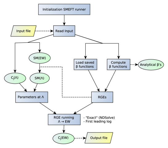
The general flowchart of the SMEFTrunner module can be seen in Fig. 3. The first step is to read the input. This not only includes the numerical values of the SMEFT WCs at the high-energy scale , but also the numerical values of the SM parameters and some options. The input and output format of DsixTools is inspired by the Supersymmetry Les Houches Accord (SLHA) [24, 25]. A complete options card would read:
For this particular example we have chosen the default options. In fact, if a flag is not present in the options file, its value will be taken as in this example. The user defines the high-energy and electroweak scales in the first block. We see that in this example the electroweak scale is fixed to GeV, the -boson mass, whereas the high-energy scale is TeV. Then the user defines several options. For instance, in this case CP-violation has been switched off by setting CPV to , but the user can also consider complex parameters setting CPV to . The comments accompanying the other options are self-explanatory, but we will review them below. A sample of a typical input card for the SM parameters is as follows:
Again, the input values are distributed in blocks, each devoted to a set of parameters. For instance, the SM gauge couplings are given in the block GAUGE. We note that the Yukawa matrices (and in general any complex parameter) are given in two blocks. For the up-quark Yukawas these are GU and IMGU: the first one is used for the real parts and the second for the imaginary ones. By default, the SM parameters are assumed to be given at the electroweak scale, where their experimental values are known. Then, before running down from to the electroweak scale they must be computed at . This is done by running up from the electroweak scale using pure SM RGEs, hence neglecting possible deviations caused by non-zero SMEFT WCs.444The user can check the validity of this approximation by using the SMEFTrunner routines, for instance by checking whether the resulting values for the SM parameters at the electroweak scale (after running down) do not match their initial values. This can be fixed by readjusting the SM parameters at . We note, however, that one should take into account NP corrections to the standard electroweak parameters induced by non-zero SMEFT WCs. However, in case the user prefers to give the SM parameters directly at high-energy scale , this can be done by setting the UseRGEsSM option to or, equivalently, by introducing a in flag number 5 of the options file,
This choice is recommended when the user wants to use the First leading log method to solve the RGEs, see below. Finally, a standard input card for the SMEFT WCs reads:
The notation for the operators is self-explanatory:
It is important to note that all WCs are assumed to vanish by default. Therefore, it suffices to include the non-zero WCs (and only these) in the input card. The rest can be absent.
In addition to getting input values at , the SMEFTrunner module constructs the SMEFT RGEs and prepares a routine for their evaluation. There are two ways to do this: (i) to “compute” the RGEs, or (ii) to read them from a file. In the first case, DsixTools takes their saved forms and computes all flavor traces and expands over all possible indices. In the second case, DsixTools simply reads them from a file (already present in the DsixTools folder). In both cases, the command to give this step is LoadBetaFunctions. The user can choose between these two methods in the options file using flag number . Method (i) is more time consuming but provides nice-looking functions in Mathematica format. This would be very useful for analytical studies. Moreover, the user can obtain these equations at any moment by using the routine GetBeta. Method (ii) is much faster and produces the RGEs in the format required for their immediate evaluation with the SMEFTrunner routines (in particular with RunRGEsSMEFT).
Once both the initial conditions (input values at ) and the RGEs are completely built, the user can apply the RGE to obtain the goal of SMEFTrunner: the SMEFT WCs at the electroweak scale. This is done with the RunRGEsSMEFT routine. We have implemented two different methods for the resolution of the RGEs:
-
•
“Exact”: This method applies the Mathematica internal command NDSolve for the numerical resolution of differential equations. Given the large number of differential equations involved in this case (several thousand), this might be time consuming, with each evaluation requiring a few (< 10) seconds, the exact number depending on the particular case and computer.
-
•
First leading log: This approximate method might be sufficient for many phenomenological studies, in particular when is not too far from the electroweak scale. The solution of the RGEs is obtained as
(4.1) where is any of the running parameters, is the renormalization scale and is the function for the evaluated at . This method is much faster but neglects subleading effects.
The user chooses between these two methods by setting the global option RGEsMethod to (for the NDSolve method) or (for the first leading log approximate method). This is also done via flag number 3 in the options card. After running, the results are saved in the array outSMEFTrunner as a function of . The ordering of the parameters is the same as in the Parameters global array, see E.555The position of a specific parameter can also be obtained by using the FindParameterSMEFT function, see D. Moreover, two important values of are predefined: tLOW () and tHIGH (). Therefore, for instance, one can obtain the value of the at the electroweak scale by evaluating
Finally, the output of SMEFTrunner can be exported to a text file. This is done by running ExportSMEFTrunner. The file Output_SMEFTrunner.dat is then generated, also with an SLHA format, completely analogous to the SMEFT WCs input card.
4.2 EWmatcher module
The EWmatcher module applies the tree-level matching of the Warsaw basis of the SMEFT to the and operators of the WET. For this purpose we make use of the analytical results obtained in [17]. This is the list of routines implemented in this module:
-
•
InitializeEWmatcherInput: Initializes the input for the EWmatcher module.
-
•
FindParameterWET[parameter]: Returns the position where parameter is located within the WETParameters list.
-
•
Biunitary[mat,dim]: Applies a biunitary transformation that diagonalizes the dim dim matrix mat.
-
•
RotateToMassBasis: Transforms the SMEFT WCs to the fermion mass basis.
-
•
ApplyEWmatching: Matches the SMEFT WCs onto the WET WCs.
-
•
Match[WC]: Returns the value of the WET Wilson coefficient WC after matching it to the SMEFT.
-
•
MatchAnalytical[WC]: Returns the analytical expression of the WET Wilson coefficient WC after matching it to the SMEFT.
-
•
WriteWCsMassBasisOutputFile[Output_file]: Exports the SMEFT 2- and 4-fermion WCs in the fermion mass basis to Output_file.
-
•
ExportEWmatcher: exports the EWmatcher results to an output file.
-
•
WriteEWmatcherOutputFile[Output_file,data]: Exports the EWmatcher results in data to Output_file.
Appendix D.3 contains more details about these routines
and functions.
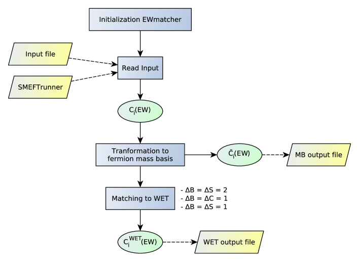
The EWmatcher module flowchart can be seen in Fig. 4. The first step is, as usual, to determine the input of the module. If the SMEFTrunner module has preceded the EWmatcher, the input is automatically created using the output of the former. Otherwise, the user can also provide an input file and start the DsixTools project with the EWmatcher module as first step.
In what concerns the input card, the same WCsInput.dat file that is read by the SMEFTrunner module can also be used as WCs input for the EWmatcher module. Instead of interpreting the input values as given at , the EWmatcher module will interpret them as given at .
Next, the EWmatcher transforms the SMEFT WCs to the fermion mass
basis, applying the required biunitary transformations to the fermion
mass matrices.666In the current version of DsixTools, the
dimension five Weinberg operator is absent and neutrinos remain
massless. For this reason, we have not considered rotations in the
lepton sector, which is assumed to be diagonal. This necessary step
is done by means of the RotateToMassBasis routine and gives, as
a result, the SMEFT WCs in the fermion mass basis, generally denoted
as .777The Baryon-number-conserving
coefficients in the mass basis were computed in
[17] whereas the Baryon-number-violating ones can be found
in F. In case the user is particularly interested in
these coefficients, they can be exported to an external text file by
running
Furthermore, RotateToMassBasis also creates the replacements array ToMassBasis, which can be used to print the numerical values of the
SMEFT WCs in the fermion mass basis. For example,
would print the numerical value of the coefficient .
The next step is the matching to the WET operators. For this the user
must execute
This creates the arrays BS2, BC1, BS1Hunprimed, BS1Hprimed, BS1GB, BS1SLunprimed and BS1SLprimed, containing the numerical values of the WET WCs at the electroweak scale. While BS2 and BC1 contain the results for the and coefficients, respectively, the other arrays contain the results for the ones, split into several sub-arrays with hadronic (H), semileptonic (SL) and magnetic, or gauge boson (GB) involving, WCs. They can also be accessed individually thanks to the function Match. For example, CBS1[e][1] // Match would print the numerical value of . If one is interested in the analytical expression after matching the function to use is MatchAnalytical, which only replaces the energy scales and the SM parameters by their numerical values.
Finally, the output of EWmatcher can be exported to a text file. This is done by running ExportEWmatcher, which generates the file Output_EWmatcher.dat with a compilation of all results obtained with this module.
4.3 WETrunner module
The WETrunner module is devoted to the RGE of the WET WCs between the electroweak scale and the infrared scale . In the current version of DsixTools, is set by default at -quark mass scale, GeV, and the RGE is based on the analytical results obtained in Ref. [18]. This is the list of routines implemented in this module:
-
•
InitializeWETrunnerInput: Initializes the input for the WETrunner module.
-
•
RunRGEsWET: Runs the WET RGEs.
-
•
ExportWETrunner: Exports the WETrunner results to an output file.
-
•
WriteWETrunnerOutputFile[Output_file,data,scale]: Exports the WETrunner results in data to Output_file after evaluating them at scale.
For more details about these routines see Appendix D.4.
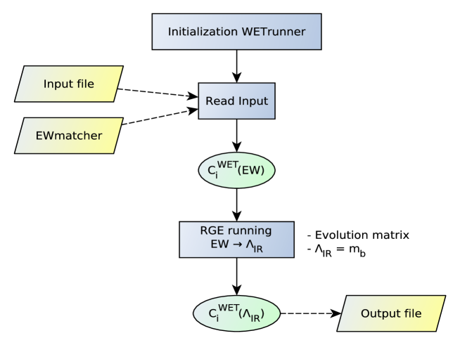
The general flowchart of the WETrunner module can be seen in Fig. 5. As for the EWmatcher module, the input for the WETrunner can be obtained directly (and automatically) from the previous module (EWmatcher in this case) if this is run before. Otherwise, the user can also provide new input values and begin a DsixTools project in this step of the chain. In this case, the input card for the WET WCs, which we will call WCsInput.dat as for the SMEFT ones, also follows a simple SLHA-inspired format:
We see that the first block gives the input value for the electroweak scale while the other blocks give the input values for the WET WCs. In this particular example the only non-vanishing WET WC is . It is important to note, however, that DsixTools must know that the input WCs are of WET type. This is done via the option inputWCsType, which must be set to (the default value is , which indicates SMEFT WCs) before reading the input file with the ReadInputFiles routine. This option choice can also be achieved by using the flag number in the options card:
Once the input has been read (or taken from the EWmatcher module) one
can proceed to the RGE of the WET WCs. The WETrunner module
implements an evolution matrix formalism for this step, based on the
results of Ref. [18]. This can be performed with the RunRGEsWET
which creates the numerical arrays BS2Low, BC1Low, BS1unprimedLow and BS1primedLow, all of them functions of . Therefore, in order to find the values of the WET
WCs at the -quark mass scale one can evaluate commands like
where mb is the global DsixTools variable containing the -quark mass (in GeV). This command would print the numerical value of . Finally, the results can be exported to an output file with the routine ExportWETrunner. This creates the text file Output_WETrunner.dat with the values of all WET WCs at the infrared scale.
5 Summary
We have presented DsixTools, a Mathematica package for the handling of the dimension-six SMEFT and WET. DsixTools facilitates the treatment of these two effective theories in a systematic and complete manner.
DsixTools is a modular code. In the current version, it includes three independent modules, designed for specific tasks related to the SMEFT and WET. The SMEFTrunner performs the one-loop RGE from the UV scale to the electroweak scale, the EWmatcher matches the SMEFT Wilson coefficients to the and operators of the WET, and the WETrunner runs these down to an IR scale, in this case the -quark mass scale.
The structure of DsixTools allows for an easy implementation of new modules. Therefore, the current content of the package is expected to grow substantially with future improvements, including additional tools and features. The final outcome of this endevour will be a complete and powerful framework for the systematic exploration of new physics models using the language of Effective Field Theories.
Acknowledgements
We thank Aneesh Manohar for comments on the manuscript. The work of A.C. is supported by the Alexander von Humboldt Foundation. The work of J.F. is supported in part by the Spanish Government, by Generalitat Valenciana and by ERDF funds from the EU Commission [grants FPA2011-23778,FPA2014-53631-C2-1-P, PROMETEOII/2013/007, SEV-2014-0398]. J.F. also acknowledges VLC-CAMPUS for an “Atracció de Talent” scholarship. A.V. acknowledges financial support from the “Juan de la Cierva” program (27-13-463B-731) funded by the Spanish MINECO as well as from the Spanish grants FPA2014-58183-P, Multidark CSD2009-00064, SEV-2014-0398 and PROMETEOII/ 2014/084 (Generalitat Valenciana). J.V. is funded by the Swiss National Science Foundation and acknowledges support from Explora project FPA2014-61478-EXP. A.C. thanks the Albert Einstein Center for Fundamental Physics of the University of Bern for their hospitality and support while part of this work was performed.
Appendix A Standard Model Effective Field Theory
The Lagrangian for the SMEFT can be written as
| (A.1) |
Here is the new physics scale suppressing higher dimensional operators, assumed to be much larger than the electroweak scale. There is only one operator of dimension five, the so-called Weinberg operator that gives a Majorana mass term for the neutrinos [26]. A non-redundant basis of dimension-six operators was introduced in [2] and is known as the Warsaw basis. We list these operators in Tables 2, 3 and 4. Barring flavor structure, and assuming Baryon number conservation, there are 59 operators, some of which are non-Hermitian, yielding in total 76 real coefficients. Taking into account flavour indices, the dimension-six Lagrangian contains 1350 CP-even and 1149 CP-odd operators, for a total of 2499 hermitian operators [5]. Finally, the complete set of independent dimension-6 Baryon number violating operators were identified in [27]. Barring flavor structure, there are only 4 Baryon-number-violating operators. These are listed in Table 5.
The implementation of the SMEFT in DsixTools follows the conventions used in [2].888The reader should keep in mind that these conventions differ from those used in [3, 4, 5]. The differences appear in the normalization of and , the definition of the Yukawa matrices, the name of the gauge couplings, and in whether the NP scale is introduced into the definition of the WCs. The SM renormalizable Lagrangian is given by
| (A.2) |
Here and denote gauge indices associated to and . The fields and correspond to the lepton and quark doublets of the SM, while are the right-handed fields. The Higgs doublet is denoted by . The Yukawa couplings are matrices in flavor space. The covariant derivative is generically defined as
| (A.3) |
where and are, respectively, the , and gauge couplings and gauge fields. and are the corresponding gauge group generators. The hypercharge assignments for the matter fields are given in Table 1.
| Field | ||||||
|---|---|---|---|---|---|---|
DsixTools also implements the running of the terms
| (A.4) |
calculated in [3]. The dual tensors are defined as (with ).
| Baryon-number-violating | |
|---|---|
Appendix B SMEFT Renormalization Group Equations
At leading order, the RGEs governing the energy evolution of the SMEFT Wilson coefficients can be written as
| (B.1) |
Here is the renormalization scale, is the anomalous dimensions matrix and are the functions. The complete anomalous dimension matrix for the dimension-six SMEFT operators has been recently computed in [3, 4, 5, 6]. We collect here the resulting functions, adapted to our notation and conventions.
First, we give some definitions that turn out to be useful in order to simplify the functions:
| (B.2) | ||||
| (B.3) | ||||
| (B.4) | ||||
| (B.5) | ||||
| (B.6) |
as well as
| (B.7) |
and the wavefunction renormalization terms
| (B.8) |
and
| (B.9) | ||||
| (B.10) | ||||
| (B.11) | ||||
| (B.12) | ||||
| (B.13) |
Finally we also use the following definitions
| (B.14) | ||||
| (B.15) | ||||
| (B.16) |
| (B.17) | ||||
| (B.18) | ||||
| (B.19) | ||||
| (B.20) |
| (B.21) |
| (B.22) | ||||
| (B.23) |
| (B.24) | ||||
| (B.25) | ||||
| (B.26) | ||||
| (B.27) | ||||
| (B.28) | ||||
| (B.29) | ||||
| (B.30) | ||||
| (B.31) |
| (B.32) | ||||
| (B.33) | ||||
| (B.34) |
| (B.35) | ||||
| (B.36) | ||||
| (B.37) | ||||
| (B.38) | ||||
| (B.39) | ||||
| (B.40) | ||||
| (B.41) | ||||
| (B.42) |
| (B.43) | ||||
| (B.44) | ||||
| (B.45) | ||||
| (B.46) | ||||
| (B.47) | ||||
| (B.48) | ||||
| (B.49) | ||||
| (B.50) |
| (B.51) | ||||
| (B.52) | ||||
| (B.53) | ||||
| (B.54) | ||||
| (B.55) |
| (B.56) | ||||
| (B.57) | ||||
| (B.58) | ||||
| (B.59) | ||||
| (B.60) | ||||
| (B.61) | ||||
| (B.62) | ||||
| (B.63) | ||||
| (B.64) | ||||
| (B.65) | ||||
| (B.66) | ||||
| (B.67) | ||||
| (B.68) | ||||
| (B.69) | ||||
| (B.70) |
| (B.71) |
| (B.72) | ||||
| (B.73) | ||||
| (B.74) | ||||
| ç | ||||
| (B.75) |
| (B.76) | ||||
| (B.77) | ||||
| (B.78) | ||||
| (B.79) |
The RGEs for the SM parameters get also modified in the presence of the dim-6 operators. Using an analogous notation for their functions
| (B.80) |
these are given by
| (B.81) | ||||
| (B.82) | ||||
| (B.83) | ||||
| (B.84) | ||||
| (B.85) | ||||
| (B.86) | ||||
| (B.87) | ||||
| (B.88) |
In the absence of contributions from the dim-6 operators one recovers the well-known SM RGEs [19, 20, 21, 22]. Notice however that we do not include an normalization factor for , and hence the usual expressions are found by replacing . Finally, we also have in the SM Lagrangian
| (B.89) |
with
| (B.90) |
Appendix C Weak Effective Theory for physics
The Hamiltonian for the WET can be written as
| (C.1) |
where is the usual QCD and QED Lagrangian for the light fermions, contains pure-SM dimension-six operators and the coefficients contain all beyond the Standard Model effects. The sum over the index runs over all operators defined below.999At the moment DsixTools only includes a limited subset of WET operators: , and operators. See Ref. [18] for definitions and conventions.
C.1 operators
In the case of operators, the basis is given by
| (C.2) |
where we denote with primed indices the operators with opposite chirality. and are indices.
C.2 operators
The basis for the operators is given by
| (C.3) | ||||||||
with .
C.3 operators
There are three classes of operators: Magnetic, hadronic (4-quark) and semileptonic operators. These are chosen as:
-
•
Magnetic penguins:
| (C.4) |
() are the generators.
-
•
Hadronic ():
| (C.5) | ||||||
where . In the case of , the color-octet operators are Fierz-equivalent to the color-singlet ones and are not included in the basis. In addition, the analogous set with opposite chirality is needed:
| (C.6) |
-
•
Hadronic ():
| (C.7) |
Again, the color-octet operators are Fierz-redundant and have been ommited.
-
•
Semileptonic:
| (C.8) |
with .
Appendix D DsixTools routines
In this Appendix we list the public routines implemented in DsixTools. The user can take advantage of them when writing a project with DsixTools.
D.1 General DsixTools routines
LoadModule[moduleName]
Loads the DsixTools module moduleName. Once this command is
evaluated, the module is initialized and all its routines are
available to the user.
Requires: Nothing. This routine can be used as soon as
DsixTools is loaded.
Arguments: In the current version of DsixTools, moduleName can either be "SMEFTrunner", "EWmatcher" or "WETrunner".
Example: LoadModule["SMEFTrunner"] loads the SMEFTrunner module.
MyPrint[string]
Prints the message string. It can be switched on and off by using
the DsixTools routines TurnOnMessages and TurnOffMessages.
Requires: Nothing. This routine can be used as soon as
DsixTools is loaded.
Arguments: string must be a valid Mathematica string.
Example: MyPrint["I am using DsixTools"] prints a simple message.
TurnOnMessages
Turns on the messages written by the DsixTools routines.
Requires: Nothing. This routine can be used as soon as DsixTools is loaded.
TurnOffMessages
Turns off the messages written by the DsixTools routines. The only
exception are the messages written when a new module is loaded, which
cannot be switched off.
Requires: Nothing. This routine can be used as soon as DsixTools is loaded.
ReadInputFiles[options_file,WCsInput_file,{SMInput_file}]
Reads all input files.
Requires: Nothing. This routine can be used as soon as
DsixTools is loaded.
Arguments: options_file and WCsInput_file
are the paths to the options and WCs input files. WCsInput_file
can contain either SMEFT or WET WCs. The SMInput_file argument
is the path to the input card with the values of the SM parameters and
is optional: it should be absent when this routine is used to read WET
input.
Example: ReadInputFiles["Options.dat","WCsInput.dat","SMInput.dat"] reads the content of three SMEFT input files. ReadInputFiles["Options.dat","WCsInput.dat"] reads the content of two WET input files.
WriteInputFiles[options_file,WCsInput_file,{SMInput_file},data]
Creates input files with the parameter values in data. This
routine can be used to export the input values defined by the user in
a project to external text files, later to be read by DsixTools.
Requires: Nothing. This routine can be used as soon as
DsixTools is loaded.
Arguments: options_file and WCsInput_file
are the paths to the options and WCs input files created by this
routine. data is an array where the input values have a precise
ordering, defined by the ordering in the Parameters (for SMEFT
input) and WETParameters (for WET input) global arrays, see
E. The SMInput_file argument is the path to
the input card with the values of the SM parameters and is optional:
it should be absent when this routine is used to write WET input.
Example: WriteInputFiles["Options.dat","WCsInput.dat","SMInput.dat", data] exports the SMEFT values in data to three input files. WriteInputFiles["Options.dat", "WCsInput.dat", data] exports the WET values in data to two input files. These input files can later be read by DsixTools.
WriteAndReadInputFiles[options_file,WCsInput_file,{SMInput_file}]
Writes data into new input files and then reads them. In essence,
running this routine is equivalent to running WriteInputFiles
and ReadInputFiles.
Requires: Before using the routine the data to be exported
(and later read) must be declared. In case of SMEFT input, all SM
parameters must be set to their input values by giving values to
variables of the form Init[SM_parameter] and all WC values will
be assumed to vanish unless they are declared in a similar way. In
case of WET input, only the WC values must be declared. Finally, the
options will be assumed to take default values unless set to other
choices.
Arguments: options_file and WCsInput_file
are the paths to the options and WCs input files created by this
routine. The SMInput_file argument is the path to the input
card with the values of the SM parameters and is optional: it should
be absent when this routine is used to write and read WET input.
Example: WriteAndReadInputFiles["Options.dat","WCsInput.dat","SMInput.dat"] exports the previously declared
values to three SMEFT input files and then reads them.
WriteAndReadInputFiles["Options.dat", "WCsInput.dat"] exports the
previously declared values to two WET input files and then reads them.
NewInput[parameter,newvalue,dispatch]
Replaces the current input (contained in the Mathematica dispatch dispatch) by a new one in which parameter takes the value
newvalue. This routine is particularly useful for projects
involving loops with varying parameters.
Requires: Input values must have been introduced before
using this routine, for instance using the ReadInputFiles
routine. Only in this way the dispatch dispatch would have been
defined.
Arguments: parameter must be a valid name for a
DsixTools parameter. These can be found in the global arrays Parameters (in case of SMEFT input) and WETparameters (in
case of WET input), see E. newvalue must be a
valid number (in general complex). dispatch is the name of the
Mathematica dispatch where the input values are saved. By default, this is
input. In the SMEFTrunner module there is also the
internal dispatch inputSMEFTrunner.
Example: NewInput[LL[1,1,1,2],1.0,input] changes the input value (at the high-energy scale ) of to .
NewScale[scale,newvalue]
Replaces the current value of scale by newvalue. This
routine is particularly useful for projects involving loops with
varying energy scales.
Requires: Nothing. This routine can be used as soon as
DsixTools is loaded.
Arguments: scale can be either "high" or "low". newvalue must be a valid positive real number. As with
other dimensionful parameters, the scale should be given in GeV.
Example: NewScale["high",1000] changes the high energy scale to TeV.
H[mat]
Returns the Hermitian conjugate of the matrix mat. If the option CPV has been set to 0 then it returns the transpose.
Requires: The global variable CPV must have been set
to either 0 (for real parameters) or 1 (for complex
parameters) before using this function.
Arguments: mat must be a valid matrix.
Example: H[Gu] returns the Hermitian conjugate of the up-quarks Yukawa matrix .
CC[x]
Returns the complex conjugate of x. If the option CPV has been set to 0 then it returns x.
Requires: The global variable CPV must have been set
to either 0 (for real parameters) or 1 (for complex
parameters) before using this function.
Arguments: x must be a valid complex number.
Example: CC[GU[1,2]/.input] returns if CPV has been set to 1 and if CPV has been set to 0, using for its input value.
D.2 SMEFTrunner routines
InitializeSMEFTrunnerInput
Initializes the input for the SMEFTrunner module. This initialization creates the
dispatches inputSMEFTrunner and inputSMEFTrunnerSM. The
user does not need to use this routine, as it is automatically
executed when the SMEFTrunner module is loaded.
Requires: The SMEFTrunner module must have been loaded in order to use this routine.
FindParameterSMEFT[parameter]
Returns the position of parameter in the Parameters
list. If one uses a generic element name as argument, FindParameterSMEFT will return a list with all positions where it
appears in Parameters.
Requires: Nothing. This routine can be used as soon as
DsixTools is loaded.
Arguments: parameter can be either the name of a SM
parameter or SMEFT WC, or the generic name of an element of one of the
2- or 4-fermion parameters.
Example: FindParameterSMEFT[LQ3[2, 2, 2, 3]] returns {355}, the position of in the Parameters list. FindParameterSMEFT[LQ3] returns {327, 328, …, 371}, since the WCs are saved in these positions of the Parameters list.
GetBeta
Computes the SMEFT functions analytically. After running this
routine they can be read by evaluating quantities of the form [parameter]. For instance, the
functions can be obtained by evaluating [lq1]. Table
LABEL:tab:SMEFTparameters contains the names used for all SMEFT
functions.
Requires: The SMEFTrunner module must have been loaded in order to use this routine. Moreover, the global variable CPV must have been set to either 0 (for real parameters) or 1 (for complex parameters) before using this function.
LoadBetaFunctions
Constructs the SMEFT functions (using GetBeta
internally) or reads them from a file.
Requires: The SMEFTrunner module must have been loaded and the option ReadRGEs set in order to use this routine.
RunRGEsSMEFT
Runs the SMEFT RGEs.
Requires: The SMEFTrunner module must have been loaded and the option RGEsMethod set in order to use this routine.
ExportSMEFTrunner
Exports the SMEFTrunner results to the output file Output_SMEFTrunner.dat.
Requires: The SMEFTrunner module must have been loaded and the option exportSMEFTrunner set in order to use this routine.
WriteSMEFTrunnerOutputFile[Output_file,data]
Exports the SMEFTrunner results in data to Output_file.
Requires: The SMEFTrunner module must have been loaded in
order to use this routine.
Arguments: Output_file is the path to the
SMEFTrunner output file. data is an array containing the
results obtained with SMEFTrunner. It must contain the same of
elements and ordered in exactly the same way as outSMEFTrunner.
Example:
WriteSMEFTrunnerOutputFile["Output_SMEFTrunner.dat",outSMEFTrunner/.t->tLOW]
exports the data saved in the outSMEFTrunner array, evaluated at
, into the text file Output_SMEFTrunner.dat.
D.3 EWmatcher routines
InitializeEWmatcherInput
Initializes the input for the EWmatcher module. The user does not
need to use this routine, as it is automatically executed when the
EWmatcher module is loaded.
Requires: The EWmatcher module must have been loaded in order to use this routine.
FindParameterWET[parameter]
Returns the position of parameter in the WETParameters
list. If one uses a generic element name as argument, FindParameterWET will return a list with all positions where it
appears in WETParameters.
Requires: Nothing. This routine can be used as soon as
DsixTools is loaded.
Arguments: parameter must be the name of a WET WC.
Example: FindParameterWET[CBS1[][1]] returns {71}, the position of within the WETParameters list. FindParameterWET[CBS1[]] returns {71, 72, 73, 74, 75}, since the WCs are saved in these positions of the WETParameters list.
RotateToMassBasis
Transforms the SMEFT WCs to the fermion mass basis. It also creates
the replacements array ToMassBasis, which can be used to print
the numerical values of the SMEFT WCs in the fermion mass basis.
Requires: The EWmatcher module must have been loaded in order to use this routine.
Biunitary[mat,dim]
Applies a biunitary transformation that diagonalizes the dim dim
matrix mat. It returns three outputs: the square root of the
eigenvalues of mat† mat (or, equivalently, mat mat†) and the unitary matrices and
that diagonalize mat as mat mat.
Requires: The EWmatcher module must have been loaded in order to use this function.
Arguments: mat must be a valid dim
dim matrix.
Example: Biunitary[Gu/.input,3] returns the square root of the eigenvalues of (or, equivalently, ), as well as the matrices and that diagonalize as . Here is the input value for the up-quarks Yukawa matrix.
ApplyEWmatching
Matches the SMEFT WCs onto the WET WCs. After using this routine
several arrays containing the numerical values of the WET WCs at the
electroweak scale are created. The result of this step can also be accessed by using the Match and MatchAnalytical functions.
Requires: The EWmatcher module must have been loaded in order to use this function.
Match[WC]
Returns the value of the WET Wilson coefficient WC after matching it to the SMEFT.
Requires: The EWmatcher module must have been loaded in order to use this function. Furthermore, the ApplyEWmatching routines must have been run before using this function.
Arguments: WC must be the name of a valid SMEFT WC.
Example: Match[CBS1[d][1]] prints the numerical value of the WC.
MatchAnalytical[WC]
Returns the analytical expression of the WET Wilson coefficient WC after matching it to the SMEFT. Only the energy scales and the SM parameters are replaced by numerical values in this function.
Requires: The EWmatcher module must have been loaded in order to use this function. Furthermore, the ApplyEWmatching routines must have been run before using this function.
Arguments: WC must be the name of a valid SMEFT WC.
Example: Match[CBS1[d][1]] prints the analytical expression of the WC.
WriteWCsMassBasisOutputFile[Output_file]
Exports the SMEFT 2- and 4-fermion WCs in the fermion mass basis to Output_file.
Requires: The EWmatcher module must have been loaded in order to use this function. Furthermore, the ApplyEWmatching routines must have been run before using this function.
Arguments: Output_file is the path to the text file
where the SMEFT WCs in the fermion mass basis will be exported.
Example: WriteWCsMassBasisOutputFile["Output_WCsMassBasis.dat"] will export the SMEFT WCs in the fermion mass basis to the file "Output_WCsMassBasis.dat".
ExportEWmatcher
Exports the EWmatcher results to the output file Output_EWmatcher.dat.
Requires: The EWmatcher module must have been loaded and the option exportEWmatcher set in order to use this routine.
WriteEWmatcherOutputFile[Output_file,data]
Exports the EWmatcher results in data to Output_file.
Requires: The EWmatcher module must have been loaded in
order to use this routine.
Arguments: Output_file is the path to the
EWmatcher output file. data is an array containing the results
obtained with EWmatcher. The precise ordering of the WET WCs in data is given by that in WETParameters, see
E.
Example: WriteEWmatcherOutputFile["Output_EWmatcher.dat",dataOutput] exports the data saved in the dataOutput array to the Output_EWmatcher.dat text file.
D.4 WETrunner routines
InitializeWETrunnerInput
Initializes the input for the WETrunner module. The user does not
need to use this routine, as it is automatically executed when the
WETrunner module is loaded.
Requires: The WETrunner module must have been loaded in order to use this routine.
RunRGEsWET
Runs the WET RGEs.
Requires: The WETrunner module must have been loaded in order to use this routine.
ExportWETrunner
Exports the WETrunner results to the output file Output_WETrunner.dat.
Requires: The WETrunner module must have been loaded and the option exportWETrunner set in order to use this routine.
WriteWETrunnerOutputFile[Output_file,data,scale]
Exports the WETrunner results in data to Output_file after evaluating them at scale.
Requires: The WETrunner module must have been loaded in
order to use this routine.
Arguments: Output_file is the path to the
WETrunner output file. data is an array containing the results
obtained with WETrunner. The precise ordering of the WET WCs in data is given by BS2Low-BC1Low-BS1unprimedLow-BS1primedLow, following exactly the ordering
in WETParameters (see E), and they must be
evaluated at scale.
Example:
WriteWETrunnerOutputFile["Output_WETrunner.dat",dataOutput,mb]
will export the data saved in the dataOutput array, evaluated at
, into the Output_WETrunner.dat text file.
Appendix E DsixTools parameters
In this Appendix we provide additional details about the SMEFT and WET parameters used in DsixTools. These can be useful to properly read or write some variables in a Mathematica session using DsixTools.
E.1 SMEFT parameters
Table LABEL:tab:SMEFTparameters provides a complete list of the SMEFT parameters used in DsixTools. In addition to the SMEFT WCs, this includes the SM parameters (gauge couplings, Yukawa matrices and scalar and parameters). This table is particularly useful to identify the names given to the elements of 2- and 4-fermion WCs, as well as the functions used in the SMEFTrunner module.
| Position | Parameter(s) | DsixTools name | Elements | function | Type | Category |
| 1 | g | - | [g] | 0F | 0 | |
| 2 | gp | - | [gp] | 0F | 0 | |
| 3 | gs | - | [gs] | 0F | 0 | |
| 4 | - | [] | 0F | 0 | ||
| 5 | [GeV2] | m2 | - | [m2] | 0F | 0 |
| 6-14 | Gu | GU[i,j] | [GuX] | 2F | 1 | |
| 15-23 | Gd | GD[i,j] | [GdX] | 2F | 1 | |
| 24-32 | Ge | GE[i,j] | [GeX] | 2F | 1 | |
| 33 | - | [] | 0F | 0 | ||
| 34 | p | - | [p] | 0F | 0 | |
| 35 | s | - | [s] | 0F | 0 | |
| 36 | G | - | [G] | 0F | 0 | |
| 37 | Gtilde | - | [Gtilde] | 0F | 0 | |
| 38 | W | - | [W] | 0F | 0 | |
| 39 | Wtilde | - | [Wtilde] | 0F | 0 | |
| 40 | - | [] | 0F | 0 | ||
| 41 | - | [] | 0F | 0 | ||
| 42 | DD | - | [D] | 0F | 0 | |
| 43 | G | - | [G] | 0F | 0 | |
| 44 | B | - | [B] | 0F | 0 | |
| 45 | W | - | [W] | 0F | 0 | |
| 46 | WB | - | [WB] | 0F | 0 | |
| 47 | Gtilde | - | [Gtilde] | 0F | 0 | |
| 48 | Btilde | - | [Btilde] | 0F | 0 | |
| 49 | Wtilde | - | [Wtilde] | 0F | 0 | |
| 50 | WtildeB | - | [WtildeB] | 0F | 0 | |
| 51-59 | WC[u] | U[i,j] | [u] | 2F | 1 | |
| 60-68 | WC[d] | D[i,j] | [d] | 2F | 1 | |
| 69-77 | WC[e] | E[i,j] | [e] | 2F | 1 | |
| 78-86 | WC[eW] | EW[i,j] | [eW] | 2F | 1 | |
| 87-95 | WC[eB] | EB[i,j] | [eB] | 2F | 1 | |
| 96-104 | WC[uG] | UG[i,j] | [uG] | 2F | 1 | |
| 105-113 | WC[uW] | UW[i,j] | [uW] | 2F | 1 | |
| 114-122 | WC[uB] | UB[i,j] | [uB] | 2F | 1 | |
| 123-131 | WC[dG] | DG[i,j] | [dG] | 2F | 1 | |
| 132-140 | WC[dW] | DW[i,j] | [dW] | 2F | 1 | |
| 141-149 | WC[dB] | DB[i,j] | [dB] | 2F | 1 | |
| 150-155 | WC[l1] | L1[i,j] | [l1] | 2F | 2 | |
| 156-161 | WC[l3] | L3[i,j] | [l3] | 2F | 2 | |
| 162-167 | WC[e] | E[i,j] | [e] | 2F | 2 | |
| 168-173 | WC[q1] | Q1[i,j] | [q1] | 2F | 2 | |
| 174-179 | WC[q3] | Q3[i,j] | [q3] | 2F | 2 | |
| 180-185 | WC[u] | U[i,j] | [u] | 2F | 2 | |
| 186-191 | WC[d] | D[i,j] | [d] | 2F | 2 | |
| 192-200 | WC[ud] | UD[i,j] | [ud] | 2F | 1 | |
| 201-227 | WC[ll] | LL[i,j,k,l] | [ll] | 4F | 4 | |
| 228-254 | WC[qq1] | QQ1[i,j,k,l] | [qq1] | 4F | 4 | |
| 255-281 | WC[qq3] | QQ3[i,j,k,l] | [qq3] | 4F | 4 | |
| 282-326 | WC[lq1] | LQ1[i,j,k,l] | [lq1] | 4F | 5 | |
| 327-371 | WC[lq3] | LQ3[i,j,k,l] | [lq3] | 4F | 5 | |
| 372-392 | WC[ee] | EE[i,j,k,l] | [ee] | 4F | 6 | |
| 393-419 | WC[uu] | UU[i,j,k,l] | [uu] | 4F | 4 | |
| 420-446 | WC[dd] | DD[i,j,k,l] | [dd] | 4F | 4 | |
| 447-491 | WC[eu] | EU[i,j,k,l] | [eu] | 4F | 5 | |
| 492-536 | WC[ed] | ED[i,j,k,l] | [ed] | 4F | 5 | |
| 537-581 | WC[ud1] | UD1[i,j,k,l] | [ud1] | 4F | 5 | |
| 582-626 | WC[ud8] | UD8[i,j,k,l] | [ud8] | 4F | 5 | |
| 627-671 | WC[le] | LE[i,j,k,l] | [le] | 4F | 5 | |
| 672-716 | WC[lu] | LU[i,j,k,l] | [lu] | 4F | 5 | |
| 717-761 | WC[ld] | LD[i,j,k,l] | [ld] | 4F | 5 | |
| 762-806 | WC[qe] | QE[i,j,k,l] | [qe] | 4F | 5 | |
| 807-851 | WC[qu1] | QU1[i,j,k,l] | [qu1] | 4F | 5 | |
| 852-896 | WC[qu8] | QU8[i,j,k,l] | [qu8] | 4F | 5 | |
| 897-941 | WC[qd1] | QD1[i,j,k,l] | [qd1] | 4F | 5 | |
| 942-986 | WC[qd8] | QD8[i,j,k,l] | [qd8] | 4F | 5 | |
| 987-1067 | WC[ledq] | LEDQ[i,j,k,l] | [ledq] | 4F | 3 | |
| 1068-1148 | WC[quqd1] | QUQD1[i,j,k,l] | [quqd1] | 4F | 3 | |
| 1149-1229 | WC[quqd8] | QUQD8[i,j,k,l] | [quqd8] | 4F | 3 | |
| 1230-1310 | WC[lequ1] | LEQU1[i,j,k,l] | [lequ1] | 4F | 3 | |
| 1311-1391 | WC[lequ3] | LEQU3[i,j,k,l] | [lequ3] | 4F | 3 | |
| 1392-1472 | WC[duql] | DUQL[i,j,k,l] | [duql] | 4F | 3 | |
| 1473-1526 | WC[qque] | QQUE[i,j,k,l] | [qque] | 4F | 7 | |
| 1527-1583 | WC[qqql] | QQQL[i,j,k,l] | [qqql] | 4F | 8 | |
| 1584-1664 | WC[duue] | DUUE[i,j,k,l] | [duue] | 4F | 3 |
It is well known that some of the 2- and 4-fermion operators in the SMEFT posess specific symmetries under the exchange of flavor indices. This translates into an index symmetry for the corresponding WCs. For instance, the Wilson coefficient is a Hermitian matrix, hence following the symmetry relation . More complicated index symmetries exist for some of the 4-fermion WCs. In all these cases, the number of independent WCs gets reduced. For example, the 4-fermion WC does not contain () independent complex WCs, but just real and imaginary independent components. Therefore, it is convenient to restrict the number of parameters considered in SMEFT calculations to just the independent ones. In DsixTools we have followed this approach, dropping redudant WCs in all calculations. This is what motivates the introduction of an index symmetry category column in Table LABEL:tab:SMEFTparameters. The meaning of the different categories is given by:
| Category | Meaning |
|---|---|
| 0 | 0F scalar object |
| 1 | 2F general matrix |
| 2 | 2F Hermitian matrix |
| 3 | 4F general object |
| 4 | 4F two identical currents |
| 5 | 4F two independent currents |
| 6 | 4F two identical currents - special case |
| 7 | 4F Baryon-number-violating - special case |
| 8 | 4F Baryon-number-violating - special case |
We see that, apart from the WCs in categories 0, 1 and 3, all other WCs have index symmetries. Furthermore, there are three WCs with special symmetries, not shared by any other WC: , and . In Table LABEL:tab:SMEFTnonredundant we list the independent WCs contained in each category. This, combined with Table LABEL:tab:SMEFTparameters, completely allows the user to determine the position of a given parameter in the Parameters array. In any case, we remind the reader that the function FindParametersSMEFT can also be used for this purpose.
| 1 | 2 | 3 | 4 | 5 | 6 | 7 | 8 | |
| 1 | {1, 1} | {1, 1} | {1, 1, 1, 1} | {1, 1, 1, 1} | {1, 1, 1, 1} | {1, 1, 1, 1} | {1, 1, 1, 1} | {1, 1, 1, 1} |
| 2 | {1, 2} | {1, 2} | {1, 1, 1, 2} | {1, 1, 1, 2} | {1, 1, 1, 2} | {1, 1, 1, 2} | {1, 1, 1, 2} | {1, 1, 1, 2} |
| 3 | {1, 3} | {1, 3} | {1, 1, 1, 3} | {1, 1, 1, 3} | {1, 1, 1, 3} | {1, 1, 1, 3} | {1, 1, 1, 3} | {1, 1, 1, 3} |
| 4 | {2, 1} | {2, 2} | {1, 1, 2, 1} | {1, 1, 2, 2} | {1, 1, 2, 2} | {1, 1, 2, 2} | {1, 1, 2, 1} | {1, 1, 2, 1} |
| 5 | {2, 2} | {2, 3} | {1, 1, 2, 2} | {1, 1, 2, 3} | {1, 1, 2, 3} | {1, 1, 2, 3} | {1, 1, 2, 2} | {1, 1, 2, 2} |
| 6 | {2, 3} | {3, 3} | {1, 1, 2, 3} | {1, 1, 3, 3} | {1, 1, 3, 3} | {1, 1, 3, 3} | {1, 1, 2, 3} | {1, 1, 2, 3} |
| 7 | {3, 1} | {1, 1, 3, 1} | {1, 2, 1, 2} | {1, 2, 1, 1} | {1, 2, 1, 2} | {1, 1, 3, 1} | {1, 1, 3, 1} | |
| 8 | {3, 2} | {1, 1, 3, 2} | {1, 2, 1, 3} | {1, 2, 1, 2} | {1, 2, 1, 3} | {1, 1, 3, 2} | {1, 1, 3, 2} | |
| 9 | {3, 3} | {1, 1, 3, 3} | {1, 2, 2, 1} | {1, 2, 1, 3} | {1, 2, 2, 2} | {1, 1, 3, 3} | {1, 1, 3, 3} | |
| 10 | {1, 2, 1, 1} | {1, 2, 2, 2} | {1, 2, 2, 1} | {1, 2, 2, 3} | {1, 2, 1, 1} | {1, 2, 1, 1} | ||
| 11 | {1, 2, 1, 2} | {1, 2, 2, 3} | {1, 2, 2, 2} | {1, 2, 3, 2} | {1, 2, 1, 2} | {1, 2, 1, 2} | ||
| 12 | {1, 2, 1, 3} | {1, 2, 3, 1} | {1, 2, 2, 3} | {1, 2, 3, 3} | {1, 2, 1, 3} | {1, 2, 1, 3} | ||
| 13 | {1, 2, 2, 1} | {1, 2, 3, 2} | {1, 2, 3, 1} | {1, 3, 1, 3} | {1, 2, 2, 1} | {1, 2, 2, 1} | ||
| 14 | {1, 2, 2, 2} | {1, 2, 3, 3} | {1, 2, 3, 2} | {1, 3, 2, 3} | {1, 2, 2, 2} | {1, 2, 2, 2} | ||
| 15 | {1, 2, 2, 3} | {1, 3, 1, 3} | {1, 2, 3, 3} | {1, 3, 3, 3} | {1, 2, 2, 3} | {1, 2, 2, 3} | ||
| 16 | {1, 2, 3, 1} | {1, 3, 2, 2} | {1, 3, 1, 1} | {2, 2, 2, 2} | {1, 2, 3, 1} | {1, 2, 3, 1} | ||
| 17 | {1, 2, 3, 2} | {1, 3, 2, 3} | {1, 3, 1, 2} | {2, 2, 2, 3} | {1, 2, 3, 2} | {1, 2, 3, 2} | ||
| 18 | {1, 2, 3, 3} | {1, 3, 3, 1} | {1, 3, 1, 3} | {2, 2, 3, 3} | {1, 2, 3, 3} | {1, 2, 3, 3} | ||
| 19 | {1, 3, 1, 1} | {1, 3, 3, 2} | {1, 3, 2, 1} | {2, 3, 2, 3} | {1, 3, 1, 1} | {1, 3, 1, 1} | ||
| 20 | {1, 3, 1, 2} | {1, 3, 3, 3} | {1, 3, 2, 2} | {2, 3, 3, 3} | {1, 3, 1, 2} | {1, 3, 1, 2} | ||
| 21 | {1, 3, 1, 3} | {2, 2, 2, 2} | {1, 3, 2, 3} | {3, 3, 3, 3} | {1, 3, 1, 3} | {1, 3, 1, 3} | ||
| 22 | {1, 3, 2, 1} | {2, 2, 2, 3} | {1, 3, 3, 1} | {1, 3, 2, 1} | {1, 3, 2, 1} | |||
| 23 | {1, 3, 2, 2} | {2, 2, 3, 3} | {1, 3, 3, 2} | {1, 3, 2, 2} | {1, 3, 2, 2} | |||
| 24 | {1, 3, 2, 3} | {2, 3, 2, 3} | {1, 3, 3, 3} | {1, 3, 2, 3} | {1, 3, 2, 3} | |||
| 25 | {1, 3, 3, 1} | {2, 3, 3, 2} | {2, 2, 1, 1} | {1, 3, 3, 1} | {1, 3, 3, 1} | |||
| 26 | {1, 3, 3, 2} | {2, 3, 3, 3} | {2, 2, 1, 2} | {1, 3, 3, 2} | {1, 3, 3, 2} | |||
| 27 | {1, 3, 3, 3} | {3, 3, 3, 3} | {2, 2, 1, 3} | {1, 3, 3, 3} | {1, 3, 3, 3} | |||
| 28 | {2, 1, 1, 1} | {2, 2, 2, 2} | {2, 2, 1, 1} | {2, 1, 2, 1} | ||||
| 29 | {2, 1, 1, 2} | {2, 2, 2, 3} | {2, 2, 1, 2} | {2, 1, 2, 2} | ||||
| 30 | {2, 1, 1, 3} | {2, 2, 3, 3} | {2, 2, 1, 3} | {2, 1, 2, 3} | ||||
| 31 | {2, 1, 2, 1} | {2, 3, 1, 1} | {2, 2, 2, 1} | {2, 1, 3, 1} | ||||
| 32 | {2, 1, 2, 2} | {2, 3, 1, 2} | {2, 2, 2, 2} | {2, 1, 3, 2} | ||||
| 33 | {2, 1, 2, 3} | {2, 3, 1, 3} | {2, 2, 2, 3} | {2, 1, 3, 3} | ||||
| 34 | {2, 1, 3, 1} | {2, 3, 2, 1} | {2, 2, 3, 1} | {2, 2, 2, 1} | ||||
| 35 | {2, 1, 3, 2} | {2, 3, 2, 2} | {2, 2, 3, 2} | {2, 2, 2, 2} | ||||
| 36 | {2, 1, 3, 3} | {2, 3, 2, 3} | {2, 2, 3, 3} | {2, 2, 2, 3} | ||||
| 37 | {2, 2, 1, 1} | {2, 3, 3, 1} | {2, 3, 1, 1} | {2, 2, 3, 1} | ||||
| 38 | {2, 2, 1, 2} | {2, 3, 3, 2} | {2, 3, 1, 2} | {2, 2, 3, 2} | ||||
| 39 | {2, 2, 1, 3} | {2, 3, 3, 3} | {2, 3, 1, 3} | {2, 2, 3, 3} | ||||
| 40 | {2, 2, 2, 1} | {3, 3, 1, 1} | {2, 3, 2, 1} | {2, 3, 1, 1} | ||||
| 41 | {2, 2, 2, 2} | {3, 3, 1, 2} | {2, 3, 2, 2} | {2, 3, 1, 2} | ||||
| 42 | {2, 2, 2, 3} | {3, 3, 1, 3} | {2, 3, 2, 3} | {2, 3, 1, 3} | ||||
| 43 | {2, 2, 3, 1} | {3, 3, 2, 2} | {2, 3, 3, 1} | {2, 3, 2, 1} | ||||
| 44 | {2, 2, 3, 2} | {3, 3, 2, 3} | {2, 3, 3, 2} | {2, 3, 2, 2} | ||||
| 45 | {2, 2, 3, 3} | {3, 3, 3, 3} | {2, 3, 3, 3} | {2, 3, 2, 3} | ||||
| 46 | {2, 3, 1, 1} | {3, 3, 1, 1} | {2, 3, 3, 1} | |||||
| 47 | {2, 3, 1, 2} | {3, 3, 1, 2} | {2, 3, 3, 2} | |||||
| 48 | {2, 3, 1, 3} | {3, 3, 1, 3} | {2, 3, 3, 3} | |||||
| 49 | {2, 3, 2, 1} | {3, 3, 2, 1} | {3, 1, 3, 1} | |||||
| 50 | {2, 3, 2, 2} | {3, 3, 2, 2} | {3, 1, 3, 2} | |||||
| 51 | {2, 3, 2, 3} | {3, 3, 2, 3} | {3, 1, 3, 3} | |||||
| 52 | {2, 3, 3, 1} | {3, 3, 3, 1} | {3, 2, 3, 1} | |||||
| 53 | {2, 3, 3, 2} | {3, 3, 3, 2} | {3, 2, 3, 2} | |||||
| 54 | {2, 3, 3, 3} | {3, 3, 3, 3} | {3, 2, 3, 3} | |||||
| 55 | {3, 1, 1, 1} | {3, 3, 3, 1} | ||||||
| 56 | {3, 1, 1, 2} | {3, 3, 3, 2} | ||||||
| 57 | {3, 1, 1, 3} | {3, 3, 3, 3} | ||||||
| 58 | {3, 1, 2, 1} | |||||||
| 59 | {3, 1, 2, 2} | |||||||
| 60 | {3, 1, 2, 3} | |||||||
| 61 | {3, 1, 3, 1} | |||||||
| 62 | {3, 1, 3, 2} | |||||||
| 63 | {3, 1, 3, 3} | |||||||
| 64 | {3, 2, 1, 1} | |||||||
| 65 | {3, 2, 1, 2} | |||||||
| 66 | {3, 2, 1, 3} | |||||||
| 67 | {3, 2, 2, 1} | |||||||
| 68 | {3, 2, 2, 2} | |||||||
| 69 | {3, 2, 2, 3} | |||||||
| 70 | {3, 2, 3, 1} | |||||||
| 71 | {3, 2, 3, 2} | |||||||
| 72 | {3, 2, 3, 3} | |||||||
| 73 | {3, 3, 1, 1} | |||||||
| 74 | {3, 3, 1, 2} | |||||||
| 75 | {3, 3, 1, 3} | |||||||
| 76 | {3, 3, 2, 1} | |||||||
| 77 | {3, 3, 2, 2} | |||||||
| 78 | {3, 3, 2, 3} | |||||||
| 79 | {3, 3, 3, 1} | |||||||
| 80 | {3, 3, 3, 2} | |||||||
| 81 | {3, 3, 3, 3} |
E.2 WET parameters
Table LABEL:tab:WETparameters provides a complete list of the WET parameters considered in DsixTools.
| Position | Parameter | DsixTools name | Position | Parameter | DsixTools name |
| 1 | CBS2[1] | 70 | CBS1[e][9] | ||
| 2 | CBS2[2] | 71 | CBS1[][1] | ||
| 3 | CBS2[3] | 72 | CBS1[][3] | ||
| 4 | CBS2[4] | 73 | CBS1[][5] | ||
| 5 | CBS2[5] | 74 | CBS1[][7] | ||
| 6 | CBS2p[1] | 75 | CBS1[][9] | ||
| 7 | CBS2p[2] | 76 | CBS1[][1] | ||
| 8 | CBS2p[3] | 77 | CBS1[][3] | ||
| 9 | CBC1[e][1] | 78 | CBS1[][5] | ||
| 10 | CBC1[e][5] | 79 | CBS1[][7] | ||
| 11 | CBC1p[e][1] | 80 | CBS1[][9] | ||
| 12 | CBC1p[e][5] | 81 | CBS1p[u][1] | ||
| 13 | CBC1p[e][7] | 82 | CBS1p[u][2] | ||
| 14 | CBC1[][1] | 83 | CBS1p[u][3] | ||
| 15 | CBC1[][5] | 84 | CBS1p[u][4] | ||
| 16 | CBC1p[][1] | 85 | CBS1p[u][5] | ||
| 17 | CBC1p[][5] | 86 | CBS1p[u][6] | ||
| 18 | CBC1p[][7] | 87 | CBS1p[u][7] | ||
| 19 | CBC1[][1] | 88 | CBS1p[u][8] | ||
| 20 | CBC1[][5] | 89 | CBS1p[u][9] | ||
| 21 | CBC1p[][1] | 90 | CBS1p[u][10] | ||
| 22 | CBC1p[][5] | 91 | CBS1p[d][1] | ||
| 23 | CBC1p[][7] | 92 | CBS1p[d][2] | ||
| 24 | CBS1[u][1] | 93 | CBS1p[d][3] | ||
| 25 | CBS1[u][2] | 94 | CBS1p[d][4] | ||
| 26 | CBS1[u][3] | 95 | CBS1p[d][5] | ||
| 27 | CBS1[u][4] | 96 | CBS1p[d][6] | ||
| 28 | CBS1[u][5] | 97 | CBS1p[d][7] | ||
| 29 | CBS1[u][6] | 98 | CBS1p[d][8] | ||
| 30 | CBS1[u][7] | 99 | CBS1p[d][9] | ||
| 31 | CBS1[u][8] | 100 | CBS1p[d][10] | ||
| 32 | CBS1[u][9] | 101 | CBS1p[c][1] | ||
| 33 | CBS1[u][10] | 102 | CBS1p[c][2] | ||
| 34 | CBS1[d][1] | 103 | CBS1p[c][3] | ||
| 35 | CBS1[d][2] | 104 | CBS1p[c][4] | ||
| 36 | CBS1[d][3] | 105 | CBS1p[c][5] | ||
| 37 | CBS1[d][4] | 106 | CBS1p[c][6] | ||
| 38 | CBS1[d][5] | 107 | CBS1p[c][7] | ||
| 39 | CBS1[d][6] | 108 | CBS1p[c][8] | ||
| 40 | CBS1[d][7] | 109 | CBS1p[c][9] | ||
| 41 | CBS1[d][8] | 110 | CBS1p[c][10] | ||
| 42 | CBS1[d][9] | 111 | CBS1p[s][1] | ||
| 43 | CBS1[d][10] | 112 | CBS1p[s][3] | ||
| 44 | CBS1[c][1] | 113 | CBS1p[s][5] | ||
| 45 | CBS1[c][2] | 114 | CBS1p[s][7] | ||
| 46 | CBS1[c][3] | 115 | CBS1p[s][9] | ||
| 47 | CBS1[c][4] | 116 | CBS1p[b][1] | ||
| 48 | CBS1[c][5] | 117 | CBS1p[b][3] | ||
| 49 | CBS1[c][6] | 118 | CBS1p[b][5] | ||
| 50 | CBS1[c][7] | 119 | CBS1p[b][7] | ||
| 51 | CBS1[c][8] | 120 | CBS1p[b][9] | ||
| 52 | CBS1[c][9] | 121 | CBS1p[M][7] | ||
| 53 | CBS1[c][10] | 122 | CBS1p[M][8] | ||
| 54 | CBS1[s][1] | 123 | CBS1p[e][1] | ||
| 55 | CBS1[s][3] | 124 | CBS1p[e][3] | ||
| 56 | CBS1[s][5] | 125 | CBS1p[e][5] | ||
| 57 | CBS1[s][7] | 126 | CBS1p[e][7] | ||
| 58 | CBS1[s][9] | 127 | CBS1p[e][9] | ||
| 59 | CBS1[b][1] | 128 | CBS1p[][1] | ||
| 60 | CBS1[b][3] | 129 | CBS1p[][3] | ||
| 61 | CBS1[b][5] | 130 | CBS1p[][5] | ||
| 62 | CBS1[b][7] | 131 | CBS1p[][7] | ||
| 63 | CBS1[b][9] | 132 | CBS1p[][9] | ||
| 64 | CBS1[M][7] | 133 | CBS1p[][1] | ||
| 65 | CBS1[M][8] | 134 | CBS1p[][3] | ||
| 66 | CBS1[e][1] | 135 | CBS1p[][5] | ||
| 67 | CBS1[e][3] | 136 | CBS1p[][7] | ||
| 68 | CBS1[e][5] | 137 | CBS1p[][9] | ||
| 69 | CBS1[e][7] |
Appendix F Baryon-number-violating operators in the mass basis
After electroweak symmetry breaking, the Warsaw basis operators can be rotated to the fermion mass basis. This is achieved by performing unitary transformations of the fermion fields in order to diagonalize the fermion mass matrices,
| (F.1) |
In this way
| (F.2) |
is a diagonal and positive matrix corresponding to the physical fermion masses. We note that these definitions imply that the CKM matrix is given by . The resulting operators after applying these unitary transformations to the Baryon-number-violating operators are shown in Table 9. For the rest of Wilson coefficients see [17].
| Operator | Definition in the mass basis |
|---|---|
References
- [1] W. Buchmuller and D. Wyler, “Effective Lagrangian Analysis of New Interactions and Flavor Conservation,” Nucl. Phys. B 268, 621 (1986).
- [2] B. Grzadkowski, M. Iskrzynski, M. Misiak and J. Rosiek, “Dimension-Six Terms in the Standard Model Lagrangian,” JHEP 1010, 085 (2010) [arXiv:1008.4884 [hep-ph]].
- [3] E. E. Jenkins, A. V. Manohar and M. Trott, “Renormalization Group Evolution of the Standard Model Dimension Six Operators I: Formalism and lambda Dependence,” JHEP 1310, 087 (2013) [arXiv:1308.2627 [hep-ph]].
- [4] E. E. Jenkins, A. V. Manohar and M. Trott, “Renormalization Group Evolution of the Standard Model Dimension Six Operators II: Yukawa Dependence,” JHEP 1401, 035 (2014) [arXiv:1310.4838 [hep-ph]].
- [5] R. Alonso, E. E. Jenkins, A. V. Manohar and M. Trott, “Renormalization Group Evolution of the Standard Model Dimension Six Operators III: Gauge Coupling Dependence and Phenomenology,” JHEP 1404, 159 (2014) [arXiv:1312.2014 [hep-ph]].
- [6] R. Alonso, H. M. Chang, E. E. Jenkins, A. V. Manohar and B. Shotwell, “Renormalization group evolution of dimension-six baryon number violating operators,” Phys. Lett. B 734, 302 (2014) [arXiv:1405.0486 [hep-ph]].
- [7] B. Henning, X. Lu and H. Murayama, “How to use the Standard Model effective field theory,” JHEP 1601 (2016) 023 [arXiv:1412.1837 [hep-ph]].
- [8] A. Drozd, J. Ellis, J. Quevillon and T. You, “The Universal One-Loop Effective Action,” JHEP 1603 (2016) 180 [arXiv:1512.03003 [hep-ph]].
- [9] F. del Aguila, Z. Kunszt and J. Santiago, “One-loop effective lagrangians after matching,” Eur. Phys. J. C 76 (2016) no.5, 244 [arXiv:1602.00126 [hep-ph]].
- [10] M. Boggia, R. Gomez-Ambrosio and G. Passarino, “Low energy behaviour of standard model extensions,” JHEP 1605 (2016) 162 [arXiv:1603.03660 [hep-ph]].
- [11] B. Henning, X. Lu and H. Murayama, “One-loop Matching and Running with Covariant Derivative Expansion,” arXiv:1604.01019 [hep-ph].
- [12] S. A. R. Ellis, J. Quevillon, T. You and Z. Zhang, “Mixed heavy-light matching in the Universal One-Loop Effective Action,” Phys. Lett. B 762 (2016) 166 [arXiv:1604.02445 [hep-ph]].
- [13] A. Dedes, W. Materkowska, M. Paraskevas, J. Rosiek and K. Suxho, “Feynman Rules for the Standard Model Effective Field Theory in -gauges,” arXiv:1704.03888 [hep-ph].
- [14] J. Fuentes-Martin, J. Portoles and P. Ruiz-Femenia, “Integrating out heavy particles with functional methods: a simplified framework,” JHEP 1609 (2016) 156 [arXiv:1607.02142 [hep-ph]].
- [15] Z. Zhang, “Covariant diagrams for one-loop matching,” arXiv:1610.00710 [hep-ph].
- [16] Wolfram Research, Inc., Mathematica, Version 11.0, Champaign, IL (2016).
- [17] J. Aebischer, A. Crivellin, M. Fael and C. Greub, “Matching of gauge invariant dimension-six operators for and transitions,” JHEP 1605, 037 (2016) [arXiv:1512.02830 [hep-ph]].
- [18] J. Aebischer, M. Fael, C. Greub and J. Virto, “B physics Beyond the Standard Model at One Loop: Complete Renormalization Group Evolution below the Electroweak Scale,” arXiv:1704.06639 [hep-ph].
- [19] M. E. Machacek and M. T. Vaughn, “Two Loop Renormalization Group Equations in a General Quantum Field Theory. 1. Wave Function Renormalization,” Nucl. Phys. B 222, 83 (1983).
- [20] M. E. Machacek and M. T. Vaughn, “Two Loop Renormalization Group Equations in a General Quantum Field Theory. 2. Yukawa Couplings,” Nucl. Phys. B 236, 221 (1984).
- [21] M. E. Machacek and M. T. Vaughn, “Two Loop Renormalization Group Equations in a General Quantum Field Theory. 3. Scalar Quartic Couplings,” Nucl. Phys. B 249, 70 (1985).
- [22] M. x. Luo and Y. Xiao, “Two loop renormalization group equations in the standard model,” Phys. Rev. Lett. 90, 011601 (2003) [hep-ph/0207271].
- [23] DsixTools website: https://dsixtools.github.io.
- [24] P. Z. Skands et al., “SUSY Les Houches accord: Interfacing SUSY spectrum calculators, decay packages, and event generators,” JHEP 0407, 036 (2004) [hep-ph/0311123].
- [25] B. C. Allanach et al., “SUSY Les Houches Accord 2,” Comput. Phys. Commun. 180, 8 (2009) [arXiv:0801.0045 [hep-ph]].
- [26] S. Weinberg, “Baryon and Lepton Nonconserving Processes,” Phys. Rev. Lett. 43, 1566 (1979).
- [27] L. F. Abbott and M. B. Wise, “The Effective Hamiltonian for Nucleon Decay,” Phys. Rev. D 22, 2208 (1980).