Magnetorotational collapse of supermassive stars:
Black hole formation, gravitational waves, and jets

Abstract

We perform magnetohydrodynamic simulations in full general relativity of uniformly rotating stars that are marginally unstable to collapse. These simulations model the direct collapse of supermassive stars (SMSs) to seed black holes that can grow to become the supermassive black holes at the centers of quasars and active galactic nuclei. They also crudely model the collapse of massive Population III stars to black holes, which could power a fraction of distant, long gamma-ray bursts. The initial stellar models we adopt are $\Gamma=4/3$ polytropes initially with a dynamically unimportant dipole magnetic field. We treat initial magnetic-field configurations either confined to the stellar interior or extending out from the stellar interior into the exterior. We find that the black hole formed following collapse has mass $M_{\rm BH}\simeq 0.9M$ (where $M$ is the mass of the initial star) and dimensionless spin parameter $a_{\rm BH}/M_{\rm BH}\simeq 0.7$. A massive, hot, magnetized torus surrounds the remnant black hole. At $\Delta t\sim 400-550M\approx 2000-2700(M/10^{6}M_{\odot})$s following the gravitational wave peak amplitude, an incipient jet is launched. The disk lifetime is $\Delta t\sim 10^{5}(M/10^{6}M_{\odot})$s, and the outgoing Poynting luminosity is $L_{\rm EM}\sim 10^{51-52}$ ergs/s. If $\gtrsim 1\%-10\%$ of this power is converted into gamma rays, Swift and Fermi could potentially detect these events out to large redshifts $z\sim 20$. Thus, SMSs could be sources of ultra-long gamma-ray bursts (ULGRBs) and massive Population III stars could be the progenitors that power a fraction of the long GRBs observed at redshift $z\sim 5-8$. Gravitational waves are copiously emitted during the collapse and peak at $\sim 15(10^{6}M_{\odot}/M)\rm mHz$ [$\sim 0.15(10^{4}M_{\odot}/M)\rm Hz$], i.e., in the LISA (DECIGO/BBO) band; optimally oriented SMSs could be detectable by LISA (DECIGO/BBO) at $z\lesssim 3$ ($z\lesssim 11$). Hence, $10^{4}M_{\odot}$ SMSs collapsing at $z\sim 10$ are promising multimessenger sources of coincident gravitational and electromagnetic waves.

I Introduction

Accreting supermassive black holes (BHs) are believed to be the engines that power quasars and active galactic nuclei (AGNs). Supermassive BHs (SMBHs) with mass $\gtrsim 10^{9}M_{\odot}$ are thought to reside in the centers of quasars that have been detected as far as redshift $z\sim 7$ Mortlock (2011) (see Fan (2006) for a review of high-redshift quasars). The detection of $10^{9}M_{\odot}$ SMBHs at such high redshifts poses a major theoretical problem (see Haiman (2013); Latif and Ferrara (2016); Smith et al. (2017) for recent reviews): how could BHs as massive as a few billion times the mass of our Sun form so early in the course of the evolution of our Universe?

It has been suggested that first generation—Population III (Pop III)—stars could collapse and form seed BHs at large cosmological redshifts, which later could grow through accretion to become SMBHs Madau and Rees (2001); Heger et al. (2003). This is possible because Pop III stars with masses in the range $25-140M_{\odot}$ and $>260M_{\odot}$ can undergo collapse to a BH Heger et al. (2002) at the end of their lives. In turn, a $\sim 100M_{\odot}$ seed BH that accretes at the Eddington limit with $\lesssim 10\%$ efficiency can grow to $M_{\rm BH}\gtrsim 10^{9}M_{\odot}$ by $z\sim 7$, if the onset of accretion is at $z\gtrsim 20$ Shapiro (2005); Alvarez et al. (2009). Thus, accretion onto BHs formed following the collapse of Pop III stars seems a viable explanation for the origin of SMBHs by $z\sim 7$. However, this scenario has a drawback because it has been argued that BHs cannot grow at the Eddington limit over their entire history. In particular, photoionization, heating and radiation pressure combine to modify the accretion flow and may reduce it to $\sim 1/3$ of the Eddington-limited rate Alvarez et al. (2009); Milosavljevic et al. (2009). One way to reconcile it is to combine the accretion with mergers of seed BHs into their gaseous center in a cold dark matter (CDM) model (see, e.g. Refs. Volonteri et al. (2003a); Haiman (2004); Shapiro (2005)). Simulations on assembling SMBHs using Monte Carlo merger tree methods provide possible sub-Eddington growth models for Pop III progenitors (see, e.g. Refs. Tanaka (2014); Volonteri et al. (2003b)).

An alternative scenario explaining the origin of SMBHs is provided by the direct collapse of stars with masses $M\gtrsim 10^{4-5}M_{\odot}$ Rees (1984); Begelman et al. (2006); Begelman (2010) (see also  Loeb and Rasio (1994); Oh and Haiman (2002); Bromm and Loeb (2003); Koushiappas et al. (2004); Lodato and Natarajan (2006); Shapiro (2003, 2004a)). These so-called supermassive stars (SMSs) could form in metal-, dust-, and $H_{2}$-poor halos, where fragmentation and formation of smaller stars with masses $<100M_{\odot}$ could be suppressed (see, e.g. Refs Regan et al. (2014); Rees (1984); Gnedin (2001)).

Recent stellar evolution calculations suggest that SMSs can form, if rapid mass accretion ($\dot{M}\gtrsim 0.1M_{\odot}/\text{yr}$) takes place Hosokawa et al. (2013), and that the inner core can become unstable against collapse to a BH once the stellar mass reaches $M=\mbox{few}\times 10^{5}M_{\odot}$. Even though the initial super-Eddington growth of a black hole formed by SMS direct collapse could stop when the BH mass reaches $10^{3}-10^{4}M_{\odot}$, it has been argued that the mass could increase to $\sim 10^{6}M_{\odot}$ by $z\sim 10$ Begelman et al. (2006). These more massive seed BHs could grow through accretion at sub-Eddington rates (though not much less than 10% – 20% of the Eddington accretion rate Tanaka (2014)) to form the observed SMBHs, and would require such rapid accretion over a shorter time window than the seed BHs that may form in the collapse of Pop III stars.

However, the issue of fragmentation inside the halos, where SMSs may form, is not entirely resolved Haiman (2013); Takamitsu L. Tanaka (2013); Inayoshi and Haiman (2014); Visbal and Bryan (2014). Nevertheless, recent calculations suggest that fragmentation can be suppressed either by turbulence Mayer et al. (2014) (see also Begelman et al. (2006)) or through the dissociation of molecular hydrogen Fernandez et al. (2014) via shocks or due to a Lyman-Werner radiation background (see, e.g., Ref.  Visbal and Bryan (2014) and references therein). In addition, a recent study of baryon streaming on large scales with respect to the dark matter indicates an alternative mechanism for delaying Pop III and massive star formation  Schauer et al. (2017). Therefore, if fragmentation is suppressed, the SMS direct-collapse framework appears to provide a reasonable solution to the presence of $\gtrsim 10^{9}M_{\odot}$ SMBHs by $z\sim 7$. However, any model that explains the presence of $10^{9}M_{\odot}$ SMBHs by $z\sim 7$ should also be able to explain the mass distribution of SMBHs, and this does not seem to be an easy task. For example, success in explaining the number of $\sim 10^{9}M_{\odot}$ SMBHs could result in an overproduction of smaller mass BHs Tanaka and Haiman (2009). One possibility is raised by a recent semianalytic model assuming warm dark matter (WDM) cosmology Dayal et al. (2017), in which the BH density increases by direct collapse from z=17.5 to z=8, and structure formation is such that “pristine” halos with virial temperatures $T>10^{4}K$ form up to z=5. This implies that environments favorable for forming SMSs that can undergo direct collapse could appear even at z=5, peaking at z=8. These results provide a promising opportunity for multimessenger observations.

Despite the progress in understanding the astrophysics of SMSs, much work is left to be done, both theoretically and observationally. For example, while conditions allowing the formation and direct collapse of SMSs may be present at cosmological redshifts $z\gtrsim 10$ Smith et al. (2017), indirect observational evidence for the existence of SMSs at high redshifts appears controversial Smith et al. (2017). This fact may change with future telescopes that will probe the high-redshift Universe Smith et al. (2017). Moreover, it remains an open question when and where in the Universe conditions favorable for forming SMSs are found, and as a result, rates of formation and collapse of SMSs as a function of $z$ are currently uncertain, as are the processes that may limit the growth of SMS-formed seed BHs Tanaka and Haiman (2009).

It is not inconceivable that SMSs could form even at $z\lesssim 10$ in the right environment. If that is the case, collapsing SMSs could generate detectable transient gravitational wave (GW) and electromagnetic (EM) signatures. The multimessenger signatures from the direct collapse and subsequent hyper-accretion phase of SMSs have not been explored to a great extent. To facilitate the interpretation of future transient GW and EM observations, a theoretical effort targeted at predicting the multimessenger signatures of such collapsing and hyperaccreting SMSs is required. It could be that a collapsing SMS may power an ultra-long gamma-ray burst (ULGRB). Such a burst could be observable even at very large redshifts. If the SMS has the right mass the GW burst generated during the collapse, black hole formation and ringdown could be detectable by future space-based GW observatories. Detection of such multimessenger signals would provide smoking-gun evidence for the SMS direct-collapse origin of seed SMBHs.

As SMSs may form by the accretion of magnetized, collapsing primordial gas clouds (see Banerjee and Jedamzik (2004); Silk and Langer (2006); Schleicher et al. (2010); Sur et al. (2012); Turk et al. (2012); Machida and Doi (2013)), it is likely that they are magnetized and spinning. Radiative cooling accompanied by mass loss may induce quasistatic contraction that spins up the star to near the mass-shedding limit on a secular time scale  Baumgarte and Shapiro (1999). The presence of magnetic-induced turbulent viscosity will damp differential rotation and drive the star to uniform rotation. Upon reaching the general relativistic onset of radial instability, the star will collapse on a dynamical time scale and, eventually, form a spinning BH Zeldovich and Novikov (1971); Baumgarte and Shapiro (1999). All of the above features motivate studies in full general relativity of the magnetorotational collapse of SMSs.

Recent GR hydrodynamic calculations Shibata et al. (2016a, b) suggest that the equation of state (EOS) of a rigidly rotating SMS core, marginally unstable to collapse, may be better approximated by a $\Gamma\approx 1.335\gtrsim 4/3$ polytrope. However, since SMSs are convective and their EOS is dominated by thermal radiation pressure, they can be well approximated by simple $\Gamma=4/3$ polytropes. Multiple collapse simulations of $\Gamma=4/3$ polytropes have been performed in the past. Apart from the simplicity of this EOS, another advantage of such polytropes is that they can model not only SMSs, but also massive Pop III stars, albeit crudely, that also collapse and form BHs. Such collapsing massive Pop III stars could potentially power observable, transient EM signals. For example, while long gamma-ray bursts (lGRBs) are thought to originate in the core collapse of massive, low-metallicity stars, the recent discovery of Swift’s Burst Alert Telescope (BAT) sources at cosmological redshifts $z\sim 5.3-8.0$ (see, e.g. Refs.  swi (a, b)), raises the exciting possibility that some of these explosions may originate in the collapse of massive, metal-free (Pop III) stars. This is because the star formation density of Pop III stars is predicted to peak at z $\sim$ $5-8$ (see, e.g. Refs.  Tornatore et al. (2007); Johnson et al. (2013)), which is consistent with recent observations supporting the discovery of a population of Pop III stars at redshift z $\sim$ 6.5 Sobral et al. (2015).

GR simulations of the collapse of marginally unstable, nonrotating SMSs were first performed in Shapiro and Teukolsky (1979) adopting an initial $\Gamma\approx 4/3$ polytrope in spherical symmetry, where it was concluded that $90\%$ of the initial rest mass would fall into the BH in a time $\lesssim 30M$ after its appearance. Subsequently, axisymmetric simulations of rotating SMS collapse were performed in Shibata and Shapiro (2002); Liu et al. (2007). The GR hydrodynamic calculations of marginally unstable, uniformly rotating SMSs that spin at the mass-shedding limit in Shibata and Shapiro (2002); Liu et al. (2007) found that about $90\%--95\%$ of initial stellar mass forms a spinning BH with spin parameter $a_{\rm BH}/M_{\rm BH}\sim 0.7-0.75$. They also found that the remnant BH is surrounded by a massive, hot accretion torus. An analytic treatment Shapiro and Shibata (2002) was able to corroborate many of these results and verify that the final, nondimensional BH spin and disk parameters were independent of the progenitor mass. In the absence of initial nonaxisymmetic perturbations, differential rotation does not induce any significant changes in the final BH-accretion disk configuration Saijo (2004); Saijo and Hawke (2009).

Axisymmetric GR magnetohydrodynamic (GRMHD) calculations of an unstable $\Gamma=4/3$ polytrope, rotating uniformly at the mass-shedding limit were performed in  Liu et al. (2007). The authors seeded the initial star with a poloidal magnetic field confined to its interior, and showed that the final configuration consisted of a central BH surrounded by a massive, hot accretion torus. The emergence of a collimated magnetic field above the BH poles was reported, but the evolution could not be followed too long after BH formation. The authors speculated that the system might eventually launch a relativistic jet.

The collapse of SMSs is also a source of GWs  Liu et al. (2007); Shibata et al. (2016c). In Shibata et al. (2016c) it was found that the GW signal produced by the collapse of a $6.3\times 10^{5}M_{\odot}$ SMS at redshift $z=3$ peaks at frequency $\sim 5{\rm mHz}$, and could be detectable by a LISA-like detector. GRMHD simulations in Liu et al. (2007) showed that magnetic fields can induce episodic radial oscillations in the accretion disk, which may generate long-wavelength GWs that could be detectable at $z\sim 5$ for $M_{\text{SMS}}\gtrsim 10^{4}M_{\odot}$.

In this work we extend previous GR simulations of collapsing massive stars in several ways: (a) we lift the assumption of axisymmetry and perform simulations in 3+1 dimensions, (b) we introduce magnetic fields that are initially dynamically unimportant and are either confined to the stellar interior or extend out from the stellar interior into the exterior, (c) we follow the post-BH formation evolution for much longer times than previous works through jet launching. We adopt the same initial stellar equilibrium model as in Liu et al. (2007). Following collapse, and once the remnant BH-disk system has settled to a quasistationary state, we find that the mass and dimensionless spin parameter of the BH are consistent with those reported in Shibata and Shapiro (2002); Liu et al. (2007). We find that about $\Delta t\approx 400-550M\approx 2000-2700(M/10^{6}M_{\odot})$s after BH formation, our magnetized configurations launch a strongly magnetized, collimated, and mildly relativistic outflow—an incipient jet (cf. Paschalidis et al. (2015); Ruiz et al. (2016)). We estimate that these jets could power gamma-ray bursts that may be detectable by Swift and Fermi. For SMSs with masses of $10^{6}M_{\odot}$, the resulting GWs peak in the LISA band and optimally oriented sources could be detectable at $z\lesssim 3$; however for SMSs with masses of $10^{4}M_{\odot}$ the GWs peak in the (Decihertz Interferometer Gravitational Wave Observatory/Big Bang Observer (DECIGO/BBO) band, and optimally orientated sources could be detectable by DECIGO at $z\lesssim 8$, and by BBO at $z\lesssim 11$.

The paper is organized as follows. In Sec. II we present a detailed description of the initial data we adopt and describe our numerical methods and the diagnostics we use to monitor our calculations. In Sec. III we present our results, and in Sec. IV we discuss their implications for the detection of GW and EM signals. We conclude in Sec. V with a brief summary and a discussion of future work. Unless otherwise stated, we adopt geometrized units ($G=c=1$) throughout.

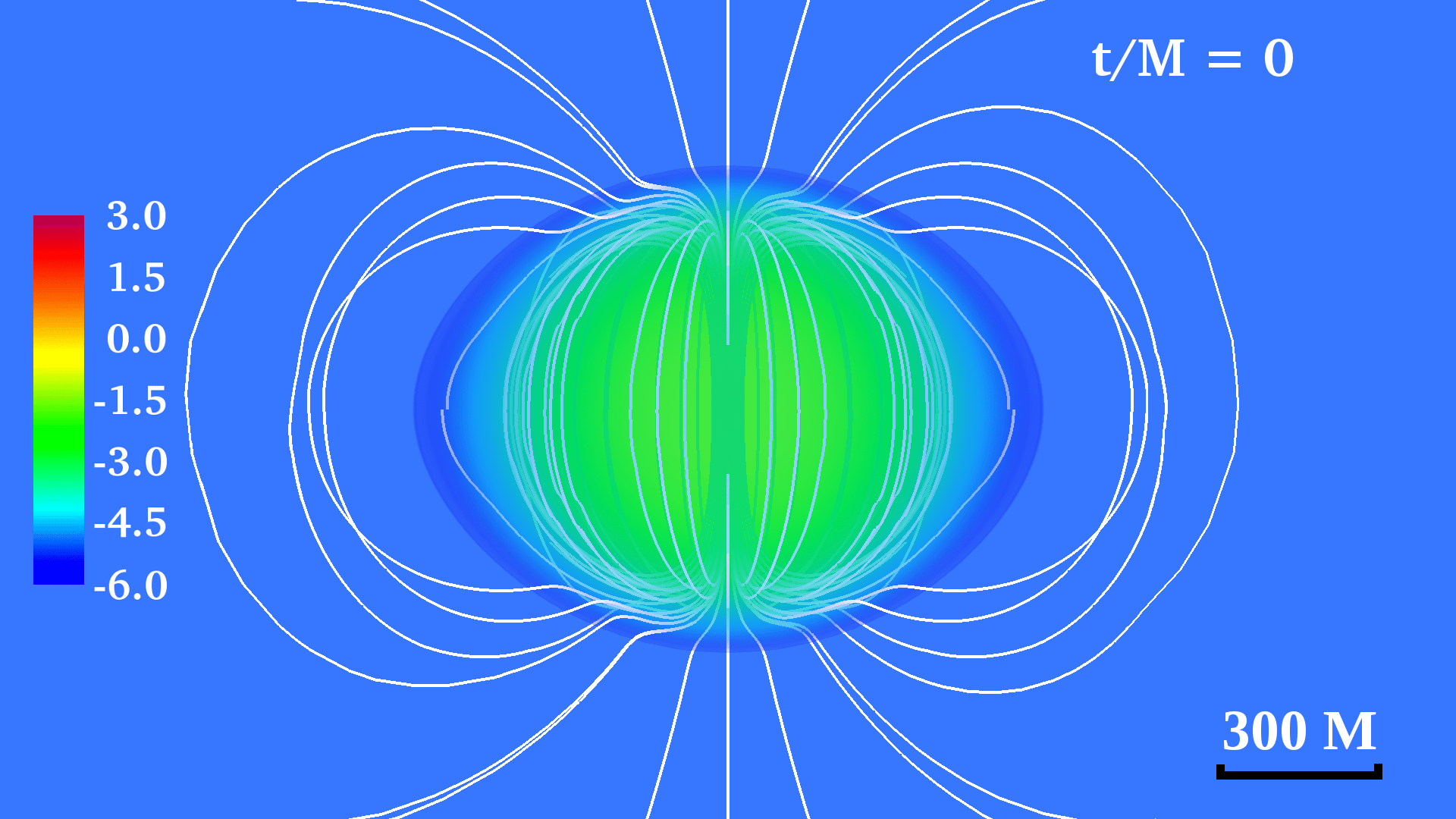
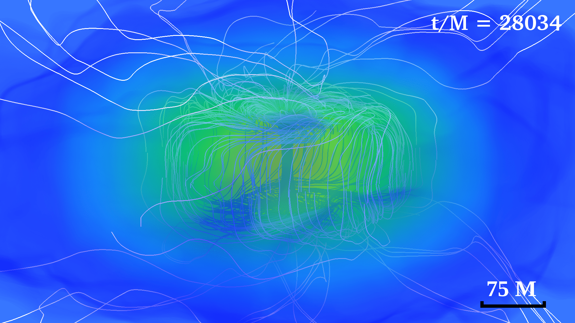
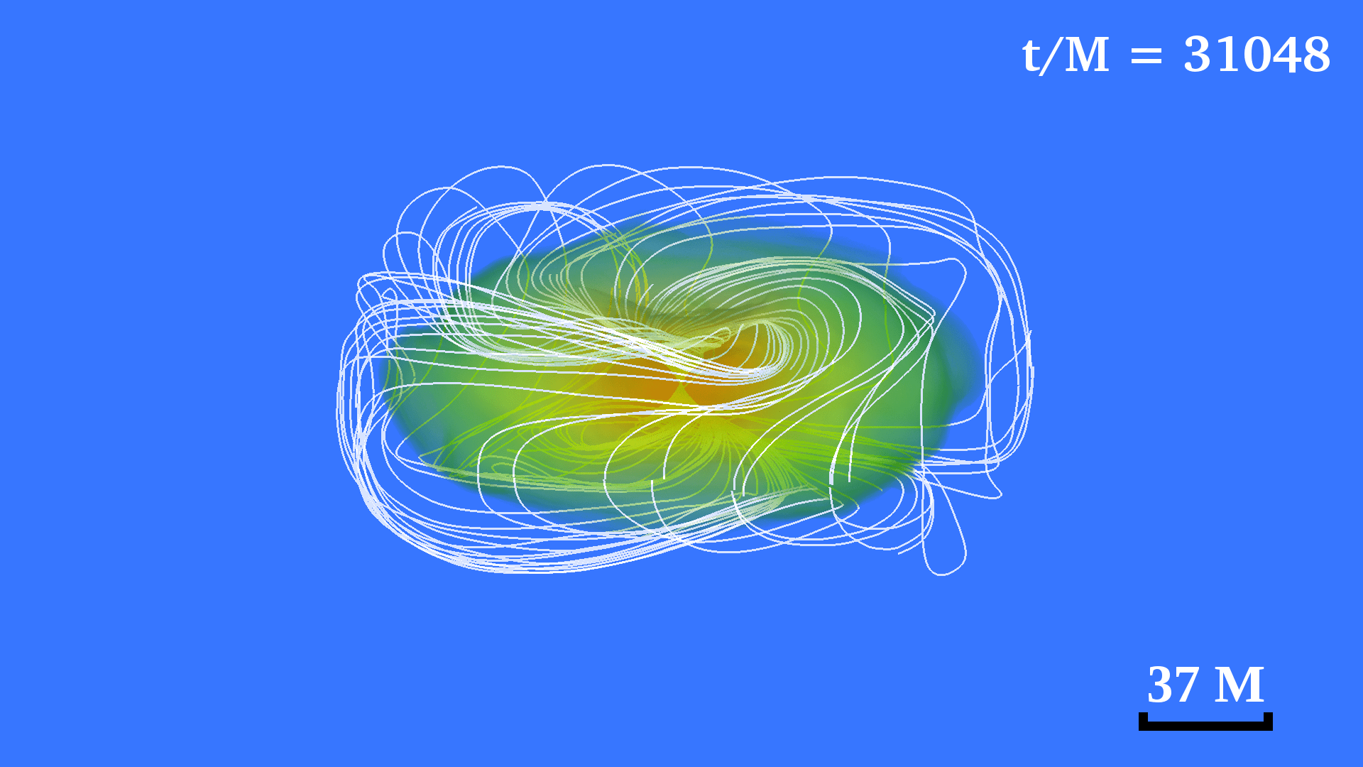
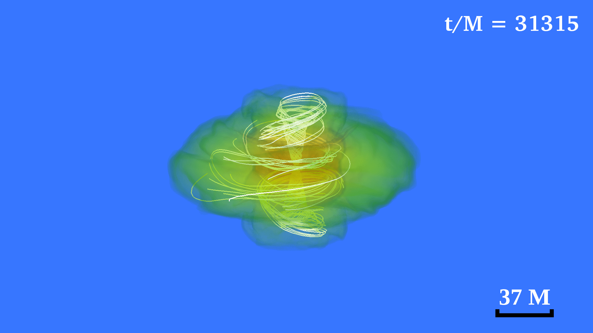
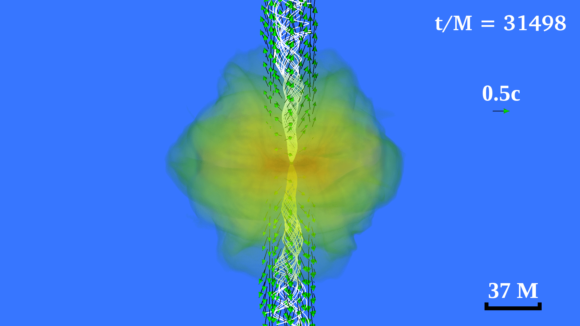
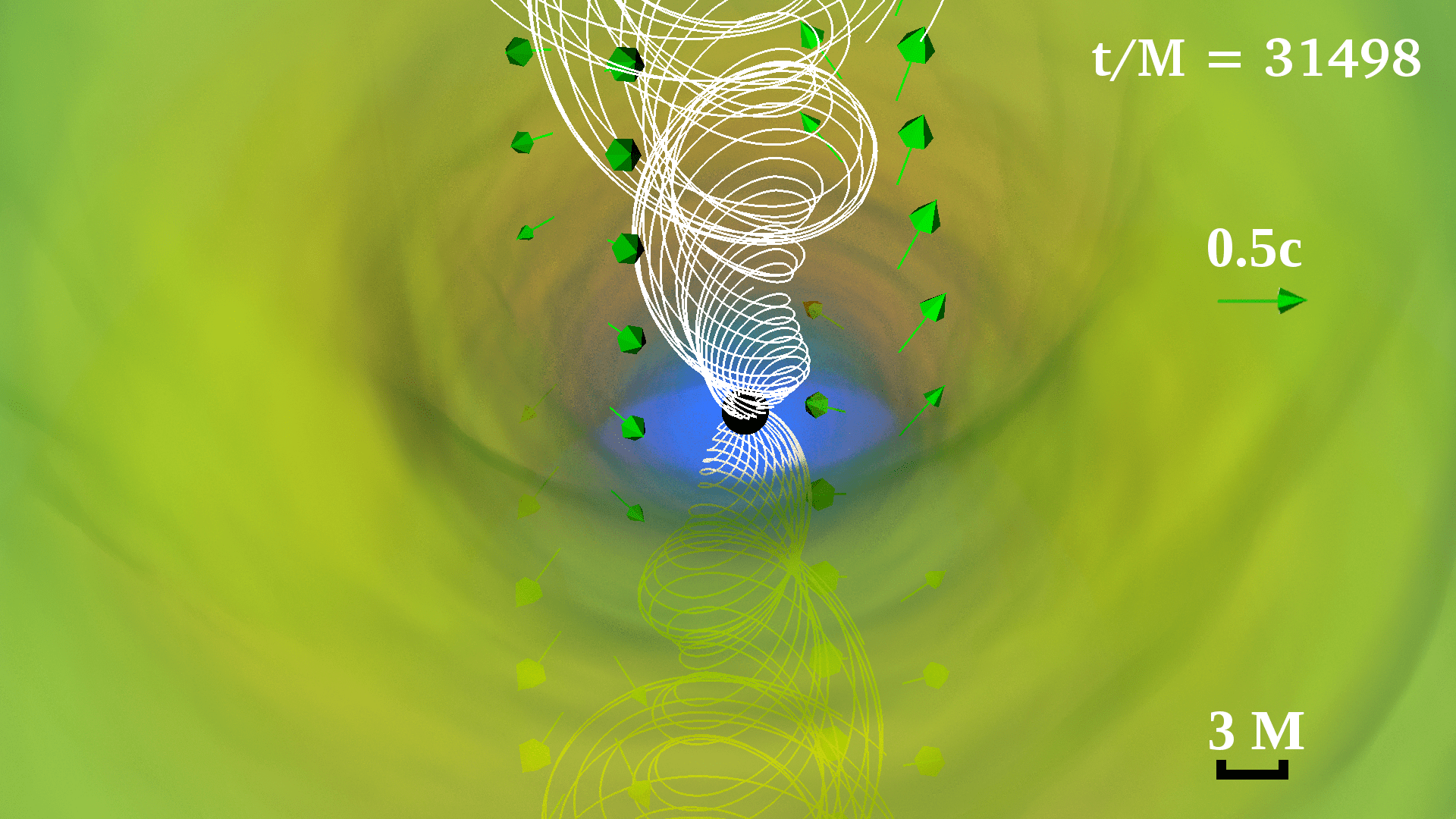
Figure 1: Volume rendering of the rest-mass density normalized to its initial maximum value $\rho_{0,\text{max}}=9.9\times 10^{-2}(M/10^{6}M_{\odot})^{-2}\,{\rm g}\,{\rm cm}^{-3}$ (log scale) at select times for the $\rm S_{\rm{\tiny{Int+Ext}}}$ case. Solid lines indicate the magnetic-field lines, and arrows show plasma velocities with length proportional to their magnitude. The bottom left panel displays the collimated, helical magnetic field and outgoing plasma, whose zoomed-in view near the horizon is shown in the bottom right panel. Here $M=4.9(M/10^{6}M_{\odot}){\rm s}=1.47\times 10^{6}(M/10^{6}M_{\odot})\rm km$.

II Methods

In this section we describe in detail our initial data, the numerical method and the grid structure we employ for solving the Einstein equations coupled to the equations of ideal magnetohydrodynamics in a dynamical, curved spacetime. We also summarize the diagnostics we adopt to monitor the simulations.

II.1 Initial data

To model a collapsing SMS, and also to crudely model the collapse of a Pop III star, we start with a marginally unstable $\Gamma=4/3$ polytrope that is uniformly rotating at the mass-shedding limit. The rotating polytropic star is built with the code of Cook et al. (1992, 1994). We employ dimensionless (barred) variables in which, for instance, the radius $R$, mass $M$ and density $\rho$ are scaled as follows Baumgarte and Shapiro (2010)

$$\bar{R}= \kappa^{-n/2}\,R,\qquad\bar{M}= \kappa^{-n/2}\,M,\qquad\bar{\rho}=\kappa^{n}\,\rho\,,$$ (1)

where $n=1/(\Gamma-1)$ is the polytropic index. Our calculations scale with the polytropic constant $\kappa$. The polytropic model we adopt has the same initial properties as the one in Liu et al. (2007), and it is characterized by the following parameters: ADM mass $\bar{M}_{\rm ADM}=4.572$, central rest-mass density $\bar{\rho}_{0,c}=7.7\times 10^{-9}$, dimensionless angular momentum $J/M^{2}=0.96$, and ratio of kinetic to gravitational-binding energy $T/|W|=0.009$. The equatorial radius of the star is $R_{\rm eq}=626M_{\rm ADM}\approx 9.25\times 10^{6}\,({M_{\rm ADM}}/{10^{6}M_{\odot}})$km. This model is marginally unstable to collapse.

We consider three different initial scenarios as follows:

• Case $\rm S_{\rm{\tiny{Int+Ext}}}$: Magnetized configuration in which the initial equilibrium star is seeded with a dipole-like magnetic field which extends from the stellar interior into the exterior (see top left panel in Fig. 1),

• Case $\rm S_{\rm{\tiny{Int}}}$: Magnetized configuration in which the initial equilibrium star is seeded with a poloidal magnetic field confined to the stellar interior (see top left panel in Fig. 2),

• Case $\rm S_{\rm{\tiny{Hydro}}}$: Purely hydrodynamic configuration (see bottom left panel in Fig. 2).

Table 1: Summary of the initial model parameters. Here ${\mathcal{M}}/{T}$ is the ratio of the magnetic to the rotational kinetic energy, $\bar{B}$ is the magnetic-field strength computed via Eq. (5) and $\beta^{-1}_{\rm ext}$ is the magnetic to gas pressure ratio in the stellar exterior.

Case	${\mathcal{M}}/{T}$	$\bar{B}\times({M}/{10^{6}\,M_{\odot}})$G	$\beta^{-1}_{\rm ext}$
$\rm S_{\rm{\tiny{Int+Ext}}}$	0.1	$6.5\times 10^{6}$	100
$\rm S_{\rm{\tiny{Int}}}$	0.1	$6.5\times 10^{6}$	0
$\rm S_{\rm{\tiny{Hydro}}}$	0	0	0

The magnetic field in the magnetized configurations we consider is generated by the two-component vector potential

$$A_{\phi}=e^{-(r/r_{1})^{2p}}A^{(1)}_{\phi}+\left(1-e^{-(r/r_{1})^{2p}}\right)\,A^{(2)}_{\phi}\,,$$ (2)

where $r^{2}=(x-x_{\text{\tiny{SMS}}})^{2}+(y-y_{\text{\tiny SMS}})^{2}+z^{2}$ with ($x_{\text{\tiny SMS}}$, $y_{\text{\tiny SMS}})$ the coordinates of the center of mass of the star. The constants $r_{1}$ and $p$ are free parameters that control the radial position and the width of the transition region between the two vector potentials $A^{(1)}_{\phi}$ and $A^{(2)}_{\phi}$. The vector potential $A^{(1)}_{\phi}$ is given by

$$A^{(1)}_{\phi}=A_{b}\,\varpi^{2}\,\text{max}(P-P_{\text{cut}},0)^{n_{b}}\,,$$ (3)

with $\varpi^{2}=(x-x_{\text{\tiny SMS}})^{2}+(y-y_{\text{\tiny SMS}})^{2}$, $P_{\rm cut}$ the cutoff pressure that confines the magnetic field to a region where $P>P_{\rm cut}$, and $A_{b}$ the constant that adjusts the initial magnetic-field strength. Here $A^{1}_{\phi}$ is used for seeding a poloidal magnetic field for the $S_{\rm Int}$ case; i.e., effectively we set $r_{1}=\infty$ in Eq. (2). Vector potentials of this type with $n_{b}=1$ have been used for studying magnetized accretion disks around stationary black holes McKinney and Gammie (2004); Villiers et al. (2003) and in compact binary mergers involving neutron stars (see, e.g. Ref.  Etienne et al. (2012a) and references therein), but here we set $n_{b}=1/8$ to approximate the interior magnetic-field configuration that was adopted in Liu et al. (2007). For the case $\rm S_{\rm{\tiny{Int}}}$ we set $P_{\rm cut}=10^{-4}P_{\rm max}$, with $P_{\rm max}$ being the maximum value of the pressure at $t=0$. For the case $\rm S_{\rm{\tiny{Int}}}$ we use a standard constant-density atmosphere with rest-mass density $\rho_{0,\,{\rm atm}}=10^{-10}\,\rho_{0,\,\rm max}$, where $\rho_{0,\,\rm max}$ is the maximum value of the rest-mass density at $t=0$.

The vector potential $A^{(2)}_{\phi}$ is given by Paschalidis et al. (2013)

$$A^{(2)}_{\phi}=\frac{\pi\,r_{0}^{2}\,I_{0}\,\varpi^{2}}{(r^{2}_{0}+r^{2})^{3/2}}\,\left(1+\frac{15\,r_{0}^{2}\,(r^{2}_{0}+\varpi^{2})}{8(r^{2}_{0}+r^{2})^{2}}\right)\,,$$ (4)

and approximates the magnetic field generated by a current loop, which becomes a dipole at large distances. Here $r_{0}$ and $I_{0}$ are the loop radius and current, and they determine the geometry and strength of the magnetic field.

For the $\rm S_{Int+Ext}$ case we use the superposition of the two vector potentials because $A^{(2)}_{\phi}$ alone does not appear to have enough degrees of freedom to allow us to specify both the total magnetic energy and the value of the plasma parameter $\beta$ in the stellar exterior as we discuss below. The form (2) guarantees a rapid and smooth transition of the magnetic field from $A^{(1)}_{\phi}$ in the stellar interior to $A^{(2)}_{\phi}$ in the exterior (see top left panel in Fig. 1). We adopt $P_{\rm cut}=10^{-4}P_{\rm max}$, $r_{0}\approx 2.2M$, $r_{1}\approx 240M$, and $p=2$. Although this choice of superposed vector potentials does not necessarily correspond to a realistic distribution of currents, it allows a fairer comparison with the interior-only case because the bulk of the interior magnetic field in the $S_{\rm Int+Ext}$ case is practically the same as in the $S_{\rm Int}$ case, and any differences arise because of the exterior component. Following Paschalidis et al. (2015), to mimic a force-free magnetosphere in the stellar exterior and to reliably evolve the magnetic field outside the star in the $S_{\text{Int+Ext}}$ case, at $t=0$ we set a low and variable density atmosphere in the exterior such that the magnetic to gas pressure ratio is $\beta^{-1}_{\rm ext}=100$.

We set $A_{b}=2.91\times 10^{-7}$, $I_{0}=7.35\times 10^{-3}$ for the $\rm S_{Int+Ext}$ case, and $A_{b}=1.26\times 10^{-6}$, $I_{0}=2.25\times 10^{-3}$ for the $\rm S_{Int}$ case. These values fix the ratio of magnetic to rotational kinetic energy $\mathcal{M}/T$ to be 0.1 (corresponding to $\mathcal{M}/|W|=9\times 10^{-4}$). Hence, the magnetic field is dynamically unimportant initially. We compute the magnetic energy as measured by a normal observer $\mathcal{M}$ through Eq. (30) of Liu et al. (2007). Table 1 summarizes the initial parameters of our models.

The resulting averaged magnetic-field strength $\bar{B}$ is

$$\bar{B}\equiv\sqrt{8\,\pi\,\mathcal{M}/V_{s}}=6.5\times 10^{6}\,\left(\frac{M}{10^{6}\,M_{\odot}}\right)\rm G\,,$$ (5)

which matches the initial averaged magnetic-field strength used in Liu et al. (2007). Here $V_{s}=\int\sqrt{\gamma}\,d^{3}x$ is the proper volume of the star at $t=0$, and $\gamma$ is the determinant of the three-metric $\gamma_{ij}$.

To accelerate the collapse, at $t=0$ the pressure is depleted by $1\%$ for all three cases.

II.2 Evolution

We use the Illinois GRMHD adaptive mesh refinement (AMR) code embedded in the Cactus/Carpet infrastructure Cactus Website ; Carpet Website . Note that this code is different than its publicly available counterpart embedded in the Einstein Toolkit Etienne et al. (2015). This code has been widely tested and used in different scenarios involving compact objects and/or magnetic fields (see, e.g. Refs.  Etienne et al. (2008); Liu et al. (2008); Paschalidis et al. (2011a, b); Etienne et al. (2012a); Gold et al. (2014, 2014)). For implementation details see Etienne et al. (2010); Etienne et al. (2012b); Etienne et al. (2012).

The Illinois code solves the equations of ideal GRMHD in a flux conservative formulation [see Eqs. (27)–(29) in Etienne et al. (2010)] via high-resolution shock capturing methods Duez et al. (2005). To guarantee that the magnetic field remains divergenceless, the code solves the magnetic induction equation via a vector potential formulation [see Eqs. (8) and (9) in Etienne et al. (2012)]. We adopt the generalized Lorenz gauge Etienne et al. (2012); Farris et al. (2012) to close Maxwell’s equations, and employ a damping parameter $\xi=4.6/M$, where $M$ the ADM mass of the system. This EM gauge choice avoids the development of spurious magnetic fields that arise due to interpolations across AMR levels (see Etienne et al. (2012) for more details).

The GRMHD evolution equations are closed by employing a $\Gamma$-law EOS, $P=(\Gamma-1)\,\epsilon\,\rho_{0}$, which allows for shock heating. Here $\epsilon$ is the specific internal energy and $\rho_{0}$ the rest-mass density. In all our models we set $\Gamma=4/3$, which is appropriate when thermal radiation pressure dominates Baumgarte and Shapiro (1999).

To evolve the spacetime metric, we use the Baumgarte-Shapiro-Shibata-Nakamura formulation of Einstein’s equations Shibata and Nakamura (1995); Baumgarte and Shapiro (1998) coupled to the moving puncture gauge conditions Baker et al. (2006); Campanelli et al. (2006) with the equation for the shift vector cast in first-order form (see, e.g. Refs.  Hinder et al. (2014); Ruiz et al. (2011)). The shift vector parameter $\eta$ is set to $\eta=4.6/M$.

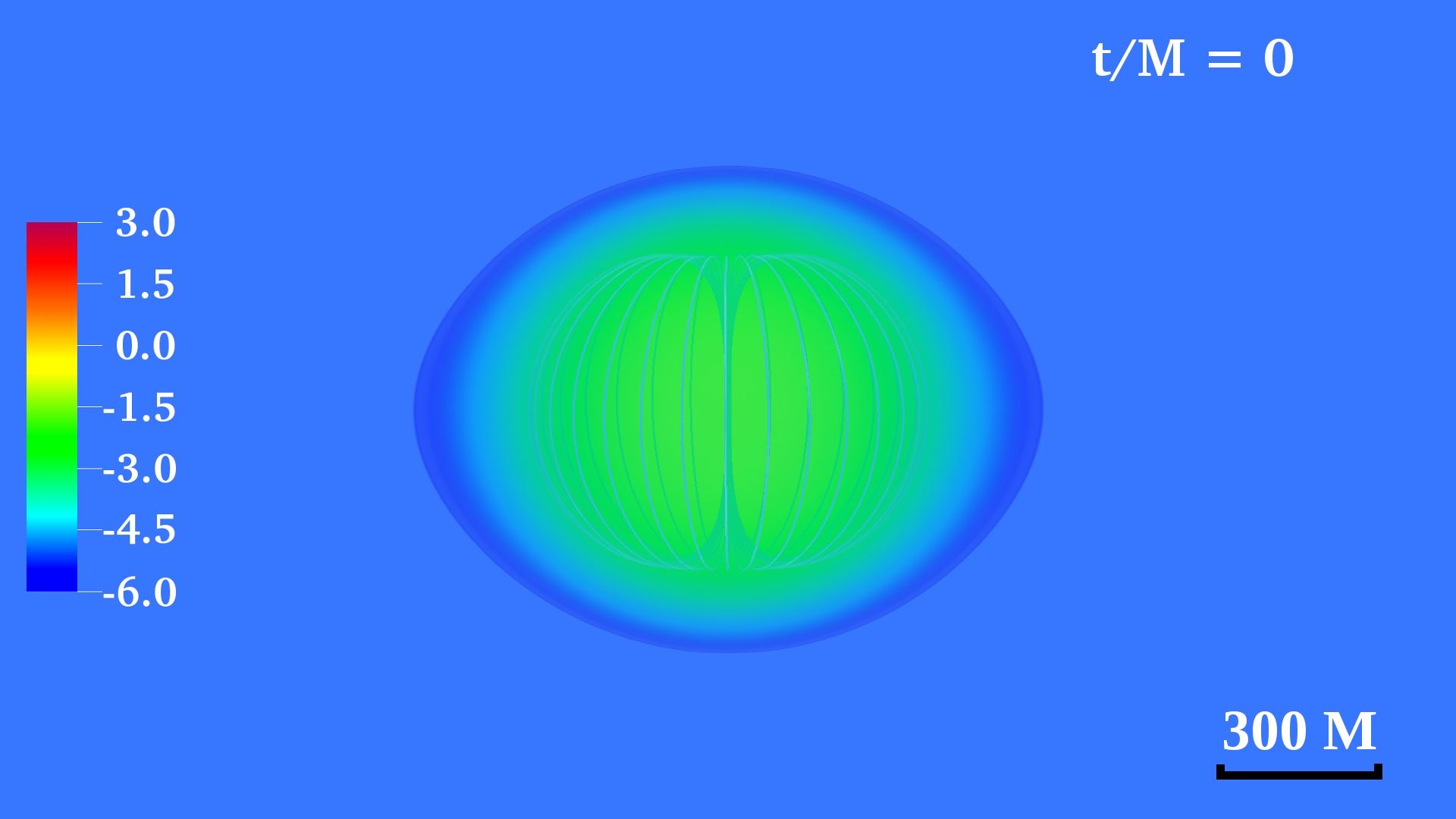
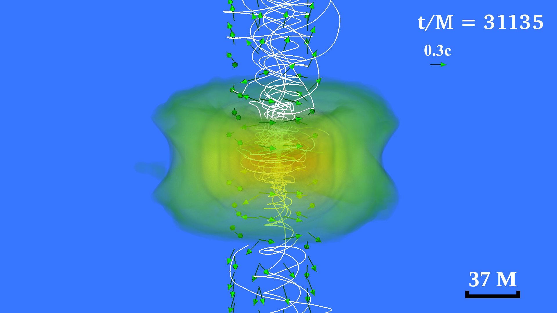
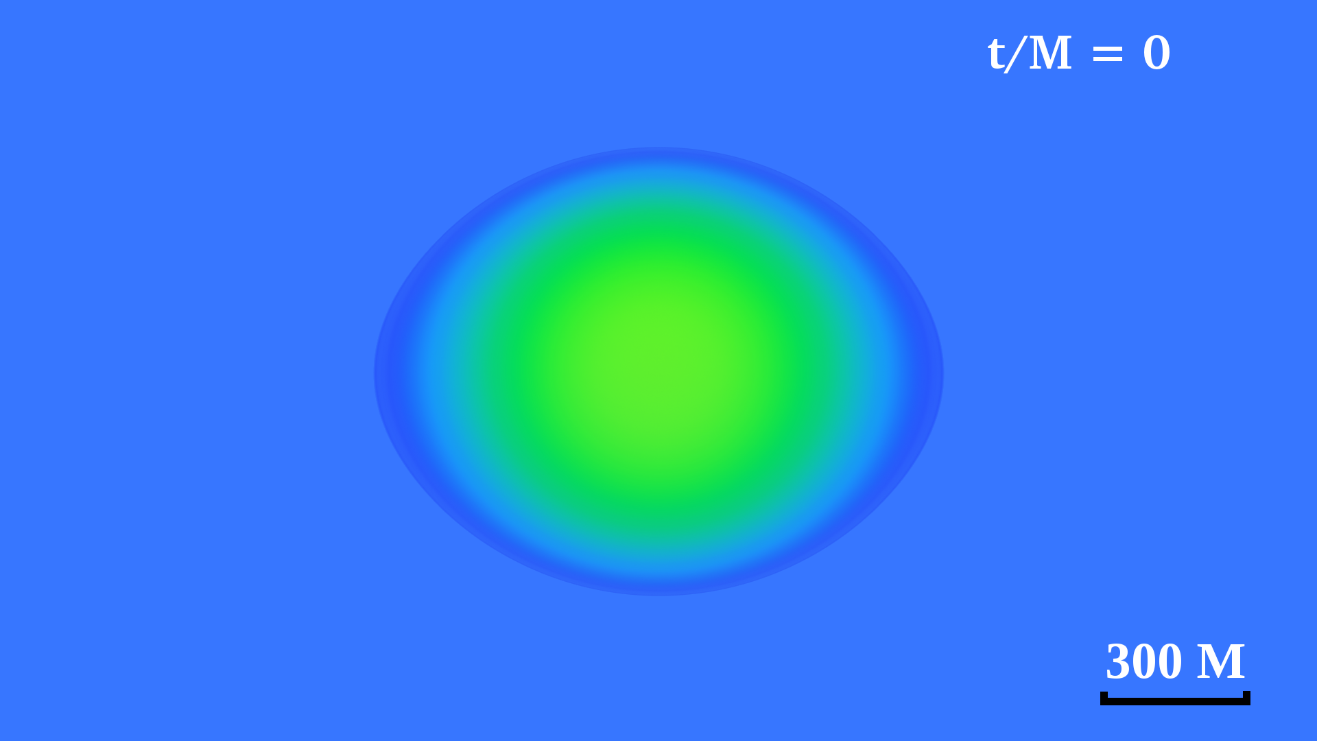
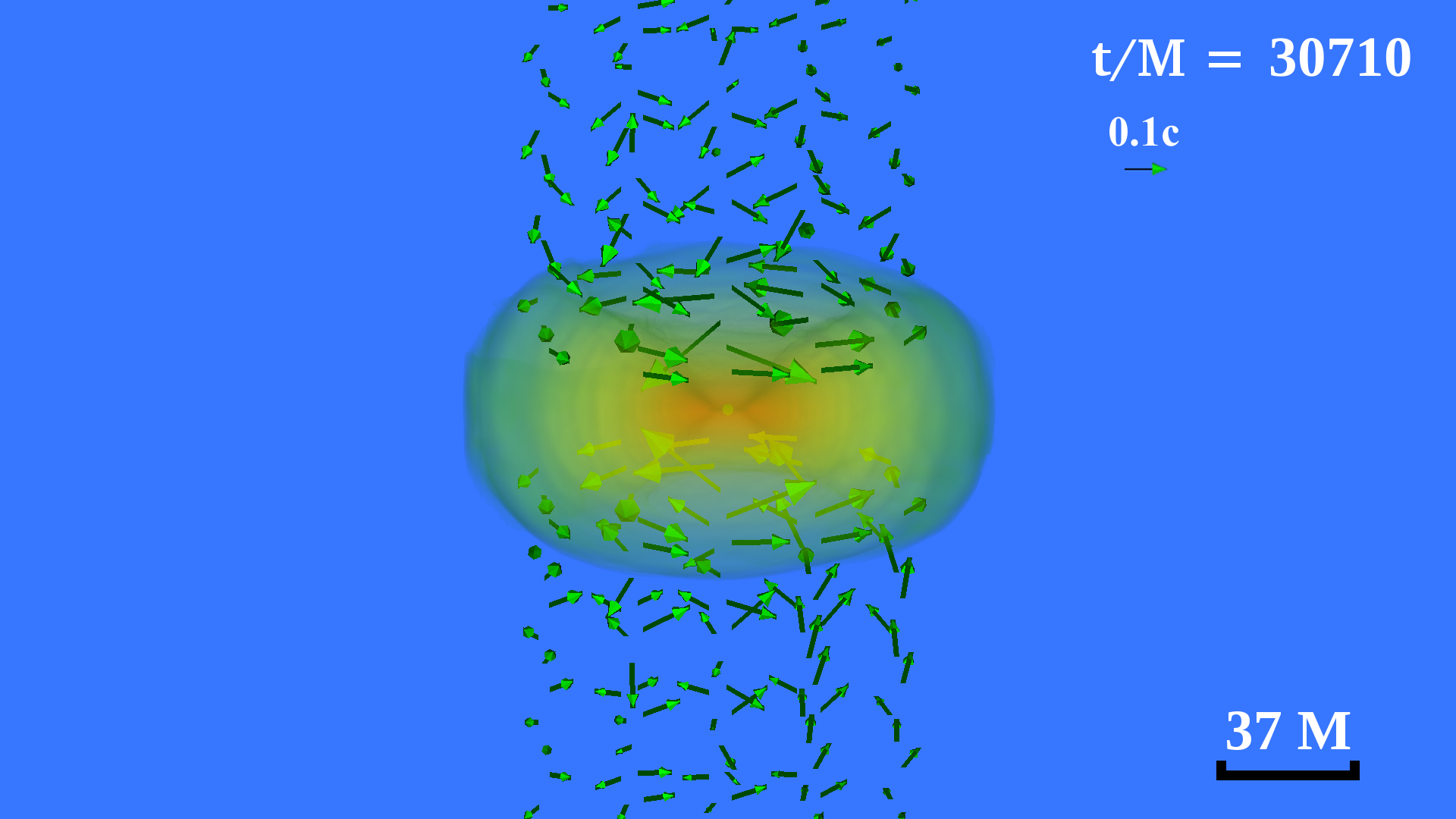
Figure 2: Volume rendering of the rest-mass density normalized to its initial maximum value (log scale) for the case $\rm S_{\rm{\tiny{Int}}}$ (top row) and the case $\rm S_{\rm{\tiny{Hydro}}}$ (bottom row). Initial and final configurations for these two cases are shown in the left and right panels, respectively. Solid lines indicate the magnetic-field lines, and arrows show plasma velocities with length proportional to their magnitude. Here $M=4.9(M/10^{6}M_{\odot}){\rm s}=1.47\times 10^{6}(M/10^{6}M_{\odot})\rm km$.

II.3 Grid structure

During collapse, the equatorial radius of the star shrinks from $\sim 630M$ to a few $M$. To follow the evolution efficiently we add high-resolution refinement levels as the collapse proceeds. This same approach was also adopted in Shibata and Shapiro (2002); Liu et al. (2007). In all the cases listed in Table 1, we begin the numerical integrations by using a set of five nested refinement levels differing in size and resolution by factors of 2. The base level has a half-side length of $1312M\approx 2.1\,R_{\rm eq}\approx 1.9\times 10^{9}(M/{10^{6}M_{\odot}})$km, which sets the location of the outer boundary. The grid spacing on the base level is $21.8M=3.22\times 10^{7}(M/{10^{6}M_{\odot}})$km. To save computational resources, reflection symmetry across the equatorial plane is imposed. The resulting number of grid points per level is $N=120^{2}\times 60$. To maintain high resolution throughout the collapse, we add a new refinement level with the same number of grid points $N$, and half the grid spacing of the previous highest-resolution level every time the density increases by a factor of 3. Such a procedure is repeated 5 times for the $\rm S_{\rm{\tiny{Hydro}}}$ case and 6 times for the $\rm S_{\rm{\tiny{Int}}}$ and $\rm S_{\rm{\tiny{Int+Ext}}}$ cases.

Thus, in the last stages of the collapse the grid structure consists of a total of eleven (ten) nested refinement levels in the MHD (hydrodynamic) evolutions, in which the finest level has grid spacing of $\sim 0.021M=3.1\times 10^{4}(M/{10^{6}M_{\odot}})$km [$\sim 0.042M=6.2\times 10^{4}(M/{10^{6}M_{\odot}})$km]. The highest resolution on our grids is similar to that used in the axisymmetric simulations of Liu et al. (2007), but now our simulations are in 3+1 dimensions. The main purpose of applying higher resolution in the magnetized cases is to more accurately evolve the low-density, near force-free environments that emerge above the black hole poles.

II.4 Diagnostics

As a check on the validity of the numerical integration we monitor the Hamiltonian and momentum constraints computed in Eqs.(40) and (41) in Etienne et al. (2008). In all our cases, the normalized constraint violations remain below $1\%$ over the entire evolution. We also check the conservation of the rest mass $M_{0}$, and monitor the ADM mass $M$ and the ADM angular momentum $J$. These quantities are computed by performing the ADM mass and angular momentum integrals via Eqs. (21) and (22) in Etienne et al. (2012b) over the surface of coordinate spheres. A fraction of the system’s mass and angular momentum are radiated away through gravitational and EM radiation as well as by escaping matter. The dominant loss through our outermost extraction sphere is via escaping matter (see Table  2), but that corresponds to only $1\%$ of the ADM mass by the end of our simulations. Therefore, we are reassured to find that the ADM mass is conserved to $\sim 1\%$, and that the ADM angular momentum is conserved to $\sim 2\%$ in all of our cases.

We use our modified version of the Psikadelia thorn to extract GWs through the Weyl scalar $\Psi_{4}$, which is decomposed into $s=-2$ spin-weighted spherical harmonics (see, e.g. Refs.  Ruiz et al. (2008)). We estimate the thermal energy generated by shocks through the entropy parameter $K\equiv P/P_{0}$, where $P_{0}=\kappa\,\rho_{0}^{\Gamma}$ is the pressure associated with the unshocked EOS. The specific internal energy has a “cold” $\epsilon_{0}$ and a “thermal” component $\epsilon_{\rm th}$, i.e., $\epsilon=\epsilon_{0}+\epsilon_{\rm th}$ with Etienne et al. (2009)

$$\epsilon_{0} =-\int P_{0}\,d(1/\rho_{0})=\frac{\kappa}{\Gamma-1}\,\rho_{0}^{\Gamma-1}\,.$$ (6)

Using the $\Gamma$-law EOS, it is straightforward to show that $\epsilon_{\rm th}=(K-1)\,\epsilon_{0}$. Thus, for shock-heated gas ($\epsilon_{\rm th}>0$) the entropy parameter always satisfies $K>1$ Etienne et al. (2009).

We adopt the AHFinderDirect thorn Thornburg (2004) to locate the apparent horizon (AH) following BH formation, and we use the isolated horizon formalism to estimate the dimensionless spin parameter $a_{\rm BH}/M_{\rm BH}$ and mass $M_{\rm BH}$ of the BH Dreyer et al. (2003).

Finally, following BH formation the outgoing EM luminosity is computed as in Paschalidis et al. (2013); Ruiz et al. (2012) through the following surface integral:

$$L_{\rm EM}=\lim_{r\rightarrow\infty}\int r^{2}\,S^{\hat{r}}\,d\Omega\,.$$ (7)

The surfaces of integration are spheres of constant coordinate radii at large distances from the BH. Here $S^{\hat{r}}$ is the Poynting vector $\mathbf{S}=(\mathbf{E}\times\mathbf{B})/4\pi$ projected onto the outgoing unit vector $\hat{r}$.

Table 2: Summary of key results. Here $t_{\rm BH}$ is the coordinate time at which the apparent horizon appears, $M_{\rm BH}$ and $a_{\rm BH}/M_{\rm BH}$ are the mass and dimensionless spin parameter of the BH after they settle down (at $t-t_{\rm BH}\sim 150M$), $M_{\rm esc}$ is the rest mass of unbound matter, $M_{\rm disk}$ is the rest mass outside the horizon minus the unbound mass, and $\dot{M}$ is the rest-mass accretion rate. The last two quantities have been computed after the accretion rate has settled, and $\tau_{\rm disk}=M_{\rm disk}/\dot{M}$ is the disk lifetime. The quantities $t_{\rm BH}$ and $\tau_{\rm disk}$ are normalized by $(M/10^{6}M_{\odot})$, and $\Gamma_{L}$ is an average Lorenz factor within the funnel. For the $\rm S_{\rm{\tiny{Int+Ext}}}$ case $\Gamma_{L}$ is quoted at the time when the ratio $b^{2}/(8\pi\,\rho_{0})\sim 200$ above the BH poles, where $b$ is the magnetic-field strength measured by an observer comoving with the plasma. For the $\rm S_{\rm{\tiny{Int}}}$ case $\Gamma_{L}$ is quoted near the end of the simulation, $L_{\rm EM}$ is the time-averaged Poynting luminosity over the last $300M$ before we terminate our simulations, and $L_{\rm GW}$ is the time-averaged GW luminosity over the duration of the GW burst $\Delta t_{\rm GW}\simeq 80M$. In the magnetized cases, the anticipated total energy removed by EM processes, $E_{\rm EM}\sim L_{\rm EM}\times\tau_{\rm disk}\sim 10^{-5}-10^{-3}M$, exceeds the total energy lost in GWs $E_{\rm GW}\simeq 10^{-6}M$.

Model	$t_{\rm BH}$	$M_{\rm BH}/M$	$a/M_{\rm BH}$	$M_{\rm esc}/M$	$M_{\rm disk}/M$	$\dot{M}(M_{\odot}/s)$	$\tau_{\rm disk}$	$\Gamma_{L}$	$L_{\rm EM}$ erg/s	$L_{\rm GW}$ erg/s
$\rm S_{\rm{\tiny{Int+Ext}}}$	$1.5\times 10^{5}$s	0.91	0.71	$1.1\%$	$7.0\%$	1.11	$7.2\times 10^{4}$s	1.20	$10^{52.5}$	$4.7\times 10^{51}$
$\rm S_{\rm{\tiny{Int}}}$	$1.5\times 10^{5}$s	0.92	0.75	$0.9\%$	$6.0\%$	1.20	$5.0\times 10^{4}$s	1.20	$10^{50.6}$	$4.7\times 10^{51}$
$\rm S_{\rm{\tiny{Hydro}}}$	$1.4\times 10^{5}$s	0.92	0.75	$0.2\%$	$9.0\%$	1.0	$9.0\times 10^{4}$s	-	-	$4.7\times 10^{51}$

III Results

The early stages of the evolution are similar for all three cases we consider. Thus, we focus the discussion on the $\rm S_{\rm{\tiny{Int+Ext}}}$ case, unless otherwise specified. Key results from all cases are summarized in Table 2.

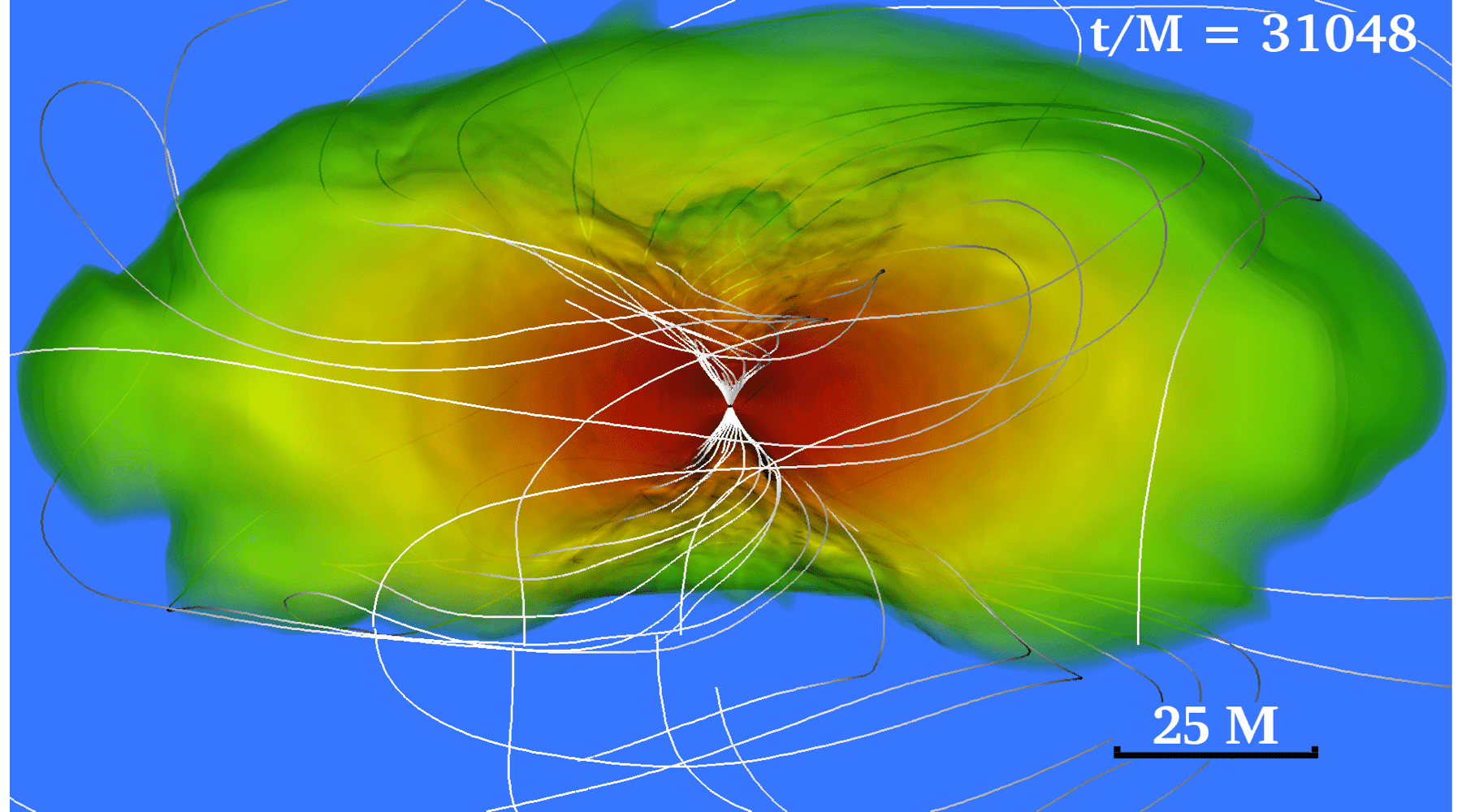
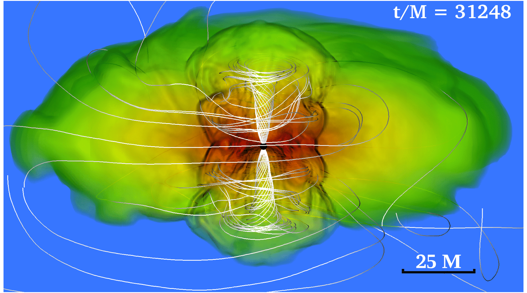
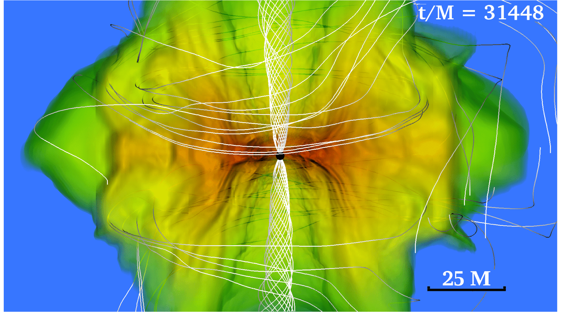
Figure 3: Meridional cut of 3D density profile for the $\rm S_{\rm{\tiny{Int+Ext}}}$ case at $t-t_{\rm{BH}}=\text{ 0, 200}M\text{, and 400}M$, with magnetic-field lines in white. The top panel corresponds to the time near BH formation. The middle panel shows the shock front propagating outward along which the entropy parameter $K$ becomes $>1$. The shock drives an outflow which eventually becomes a magnetically supported and confined incipient jet (bottom panel).

Following the initial pressure depletion the star undergoes collapse (top right panel in Fig. 1). As the gas falls inward, the density in the stellar interior increases. By about $t\sim 1.3\times 10^{4}M\simeq 6.4\times 10^{4}(M/10^{6}M_{\odot}){\rm s}$ we observe the formation of an inner core that undergoes rapid collapse. Similar behavior was found in the Newtonian simulations of a $\Gamma=4/3$ polytrope in Goldreich and Weber (1980). In addition to the increasing matter density, we observe that during the last stages of the collapse the frozen-in magnetic-field lines are compressed and become wound (middle, left panel in Fig. 1), and the magnetic energy builds up rapidly and is amplified by a factor of $\sim 100$ until a BH forms. During this period, we resolve the wavelength of the fastest-growing magnetorotational-instability (MRI) mode by $\gtrsim 10$ points—the rule-of-thumb for capturing MRI Shibata et al. (2006). MRI acts as an effective viscosity driving turbulence and thus helps maintain the accretion of gas onto the BH once the system reaches quasistationary equilibrium. In the early stages immediately following collapse, however, hydrodynamical forces drive the accretion, and the rate for the pure hydrodynamical and magnetic-field cases are comparable. MRI also contributes to the amplification of the poloidal magnetic field, while magnetic winding amplifies the toroidal component. This amplification occurs both in the disk and above the BH poles.

The AH appears approximately at the same time $t_{\rm BH}$ in all cases, which is expected because the seed magnetic field is dynamically unimportant initially. Right after the AH appearance, the mass and spin of the remnant BH evolve rapidly as the surrounding gas is accreted. Following this high-accretion episode, the rapid growth of the BH settles at about $t-t_{\rm BH}\sim 150M\approx 740(M/10^{6}M_{\odot})$s. At this time the values of the BH mass and dimensionless spin are $M_{\rm BH}\approx 0.91M$ and $a_{\rm BH}/M_{\rm BH}\approx 0.71$ for the $\rm S_{\rm{\tiny{Int+Ext}}}$ case, and $M_{\rm BH}\approx 0.92M$ and $a_{\rm BH}/M_{\rm BH}\approx 0.75$ for the other two cases (see Table 2). These values are consistent with those of the previous axisymmetric calculations of Shibata and Shapiro (2002); Liu et al. (2007).

Following BH formation, high-angular-momentum gas originating in the outer layers of the star begins to settle in an accretion torus around the BH (see middle left panel in Fig 1). During this phase, a substantial amount of gas descends towards the BH, which increases the density in the torus. The rapidly swirling, dense gas soon forms a centrifugal barrier onto which additional infalling matter collides, and ultimately a reverse shock is launched at $t-t_{BH}\sim 170M=830(M/10^{6}M_{\odot})$s (see Fig. 3). The shock increases the entropy of the gas and pushes the fluid outward. This initial outflow ultimately turns into a wind which is almost isotropic. The entropy parameter $K$ exceeds 1 in all three cases.

In the hydrodynamic case the shock-driven, isotropic outflow disappears after $t\sim 1100M$ (see bottom right panel in Fig. 2). By contrast, in the magnetized cases the initial outflow develops into one with two components: an isotropic, pressure-dominated wind component, and a collimated, mildly relativistic, Poynting-dominated component—an incipient jet. In particular, the magnetic-field lines anchored into the initial shock-driven outflow are stretched, forming a poloidal component, and they become more tightly wound (see middle right panel in Fig 1). Magnetic winding converts poloidal to toroidal flux and builds up magnetic pressure above the BH poles in a similar fashion as discussed in Paschalidis et al. (2015) for black hole–neutron star mergers. Eventually, the growing magnetic pressure gradients become so strong that an outflow is launched and sustained by the helical magnetic fields. During this period, the magnetic field above the BH pole reaches a value of $\sim 4.0\times 10^{10}({10^{6}M_{\odot}/M})$G and remains roughly constant.

As the magnetic pressure above the BH poles increases for $t>t_{\rm BH}$, magnetically dominated regions where $b^{2}/(8\pi\rho_{0})>1$ (where $b$ is the magnetic-field strength measured by an observer comoving with the plasma) expand outwards above the BH poles, forming an incipient jet (see collimated, helical magnetic field in the bottom left panel in Fig 1 and top right panel in Fig. 2). Based on the distribution of the outgoing flux on the surface of the distant sphere we estimate that the half-opening angle of the jet is $\sim 25^{\circ}$. We define the jet half-opening angle, as the polar angle $\theta_{0}$ at which the Poynting flux drops to $50\%$ of the maximum. In contrast to the hydrodynamic case, in the magnetized cases the outflow persists until we terminate our simulations because it is driven by the magnetic field.

The characteristic value of the Lorentz factor measured by a normal observer at large distances ($\Gamma_{L}=\alpha\,u^{0}$, with $\alpha$ being the lapse function) in the funnel is $\Gamma_{L}\approx 1.2$. The outflow is therefore mildly relativistic. However, the value of the magnetization in the funnel becomes $b^{2}/(8\pi\rho_{0})\gtrsim 100$. This is shown in Fig. 4 which displays a volume rendering of the magnetization at $t-t_{\rm BH}\approx 450M\approx 2200(M/10^{6}M_{\odot})$s. Highly magnetized regions extend to $\gtrsim 50M\approx 50r_{\rm BH}$ above the BH poles (here $r_{\rm BH}$ is the apparent horizon radius). The ratio $b^{2}/(8\pi\rho_{0})$ equals the terminal Lorentz factor in axisymmetric, steady-state, magnetically dominated jets Vlahakis and Königl (2003). Thus, the incipient jets found here, in principle, can be accelerated to typical Lorentz factors required by GRB observations Gehrels and Razzaque (2013). However, the terminal Lorentz factor is anticipated to be reached at hundreds of thousands to millions of $M$ away from the engine Tchekhovskoy et al. (2007); Paschalidis (2017) outside of our computational domain. We note that although our code may not be reliable at values of $b^{2}/(8\pi\rho_{0})\gtrsim 200$, the increase in the magnetization in the funnel is robust (see discussions in Paschalidis et al. (2015); Ruiz et al. (2016)). As in Paschalidis et al. (2015); Ruiz et al. (2016), to ensure the physical nature of the jet, we track Lagrangian particle tracers and ensure that the matter in the jet is being replenished by plasma originating in the torus and not in the artificial atmosphere.

In all three cases outgoing matter ($v^{r}=u^{r}/u^{0}>0$) in the jet funnel and wind, which reaches distances $r\gtrsim 100M\simeq 1.47\times 10^{8}(M/10^{6}M_{\odot})\rm km$, becomes unbound ($E=-u_{0}-1>0$). The mass fraction ($M_{\text{esc}}/M$) ejected in the $\rm S_{\rm{\tiny{Hydro}}}$, $\rm S_{\rm{\tiny{Int}}}$, and $S_{\rm{\tiny{Int+Ext}}}$ cases is $\sim 0.2\%$, $0.9\%$, and $1.1\%$, respectively (see Table 2). The values of the unbound mass in the $S_{\rm{\tiny{Hydro}}}$ and $\rm S_{\rm{\tiny{Int}}}$ cases are in close agreement with the values reported in Liu et al. (2007). These results demonstrate that the magnetic fields enhance the amount of unbound mass, a result which is also consistent with the fact that we observe jets in both magnetized cases. Figure  5 shows $L_{\rm EM}$ as a function of time for the two magnetized cases, where we see that it is $10^{51}-10^{52}\rm erg\ s^{-1}$. This luminosity is comparable to those we found for black hole–neutron star Paschalidis et al. (2015) and neutron star–neutron star Ruiz et al. (2016) mergers, quite different scenarios. This implies that there is enough energy to power a typical GRB in all of these events Shapiro (2017). This luminosity implies that BH–disks formed following the collapse of either SMSs or massive Pop III stars can power GRBs. Notice that the luminosity is larger in $\rm S_{Int+Ext}$ than that in the $\rm S_{Int}$ case. There are a few differences between the $\rm S_{Int+Ext}$ model and the $\rm S_{Int}$ model that can explain this effect. First, the very outer layers of the SMS are magnetized in the $\rm S_{Int+Ext}$ model but not in the $\rm S_{Int}$ model. Note that it is these very outer layers which form the outer layers in the remnant disk, from which fluid particles escape and go into the jet funnel. Second, the exterior in the $\rm S_{Int+Ext}$ mimics a force-free environment, while in the $\rm S_{Int}$ case it does not (there is no magnetic field in the exterior). Thus, it is easier to “punch” a hole in the exterior in the $\rm S_{Int+Ext}$ model than in the $\rm S_{Int}$ model because of less baryon loading. These differences are likely the source of the differences in the jet power observed. Also notice that, unlike  McKinney and Blandford (2009); Mösta et al. (2014), there are no prominent kink instabilities present in our simulation. During the whole evolution our disk remains roughly axisymmetric and is not characterized by any significant $m=1$ density perturbation.

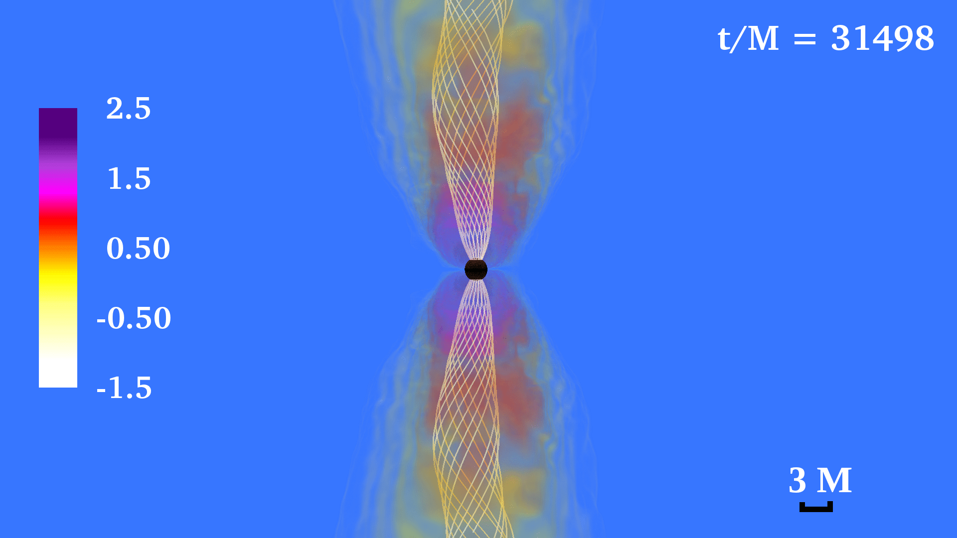
Figure 4: Ratio of magnetic energy density to rest-mass density $b^{2}$/$(8\pi\rho_{0})$ (log scale) at $t-t_{\rm BH}\approx 450M$ for the $\rm S_{\rm{\tiny{Int+Ext}}}$ case. The helical magnetic-field lines (solid curves) are plotted in the collimated funnel with $b^{2}/(8\pi\rho_{0})\geq 10^{-1.5}$. Magnetically dominated areas ($b^{2}/8\pi\rho_{0}\geq 1$) extend to heights greater than $50M\approx 50\,r_{\rm BH}$ above the BH horizon (black sphere).

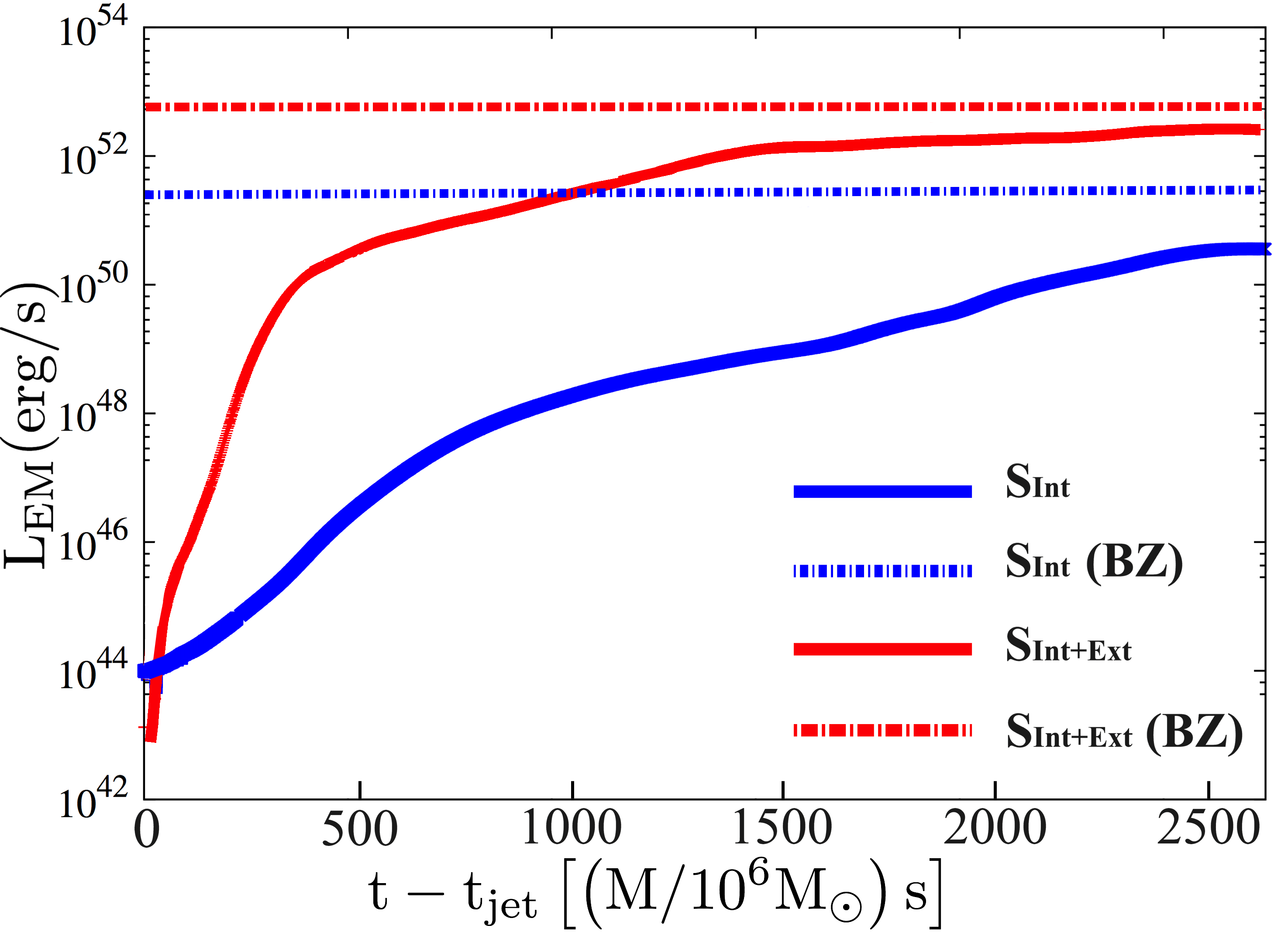
Figure 5: Poynting luminosity $L_{\rm EM}$ vs time $t\geq t_{\rm{jet}}$ calculated on a sphere with coordinate radius $175M=2.43\times 10^{8}(M/10^{6}M_{\odot})\rm km$ for the magnetized cases as displayed in Table 2 (continuous lines). Here $t_{\rm jet}$ defines the time when the jet front reaches 100M above the BH  Ruiz et al. (2016). The dashed part in the $\rm S_{\rm Int+Ext}$ curve indicates the region where the ratio $b^{2}/(2\,\rho_{0})$ becomes $\gtrsim 200$. In that region, our numerical results may not be reliable. The dotted-dashed lines show the expected BZ luminosity computed via Eq. (8) for $M_{\rm BH}$.

To determine if the magnetized outflow is powered by the Blandford-Znajek (BZ) process Blandford and Znajek (1977), we compare the EM luminosity computed via Eq. (7) with the following analytic BZ estimate Blandford and Znajek (1977); Thorne et al. (1986):

$$\begin{multlined}L_{BZ}\approx 10^{51}\left(\frac{a_{\rm BH}/M_{\rm BH}}{0.75}\right)^{2}\,\left(\frac{M_{\rm BH}}{10^{6}M_{\odot}}\right)^{2}\left(\frac{B_{\rm BH}}{10^{10}\text{G}}\right)^{2}\text{erg/s}\,,\end{multlined}L_{BZ}\approx 10^{51}\left(\frac{a_{\rm BH}/M_{\rm BH}}{0.75}\right)^{2}\,\left(\frac{M_{\rm BH}}{10^{6}M_{\odot}}\right)^{2}\left(\frac{B_{\rm BH}}{10^{10}\text{G}}\right)^{2}\text{erg/s}\,,$$ (8)

and show the result in Fig. 5.

Note that in this expression for $B_{\rm BH}$, we use the time-averaged value of the magnetic field that is measured by a normal observer over the last $300M$ before we terminate our simulations. Here $B_{\rm BH}$ scales like $1/M$. Given that $M_{\rm BH}$ scales like $M$, the actual parameter fixed by our simulations is $M_{\rm BH}B_{\rm BH}$: by fixing $\mathcal{M}/|W|$ ($\sim M^{2}B^{2}$ in geometrized units), we fixed the product $MB$. In other words, for our collapse scenario, both the product $M_{\rm BH}B_{\rm BH}$ and hence $L_{BZ}$ are independent of the initial $M$ Shapiro (2017). We find that $L_{\rm EM}~{}\sim 10^{52.5}\rm erg\ s^{-1}$ on an extraction sphere with coordinate radius $175M=2.43\times 10^{8}(M/10^{6}M_{\odot})\rm km$; thus, this is consistent with the BZ process. In addition, we check the ratio of the angular frequency of the magnetic-field lines to the black hole angular frequency, which is expected to be $\Omega_{F}/\Omega_{H}=0.5$ for a split-monopole force-free magnetic-field configuration McKinney and Gammie (2004). Here $\Omega_{F}=F_{t\theta}/F_{\theta\phi}$ is the angular frequency of magnetic field, with $F_{\mu\nu}$ the Faraday tensor, and the angular frequency of the black hole is defined as  Alcubierre (2008)

$$\Omega_{H}=\frac{(a_{\rm BH}/M_{\rm BH})}{2M_{\rm BH}}\,\left(1+\sqrt{1-(a_{\rm BH}/M_{\rm BH})^{2}}\right)\,.$$ (9)

We compute this ratio in magnetically dominated regions on an azimuthal plane passing through the BH centroid and along coordinate semicircles of radii $1.05\,r_{\rm BH}\leq r\leq 1.5r_{\rm BH}$. We find that, within an opening angle of $\theta\sim 20^{\circ}-30^{\circ}$ from the black hole rotation axis, $\Omega_{F}/\Omega_{H}\approx 0.2-0.35$. As it has been pointed out in Paschalidis et al. (2015); Ruiz et al. (2016), the deviation from the value 0.5 could be due to the deviations from strict stationarity and axisymmetry of the spacetime, the non-split-monopole geometry of the magnetic field in our simulations, the gauge used to compute $\Omega_{F}$, and/or insufficient resolution. Despite this discrepancy, the results suggest that the BZ effect is likely operating in our simulations.

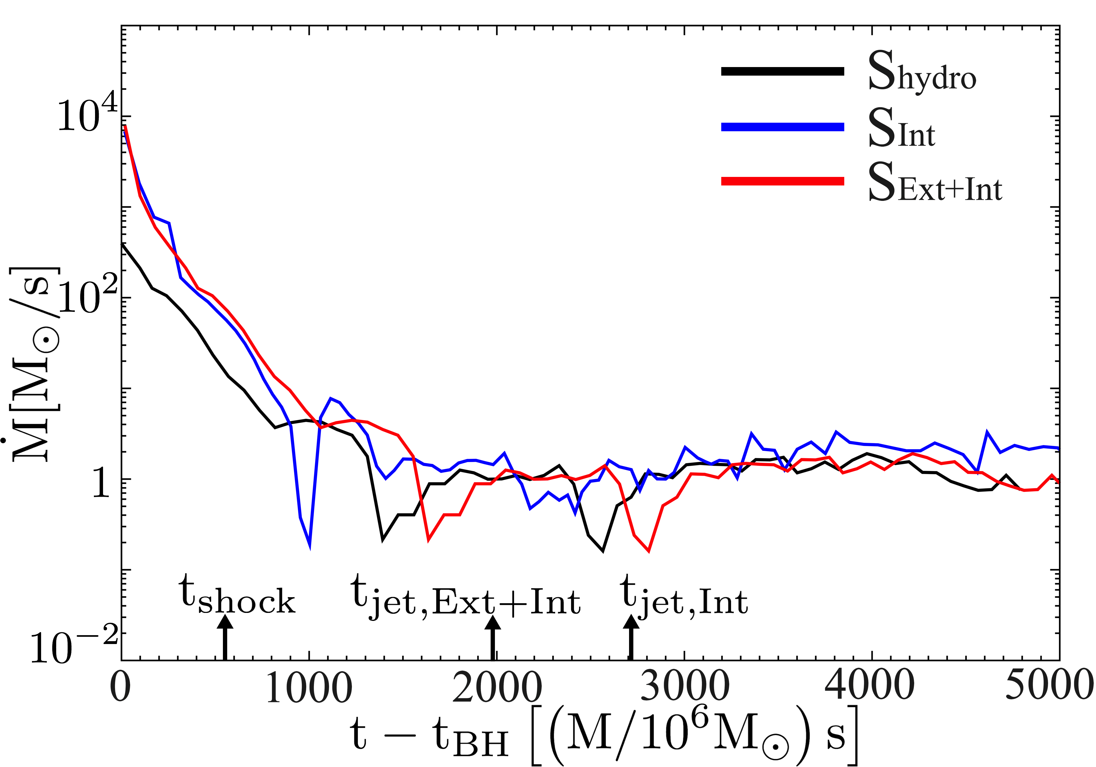
Figure 6: Rest-mass accretion rate $\dot{M}$ for all the cases listed in Table 1. The arrows denote the shock wave formation and the jet launching times, which are defined in the same way as in Paschalidis et al. (2015).

As displayed in Fig 6, the accretion rate settles to $\dot{M}=1.1\,M_{\odot}/$s by $t-t_{\rm BH}\approx 370M=1.8\times 10^{3}(M/10^{6}M_{\odot})$s, at which time the mass of the accretion torus is $M_{\rm disk}=7\times 10^{4}\,M_{\odot}(M/10^{6}M_{\odot})$. Thus, the duration of the jet which is fueled by the torus is expected to last for an accretion time $\Delta t=M_{\rm disk}/\dot{M}\sim 6\times 10^{4}(M/10^{6}M_{\odot})$s, which is consistent with the estimates in Matsumoto et al. (2015). Combining this result with the outgoing Poynting luminosity, we find that the amount of energy anticipated to be removed via electromagnetic processes after an accretion time scale is $\sim 10^{-5}-10^{-3}M$. By contrast, the amount of energy lost in GWs is $E_{\rm GW}\simeq 10^{-6}M$ (see Table 2). Thus, our simulations indicate that collapsing SMSs with mass $\sim 10^{4}-10^{5}M_{\odot}$ are viable jet engines for ultra-long GRBs such as the 25000s-long GRB 111209A Gendre et al. (2013) (though it is not likely that GRB 111209A is related to SMSs since it is observed at a redshift of $z=0.68$), while those with mass larger than $10^{6}M_{\odot}$ do not seem to fit within the GRB phenomenon. On the other hand, our results indicate that collapsing Pop III stars with mass $M\gtrsim 240M_{\odot}$, are viable engines for long GRBs.

IV Observational Prospects

Detection of an EM signal coincident with a GW would mark a “golden moment” in multimessenger astronomy. A simultaneous detection of GW and EM signals with the signatures summarized below would provide direct evidence for the existence of SMSs, and hence provide a major breakthrough in understanding the cosmological formation of SMBHs. In the following section, we discuss the prospects for detecting multimessenger signatures of collapsing SMSs.

IV.1 Gravitational waves

In Fig. 7 we plot the evolution of the real part of the $(l,m)=(2,0)$ mode of $\Psi_{4}$. Given that the collapse proceeds almost axisymmetrically, the $(l,m)=(2,0)$ mode is the dominant one. As the figure demonstrates, there are no significant differences in the waveform among the three cases we consider in this work. The amplitude of $m\neq 0$ modes is smaller than $3\%$ of the $(l,m)=(2,0)$ mode, demonstrating that deviations from nonaxisymmetry remain small throughout the evolution. The oscillation period of the dominant mode after BH formation is $\sim 13M\approx 15.5M_{\rm BH}$, which corresponds to a frequency of $f\approx 15.6(10^{6}M_{\odot}/M)/(1+z){\rm mHz}$. This value is close to the expected quasinormal mode frequency of the $(l,m)=(2,0)$ Kerr mode Berti et al. (2006). We find that our waveforms are in qualitative agreement with the one obtained from axisymmetric GR, purely hydrodynamic simulations of a SMS which is modeled as a $\Gamma=1.335$ polytrope in Shibata et al. (2016c).

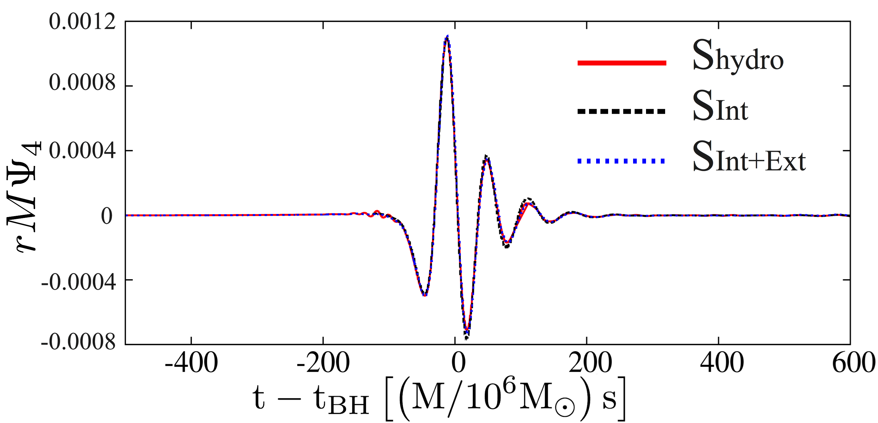
Figure 7: Real part of the $(l,m)=(2,0)$ mode of $\Psi_{4}$ versus time. We have shifted the time in all cases by the coordinate time of black hole formation.

To assess the detectability of GWs produced by SMS collapse, we compute the strain amplitude $|\tilde{h}(f)|=\sqrt{\tilde{h}_{+}(f)^{2}+\tilde{h}_{\times}(f)^{2}}$ from $\Psi_{4}$ and compare it to the expected LISA sensitivity curve eLISA . Here $\tilde{h}_{\times,+}(f)$ are the Fourier transforms of $h_{\times,+}(t)$. The top panel in Fig. 8 shows a plot of twice the characteristic strain $2|\tilde{h}(f)|f$ for all three cases listed in Table 1, assuming $M=10^{6}M_{\odot}$, and cosmological redshift of $z=1$. As expected, all three agree well with each other. We also plot the GW spectra for the S${}_{\text{Int+Ext}}$ case at $z=2$ and $z=3$, assuming $M=10^{6}M_{\odot}$, as well as the LISA noise amplitude $[S(f)f]^{1/2}$ assuming the configuration with four laser links between three satellites, and arm length $L=5\times 10^{6}$km Klein et al. (2016), which has acceleration noise similar to what was found by the LISA Pathfinder experiment Armano (2016). The peak value of the doubled characteristic strain ($h_{2c}=2|\tilde{h}(f)f|$) after taking the $\theta$-averaged value of the ${}_{-2}Y^{2}_{0}$ spherical harmonic is

$$h_{2c}\approx 9.2\times 10^{-21}\left(\frac{M}{10^{6}M_{\odot}}\right)^{-1}\,\left(\frac{6.8\text{Gpc}}{D_{L}}\right)\,.$$ (10)

A source at luminosity distance $D_{L}=6.8$ Gpc lies at redshift $z=1$ in a flat $\Lambda$-CDM cosmology with $H_{0}=67.6\text{km s}^{-1}\text{Mpc}^{-1}$ and $\Omega_{M}=0.311$ Wright (2006); Grieb et al. (2017). Figure. 8 shows that the GW signal frequency lies in the most sensitive part of the LISA sensitivity curve. We compute the signal-to-noise ratio (SNR),

$${\rm SNR}^{2}=\int_{0}^{\infty}\frac{(2|\tilde{h}(f)|)^{2}}{S_{n}(f)}\,df\,,$$ (11)

with $S_{n}(f)$ the one-sided noise spectral density of the detector, and we find that for an optimally oriented source at redshift $z=3$, ${\rm SNR}\sim 7.4$ for the LISA sensitivity curve used in Fig. 8. Thus, if SMSs could form and collapse at redshifts $z\lesssim 3.0$, LISA could detect their GW signature. This is consistent with the axisymmetric simulations of Shibata et al. (2016c).

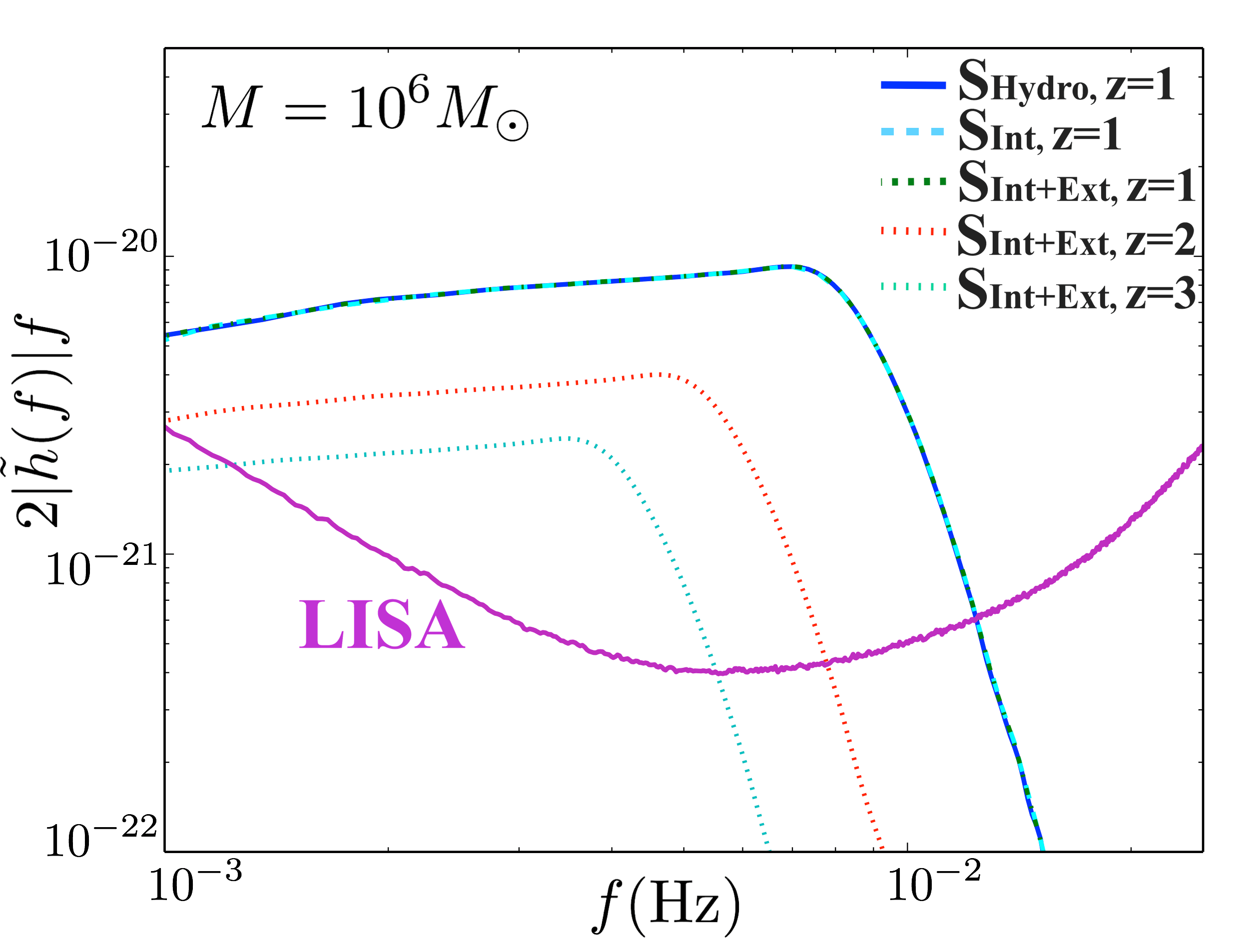
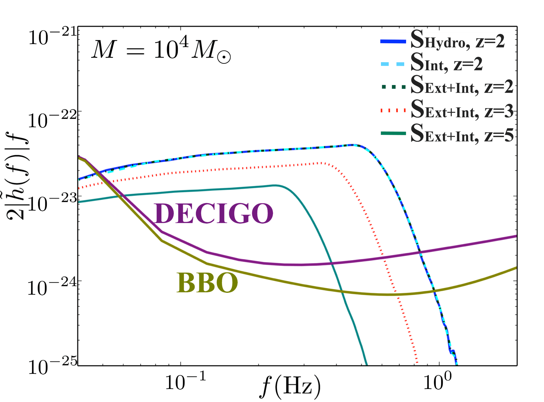
Figure 8: For all of our models, we show $2|\tilde{h}(f)|f$ vs. frequency/ Top panel: The SMS mass is $M=10^{6}M_{\odot}$. The dashed and dotted curves denote the signal strength at redshift $z=1,2$, and 3. The solid curve corresponds to the LISA noise amplitude. Bottom panel: The SMS mass is $M=10^{4}M_{\odot}$. The dashed and dotted curves denote the signal strength at redshift $z=2$, 3, and 5. The solid curves correspond to the DECIGO and BBO noise amplitude as indicated in the plot.

For less massive progenitors ($10^{4}M_{\odot}$), the characteristic strain would peak at the decihertz range. Thus, these sources would be targets for future instruments like BBO  Harry et al. (2006) and DECIGO  Takahashi and Nakamura (2003). Despite the decrease in the amplitude of the GWs due to the lower mass, the superior sensitivity of decihertz GW detectors [$[S(f)f]^{1/2}\sim 10^{-24}$ at $f\sim 0.1$ Hz] makes these systems detectable at very large redshifts. The bottom panel in Fig. 8 shows a plot of the $\theta$-averaged doubled characteristic strain $2|\tilde{h}(f)|f$ for all three cases listed in Table 1, assuming $M=10^{4}M_{\odot}$, and a cosmological redshift of $z=2$. We also plot the GW spectra for the S${}_{\text{Int+Ext}}$ case at $z=3$ and $z=5$, assuming $M=10^{4}M_{\odot}$, and the DECIGO/BBO noise amplitudes based on the analytic fits of  Yagi and Tanaka (2010); Yagi et al. (2011), which account for foreground and background noise sources in addition to the instrument noise. Employing the same detector noise amplitude, we computed the SNR for $M=10^{4}M_{\odot}$, and found that optimally oriented sources could be detected by DECIGO at redshift $z\lesssim 8$ with ${\rm SNR}\gtrsim 8$, and by BBO at $z\lesssim 11$ with ${\rm SNR}\gtrsim 8$. Thus, if the rate of collapsing SMSs at high redshifts is sufficiently high, the exquisite sensitivity of DECIGO/BBO could provide smoking-gun evidence for the existence of such stars and the formation of massive seed BHs.

IV.2 Electromagnetic signatures

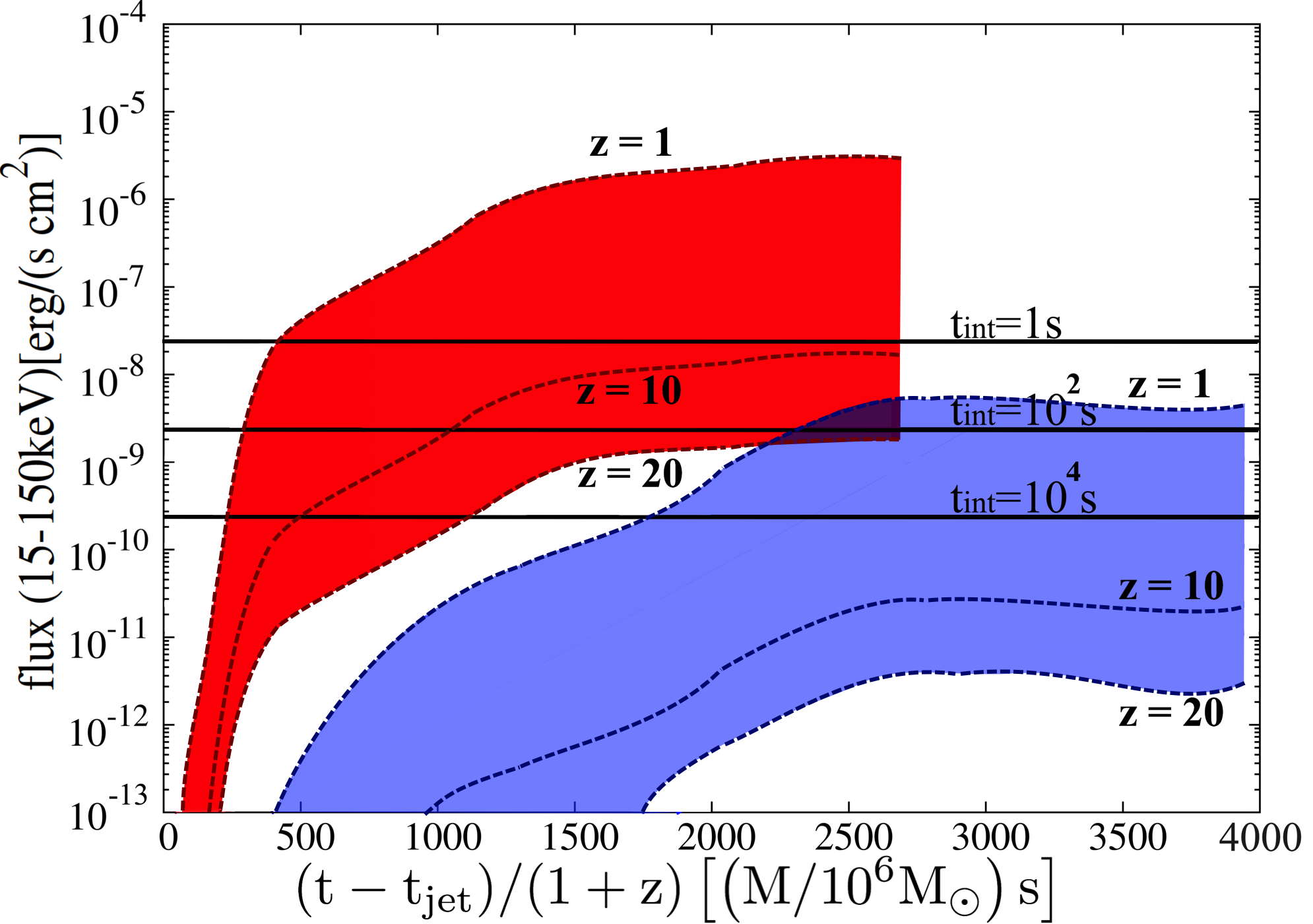
Figure 9: Gamma-ray flux versus time in the energy range $15-150$ keV at different redshifts for the $\rm S_{\rm{\tiny{Int+Ext}}}$ (top-red region) and $\rm S_{\rm{\tiny{Int}}}$ (bottom-blue region) cases. The three horizontal lines show the sensitivity of BAT with integration time of $1$s, $10^{2}$s, and $10^{4}$s, from top to bottom.

To assess the detectability of the EM radiation from our magnetized models by detectors such as the Swift’s BAT, we assume that the following collapse a GRB-like event takes place. We then compute the energy flux within BAT’s energy range (15–150 keV) in the observer frame as follows

$$f=\frac{\epsilon L_{\rm EM}}{2\pi\eta_{c}D^{2}_{L}(z)}\frac{\int^{150(1+z)\text{keV}}_{15(1+z)\text{keV}}EN(E)\text{d}E}{\int^{\infty}_{0}EN(E)\text{d}E},$$ (12)

where $\epsilon$ is the fraction of the Poynting luminosity that becomes photons, $\eta_{c}$ is a “collimation” factor, which equals $2$ for isotropic emission and $0.2$ for a half-opening angle of $25^{\circ}$, $D_{L}(z)$ is the luminosity distance, $N(E)$ is the photon number spectral density in the source frame, and $L_{\rm{EM}}$ is the outgoing Poynting luminosity we compute in our simulations. Photons with energies in the range $15\textendash 150$ keV in the observer frame, originate with energies $15(1+z)\textendash 150(1+z)$ keV in the source frame. Here, we approximate $N(E)$ by the “GRB model” proposed in Band et al. (1993), which consists of a power-law continuum with an exponential cutoff at low energy that continuously transitions to a steeper power law at high energy [see Eq. (1) in  Band et al. (1993)]. In our calculation, the spectral parameters $\alpha$, $\beta$, and $E_{0}$ of Band et al. (1993) are set to -1, -2.3, and 150 keV, respectively Kaneko et al. (2006). In all our estimates in this section, we also choose $\epsilon=0.1$ and $\eta_{c}=0.2$

In Fig. 9 we plot the total energy flux of Eq. (12) as a function of time for sources that are located in the redshift range $1\leq z\leq 20$ and we compare it with BAT’s sensitivity at three different observation periods, $t_{\text{int}}=1,10^{2}$, $10^{4}$s. The luminosity distance is computed assuming the cosmological parameters we listed in the previous section. The detector sensitivities for different observation periods are indicated by the black horizontal lines. We estimate these using the BAT sensitivity derived via a 70-month survey in the 14–195 keV band Baumgartner et al. (2012), and the fact that the sensitivity of BAT approximately increases as $\sqrt{t_{\rm{int}}}$, where $t_{\rm int}$ is the integration or observation time (see, e.g., Ref. Barthelmy et al. (2005)). We find that for the $\rm S_{\rm{\tiny{Int+Ext}}}$ case, up to $z=20$ the EM energy flux is greater than $10^{-10}\text{erg}\text{ /(s}\text{ cm}^{2})$, which BAT is fully capable of detecting with integration time $t_{\rm int}\sim 10^{4}$s. The results also hold approximately for Fermi Gamma-ray Burst Monitor (GBM) whose sensitivity is somewhat smaller than Swift’s  Bosnjak et al. (2014); Connaughton et al. (2013). For the case $\rm S_{\rm{\tiny{Int}}}$, a confident detection can be made up to $z\sim 15$, but it would require integration time $t_{\text{int}}\sim 10^{6}$s, which may be too long. A characteristic-duration ULGRB may be on the order of $10^{4}$s, which would require a disk lifetime of order $10^{3}(1+z)$s in the SMS collapse scenario. Such disk lifetimes could arise for $M\sim 10^{4}M_{\odot}$, for which we estimate that the ULGRB detection could be made even at $z\sim 15$ in the $\rm S_{\rm{\tiny{Int+Ext}}}$ scenario. Consequently, $M\sim 10^{4}M_{\odot}$ SMSs that collapse at $z\sim 10$ are promising candidates for coincident detection of multimessenger EM and GW signals. However, the rates at which such events take place are uncertain and our results motivate their study. Finally, our results suggest that collapsing Pop III stars at redshift $z\sim 5-8$ could be the progenitors of long GRBs that Swift and Fermi could detect. Hence, a fraction of the high-redshift long GRBs that have already been observed could have been powered by collapsing Pop III stars.

V Summary and Conclusions

We performed magnetohydrodynamic simulations in 3+1 dimensions and full general relativity of the magnetorotational collapse of $4/3$ polytropes, spinning initially at the mass-shedding limit and marginally unstable. Our simulations model collapsing SMSs with masses $\gtrsim 10^{4}M_{\odot}$, and they also crudely model collapsing, massive Pop III stars. A major goal of our study was to assess the effects of magnetic fields, and the multimessenger signatures of these astrophysical objects. We extended previous studies by lifting the assumption of axisymmetry and considered magnetic-field geometries that are either completely confined to the stellar interior or extend from the stellar interior out into the exterior. We also considered a purely hydrodynamic case in order to compare with previous GR hydrodynamic simulations of SMS collapse (see, e.g., Refs Shibata and Shapiro (2002); Liu et al. (2007); Uchida et al. (2017)) and followed the post-BH formation evolution for much longer times than previous works. In our magnetized cases we ensured that the initial magnetic field is dynamically unimportant by setting the ratio of the total magnetic to kinetic energy to $0.1$, which corresponds to a magnetic-to-gravitational-binding-energy ratio of $\mathcal{M}/|W|=9\times 10^{-4}$.

In terms of the black hole mass, dimensionless black hole spin and torus mass, the results from our hydrodynamic simulations are consistent with previous semianalytic estimates and axisymmetric simulation in GR reported in Shapiro (2004b); Shibata and Shapiro (2002); Shapiro and Shibata (2002); Liu et al. (2007). We also find that magnetic fields do not affect these global quantities Liu et al. (2007).

In the magnetized cases, following BH formation, we observe the formation of magnetically dominated regions above the black hole poles where the magnetic-field lines have been wound into a collimated helical funnel, within which the plasma flows outwards with a typical Lorentz factor of $\Gamma_{L}\sim 1.2$. This collimated outflow is mildly relativistic, and constitutes an incipient jet. Our analysis suggests that the Blandford-Znajek effect is likely operating in our simulations and could be the process powering these jets. The magnetization $b^{2}/(8\pi\,\rho_{0})$ in the funnel reaches values $\gtrsim 200$, and since for steady-state, axisymmetric jets the magnetization approximately equals the jet terminal Lorenz factor, the jets found in our simulations may reach Lorentz factors $\gtrsim 200$, and hence explain GRB phenomena. The accretion torus lifetime is $\Delta t\sim 10^{5}(1+z)(M/10^{6}M_{\odot})$s. Thus, collapsing supermassive stars with masses $10^{3}-10^{4}M_{\odot}$ at $z\sim 10-20$ are candidates for ultra-long GRBs, while collapsing massive Pop III stars at $z\sim 5-8$ are candidates for long GRBs. We estimated that for observation times $\sim 10^{4}$s, Swift’s BAT and Fermi’s GBM could detect such ultra-long GRB events from $10^{3}-10^{4}M_{\odot}$ supermassive stars at $z\lesssim 15$, and they could also detect long GRB events from Pop III stars at $z\sim 5-8$. While $10^{6}M_{\odot}$ supermassive stars could, in principle, power gamma-rays, our models suggest that the burst duration at $z\sim 10$ would be $10^{6}{\rm s}\sim 114{\rm d}$ long, which would require long integration times to observe.

Apart from sources of EM signals, we also demonstrated that supermassive stars generate copious amounts of gravitational waves with $(l,m)=(2,0)$ the dominant mode, and in agreement with the axisymmetric results of Shibata et al. (2016c). We find that if an optimally oriented $10^{6}M_{\odot}$ SMS collapses to a BH at $z\lesssim 3$, its GW signature could be detectable by a LISA-like detector, with a signal-to-noise ratio $\gtrsim 7.4$. Most importantly, we point out that collapsing supermassive stars with masses $10^{4}M_{\odot}$ generate gravitational waves which peak in the DECIGO/BBO bands, and that BBO (DECIGO) could detect their GWs even at redshifts $z\lesssim 11$ ($z\lesssim 8$). Thus, we discover that $10^{4}M_{\odot}$ supermassive stars are promising candidates for coincident multimessenger signals.

Some comments and caveats about our calculations are in order. First, our numerical results may not continue to be reliable for funnel magnetizations $b^{2}/(8\pi\,\rho_{0})\gtrsim 200$ (see, e.g. Ref. Paschalidis et al. (2015)), which is why we terminate our simulations when such high values are reached. However, based on previous work and tests with our code we are confident that the increase in the magnetization and jet launching is robust. Moreover, by the time we terminate, the BH-disk-jet configuration has settled into quasistationary equilibrium even as the magnetization grows. Second, we used a $\Gamma=4/3$ $\Gamma$-law EOS to model our stars. However, most observed long-gamma-ray bursts are believed to originate from a Pop I star with an EOS that becomes stiffer once the core density approaches nuclear density MacFadyen and Woosley (1999). Third, we have ignored pair-creation effects. Differential rotation may be present in rapidly rotating stars, at least in outer layers Shapiro and Teukolsky (1983). Hence an uniformly rotating model of a supermassive star may only be an approximation. However, differential rotation may not be maintained in turbulent magnetized scenarios Baumgarte and Shapiro (1999). We also neglect the possibility of nuclear burning in the SMS core, although it is unimportant for $M\gtrsim 10^{5}M_{\odot}$ Uchida et al. (2017). We also note that the collapse of differentially rotating supermassive stars with small initial nonaxisymmetric density perturbations may induce the formation of multiple black holes due to a fragmentation instability, as has been reported in pure hydrodynamic studies Zink et al. (2006, 2007); Reisswig et al. (2013). We plan to explore all of these aspects in future investigations.