Effective Field Theory Models for Thermal QCD

Abstract

We present an effective field theory model for QCD at finite temperature with quarks. We discuss the mean field theory, the fixing of parameters, and a prediction for the curvature of the critical line. We proceed to write down a pionic theory of fluctuations around the mean field, and discuss how the parameters of this pionic effective theory descend from the model with quarks.

Nuclear Physics A S. Gupta and R. Sharma nupha Nuclear Physics A

XXVIth International Conference on Ultrarelativistic Nucleus-Nucleus Collisions
(Quark Matter 2017)

1 The effective action

We build the model using the flavour symmetries SU_V($N_{f}$) $\times$ SU_A($N_{f}$), for $N_{f}$ flavours of quarks, acting on Fermion fields which carry Dirac and flavour indices. We also carry along the SU($N_{c}$) colour index, although these contribute only overall factors since there are no colour interactions in the model: every fermion bilinear we use is colour blind. The dimension of the fermion field is ${\cal N}=4N_{c}N_{f}$ where $N_{c}=3$ and $N_{f}=2$. The model is organized by the mass dimension of operators, using an arbitrary temperature scale $T_{0}$ to adjust dimensions if necessary.

We write an Euclidean finite temperature field theory using Hermitean Euclidean Dirac matrices. The Lorentz group becomes a rotation group in Euclidean, with Hermitean generators $S_{\mu\nu}=-i[\gamma_{\mu},\gamma_{\nu}]/4$. The theory breaks the full O(4) rotational symmetry down to a cylidrical symmetry O(3)$\times$Z₂ of spatial rotational symmetry and Euclidean time reversal symmetry T. Every O(4) tensor also reduces, time and space components of 4-vectors transform independently. Our theory then has more couplings than a zero temperature theory.

There is always a possible dimension zero term in any EFT. The coefficient, $d^{0}T_{0}^{4}$, called the vacuum energy, is set to zero. There are no terms of dimension 1 or 2. The only allowed dimension 3 operator $\overline{\psi}{}\psi$ has the quark pole mass as its coefficient, which we write as $m_{0}=d^{3}T^{0}$. The allowed dimension 4 terms are obtained by using derivative operators: $\overline{\psi}{\not{\partial}_{4}}\psi$ and $\overline{\psi}{\not{\partial}}\psi$. Here $\not{\partial}_{4}=\gamma_{4}\partial_{4}$ and $\not{\partial}=\gamma_{i}\partial_{i}$. The coefficient of the kinetic term, $\overline{\psi}{\not{\partial}_{4}}\psi$ fixes the normalization of the field operator, and hence is always set to unity. The coefficient of the other term, $d^{4}$, is special to finite temperature. It relates the pole mass to the quark screening mass. All terms of dimension 5 can be eliminated by symmetry or on using the equations of motion up to dimension 4. Similar arguments resctrict the number of possible dimension 6 terms to ten.

The Euclidean EFT model we start with consists of all possible terms up to mass dimension 6, invariant under the global and space-time symmetries of a finite temperature Euclidean theory,

$$L = d^{3}T_{0}\overline{\psi}{}\psi+\overline{\psi}{\not{\partial}_{4}}\psi+d^{4}\overline{\psi}{\not{\partial}_{i}}\psi+\frac{d^{61}}{T_{0}^{2}}\left[(\overline{\psi}{}\psi)^{2}+(\overline{\psi}{i\gamma_{5}\tau^{a}}\psi)^{2}\right]+\frac{d^{62}}{T_{0}^{2}}\left[(\overline{\psi}{\tau^{a}}\psi)^{2}+(\overline{\psi}{i\gamma_{5}}\psi)^{2}\right]$$

$$+\frac{d^{63}}{T_{0}^{2}}(\overline{\psi}{\gamma_{4}}\psi)^{2}+\frac{d^{64}}{T_{0}^{2}}(\overline{\psi}{i\gamma_{i}}\psi)^{2}+\frac{d^{65}}{T_{0}^{2}}(\overline{\psi}{\gamma_{5}\gamma_{4}}\psi)^{2}+\frac{d^{66}}{T_{0}^{2}}(\overline{\psi}{i\gamma_{5}\gamma_{i}}\psi)^{2}+\frac{d^{67}}{T_{0}^{2}}\left[(\overline{\psi}{\gamma_{4}\tau^{a}}\psi)^{2}+(\overline{\psi}{\gamma_{5}\gamma_{4}\tau^{a}}\psi)^{2}\right]$$

$$+\frac{d^{68}}{T_{0}^{2}}\left[(\overline{\psi}{i\gamma_{i}\tau^{a}}\psi)^{2}+(\overline{\psi}{i\gamma_{5}\gamma_{i}\tau^{a}}\psi)^{2}\right]+\frac{d^{69}}{T_{0}^{2}}\left[(\overline{\psi}{iS_{i4}}\psi)^{2}+(\overline{\psi}{S_{ij}\tau^{a}}\psi)^{2}\right]+\frac{d^{60}}{T_{0}^{2}}\left[(\overline{\psi}{iS_{i4}\tau^{a}}\psi)^{2}+(\overline{\psi}{S_{ij}}\psi)^{2}\right]$$

This differs from the NJL model [1] in two important ways. First, Lorentz invariance is given up since it is built to model QCD at finite temperature, and a temperature scale $T_{0}$ is used to organize the expansion. Second, it is an EFT, so all terms up to a certain order in mass dimension are kept, provided they are invariant under the symmetries of the model. The NJL model would have all four-fermi couplings set to zero except $d^{61}$.

2 The mean field approximation

The mean-field approximation is the fermion operator identity $\overline{\psi}_{\alpha}\psi_{\beta}=\delta_{\alpha\beta}\langle\overline{\psi}\psi\rangle$, where $\alpha$ and $\beta$ are composite Dirac-flavour-colour indices. Performing the Wick-contractions in various ways in the generic 4-fermi term then gives

$$(\overline{\psi}{\Gamma}\psi)^{2}=2\langle\overline{\psi}\psi\rangle\left[{\rm Tr\/}\Gamma\overline{\psi}{\Gamma}\psi-\overline{\psi}{\Gamma\Gamma}\psi\right]-\langle\overline{\psi}\psi\rangle^{2}\left[({\rm Tr\/}\Gamma)^{2}-{\rm Tr\/}(\Gamma\Gamma)\right].$$ (2)

The product of Dirac-flavour matrices in the second term is the Fierz transformation. In this approximation, the EFT becomes

$$L_{{\scriptscriptstyle{\rm MFT}}}=-{\cal N}\left(\frac{T_{0}^{2}}{4\lambda}\right)\Sigma^{2}+\overline{\psi}{\not{\partial}_{4}}\psi+d^{4}\overline{\psi}{\not{\partial}_{i}}\psi+m\overline{\psi}{}\psi$$ (3)

where $\lambda=({\cal N}+2)d^{61}-2d^{62}-d^{63}+d^{64}+d^{65}-d^{66}+d^{69}-d^{60}$, and we define $\Sigma=2\lambda\langle\overline{\psi}\psi\rangle/T_{0}^{2}$, and $m=d^{3}T_{0}+\Sigma$. This is little more than the mean field approximation to the NJL model, so we can utilize the body of work in, for example, [2]. There are several interesting points to note about the sum-integrals required to compute the free energy at finite temperature. After performing the Matsubara sum, one can scale the spatial momenta by $d^{4}$, as a result of which all thermodynamic quantities contain $d^{4}$ as an overall factor. The integral for the free energy density can be written in the form

$$\Omega=\left(\frac{d^{4}}{2\pi}\right)^{3}\int d^{3}p\;\left[TS_{0}(p)+E_{0}(p)+E(p,T)\right].$$ (4)

The temperature independent pieces of the integrand have obvious interpretations; $S_{0}(p)$ is a contribution to the entropy of the vacuum, and $E_{0}(p)$ to its energy. These are formally divergent, and we choose to use dimensional regularization to deal with them. Then the vacuum entropy contribution vanishes and the vacuum energy is regulated. However, this introduces a new scale, $M$, into the problem which can be called the “renormalization scale”. In the chiral limit, $d^{3}=0$, there are two parameters to be determined ($d^{4}$ and $\lambda$) for a given choice of $T_{0}$ and $M$. Due to the scaling of the free energy shown in eq. (4), one cannot use thermodynamic quantities to determine the two parameters independently. Thermodynamics determines only the combination $\lambda/(d^{4})^{3}$.

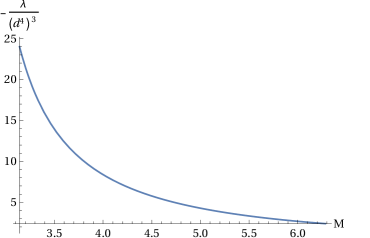
Figure 1: The “running” of the quartic effective coupling as the “renormalization scale” $M$ (given in units of $T_{c}$) is changed in the chiral limit in order to keep $T_{c}$ fixed.

Since we are interested in the low-energy physics around the chiral transition temperature, $T_{c}$, we choose $T_{0}$ to be $T_{c}$. This is an arbitrary choice, and small changes in $T_{0}$ can be compensated by changing the parameters of the Lagrangian, while keeping physical quantities (such as the value of $T_{c}$) unchanged. Similarly, changes in $M$ can be compensated by changes in the parameters. This is the equivalent of renormalization-group flow for the effective model. A typical running of the coupling with the scale is shown in Figure 1. We determine the parameters of the model by taking $T_{c}$ in the chiral limit to be a given value, and using the convention $T_{0}=T_{c}$. It is natural to use a scale $M\simeq$500–700 MeV, between the mass scales of the pseudoscalar and vector mesons. In this case one can choose $\lambda/{\cal N}$ to be attractive and of order one for $T_{c}$ between about 140 Mev and 125 MeV. This is a technically natural value of the coupling.

One interesting parameter-free observable emerges when we introduce a chemical potential through a term $\tilde{\mu}T_{0}\overline{\psi}{\gamma_{4}}\psi$. For small $\mu$ the chiral critical point persists, albeit with a temperature, $T_{c}(\tilde{\mu})$ which shifts with the chemical potential. The curvature of the critical line in the chiral limit is usually given in terms of the expansion $t_{c}(\tilde{\mu})=1-T_{c}(0)\kappa\tilde{\mu}^{2}/2+{\cal O}(\tilde{\mu}^{3})$ where $t_{c}(\tilde{\mu})=T_{c}(\tilde{\mu})/T_{c}(0)$. Estimates of this quantity have been made on the lattice with quarks which are somewhat heavier than found in nature. The lattice results correspond to the range $T_{c}(0)\kappa\simeq 0.01$–0.05.

In the mean-field theory we find the completely parameter-free result

$$t_{c}(\tilde{\mu})=1-\frac{3}{2\pi^{2}}\tilde{\mu}^{2},\qquad{\rm giving}\qquad T_{c}(0)\kappa=\frac{3}{\pi^{2}}.$$ (5)

Although the model prediction in the chiral limit is larger than the lattice determinations, it is not too far away. Since the lattice results are not in the chiral limit, and the model results are in the mean-field approximation, it would be interesting to see how this prediction can be refined.

3 Fluctuations

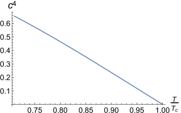
Figure 2: The parameter $c^{4}$ computed by matching the quark effective theory to the pion effective theory in the chiral limit.

The mean-field effective action is invariant under the global vector SU(2) transformations. Local axial SU(2) transformations describe corrections to the mean-field of the kind

$$\overline{\psi}_{\alpha}\psi_{\beta}=\langle\overline{\psi}\psi\rangle U_{\alpha\beta}\qquad{\rm where}\qquad U=\exp\left(\frac{i\tilde{\pi}\gamma_{5}}{f}\right)\times 1,$$ (6)

where $U$ acts in flavour space, and is the identity in Dirac-colour space. The Lagrangian for quadratic fluctuations of coupled to quarks in the mean field approximation is then

$$L=-\frac{{\cal N}}{4\lambda}\Sigma^{2}+\overline{\psi}{\left\{m+\frac{im_{0}\tilde{\pi}\gamma_{5}}{f}-\frac{m_{0}\tilde{\pi}^{2}}{f^{2}}\right\}}\psi+\overline{\psi}{\left\{\not{\partial}-\frac{i}{2f}\gamma_{5}\not{\partial}\tilde{\pi}-\frac{1}{8f^{2}}[\not{\partial}\tilde{\pi},\tilde{\pi}]\right\}}\psi.$$ (7)

The quarks have to integrated out in order to get the effects of the fluctuations. The terms linear in pion fields give tadpole contributions. However, these vanish due to the trace over isospin, $\tau^{a}$. The triangle diagram giving the dimension 3 pion self coupling also vanishes. As a result, the effective action for fluctuations is quadratic

$$L_{f}=\frac{c^{2}T_{0}^{2}}{2}\pi^{2}+\frac{1}{2}(\partial_{0}\pi)^{2}+\frac{c^{4}}{2}(\nabla\pi)^{2}$$ (8)

where the field $\pi=\sqrt{Z_{\pi}}\tilde{\pi}$. $Z_{\pi}$, $c^{4}$ and $c^{2}$ can be computed from eq. (7) by examining two-point function of the pion and then integrating over the quark fields. Such a quadratic theory has been examined earlier [3]. In our approach, this requires constructing an IR effective field theory of pions by matching its parameters to that of the UV effective theory of quarks.

This matching gives us a relation for the effective pion pole mass which is similar to the Gell-Mann-Oakes-Renner relation,

$$c^{2}T_{0}^{2}=-\,\frac{m_{0}\langle\overline{\psi}\psi\rangle}{f^{2}Z_{\pi}}$$ (9)

However, unlike the relation at $T=0$, we have not yet made an identification of $f$ with a measurable scale. So the content of the equation above, as yet, is to define $f$ in terms of other computable quantities. The remaining parameters of the model, namely $c^{4}$ and $Z_{\pi}/f^{2}$ can also be determined.

In the chiral limit we find that $c^{4}$ vanishes linearly as $T\to T_{c}$ (see, for example, Figure 2). As a result, the quadratic theory fails at the critical point, and it is necessary to compute higher order terms in the effective theory in order to obtain critical properties.

Further investigations, including that of the parameters of the effective pion theory away from the chiral limit, are on.

SG would like to acknowledge his J. C. Bose grant number SR/S2/JCB-100/2011.

References

- [1] Y. Nambu and G. Jona-Lasinio, Phys. Rev. 122 (1961) 345; ibid, Phys. Rev. 124 (1961) 246.
- [2] S. P. Klevansky, Rev. Mod. Phys. 64 (1992) 649.
- [3] D. T. Son and M. A. Stephanov, Phys. Rev. Lett. 88 (2002) 202302.