Parallel Multi Channel Convolution
using General Matrix Multiplication

Abstract

Convolutional neural networks (CNNs) have emerged as one of the most successful machine learning technologies for image and video processing. The most computationally-intensive parts of CNNs are the convolutional layers, which convolve multi-channel images with multiple kernels. A common approach to implementing convolutional layers is to expand the image into a column matrix ($im2col$) and perform Multiple Channel Multiple Kernel (MCMK) convolution using an existing parallel General Matrix Multiplication (GEMM) library. This $im2col$ conversion greatly increases the memory footprint of the input matrix and reduces data locality.

In this paper we propose a new approach to MCMK convolution that is based on General Matrix Multiplication (GEMM), but not on $im2col$. Our algorithm eliminates the need for data replication on the input thereby enabling us to apply the convolution kernels on the input images directly. We have implemented several variants of our algorithm on a CPU processor and an embedded ARM processor. On the CPU, our algorithm is faster than $im2col$ in most cases.

I Introduction

Convolutional Neural Networks (CNNs) are one of the most effective machine learning approaches for a variety of important real world problems. CNNs require very large amounts of computation for both training and inference. CNNs are constructed from networks of standard components, such as convolution layers, activation layers and fully-connected layers. In most successful CNNs, the great majority of computation is performed in the convolutional layers.

CNNs require a very large amount of computation, so it is important to make best use of available hardware resources. This hardware may take the form of a standard CPU, or an accelerator such as a graphics processing unit (GPU), digital-signal processor (DSP), or vector architecture. However, making best use of the hardware for computationally intensive problems often requires careful tuning of code to make best use of the memory hierarchy, registers, and vector parallelism. For example, processor/accelerator companies devote very large effort to tuning the performance of standard operators such as those in the the Basic Linear Algebra Subroutines (BLAS) [8].

When implementing CNNs on a new accelerator or processor, it is fortunately possible to exploit existing pre-tuned BLAS routines. In particular, the BLAS general matrix multiplication (General Matrix Multiplication (GEMM)) routine is commonly used to implement DNN convolution. It is well-known that 2D convolution can be implemented using matrix multiplication by converting one of the input matrices to a Toeplitz matrix. This involves replicating image pixels multiple times across different matrix columns. Once the Toeplitz matrix has been constructed, convolution can be implemented using a highly-tuned GEMM for the target architecture.

The $im2col$ approach has been highly successful in Deep Neural Network (DNN) frameworks such as Caffe, Theano and Torch [2]. However, a major downside of $im2col$ is the space explosion caused by building the column matrix. For a convolution with a 2D $k\times k$ kernel matrix, the column matrix is $k^{2}$ times larger than the original image. Deep learning systems are often most useful when deployed in the field, but the space required for the column matrix may be far too large to fit in the memory of an embedded system. Even outside of the embedded context, the increased memory requirement may stretch the limits of on-chip local memories and caches, which may increase execution time and memory traffic.

In this paper we propose a new approach to DNN convolution that allows us to exploit existing optimized routines for accelerators and processors, but does not costly input transformation operations. We make a number of contributions:

• We formulate the problem to operate on a non-replicated input image. This allows us to pose the problem as either one or a sequence of matrix multiplications.

• We present an experimental evaluation of our approach on an embedded processor (ARM® Cortex®-A57), and a general purpose CPU (Intel® Core™ i5-4570) using highly-optimized parallel versions of GEMM.

• Our new GEMM-based approaches perform better than $im2col$ in a great majority of the scenarios tested.

The remainder of this paper is organized as follows. Section II provides additional background and detail on the MCMK convolution operation which is central to deep neural networks. Section III describes how convolution can be implemented with a column matrix. We also show how our proposed approach retains the advantages of re-using GEMM for the computationally-intensive tasks, but with improved data locality. Section IV presents an evaluation of a number of variants of our approach. Finally, Section V describes related work.

II Background

Figure 1: Multiple Channel Multiple Kernel (MCMK) Convolution

In this section, we give an overview of the Convolutional Neural Network (CNN). Traditionally, CNNs are composed of a number of basic building blocks (often referred to as layers): convolutional layer, pooling layer (average and max pooling), activation layer, fully connected layer (FC) and loss layer.

Figure 2: MCMK using the $im2col$ method

II-A Multi-channel convolution as sum of single channel convolutions

In order to understand the core component of a CNN– the convolutional layer, we define dimensions of the inputs, the convolutional kernels (also known as feature maps) and the outputs. A convolutional layer (without batching) takes as input a 3D tensor (input – $\mathcal{I}$) and a 4D tensor (kernel – $\mathcal{K}$) and outputs a 3D tensor (output – $\mathcal{O}$). At the core of any convolutional layer is a Single Channel Single Kernel (SCSK).

Given an input $\mathcal{I}\in\mathbb{R}^{H\times W}$ and a kernel $\mathcal{K}\in\mathbb{R}^{k\times k}$ an output element at position $(x,y)$ where $x\in[0,Q)$ and $y\in[0,P)$, from the output $\mathcal{O}\in\mathbb{R}^{Q\times P}$ is given by

$$conv2D_{x,y}(\mathcal{I},\mathcal{K})=\sum_{i=0}^{i=k-1}\sum_{j=0}^{j=k-1}\mathcal{I}(x-\lfloor\frac{k}{2}\rfloor+i,\\ y-\lfloor\frac{k}{2}\rfloor+j)\times\mathcal{K}(i,j)$$ (1)

where $W$ and $H$ are the width and height of the input; $k$ is the size of the square kernel; $P$ and $Q$ are the width and height of the output which is normally equal to $W$ and $H$ respectively; and assuming the input is properly padded.

The Multiple Channel Single Kernel (MCSK) is then constructed using SCSK, by adding the result of 2D convolutions of the $C$ corresponding channels of the input $\mathcal{I}$ and the kernel $\mathcal{K}$. This is represented as

$$\lx@glossaries@gls@link{acronym}{mcsk}{\leavevmode MCSK}(\mathcal{I}_{C},\mathcal{K}_{C})=\sum_{c=0}^{c=C-1}conv2D(\mathcal{I}(c),\mathcal{K}(c))$$ (2)

where $C$ is the number of channels in the input and kernel and $\mathcal{I}(c)$ and $\mathcal{K}(c)$ represent the $c$^th channel of the input and the kernel respectively. It is imperative to note that the output $\mathcal{O}\in\mathbb{R}^{Q\times P}$ from Equation 1 is a two-dimensional matrix and so is the output of MCSK as shown in 2. As discussed earlier, the convolution layer does MCMK which can expressed as the concatenation of the resultant matrices from Equation 2 as shown in Figure 1 and is represented as

where $\mathcal{K}_{C}^{M}$ represents $M$ kernels with $C$ channels each and the $\mathbin{\|}$ operator denotes the concatenation of two channels.

II-B $im2col$

The $im2col$ approach [1, 11, 13, 3] has been well studied for transforming the MCMK problem into a GEMM problem. Consider an input $\mathcal{I}\in\mathbb{R}^{H\times W\times C}$ and $M$ kernels $\mathcal{K}\in\mathbb{R}^{M\times k\times k\times C}$ as shown in Figure 2. From the input $\mathcal{I}$ we construct a new input-patch-matrix $\hat{\mathcal{I}}$, by copying patches out of the input and unrolling them into columns of this intermediate matrix. These patches are formed in the shape of the kernel (i.e. $k\times k\times C$) at every location in the input where the kernel is to be applied.

Once the input-patch-matrix $\hat{\mathcal{I}}$ is formed, we construct the kernel-patch-matrix $\hat{\mathcal{K}}$ by unrolling each of the $M$ kernels of the shape $k\times k\times C$ into a row of $\hat{\mathcal{K}}$ as shown in Figure 2. Note that this step can be avoided if the kernels are stored in this format to begin with (innermost dimension is the channel which forces the values along a channel to be contiguous). Then we simply perform a GEMM of $\hat{\mathcal{K}}$ and $\hat{\mathcal{I}}$ to get the output $\hat{\mathcal{O}}\in\mathbb{R}^{H\times W\times M}$ as shown in the figure.

It is easy to see from the above discussion how one could implement another method called im2row ($im2row$) wherein the local patches are unrolled into rows of the input-patch-matrix $\hat{\mathcal{I}}$ and the kernels are unrolled into columns of the kernel-patch-matrix $\hat{\mathcal{K}}$. We then perform a GEMM of $\hat{\mathcal{I}}$ and $\hat{\mathcal{K}}$ instead of $\hat{\mathcal{K}}\times\hat{\mathcal{I}}$ as in $im2col$.

ΨΨΨinput[C][H][W];
ΨΨΨkernels[M][K][K][C];
ΨΨΨoutput[M][H][W];
ΨΨΨfor h in 1 to H do
ΨΨΨ for w in 1 to W do
ΨΨΨ  for o in 1 to M do
ΨΨΨ   sum = 0;
ΨΨΨ   for x in 1 to K do
ΨΨΨ    for y in 1 to K do
ΨΨΨ     for i in 1 to C do
ΨΨΨ      sum += input[i][h+y][w+x] *kernels[o][x][y][i];
ΨΨΨ   output[o][w][h] = sum;
ΨΨΨ

Figure 3: Simplified code for 2D multi-channel convolution with a single multi-channel input and multiple multi-channel convolution kernels. Note that special treatment of edge boundaries is not shown in this code.

Figure 4: MCMK using the “$kn2row$” method

III A new approach

A disadvantage of the $im2col$ approach is that it replicates input data to create the input-patch-matrix. For convolution with a $k\times k$ kernel, the input-patch-matrix matrix can be $k^{2}$ larger than the original input. A GEMM-based MCMK algorithm that does not require data replication in the input could be useful for memory-limited embedded systems and might significantly improve data locality on any target architecture. In this section we present two GEMM-based MCMK algorithms that eliminate data replication on the input, at the cost of some increase in the size of the output.

Figure 3 shows a simplified loop nest for $k\times k$ convolution with $M$ kernels each with $C$ channels. A common operation in CNNs such a GoogLeNet [10] is convolution with a set of $1\times 1$ convolutions. If we consider the code in figure 3 for the case where $k=1$, then the $x$ and $y$ loops collapse into a single iteration.

The resulting code is equivalent to 2D matrix multiplication of a $M\times C$ kernel times a $[C]\times[H\times W]$ input which results in a $[M]\times[H\times W]$ output. This output however is actually $M$ planes of $H\times W$ pixels which corresponds to an output of size $[H]\times[W]$ and $M$ channels. Let us call this correspondence of a $[M]\times[H\times W]$ matrix to an output matrix of size $[H]\times[W]$ and $M$ channels its multi-channel representation, which we will use throughout the rest of this section. In other words, $1\times 1$ MCMK can be implemented by simply calling GEMM without data replication.

III-A $kn2row$ and Kernel to Column ($kn2col$)

Given that we can compute $1\times 1$ MCMK without data replication, how can we implement $k\times k$ MCMK, for $k>1$? We argue that a $k\times k$ convolution can be expressed as the sum of $k^{2}$ separate $1\times 1$ convolutions. However the sum is not trivial to compute. Each $1\times 1$ convolution yields a result matrix with dimensions $[M]\times[H\times W]$. We cannot simply add each of the resulting matrices pointwise, as each resultant matrix corresponds to a different kernel value in the $k\times k$ kernel. The addition of these matrices can then be resolved by offsetting every pixel in every channel of the multi-channel representation of these matrices, vertically and/or horizontally (row and column offsets) by one or more positions before the addition.

For example, when computing a $3\times 3$ convolution the result from computing the $1\times 1$ MCMK for the central point of the $3\times 3$ kernel is perfectly aligned with the final sum matrix. On the other hand, the matrix that results from computing the $1\times 1$ MCMK for the upper left value of the $3\times 3$ kernel must be offset up by one place and left by one place (in its multi-channel representation) before being added to the final sum that computes the $3\times 3$ MCMK. Note that when intermediate results of $1\times 1$ convolutions are offset, some values of the offsetted matrix fall outside the boundaries of the final result matrix. These out-of-bounds values are simply discarded when computing the sum of $1\times 1$ convolutions.

It is possible to compute each of the $k^{2}$ separate $1\times 1$ convolutions using a single matrix multiplication. We re-order the kernel matrix, so that the channel data is laid out contiguously, i.e. $M$ is the outer dimension and $C$ the inner. This data re-arrangement can be made statically ahead of time and used for all MCMK invocations thereafter. Using a single call to GEMM, we multiply a $[k^{2}\times M]\times[C]$ kernel matrix by a $[C]\times[H\times W]$ input matrix, resulting in a $[k^{2}\times M]\times[H\times W]$ matrix. We perform a post pass of shift-add by summing each of the $M^{2}$ submatrices of size $M\times[H\times W]$ using appropriate offsetting in the multi-channel representation. The result of this sum is a $[M]\times[H\times W]$ matrix, which is the output of our MCMK algorithm. We refer to this as the $kn2row$ algorithm.

If we swap the dimensions of the kernel matrix so that $C$ is not the innermost dimension and swap the input layout to make $C$ the innermost dimension, we get the $kn2col$ algorithm. The GEMM call in this method would be to multiply an $[H\times W]\times[C]$ input matrix by a $[C]\times[k^{2}\times M]$ kernel matrix, resulting in a $[H\times W]\times[k^{2}\times M]$ matrix.

IV Experiments and Results

We evaluated the proposed MCMK implementations on two general-purpose processors (one embedded, one desktop-class). The experimental platforms we used were ARM® Cortex®-A57 processor, which has 4 cores with a 128-bit wide SIMD unit, and the Intel® Core™ i5-4570, which has 4 cores and a 256-bit wide SIMD unit.

We used GCC version 7.1 to compile our code for the Intel and ARM CPUs. We used the latest stable version (0.2.19) of the high-performance OpenBLAS library to provide the GEMM operation on both ARM and Intel platforms.

We implemented a selection of MCMK operations from three popular CNN architectures: AlexNet [7], VGG-16 [9], and GoogLeNet [10]. In addition to our proposed GEMM based methods, we also implemented a direct convolution to provide some context for performance.

We experimented with several variants of direct convolution, including a version that is used in Caffe [6], and an optimized loop nest that appears in a recent book on optimizing code for the Intel Xeon Phi processor [5]. We found that the fastest direct method, on average, was actually the reference method: summation of single channel convolutions (Equation 2).

We also benchmarked the convolution from Intel’s MKL-DNN framework, which is the backend used by Intel Caffe. MKL-DNN supports AVX2 and AVX-512 processors, and incorporates a code generator which produces highly-optimized SIMD code for convolution.

We found that our GEMM based methods were often much faster than any direct method, and often outperform even the highly-optimized code produced by Intel’s MKL-DNN.

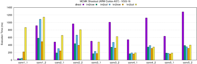
(a) VGG-16

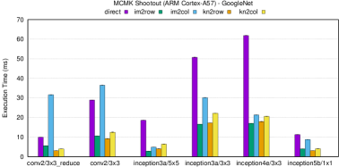
(b) Googlenet

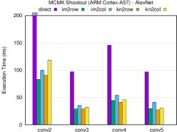
(c) Alexnet

Figure 5: Execution time for selected layers of GoogLeNet, VGG-16 and AlexNet on the ARM® Cortex®-A57 CPU. Lower is better.

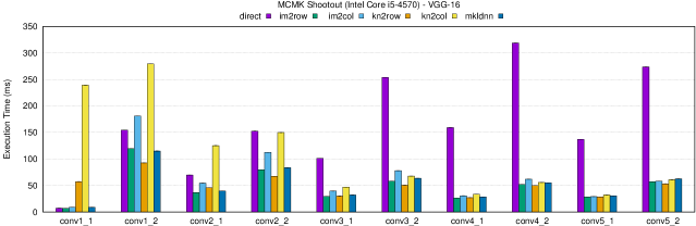
(a) VGG-16

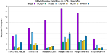
(b) Googlenet

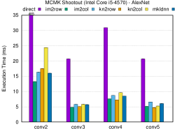
(c) Alexnet

Figure 6: Execution time for selected layers of GoogLeNet, VGG-16 and AlexNet on the Intel® Core™ i5-4570 CPU. Lower is better.

IV-A Performance Trends

Progressing from left to right across each graph in Figures 5 and  6, the number of input channels increases because the operations are drawn from deeper layers of the CNN. At the same time, the size of individual input feature maps diminishes, for the same reason.

Given the fame of $im2col$ in the literature, we were surprised to see that the $im2row$ method performs so well. When data is laid out in a row matrix instead of a column matrix, spatial locality is significantly improved, since consecutive patch elements are consecutive in memory. While the $im2col$ operation may perform well on GPU platforms, our results suggest that it is a poor choice for the implementation of convolution on the CPU.

We also note a large variability between all of the benchmarked methods based on the depth of the convolutional layer in the network. Some methods appear to be very suitable for early layers, but not for later layers; while other methods are unsuitable for early layers, but perform extremely well for later layers. This strongly suggests that a mixture of implementation strategies for convolution is necessary to achieve peak performance.

For example, direct convolution is very performant for first layer of VGG-16, (Figures 5a,  6a) but is quickly outpaced by GEMM based methods as we move deeper in the network. This suggests that peak performance may be achieved by using direct convolution to implement the first layer, and GEMM based convolution for the remaining layers. However, the situation is different for AlexNet (Figures 5c,  6c). Here, the GEMM based methods are always faster.

There is also a similar variability between the GEMM based methods themselves; some GEMM based methods are very suitable for early layers, some are very suitable for late layers, but there is no method that has universally good performance in all contexts.

V Related Work

The $im2col$ method of performing MCMK is an extension of well-known methods of performing 2D convolution using a Toeplitz matrix. Chellapilla et al. [1] are the first researchers to implement MCMK using using $im2col$. They report significant speedups compared to the simpler approach of summing multiple channels of 2D convolutions.

Yanqing et al. rediscovered $im2col$ for the Caffe deep learning system [6], which uses GPUs and other accelerators to speed up DNNs. The $im2col$ approach remains the most widely-used way to implement MCMK, and is used in deep learning frameworks such as Caffe, Theano and Torch.

Gu et al. [4] apply $im2col$ to a batch input images to create a column matrix for multiple input images. They find that batching can improve throughput by better matching the input matrix sizes to the optimal sizes for their GEMM library.

Tsai et al. [12] present a set of configurable OpenCL kernels for MCMK. By coding the MCMK loop nests directly they eliminate the need for $im2col$ data replication, and thus allow the use of larger batch sizes while maintaining constraints on local memory. The found that the performance of a naive loop nest for MCMK is not good, but they achieve satisfactory performance with a program generator and autotuner.

Chetlur et al. [2] propose a GEMM-based approach to convolution based on $im2col$. However, rather than creating the entire column matrix in one piece, they instead lazily create sub-tiles of the column matrix in on-chip memory. To optimize performance, they match the size of their sub-matrix tiles to the tile sizes used by the underlying GEMM implementation. They find that this lazy $im2col$ achieves speedups over Caffe’s standard $im2col$ of between around 0% and 30%.

VI Conclusion

Multi-channel multi-kernel convolution is the most computationally expensive operation in DNNs. Maximal exploitation of accelerator or processor resources for MCMK requires a deep understanding of the micro-architecture. Careful design of data blocking strategies to exploit caches, on-chip memories and register locality are needed, along with careful consideration of data movement and its interaction with SIMD/SIMT parallelism. Each new processor or accelerator has different performance characteristics, requiring careful tuning of the code each time it is brought to a new target.

There are significant advantages in implementing MCMK convolution using existing carefully tuned General Matrix Multiplication (GEMM) libraries. However, the most widely-used approach, $im2col$ has a large memory footprint because it explodes the input image to a much larger column matrix. This space explosion is quadratic in the radix, $k$ of the convolution being performed. This is problematic for memory-constrained systems such as embedded object detection and recognition systems. Additionally, the data redundancy resulting from $im2col$ reduces data locality and increases memory traffic.

We propose new approaches for implementing MCMK convolution using existing parallel GEMM libraries. Our $kn2row$ approach makes one call to GEMM and does a post pass on the output to accumulate the partial results into a single matrix. This drastically increases data locality compared to $im2col$.

Our results strongly motivate the development of a cost model to guide the selection of implementations of MCMK convolution in deep neural networks. The performance of all of the methods which we evaluate is strongly context-dependent, with methods having very good performance in some contexts, and very poor performance in others. The development of this cost model seems a very fruitful avenue for future work in the area.

References

- [1] Kumar Chellapilla, Sidd Puri, and Patrice Simard. High performance convolutional neural networks for document processing. In Tenth International Workshop on Frontiers in Handwriting Recognition. Suvisoft, 2006.
- [2] Sharan Chetlur, Cliff Woolley, Philippe Vandermersch, Jonathan Cohen, John Tran, Bryan Catanzaro, and Evan Shelhamer. cudnn: Efficient primitives for deep learning. CoRR, abs/1410.0759, 2014.
- [3] Junli Gu, Yibing Liu, Yuan Gao, and Maohua Zhu. Opencl caffe: Accelerating and enabling a cross platform machine learning framework. In Proceedings of the 4th International Workshop on OpenCL, page 8. ACM, 2016.
- [4] Junli Gu, Yibing Liu, Yuan Gao, and Maohua Zhu. Opencl caffe: Accelerating and enabling a cross platform machine learning framework. In Proceedings of the 4th International Workshop on OpenCL, IWOCL ’16, pages 8:1–8:5, New York, NY, USA, 2016. ACM.
- [5] James Jeffers, James Reinders, and Avinash Sodani. Intel Xeon Phi Processor High Performance Programming: Knights Landing Edition. Morgan Kaufmann, 2016.
- [6] Yangqing Jia, Evan Shelhamer, Jeff Donahue, Sergey Karayev, Jonathan Long, Ross Girshick, Sergio Guadarrama, and Trevor Darrell. Caffe: Convolutional architecture for fast feature embedding. arXiv preprint arXiv:1408.5093, 2014.
- [7] Alex Krizhevsky, Ilya Sutskever, and Geoffrey E. Hinton. Imagenet classification with deep convolutional neural networks. In Advances in Neural Information Processing Systems, 2012.
- [8] C. L. Lawson, R. J. Hanson, D. R. Kincaid, and F. T. Krogh. Basic linear algebra subprograms for fortran usage. ACM Trans. Math. Softw., 5(3):308–323, September 1979.
- [9] K. Simonyan and A. Zisserman. Very deep convolutional networks for large-scale image recognition. CoRR, abs/1409.1556, 2014.
- [10] Christian Szegedy, Wei Liu, Yangqing Jia, Pierre Sermanet, Scott Reed, Dragomir Anguelov, Dumitru Erhan, Vincent Vanhoucke, and Andrew Rabinovich. Going deeper with convolutions. In Computer Vision and Pattern Recognition (CVPR), 2015.
- [11] Yaohung M Tsai, Piotr Luszczek, Jakub Kurzak, and Jack Dongarra. Performance-portable autotuning of opencl kernels for convolutional layers of deep neural networks. In Proceedings of the Workshop on Machine Learning in High Performance Computing Environments, pages 9–18. IEEE Press, 2016.
- [12] Yaohung M. Tsai, Piotr Luszczek, Jakub Kurzak, and Jack Dongarra. Performance-portable autotuning of opencl kernels for convolutional layers of deep neural networks. In Proceedings of the Workshop on Machine Learning in High Performance Computing Environments, MLHPC ’16, pages 9–18, Piscataway, NJ, USA, 2016. IEEE Press.
- [13] Keiji Yanai, Ryosuke Tanno, and Koichi Okamoto. Efficient mobile implementation of a cnn-based object recognition system. In Proceedings of the 2016 ACM on Multimedia Conference, pages 362–366. ACM, 2016.