Joint Elastic Side-Scattering Lidar and Raman Lidar Measurements of Aerosol Optical Properties in South East Colorado

Abstract

We describe an experiment, located in south-east Colorado, USA, that measured aerosol optical depth profiles using two Lidar techniques. Two independent detectors measured scattered light from a vertical UV laser beam. One detector, located at the laser site, measured light via the inelastic Raman backscattering process. This is a common method used in atmospheric science for measuring aerosol optical depth profiles. The other detector, located approximately 40 km distant, viewed the laser beam from the side. This detector featured a 3.5 m² mirror and measured elastically scattered light in a bistatic Lidar configuration following the method used at the Pierre Auger cosmic ray observatory. The goal of this experiment was to assess and improve methods to measure atmospheric clarity, specifically aerosol optical depth profiles, for cosmic ray UV fluorescence detectors that use the atmosphere as a giant calorimeter. The experiment collected data from September 2010 to July 2011 under varying conditions of aerosol loading. We describe the instruments and techniques and compare the aerosol optical depth profiles measured by the Raman and bistatic Lidar detectors.

1 Introduction

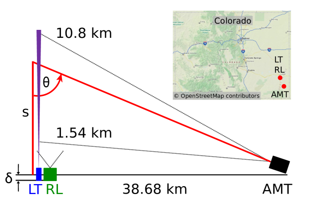
Figure 1: Geometrical arrangement, viewed from the side, of the three instruments used in this experiment. A pulsed UV laser (LT) directed a vertical beam into the atmosphere. Scattered light was measured by the Raman Lidar Detector (RL), and by the Atmospheric Monitoring Telescope (AMT). A map of Colorado [1] showing the location of the instruments is inserted.

Understanding certain properties of the troposphere is critical for ultra high energy cosmic ray observatories that use the atmosphere as an enormous calorimeter. An accurate air density profile is needed to measure the energy deposited in the atmosphere from a cosmic ray extensive air shower (EAS). The amount of UV fluorescence light generated by an EAS is proportional to the energy deposited. The optical clarity of the atmosphere affects the amount of light that reaches the air fluorescence detector (FD) [2]. The latter is the calibration factor with the largest and fastest variation with time.

The most important component of optical clarity is the vertical aerosol optical depth profile, $\tau_{\mathrm{aer}}$. Although usually much smaller in magnitude than the corresponding optical depth profile of the relatively stable molecular component, $\tau_{\mathrm{aer}}$ can vary significantly on the time scale of hours. Under hazy conditions, the apparent brightness of the highest energy EASs can decrease by a factor of 2 or more. Hourly $\tau_{\mathrm{aer}}$ measurements are required. Compounding the measurement challenge is that an FD requires dark, quiet skies to measure EASs effectively. The quiet sky requirement has precluded routine operation of Raman Lidars. To accumulate a statistically significant return profile, many laser pulses (of order $10^{5}$) must be fired into the sky. These pulses will also trigger the FD and cause too much dead time. Still, Raman scattering by N₂ molecules provides a known “atmospheric mirror” that does not depend on the quantity ($\tau_{\mathrm{aer}}$) to be measured. Hence it is the preferred method in atmospheric sciences for measuring aerosol profiles.

To evade the apparent choice between measuring the atmosphere well or measuring the cosmic rays well, the High Resolution Fly’s Eye [3] and the Pierre Auger Observatory [4, 5] adapted an elastic bistatic Lidar technique to measure $\tau_{\mathrm{aer}}$. A UV pulsed laser with optics that aim the beam vertically is operated in the field of view of the FD. The laser wavelength falls near the middle of the EAS UV fluorescence spectrum. As a laser pulse propagates upward through the atmosphere, the elastically scattered light produces a track in the FD which also records tracks of fluorescence light from EASs. The energy of the laser is set to approximate the amount of light observed, under clear conditions, from the very rare highest energy EASs. The laser is placed at a distance from the FD that is typical of the the highest energy EASs observed (10–30 km). With this bistatic technique, the FD provides the receiver and $\tau_{\mathrm{aer}}$ can be measured every 15 minutes with about 200 laser shots per hour.

In this paper we describe an atmospheric research and development program (R&D) that made the first comparison between this elastic bistatic technique and the traditional backscatter Raman Lidar technique. The program was conducted in south-eastern Colorado which is a candidate site for a possible giant cosmic ray observatory. The Raman Lidar receiver developed for this R&D would later be installed at the Pierre Auger Observatory central laser facility [6]. The arrangements of instruments used in the Colorado R&D (Fig. 1) included a frequency-tripled Nd:YAG laser that generated a vertical pulsed beam, a collocated Raman Lidar receiver, and a simplified FD telescope, the Atmospheric Monitoring Telescope (AMT), located about 39 km distant.

This paper is organized as follows. Raman Lidar and side-scattering detector theory is summarized in Sec. 2. Technical details and system performances are presented in Sec. 3. Mode of operations and examples of observations are described in Sec. 4 and  5, respectively. Finally Sec. 6 includes a summary and discussion about future applications of the techniques.

2 Raman LIDAR and Side-Scattering Theory: Measurements of Atmospheric Aerosol Optical Properties

The measurement of atmospheric aerosol optical properties are based on the well-known single scattering Lidar equation and the Raman Lidar principle. In our experiment, the laser has a negligibly small bandwidth of about 1 cm^-1, and the beam is linearly polarized for Raman Lidar (RL) and unpolarized for side-scattering measurements with the AMT. If $L_{0}$ is the number of photons emitted per laser pulse at wavelength $\lambda_{0}$ = 354.7 nm, the number of photons reaching the height $s=ct/2$ (where $c$ is the speed of light, and $t$ the measured time-of-flight of the photons from emission to height $s$ and back to the receiver) above the laser transmitter (LT) is

$$L(s)=L_{0}\cdot T_{\rm aer}(s)\cdot T_{\rm mol}(s),$$

where $T_{\rm aer}(s)$ and $T_{\rm mol}(s)$ are the transmission factors that account for the optical extinction due to aerosol (Mie scattering) and air molecules (Rayleigh scattering),

$$T_{\rm aer}(s) =\exp\left(-\int_{0}^{s}\!\alpha_{\rm aer}(s^{\prime})\,\text{d}s^{\prime}\right),$$

$$T_{\rm mol}(s) =\exp\left(-\int_{0}^{s}\!\alpha_{\rm mol}(s^{\prime})\,\text{d}s^{\prime}\right).$$

$\alpha_{\rm aer}(s)$ and $\alpha_{\rm mol}(s)$ are the aerosol and molecular extinction coefficients,

$$\alpha_{\rm aer}(s) =\int_{0}^{\infty}\!Q_{\rm ext}(r,m,\lambda_{0})\,n_{\rm aer}(s,r)\,\pi r^{2}\,\text{d}r,$$

$$\alpha_{\rm mol}(s) =\sigma_{\rm mol}(s)\cdot n_{\rm mol}(s),$$

where $n_{\rm aer}(s,r)$ is the aerosol size distribution, $Q_{\rm ext}(r,m,\lambda_{0})$ the Mie extinction efficiency of an aerosol particle of radius $r$, and $m$ the index of refraction. $\sigma_{\rm mol}$ is the total Rayleigh scattering cross section at $\lambda_{0}$, and $n_{\rm mol}(s)$ is the number density of air molecules.

A fraction of the $L(s)$ photons is elastically backscattered (scattering angle $\pi$) to the RL by the air molecules and the aerosols,

$$L_{\rm E}(s)=L(s)\cdot\left[\beta_{\rm mol}(s,\pi)+\beta_{\rm aer}(s,\pi)\right]\cdot\Delta s\cdot T_{\rm aer}(s)\cdot T_{\rm mol}(s)\cdot\frac{A_{\rm E}}{s^{2}}\cdot G_{\rm E}(s).$$

These are the detected photons if there is no discrimination of the polarization state. The spectral width of the detector is large enough (i. e., it has the same collection efficiency over a wavelength range of few nanometers centered around $\lambda_{0}$) to detect the unshifted and partly depolarized Cabannes line and the wavelength-shifted and fully depolarized pure rotational Raman lines on both sides of the Cabannes line, coming mainly from the N₂ and O₂ molecules (contributing at a level of about 2% of the total Rayleigh scattering). $A_{\rm E}$ is a constant and is proportional to the area of the RL telescope and the overall detection efficiency of the corresponding Lidar channel, $\Delta s$ is the vertical resolution, which depends on the detector’s electronics. $G_{\rm E}(s)$ is the geometrical overlap function of the elastic Lidar channel, a measure of the height-dependent collecting efficiency of the receiver telescope. It depends on the laser divergence, the receiver field of view and on the distance between telescope and laser axis. $\beta_{\rm mol}(s,\pi)$ is the molecular backscattering coefficient,

$$\beta_{\rm mol}(s,\pi)=\frac{\text{d}\sigma_{\rm mol}(s,\pi)}{\text{d}\Omega}\cdot n_{\rm mol}(s),$$

depending on the local atmospheric molecular number density, $n_{\rm mol}(s)$, and the differential Rayleigh backscattering cross section, $\frac{\text{d}\sigma_{\rm mol}(s,\pi)}{\text{d}\Omega}$, at $\lambda_{0}$. $\beta_{\rm aer}(s,\pi)$ is the aerosol backscatter coefficient,

$$\beta_{\rm aer}(s,\pi)=\int_{0}^{\infty}\!Q_{\rm bck}(r,m,\lambda_{0})\,n_{\rm aer}(s,r)\,\pi r^{2}\,\text{d}r,$$

where $Q_{\rm bck}(r,m,\lambda_{0})$ is the Mie backscatter efficiency.

The Raman-backscattered Lidar return (i. e., by N₂ molecules) for a polarization-independent observation of the complete backscatter signal can be written as

$$L_{\rm R}(s)=L(s)\cdot\left[\beta_{{\rm N}_{2}}^{\rm R}(s,\pi)\right]\cdot\Delta s\cdot T_{\rm aer}^{\rm R}(s)\cdot T_{\rm mol}^{\rm R}(s)\cdot\frac{A_{\rm R}}{s^{2}}\cdot G_{\rm R}(s).$$

The N₂ Raman scattered photons have a shifted (central) wavelength $\lambda_{\rm R}$ of 386.7 nm, if the exciting wavelength is 354.7 nm. The Raman backscatter coefficient at wavelength $\lambda_{\rm R}$, $\beta_{{\rm N}_{2}}^{\rm R}(s,\pi)$, is the product of the differential N₂ Raman backscattering cross section and the molecular number density of the N₂ molecules at height $s$, $n_{{\rm N}_{2}}(s)$,

$$\beta_{{\rm N}_{2}}^{\rm R}(s,\pi)=\frac{\text{d}\sigma_{{\rm N}_{2}}^{\rm R}(\pi)}{\text{d}\Omega}\cdot n_{{\rm N}_{2}}(s).$$

$\text{d}\sigma_{{\rm N}_{2}}^{\rm R}(\pi)/\text{d}\Omega$ is the Raman backscattering differential cross section of the Stokes vibration-rotation Raman lines: the central Q branch and the O and S side-branches that span about 5 nm around the central wavelength. The O and S branches contribute about 14% to the total differential Raman backscattering cross section. $T_{\rm aer}^{\rm R}(s)$ and $T_{\rm mol}^{\rm R}(s)$ are the aerosol and molecular optical transmissions at $\lambda_{\rm R}$, $A_{\rm R}$ is proportional to the area of the RL telescope, and to the detection efficiency of the N₂ Raman Lidar channel. $G_{\rm R}(s)$ is the geometrical overlap function of the Raman Lidar channel. Note that $G_{\rm R}(s)\neq G_{\rm E}(s)$ is possible because, in principle, the field of view of the Lidar receiver can be different for each of the Lidar channels.

A similar equation can be written for the Raman-backscattered Lidar return by water vapor molecules, the H₂O vibration-rotation Raman lines fall at 407.5 nm (Q branch), and the O and S branches (covering an 8 nm interval around the central wavelength) contribute about 9% to the total differential Raman backscattering cross section. The capability of our RL detector of measuring the water vapor content is not reported in this paper, the main reasons are discussed in Sec. 2.1.

$L_{\rm S}(s)$ are the photons side-scattered towards the AMT from a height $s$, the scattering angle is $(\pi-\theta)$ (see Fig. 1)

$$L_{\rm S}(s)=L(s)\cdot\left[\beta_{\rm mol}(s,\pi-\theta)+\beta_{\rm aer}(s,\pi-\theta)\right]\cdot\Delta s\cdot\left[T_{\rm aer}(s)\cdot T_{\rm mol}(s)\right]^{\sec(\theta)}\cdot\frac{A_{\rm S}\cos^{2}(\theta)}{s^{2}},$$

where $A_{\rm S}$ accounts for the aperture and the detection efficiency of the AMT. The scattering coefficients can be written as

$$\beta_{\rm mol}(s,\pi-\theta) =\beta_{\rm mol}(s,\pi)\cdot\frac{P_{\rm mol}(\pi-\theta)}{P_{\rm mol}(\pi)},$$

$$\beta_{\rm aer}(s,\pi-\theta) =\beta_{\rm aer}(s,\pi)\cdot\frac{P_{\rm aer}(\pi-\theta)}{P_{\rm aer}(\pi)}.$$ (2.1)

Here, $P_{\rm mol}(\phi)$ is the Rayleigh scattering phase function, i. e., the probability of a photon being scattered in the direction $\phi$, and $P_{\rm aer}(\phi)$ is the aerosol scattering phase function.

2.1 Raman Lidar

The Raman Lidar is designed to measure the vertical profiles of the aerosol backscatter coefficients $\beta_{\rm aer}(s,\pi)$ and extinction coefficients $\alpha_{\rm aer}(s)$ at the laser wavelength $\lambda_{0}$. The design of the RL receiver includes the capability to detect the H₂O Raman backscattered photons, and with this to measure the water vapor vertical profile. After the first testing phase of the RL, it was found that the liquid light guide (see below) of the receiver shows a fluorescent re-emission when transporting the Lidar backscattered photons, and the fluorescence signal has a spectral signature that directly superimposes the H₂O Raman backscatter signal.

Rayleigh/Mie and Raman Lidar inversion methods for the estimation of the aerosol optical properties are well known, and their combination leads to an improvement of the results [7]. The aerosol extinction can be determined from N₂ Raman Lidar return, through the application of the expression

$$\alpha_{\rm aer}(s)=\frac{\frac{s^{2}L_{\rm R}(s)}{n_{{\rm N}_{2}}(s)}\cdot\frac{\text{d}}{\text{d}s}\left[\frac{n_{{\rm N}_{2}}(s)}{s^{2}L_{\rm R}(s)}\right]-\alpha_{\rm mol}(s)-\alpha_{\rm mol}^{\rm R}(s)}{1+\left(\frac{\lambda_{0}}{\lambda_{\rm R}}\right)^{k}},$$ (2.2)

where $\alpha_{\rm mol}(s)$ and $\alpha_{\rm mol}^{\rm R}(s)$ are the molecular extinctions at $\lambda_{0}$ and $\lambda_{\rm R}$, respectively. $n_{{\rm N}_{2}}(s)$ is the number density of N₂ molecules. The wavelength scaling of aerosol extinction is proportional to $\lambda^{k}$, where $k$ is the Ångstrom coefficient which is in general a function of altitude, since it depends on aerosol properties. A good assumption is to set a value of the Ångstrom coefficient in the interval $k=1.0\pm 0.5$ [8]; this marginally influences the systematic uncertainty affecting the aerosol extinction coefficient, i.e., it introduces an error on the aerosol optical depth less than few percentages. To estimate the aerosol extinction, the derivative of a function containing the Lidar return has to be calculated, represented in discrete range bins. The numerical technique to accomplish this calculation can be the sliding linear least-squares fit. Both $\alpha_{\rm aer}(s)$ and its uncertainty could be misevaluated if data acquisition and analysis are not correctly accomplished.

The uncertainties affecting $\alpha_{\rm aer}(s)$ are the statistical uncertainty due to signal detection, the systematic uncertainty associated with the estimation of the molecular number density and the Rayleigh scattering cross section, the systematic uncertainty associated with the evaluation of the aerosol scattering wavelength dependence (Ångstrom coefficient), and the uncertainties introduced by operational procedures such as signal averaging (accumulating Lidar returns), and by applying, for example, derivative digital filters.

An additional systematic uncertainty that should be accounted for is due to the geometrical overlap function of the Lidar. In a range of heights where the optical overlap between the laser and the field of view of the receiving mirror is range dependent, this uncertainty can be quite important. The atmospheric temperature and pressure profiles from balloon soundings or global meteorological models (i. e., GDAS [9]) are used to estimate the Rayleigh scattering components of the N₂ Raman Lidar return.

Another quantity that is usually evaluated is the vertical aerosol optical depth $\tau_{\mathrm{aer}}$. The $\tau_{\mathrm{aer}}$ profile between the range heights $s_{\rm l}$ and $s$ is defined as

$$\tau_{\rm aer}(s_{\rm l},s)=\int_{s_{\rm l}}^{s}\alpha_{\rm aer}(s^{\prime})\,\text{d}s^{\prime}.$$ (2.3)

Typically, $s_{\rm l}$ coincides with the lower most height at which the N₂ Raman Lidar return is not affected by the optical overlap distortions, the upper limit $s$ is in the free troposphere. Below $s_{\rm l}$ the extinction coefficient is assumed to be a constant $\alpha_{\rm aer}(s_{\rm l})$. The total $\tau_{\mathrm{aer}}$ becomes

$$\tau_{\rm aer}(s)=\alpha_{\rm aer}(s_{\rm l})\cdot s_{\rm l}+\tau_{\rm aer}(s_{\rm l},s).$$ (2.4)

Alternatively, the evaluation of the $\tau_{\mathrm{aer}}$ can be done directly from the N₂ Raman Lidar return,

$$\tau_{\rm aer}(s_{\rm l},s)=-\frac{\log\left(\frac{L_{\rm R}(s)\cdot s^{2}\cdot C}{T_{\rm mol}^{\rm R}(s)\cdot T_{\rm mol}(s)\cdot n_{\rm mol}(s)}\right)}{1+\left(\frac{\lambda_{0}}{\lambda_{\rm R}}\right)^{k}}.$$ (2.5)

The constant $C$ is determined imposing that $\tau_{\mathrm{aer}}$ below $s_{\rm l}$ is a linear function through the origin of the range $s$. Again, this means that the aerosol extinction coefficient is assumed constant in the height range below $s_{\rm l}$.

The aerosol volume backscattering coefficient is evaluated starting from the ratio between the elastic and Raman Lidar returns,

$$\beta_{\rm aer}(s)=\beta_{\rm mol}(s)\cdot\left[0.781\cdot\frac{L_{\rm E}(s)}{L_{\rm R}(s)}\cdot\frac{A_{\rm R}\cdot G_{\rm R}(s)}{A_{\rm E}\cdot G_{\rm E}(s)}\cdot\frac{\frac{\text{d}\sigma_{\rm N_{2}}^{\rm R}(\pi)}{\text{d}\Omega}}{\frac{\text{d}\sigma_{\rm mol}(s,\pi)}{\text{d}\Omega}}\cdot\frac{T_{\rm mol}^{\rm R}(s)\,T_{\rm aer}^{\rm R}(s)}{T_{\rm mol}(s)\,T_{\rm aer}(s)}-1\right]$$ (2.6)

The design of our Raman Lidar receiver (the telescope is coupled to the detector box through a liquid light guide) assigns the same optical overlap modulation to the Rayleigh/Mie elastic and inelastic N₂ Raman Lidar channels. Since the evaluation of $\beta^{\lambda_{0}}_{\rm aer}(s)$ involves the ratio between these two Lidar returns, the estimation of the aerosol backscattering coefficient results are independent of the Lidar geometrical overlap, assuming $G_{\rm R}(s)=G_{\rm E}(s)$. After the estimation and the removal of the Rayleigh scattering and backscattering contributions and of the aerosol transmission as evaluated from the aerosol extinction, a calibration is needed. In other words, the quantity

$$\frac{A_{\rm R}}{A_{\rm E}}\cdot\frac{\frac{\text{d}\sigma_{\rm N_{2}}^{\rm R}(\pi)}{\text{d}\Omega}}{\frac{\text{d}\sigma_{\rm mol}(s,\pi)}{\text{d}\Omega}}$$ (2.7)

has to be estimated. Usually this is done by imposing $\beta^{\lambda_{0}}_{\rm aer}(s)=0$ in a range of altitudes free of aerosols, i. e., in the upper troposphere [10].

The uncertainties affecting $\beta^{\lambda_{0}}_{\rm aer}(s)$ are mainly due to the statistical uncertainty in the signal detection, the systematic uncertainty associated with the estimation of the molecular number density (i. e., from pressure and temperature vertical profiles) and the Rayleigh scattering cross section, and the uncertainties introduced by operational (retrieval) procedures, as the estimation of the quantity in equation (2.7).

2.2 Side-scattering experiment

The AMT is designed to measure $\tau_{\mathrm{aer}}$ directly. The method relies on the assumption that during a measurement as close in time as possible to the actual sampling of the atmosphere $L_{\rm S}(s)$, conditions can be found in which the atmosphere can be considered free of aerosols. In this case the side-scattering return can be expressed as

$$L_{\rm S}^{\rm clean}(s)=L_{0}\cdot T_{\rm mol}(s)\cdot\left[\beta_{\rm mol}(s,\pi-\theta)\right]\cdot\Delta s\cdot\left[T_{\rm mol}(s)\right]^{\sec(\theta)}\cdot\frac{A_{\rm S}\cos^{2}(\theta)}{s^{2}}.$$

The ratio between $L_{\rm S}(s)$ and $L_{\rm S}^{\rm clean}(s)$ is

$$\frac{L_{\rm S}(s)}{L_{\rm S}^{\rm clean}(s)}=\left[T_{\rm aer}(s)\right]^{1+\sec(\theta)}\cdot\frac{\left[\beta_{\rm mol}(s,\pi-\theta)+\beta_{\rm aer}(s,\pi-\theta)\right]}{\left[\beta_{\rm mol}(s,\pi-\theta)\right]}.$$

Recalling Eq. (2), considering that in our configuration $\theta\in\left[74.8^{\circ},87.8^{\circ}\right]$, and that for most of the atmospheric aerosol the scattering phase function is peaked in forward and backward directions, it can be assumed that [11]

$$P_{\rm aer}(\pi-\theta)\ll P_{\rm aer}(\pi).$$

Because the laser light is unpolarized and $\frac{P_{\rm mol}(\pi-\theta)}{P_{\rm mol}(\pi)}\gtrsim 0.5$,

$$\beta_{\rm mol}(s,\pi-\theta)\gg\beta_{\rm aer}(s,\pi-\theta).$$

Finally, $\tau_{\mathrm{aer}}$ can be written as

$$\tau_{\rm aer}(s)=-\frac{1}{1+\sec(\theta)}\cdot\log\left[\frac{L_{\rm S}(s)}{L_{\rm S}^{\rm clean}(s)}\right]$$ (2.8)

The errors on $\tau_{\mathrm{aer}}$ are mainly due to the relative calibration of the AMT, the relative uncertainty in the determination of the $L_{\rm S}^{\rm clean}(s)$, and the statistical fluctuations introduced by signal averaging.

3 Description and Performances of the Instruments

The main criteria that define the constraints of our experimental setup are

• nighttime measurements in new and crescent moon phases,

• high accuracy measurements of aerosol optical properties in the planetary boundary layer and in the lower troposphere,

• remote operations and minimal maintenance.

The laser transmitter system (LT), collocated Raman Lidar (RL) detector and distant side-scattering detector called Atmospheric Monitoring Telescope (AMT) comprise the experiment (Fig. 1). The LT and RL point vertically. The optical axis of the AMT is pointed above the LT, the field of view extends from 2.2^∘ to 15.2^∘. The corresponding sampling heights at the LT location range from 1.5 km to 10.6 km above ground level. The LT and RL are located at 37.9228^∘ N, 102.6109^∘ W and 1198 m a.s.l. in Prowers County, Colorado, about 15 km south of Lamar. The AMT is located at 37.6010^∘ N, 102.4420^∘ W, 1279 m a.s.l. close to the town of Two Buttes in Baca County, Colorado. The sites are 38.7 km apart. The difference in altitude between the two sites $\delta$ is 81 m, this difference as well as the curvature of the Earth are taken into account in the data analysis. In the azimuth direction, the AMT points 337.52^∘ clockwise from north.

3.1 The Laser Transmitter

The optics of this system (Tab. 1) were arranged as shown in Fig. 2. Dichroic beam splitting mirrors (DBS) removed the residuals of the primary and secondary harmonics. A motorized flipper mirror (FM) was raised or lowered to switch between two beam paths. The LT Raman path (LTR) was used to direct pulses at 100 Hz into the sky for RL measurements. The LT side scatter path (LTS) included a depolarizer (DP) and a pick-off energy monitor. This path was used to direct pulses vertically at 4 Hz for measurements by the AMT. The properties of the two beams delivered to the sky are listed in Tab. 1. Although a single beam path could have been used in theory, in practice the use of separate paths simplified the operation and alignment procedures considerably without compromising the scientific objectives. The LTR beam direction was fine tuned to match the direction of the optical axis of the RL mirror (which pointed in the nominal vertical direction). Independently, the direction of the other path was set to vertical relative to a laser level alignment device that was also used in the alignment of the AMT.

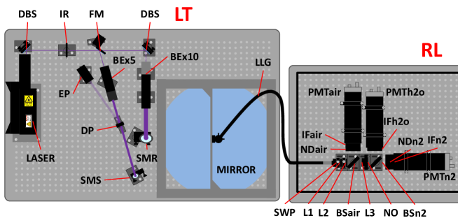
Figure 2: The laser transmitter and the Raman Lidar receiver layout (top view), ND_air and ND_N₂ are combinations of neutral density filters (see text).

Table 1: Technical specification of the Laser Transmitter subsystem.

Laser	Big Sky Laser Centurion Nd:YAG
Wavelength	354.7 nm
Line width	$\sim$ 1 cm-1
Spectral Purity	$>$ 99$\%$
Pulse duration	7 ns
Output energy	6 mJ (nominal)
Divergence LTR/LTS	0.3 mrad/0.6 mrad
Polarization LTR/LTS	linear/randomized
Rep. Rate LTR/LTS	100 Hz/4 Hz
1′′ dichroic beam splitter (DBS)	CVI BSR-35-1025
Flipper mirror (FM)	Newport 8892-K and CVI BSR-31-1025
5x beam expander (BEx5)	CVI BXUV-10.0-5X-354.7
10x beam expander (BEx10)	Thorlabs ELU-25-10X-351
2′′ steering mirror (SMR)	Newport 20QM20EN.35
1′′ steering mirror (SMS)	CVI BSR-35-1025
Depolarizer (achromatic) (DP)	Thorlabs DPU-25-A

3.2 Raman Lidar

The receiving telescope of the Raman Lidar consists of a 50 cm diameter $f/3$ parabolic mirror pointing vertically beneath a UV transmitting silica window and a motorized roof hatch. A liquid light guide couples the light reflected from the mirror to a three-channel receiver. Dichroic beam splitters direct this light onto three photomultiplier tubes (PMTs) that are located behind narrow-band optical filters. These isolate the three scattered wavelengths of interest, 354.7 nm (Rayleigh/Mie or elastic scattering), 386.7 nm (Raman N₂ backscattering), and 407.5 nm (Raman H₂O backscattering). The data acquisition system uses analog (up to 80 MHz A/D) and photon counting (maximum count rate 250 MHz) acquisition modules. The LT and RL are located in a temperature conditioned building, rain and wind sensors conditionally control the opening and closing of the roof hatch, see Sec. 3.3.5.

The RL receiver collects the fraction of the laser beam photons that are backscattered by the elastic Rayleigh and Mie scattering processes, as well as those photons that are inelastically backscattered by N₂ and H₂O Raman scattering processes. A scheme of the receiver can be found in Fig. 2. It consists of a parabolic mirror, a liquid light guide (LLG) that transports the collected light into the detector box containing a combination of dichroic beam splitters (BS), interference filters (IF), neutral density filters (ND), a notch filter (NO), three field lenses (L1, L2, L3) that are combined to collimate the light beam, and the detectors (PMTs). The optical and spectral characteristics of the different components can be found in Tab. 2 and Tab. 3, respectively. The read out of the PMTs is carried out by electronic acquisition cards based on FPGA technology. These low-consumption and low-cost cards simultaneously record the signals in current mode (A/D) and photon counting mode (PhC). Electronic specifications are listed in Tab. 4. Details of the RL performance are discussed in the next three subsections.

Table 2: Technical specification of the Raman Lidar receiver optics.

Telescope	Marcon parabolic mirror
Diameter	504 mm
Focal length	1500 mm
Coating	MgF2 and Al protection
Surface quality	$\lambda/8$ RMS
Liquid light guide (LLG)	Newport 77629
Light collimator (L1, L2, L3)	Thorlabs lenses LA1951/LA1131/LA1986
Effective focal length at 354.7 nm	$\simeq$ 165 mm

Table 3: Technical specification of the spectral features of the Raman Lidar receiver.

Air beam splitter (BS_air)	Barr BS-R345-361nm
Reflectance at 354.7 nm	$\geq$ 99%
N2 beam splitter (BS_N2)	Barr BS-R407-T320-395nm
Reflectance at 407.5 nm	$\geq$ 99%
Air interference filter (IF_air)	Barr IF-CWL354.7-BW6nm
Central wavelength and bandwidth	354.7 nm and 6 nm
Transmittance at 354.7 nm	$\geq$ 83%
N2 interference filter (IF_N2)	Barr IF-CWL3867-BW10A
Central wavelength and bandwidth	386.7 nm and 1 nm
Transmittance at 386.7 nm	$\geq$ 77%
H2O interference filter (IF_H2O)	Barr IF-CWL4075-BW10A
Central wavelength and bandwidth	407.5 nm and 1 nm
Transmittance at 407.5 nm	$\geq$ 65%
Notch filter (NO)	Barr LWP-T-378/415nm
Rejection at 354.7 nm	Optical density $\geq$ 6
Short wavelength pass filter (SWP)	Newport 10-SWP-500

Table 4: Technical specification of the Raman Lidar receiver detectors.

2′′ Photomultipliers (PMT)	Electron Tubes 9828B
Typical quantum efficiency	35%
Gain	2.5 $\times$ 106
Single electron rise time	2 ns
DAQ cards	Embedded Devices APC-80250DSP
Channels	2, analog (A/D) and photon counting (PhC)
Single photon maximum count rate	250 MHz
PhC bin temporal resolution	between 100 and 1000 ns
PhC dead time between channels	$<$ 1 ns
A/D acquisition	up to 80 MHz
A/D bandwidth	20 MHz
A/D resolution	12 bit

3.2.1 Optical Efficiency

The LLG input end is centered on the parabolic mirror axis, in a position close to the focal plane. In this configuration the telescope has a field of view (half angle) of about 2.7 mrad. The LLG output connects to the detector box, where the transported light is directed by a combination of lenses onto the dichroic beam splitters and the optical filters that separate the different Lidar returns according to the wavelength. The RL receiver has been simulated with the Zemax® optical design program, assuming that the pointing direction of the laser beam is perfectly aligned with the telescope axis. The design parameters considered in the simulation are:

• the laser divergence (0.3 mrad half angle);

• the distance between the laser beam and the telescope axes (about 310 mm);

• obscuration effects of the telescope frame and of the LLG holder;

• an estimation of the refractive indexes of the LLG core and cladding materials;

• the length and core dimension of the LLG;

• the distance of the LLG input end above the infinity focus position of the parabolic mirror;

• the optical characteristics and the relative position of the lenses, dichroic beam splitters and optical (interference, neutral and notch) filters.

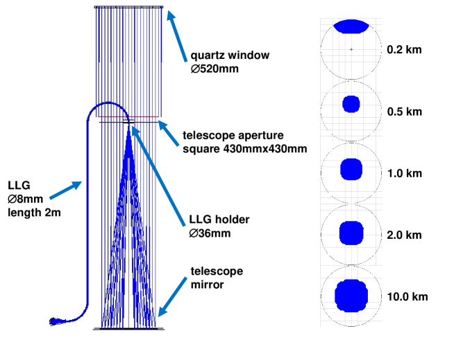
Figure 3: Simulation of receiver telescope and LLG. Left: Layout of part of the simulation. Right: Laser beam image at the LLG input as a function of the distance from the telescope. The LLG input is positioned +9.0 mm above the infinity focus position of the parabolic mirror.

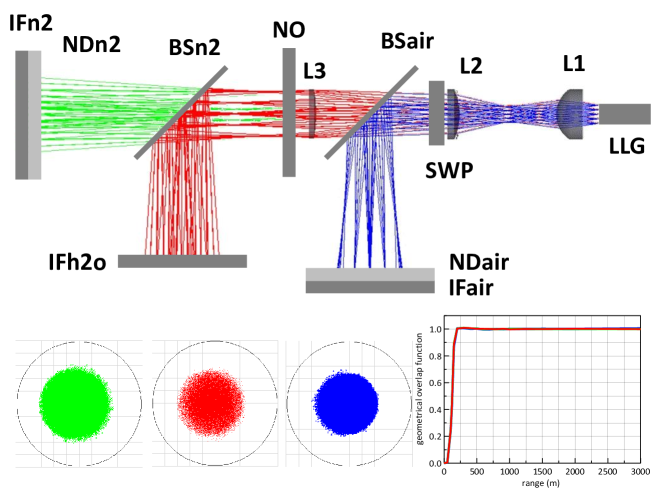
Figure 4: Simulation of RL detector box. Top: Ray tracing simulation of the detector box. Bottom: Dimension of the light spots at wavelengths 354.7, 386.7 and 407.5 nm over the interference filters. In the lower right corner, the coincident geometrical overlap functions for the different RL detection channels are shown.

The layout of part of the simulation is shown in the left panel of Fig. 3. The silica window, the telescope and LLG frames, and the parabolic mirror, as well as the LLG can be represented in the simulation with the real dimensions. The ray tracing calculation allows one to estimate the optical efficiency of the system in collecting the Lidar returns from different heights. The distance of the LLG input end above the infinity focus position of the parabolic mirror is one of the parameters that can be optimized to improve the optical efficiency of the RL receiver, i. e., the geometrical overlap function. In the right panel of Fig. 3, the laser beam image at the LLG input as a function of the distance from the telescope is shown for an LLG input position of +9.0 mm above the infinity focus position of the parabolic mirror. In this position, the geometrical collecting efficiency is full (i. e., the entire image is transmitted into the LLG) from the lowest range of about 300 m. Upper and lower positions of the LLG end determine worse overlap functions (i. e., full overlap at higher heights or a decrease in the collection efficiency of light from higher altitudes). The laser beam image on LLG has a maximum diameter $\leq$ 5.0 mm and the impinging rays have an incident direction that spreads over a numerical aperture (NA) of $\sim$ 0.16. The propagation of the light (at 354.7, 386.7 and 407.5 nm) along the LLG preserves the NA. At the exit of the LLG, the light rays are distributed over the entire LLG end diameter of 8 mm, with exiting directions within an NA of $\sim$ 0.15.

The ray tracing simulation of the detector box is illustrated by the optical layout in upper part of Fig. 4. In the lower part, the dimension of the light spots at the different wavelengths over the interference filters are shown. The 354.7 nm light on the air interference filter (IF_air) falls within a circle of diameter $\sim$ 15.5 mm, with an angle of incidence that is $\in\left[0^{\circ},6^{\circ}\right]$. The N₂ Raman backscattered photons on the N₂ interference filter (IF_N₂) are diffused over a circle of $\sim$ 17.0 mm diameter, and the maximum angle of incidence is $\sim$ 3.5^∘. For H₂O Raman backscattered photons the diameter of the beam and maximum incident angle over the interference filter (IF_H₂O) are $\sim$ 16.5 mm and $\sim$ 3.5^∘, respectively. For such values of the beam dimensions there are no important effects related to the spectral characteristics of the dichroic beam splitters and interference filters. Moreover, the light beams propagating into the RL detector box are slightly diverging/converging by less than 6^∘ off the normal incidence on the interference filters. This causes only a small decrease of less than 0.1% of the central wavelength of the IFs. The decrease of the transmittance and the increase of the bandwidth of the IFs are negligible [12].

Finally, in the lower right corner of Fig. 4, the relative geometrical overlap functions for all Lidar channels as evaluated in the simulation are shown. They are coincident, and the full overlap is achieved just above a range of 250 m.

3.2.2 Spectral Features

The atmospheric backscatter spectrum for an incident laser wavelength of 354.7 nm is determined by the Rayleigh, Mie and Raman scattering processes. For air at pressure $P$ = 101 325 Pa, temperature $T$ = 300 K, a relative N₂ abundance of 0.781, and a content of water vapor of 10 g kg^-1 of air, the Rayleigh backscattered photons in general have a wavelength coincident with the one of the incident photons (Cabannes line), but they also include photons backscattered by pure rotational Raman scattering process of atmospheric nitrogen, oxygen and other molecules. It has to be mentioned that in the presence of atmospheric aerosols, their contribution (Mie scattering) superimposes to the Rayleigh backscattered light and has a narrower spectral width. About 98% of Rayleigh backscattered photons are in the Cabannes line that has a spectral width coincident with that of the laser line. The other photons have wavelengths that cover a band of few nanometers ($\pm$ 3 nm) centered around 354.7 nm. The Stokes vibration-rotation Raman backscattering of the N₂ and H₂O molecules produce photons that have wavelengths around 386.7 nm and 407.5 nm, respectively. For N₂ Raman backscattering, $\sim$ 86% of the energy is at 386.7 nm (Q branch), and the rest is in the O and S side branches that span about 5 nm around the central line; the complete H₂O Raman backscattering is in 407.5 $\pm$ 3 nm [13, 14].

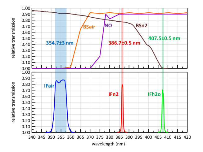
Figure 5: The spectral characteristics of the dichroic beam splitters (BS), the notch filter (NO), and of the interference filters (IF). The blue, red and green bands indicate the FWHH of the various IFs.

The relative spectral transmissivities of the dichroic beam splitters, notch and interference filters combined in the RL detector box are shown in Fig. 5. The blue, red and green bands represent the FWHH (6.0 nm, 1.0 nm and 1.2 nm for IF_air, IF_N₂ and IF_H₂O) of the transmission curves of the interference filters (bottom panel). The BSs separate the different wavelengths in a quite efficient way (i. e., BS_air reflects $\sim$ 99.8% of 354.7 nm and transmits $\sim$ 91.4% and $\sim$ 91.7% of 386.7 and 407.5 nm photons). The NO prevents the propagation of elastic photons in the Raman detection channels (the NO optical rejection ratio at 354.7 nm is $\sim$ 1:10⁶, and the transmissivity at 386.7 and 407.5 nm is $\sim$ 90.0%). The FWHH of the interference filters mainly determine how much of the Rayleigh/Mie, N₂ and H₂O Raman backscatter spectrum is collected by the corresponding Lidar channels: CH_air, CH_N₂ and CH_H₂O. The convolution of the relative spectral transmissions of the IFs with the Rayleigh/Mie and Raman bands gives:

• CH_air collects $\sim$ 99% of the total Rayleigh/Mie backscatter spectrum,

• CH_N₂ collects $\sim$ 95% of the total N₂ Raman backscatter spectrum,

• CH_H₂O collects $\sim$ 99% of the total H₂O Raman backscatter spectrum.

The individual line strengths in the Raman spectra are temperature dependent [15]. In principle, the collected Lidar backscatter returns may be temperature sensitive, especially when only a portion of them is detected. In our case, the percentage changes in the detected energy, backscattered by the atmospheric medium with temperatures from 200 to 300 K (the typical range of temperature in the troposphere) is less than a few tenths of a percent for the Rayleigh and Raman bands: our system has a detection capability that is temperature insensitive.

The ratios between the Raman backscatter coefficients of N₂ and H₂O molecules and the Rayleigh backscatter coefficient are $\sim$ 7.1 $\times$ 10^-4 and $\sim$ 3.4 $\times$ 10^-5, respectively. The spectral discrimination of the different RL detection channels has to be quite efficient to avoid cross-talk effects (i. e., the propagation of elastically backscattered photons in the CH_N₂ and CH_H₂O). The combination of the dichroic beam splitters with the notch and interference filters (see Fig. 5) determines the total spectral collection efficiency $\eta_{ij}$ of the different Lidar returns ($i$ = 354.7, 386.7 and 407.5 nm) in the RL channels ($j$ = CH_air, CH_N₂ and CH_H₂O). $\eta_{ij}$ includes also the spectral reflectivity of the telescope, the transmissivities of light guide, lenses, beam splitters, interference filters, etc.. The values of $\eta_{ij}$ for the three channels and wavelengths are listed in Tab. 5.

Table 5: $\eta_{ij}$ for the three receiver channels at each of the three wavelengths.

$\eta_{ij}$	CH_air	CH_N2	CH_H2O
354.7 nm	$\sim 3.7\times 10^{-6}$	$\sim 4.0\times 10^{-21}$	$\sim 1.3\times 10^{-21}$
386.7 nm	$\sim 1.3\times 10^{-12}$	$\sim 1.3\times 10^{-2}$	$\sim 1.5\times 10^{-6}$
407.5 nm	$\sim 1.6\times 10^{-12}$	$\sim 1.4\times 10^{-8}$	$\sim 3.7\times 10^{-2}$

The Rayleigh and Raman backscatter coefficients $\beta_{i}$ ($i$ = 354.7, 386.7 and 407.5 nm) of air at a pressure of 101 325 Pa, a temperature of 300 K, with a relative N₂ abundance of 0.781, and a content of water vapor of 10 g kg^-1 are:

• Rayleigh backscatter coefficient at 354.7 nm $\simeq$ 8.2 $\times$ 10^-6 m^-1 sr^-1,

• N₂ Raman backscatter coefficient at 386.7 nm $\simeq$ 5.8 $\times$ 10^-9 m^-1 sr^-1,

• H₂O Raman backscatter coefficient at 407.5 nm $\simeq$ 2.8 $\times$ 10^-10 m^-1 sr^-1.

The product $\eta_{ij}\beta_{i}$ is a measure of the signal intensity of the backscatter $\beta_{i}$ in the RL channel $j$. The relative intensities of the expected signals in CH_air, CH_N₂ and CH_H₂O are $\sim 0.4$, $\sim 1.0$ and $\sim 0.1$, respectively. In Tab. 6, $\eta_{ij}\beta_{i}/\eta_{i(j=i)}\beta_{i}$ values are listed.

Table 6: Ratio of signal intensity of the backscatter for all combinations of the three receiver channels and the three wavelengths.

$\eta_{ij}\beta_{i}/\eta_{i(j=i)}\beta_{i}$	CH_air	CH_N2	CH_H2O
354.7 nm	1	$\sim 3.2\times 10^{-19}$	$\sim 3.7\times 10^{-20}$
386.7 nm	$\sim 3.6\times 10^{-7}$	1	$\sim 4.0\times 10^{-5}$
407.5 nm	$\sim 4.3\times 10^{-7}$	$\sim 1.1\times 10^{-6}$	1

The rejection of the “out of band” backscattering signals is quite good in each RL channel. In CH_air it is at least $2:10^{8}$, in CH_N₂ it is better with $1:10^{6}$. In CH_H₂O, the rejection ratio at 354.7 nm is $4:10^{20}$, the N₂ Raman backscattered return can be up to 2 ppm of the H₂O signal which is negligible. In the testing phases of the RL receiver, we realized that CH_H₂O was affected by an unexpected problem. When the light at 354.7 nm propagates into the LLG, the materials that constitute the guide show a fluorescent re-emission of light that reaches CH_H₂O, and superimposes to the H₂O Raman backscattering. The LLG consists of a plastic tube covered by a protective aluminum spiral and covered by a PVC jacket. The inner tube is filled with a proprietary, transparent, anaerobic, non-toxic fluid. The 8 mm core is sealed at both ends with polished fused silica windows and protected by an interlocking stainless steel sheathing. The refractive indices of the inner fluid and of the plastic tube are $\approx$ 1.42 and $\approx$ 1.35 at 354.7 nm wavelength. An LLG similar to the one installed in the RL has been tested in laboratory. It was discovered that the LLG, when illuminated with very low intensity laser light from an excimer laser (at $\sim$ 351 nm), shows a fluorescence emission that appears like a line centered at $\sim$ 400 nm with a FWHH of $\sim$ 7 nm. This measurement has been done with a commercial spectrometer with a wavelength resolution of 1.5 nm. It is likely that in our RL the 354.7 nm light could induce a fluorescence at $\sim$ 404 $\pm$ 4 nm (shift of $\sim$ 3474 $\pm$ 375 cm^-1). These photons originate in the LLG and can be easily detected in CH_H₂O. This fluorescence is instantaneously re-emitted. It can have a lifetime up to $\sim$ 100 ns and it has a spectral shift that is quite similar to the one that happens in aqueous mixtures. This is in agreement with the probable composition of the LLG liquid core of CaCl/H₂O, CsBr/CsI/H₂O or DMSO (dimethylsulfoxide) water mixtures [16, 17, 18]. In summary, the signal detected in CH_H₂O contains a contribution coming from the LLG fluorescence.

For these reasons, we plan to replace the LLG in future measurements with a fiber bundle (high OH content silica/silica) showing negligible fluorescence, and we do not analyze the CH_H₂O signal.

3.2.3 Lidar Signal Sampling

The backscattered photons in the RL receiver are confined in a collimated beam that impinge on a central, relatively small area of the photocathodes of the PMTs. This way it is likely that there are no effects due to the variation of sensitivity with the position of incident light on the photocathodes. Each detected photon individually generates a single photoelectron (PE). The typical PEs are negative pulses with a mean amplitude of $\sim$ 75 mV, and a typical rise time of $\sim$ 3 ns. The PMT outputs (a collection of PEs) can be considered as a waveform superimposed over the shot noise of the photons or as a random sequence of pulses originating from individual photons. The former leads to analog recording (A/D), the latter to photon counting (PhC).

Our electronic acquisition card is based on FPGA technology and uses a fast digital signal processor unit for both analog and photon counting detection. In A/D mode, the PMT signal is digitized into an 8 bit waveform at an adjustable sampling rate. The duration of the single sample can be 12.5, 25, 50 or 100 ns and the waveform is reconstructed for a total of 1024 samples. This corresponds to the detection of Lidar returns that extend to heights of 1.92, 3.84, 7.68 and 15.36 km with a spatial resolution of 1.875, 3.75, 7.5 and 15 m. In a standard Raman Lidar run the A/D sample rate is set at 10 MHz (100 ns sample duration). The first 10 samples (of 1024) are collected before the start of the laser shots, they can be used to measure the signal background.

In PhC mode the PMT pulses are counted using a discriminator, its adjustable threshold level allows to reject noise pulses. The best threshold level for the output of our PMTs is $-$25 mV. The formed pulses are counted in 1024 consecutive time bins, each bin can range in widths from 25 to 1000 ns in 25 ns increments. This allows to collect the return signal along the time scale of (1024 bins) $\times$ (time bin width). For the RL configuration, the bin width is set at 200 ns. This corresponds to a range resolution of 30 m spanning up to $\sim$ 30 km height. The DAQ provides the sum of the signals integrated over a certain number of laser shots. These data are saved on the DAQ system memory board. An external computer is used to control the DAQ via USB connection. A single data file for each of the RL channels cumulates about 12 000 laser shots (at a laser repetition rate of 100 Hz this takes 2 minutes). The data is stored as ASCII files. Each file contains information on the system settings and the raw data in digit units as photon counts per bin vs. time or averaged current waveforms vs. time. The PhC mode is preferable in signal acquisition, but in the low range regions, close to the instrument, where the PhC rate is higher than 10 MHz, the A/D detection can be used to avoid pile-up effects that can affect the PhC.

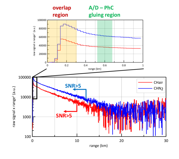
Figure 6: The $L_{\rm E}(s)$ and $L_{\rm R}(s)$ signals in CH_air and CH_N₂, a combination of the A/D and PhC detection are shown for a typical measurement session. The levels corresponding to SNR = 5 are indicated. The areas where the geometrical overlap function has an effect and where the gluing between A/D and PhC is done are shown in the zoom of the range between ground and 1 km height in the bottom panel.

The $L_{\rm E}(s)$ and $L_{\rm R}(s)$ signals, accumulated for about 24 minutes and representing one hour of common observation of RL and AMT are shown in Fig. 6. The ratio between $L_{\rm E}(s)$ and $L_{\rm R}(s)$ is $\sim$ 0.5, comparable to the estimations of the expected signals in CH_air and CH_N₂. The gluing of the A/D and PhC detections has been done in the range around 600 m where the PhC rate is well below 10 MHz for both $L_{\rm E}(s)$ and $L_{\rm R}(s)$. The SNR falls below 5 above 10 km for $L_{\rm E}(s)$ and above 12 km for $L_{\rm R}(s)$. According to our design of the receiver we expect that the geometrical overlap function modulates the Lidar returns from ground up to 300 m.

3.3 Atmospheric Monitoring Telescope

The AMT is a UV air fluorescence cosmic ray telescope that was optimized for this project. The AMT was commissioned in January 2010. Regular measurements started after a 10 month engineering phase on October 8, 2010. In total, 320 hours of data were recorded with the AMT over nine dark periods around new moon. The decommissioning of the RL and the LT in July 2011 entailed the termination of AMT measurements.

3.3.1 Optics

A 3.5 m² spherical mirror of four segments, PMT camera, and UV optical filter comprise the AMT optics. They are the type used in the HiRes-II detector [19]. As a light pulse from the laser travels upward through the atmosphere, a reflected image of the scattered light reaching the mirror sweeps downward across the PMT camera (Fig. 8, bottom left). This light spot crosses the camera in about 30 µs. The spot size is about 2 cm. The field of view of one PMT is 1^∘. A UV filter mounted on the camera increases the contrast of UV light against the night sky background.

There is no direct line of site between the laser and the AMT. The Two Buttes landmark, visible from both sites, was used as a survey reference to establish the AMT azimuth direction. The AMT optical axis, defined as the direction of the sky that is imaged on the center of the camera, was adjusted to 8.72^∘ in elevation and 16.0^∘ in azimuth (CCW from North). After correcting for the difference in altitude and the curvature of the earth, the AMT views the laser between 1.5 km and 10.6 km above ground at the LT (2.7 km and 11.8 km above sea level, respectively).

3.3.2 Infrastructure

The optical components are housed in a custom-built shelter. In Fig. 8, a picture (top left panel) and 3D rendering (bottom right panel) are shown. A roll-up door (top right panel) spans the end of the shelter that forms the optical aperture. Since the shelter points north and away from the sun, this door can be opened safely any hour of the day. A precipitation and ultrasonic wind sensor are read by the slow control system to ensure the door is closed during rainy or windy conditions. The shelter is mounted on four concrete posts with fixtures that permit adjustments to the AMT pointing direction by a few degrees. The AMT is aligned so that the vertical laser track passes near the center of the optical field of view. Adjacent to the AMT shelter is a modified shipping container. This “counting house” holds the data acquisition system and portions of the slow control system. Power and signal cables connect the AMT and the counting house through underground conduits. A local company provides a wireless internet connection to the AMT from a broadcast tower about 4 km away. The AMT door and field of view can be observed remotely by the webcam.

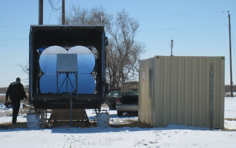
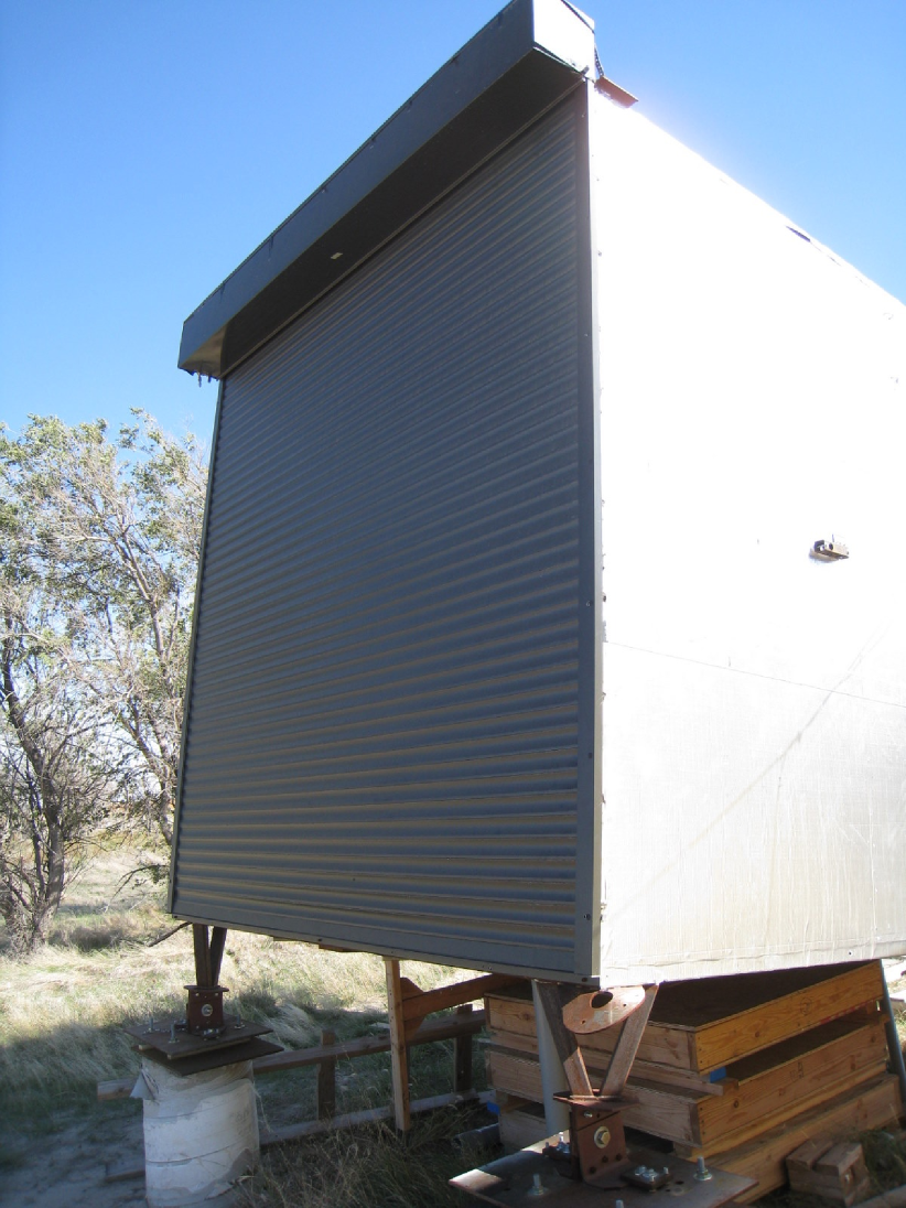
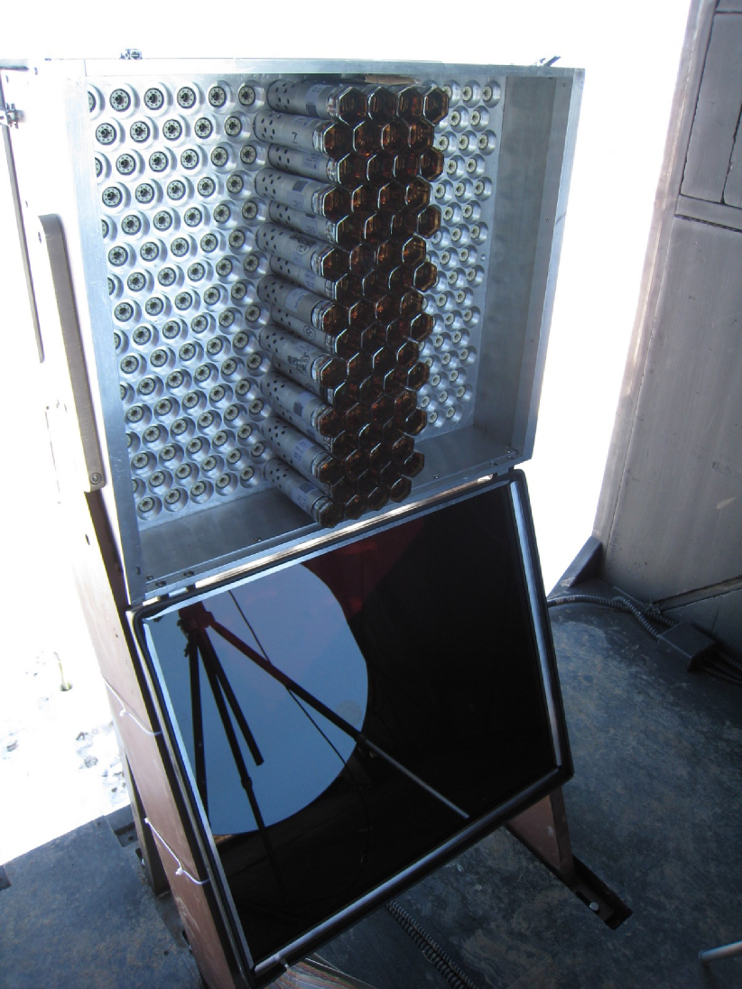
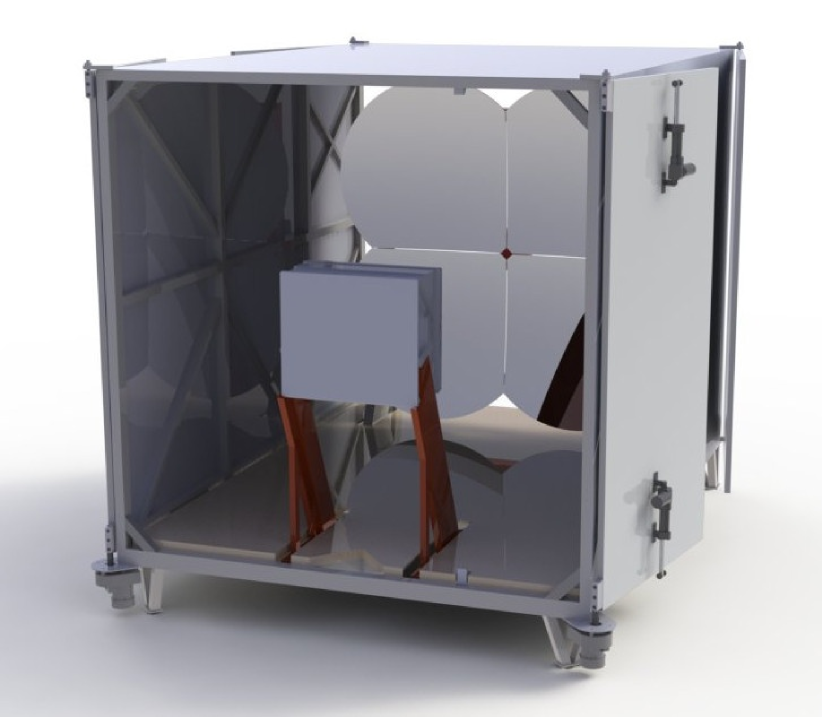
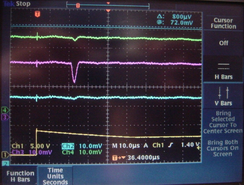
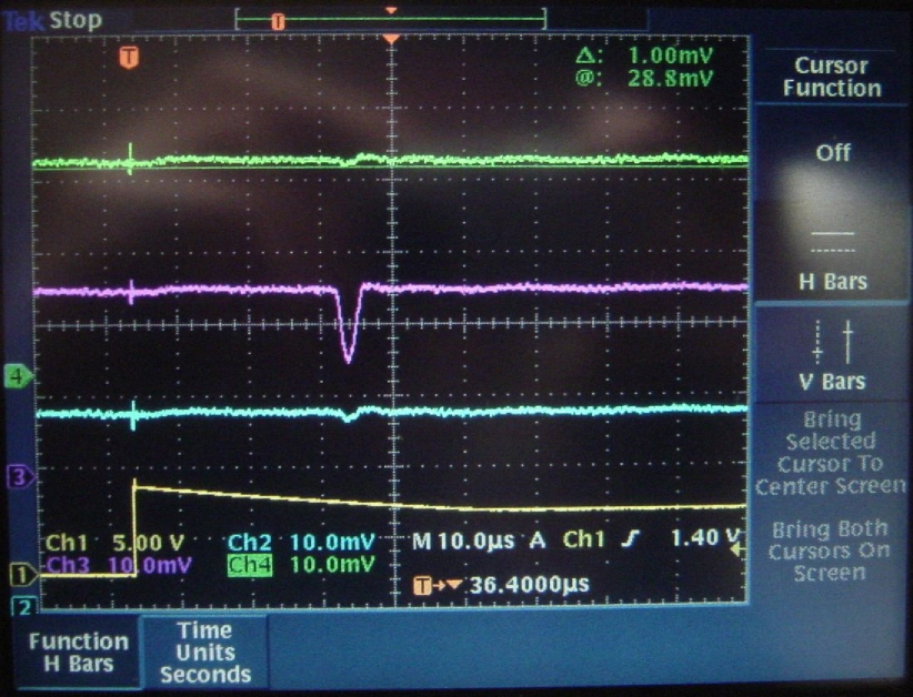
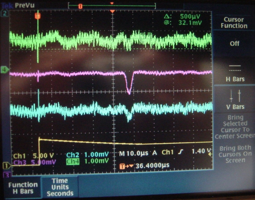
Figure 7: AMT mirror, camera, weather sensors and calibration system are housed in a custom shelter (top left), the adjacent container contains the data acquisition system. A roll-up door can be closed across the entrance aperture (top right). The AMT camera (bottom left) is shown with the UV bandpass optical filter opened. A 3D rendering of the AMT using the CAD design software SolidWorks® (bottom right).

Figure 8: First LT signals seen at the AMT. Left to right correspond to heights of 2.0, 4.9 and 8.5 km a.g.l. Each panel shows 3 signal traces, averaged over 128 laser pulses, by PMTs in the same row. As the path length gets longer, signals shift further in time relative to the external trigger pulse (bottom trace).

3.3.3 Camera and External Trigger

Table 7: Technical specifications and spectral features of the PMTs and bandpass filter.

Photomultiplier model	Photonis XP3802
Photocathode type	Flat hexagonal bialkali
Wavelength sensitivity of photocathode	300–650 nm
Quantum efficiency at 375 nm	30%
Gain (operated)	$\sim 10^{5}$
UV bandpass filter transmission window	300–400 nm
Transmission at 354.7 nm	$\sim$ 80%

The AMT camera is designed to hold 256 PMTs arranged in a 16 $\times$ 16 hexagonal grid. The camera, including the mechanical structure, the PMT/preamp assemblies that are plugged into the camera backplane, and the LV and HV distribution, were developed for the HiRes-II detector [19]. Some specifications on the PMTs can be found in Tab. 7. For this project, the central 3 columns that viewed the LT vertical track were instrumented (Fig. 8, bottom left panel) for a combined field of view of 3.5^∘ in azimuth and 14^∘ in elevation. These 48 PMTs were selected from a larger set that was gain sorted. The photocathode was held at ground with AC coupling (500 µs time constant) applied to the anode signals. The output voltage is the output current multiplied by 3 k$\Omega$. The differential preamp output was read out via equal length twisted pair cables.

A UV bandpass glass filter is mounted in front of the PMTs (some features in Tab. 7). Tests at the Colorado site showed that this filter reduced the night sky background light by about a factor of 2 while transmitting about 80% of the 354.7 nm laser light, which is in agreement with previous measurements [20].

Oscilloscope traces of first light as recorded with individual PMT assemblies in the AMT camera and averaged over 128 shots from the LT, can be seen in Fig. 8. For atmospheric studies 200 laser shots were averaged. The oscilloscope was placed in the counting house and measured the pulses across the twisted pair cables. The first light test also verified the external triggering scheme. A custom GPS module triggered the laser firing time. A second, identical GPS module was placed at the AMT and programmed with a delay to account for the light travel time from the laser to the AMT. This module triggered the oscilloscope during the engineering phase and later the data acquisition system.

Data from a temperature controlled UV LED system at the mirror center and from a vertical nitrogen laser scanned across the field of view were used to flat field the camera. Variable gain preamps in each channel of the front end of the data acquisition electronics were adjusted to do this. The LED system follows the design used in the Pierre Auger Observatory FD drum calibration system [21]. During routine nightly operation, the relative calibration of the PMTs was monitored using the LED system.

3.3.4 Data Acquisition

The camera readout is performed by the pulse shaping and digitization electronics that are also used by the High Elevation Auger Telescope (HEAT) extension [22] at the Pierre Auger Observatory. The AMT readout includes one Second Level Trigger (SLT) board and three First Level Trigger (FLT) boards [2]. The readout is triggered externally. Each trigger prompts the SLT to read out the FLTs and store the event. One FLT board with 22 channels is used per 16 pixel vertical column and records 100 µs of data in 2000 50 ns time bins. The readout software interface program is a modified version of the run control program used for the FD telescopes of the Pierre Auger Observatory.

The DAQ timestamps AMT events so that the recoded traces can be matched to the laser shots fired by the LT. The time is synchronized through the internet once every night using a Network Time Protocol (NTP) server. To keep the time aligned during the run, a one pulse per second signal (1 PPS) is provided by a GPS module.

Figure 9: A schematic of the AMT slow control system.

3.3.5 Slow Control System

Three Single Board Computers (SBCs) control the operation of the AMT. Their main functions and the associated components are shown in Fig. 9. The SBCs and the DAQ are connected via an internal network. The two SBCs inside the AMT shelter are responsible for the slow control systems and the LED calibration system. The LED SBC can fire the LED at different pulse lengths and widths. The system delivers a trigger signal for every LED pulse to trigger the DAQ and records voltage traces for every pulse.

The AMT SBC controls and monitors the door, the low voltage power of the camera, the high voltage of the PMTs and the weather station. The weather station provides a set of temperature, pressure, wind, and precipitation every 5 seconds. A safety daemon program running in the background on the AMT SBC checks if the values for wind and rain are within the safety margins. The SBC shuts the door and powers down the high voltage if wind of more than 7 m s^-1 or rain is measured.

In the counting house, the “Boss” SBC controls the nightly operations. From there, commands can be sent to both the AMT and the LED SBC. A daemon on the Boss reads a set of commands from a text file that specify the nightly operations sequence. The Boss SBC includes the GPS module used to trigger the AMT data acquisition.

The power supply of the Boss, the DAQ and all electronics inside the AMT are secured by UPS, similar to the systems at the LT and RL. In case of main power failure, enough power is available to close the AMT door and shut all systems down securely. All systems are also connected to remote power control units that can switch the power on or off and are controlled via the network by the Boss SBC or manually by an operator.

4 Data Collection and Analysis

The AMT, RL, LT and various subsystems are all operated under computer control. Their nightly operation is sequenced by automation scripts initiated on moonless nights from the Colorado School of Mines campus. Operation and data collection are then monitored remotely by collaborators in Colorado, Germany, and Italy.

4.1 Sequence of Operations

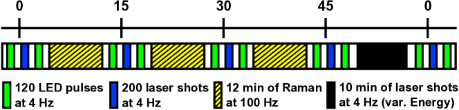
Figure 10: Scheme of the sequence of operations for one hour during combined data taking. 200 laser shots for the AMT are produced every 15 minutes starting at minute 1 of every hour. 120 LED calibration pulses are done before and after every laser set. In the first three quarter hour breaks, the Raman Lidar collects data for about 8 minutes. In the fourth quarter hour space, the laser is fired in AMT mode at different energies.

The RL system and AMT have independent procedures which run in parallel, a scheme of the hourly sequence is shown in Fig. 10. The procedures are synchronized by GPS. Each night, the Raman Lidar system operations start at 2:15 UTC and shut down at 11:00 UTC. Starting at 3:00 UTC, 200 vertical shots for the AMT measurements are fired into the sky on minutes 1, 16, 31 and 46 of each hour. The laser fires at 4 Hz, at 100, 350, 600, and 850 ms after the full second. The data acquisition of the AMT is triggered accordingly by the GPS board of the Boss computer, corrected for the time the light takes to reach the AMT, around 130 µs. In the Raman mode, the laser fires at 100 Hz. Backscattered photons from these laser shots are measured by the Raman system, which collects data for eight minutes during the first three intervals between sets of AMT laser shots. Between minutes 47 and 57, vertical laser shots at lower energies are shot into the sky to check the linearity of the response of the AMT camera.

The moon causes an intolerable level of interference for AMT data collection. Therefore, the hours of AMT operation are dictated by the moon phase. For each night, the hours in which the moonlight background is low are calculated and an AMT command list is produced to perform operations during these hours. During the hours of operation, 120 LED shots are fired before and after each set of AMT laser shots. The LED sends its own trigger to the DAQ each time it fires. The Raman system can operate every night, moonlight does not hinder the operations.

4.2 Monitoring and Nightly Calibration

For the relative calibration of the AMT camera during nightly operations, a UV LED was mounted in the center of the mirror, pointing along the optical axis. Inside this calibration light source, a temperature-controlled UV LED produces short light pulses at 375 nm. The LED was calibrated in the lab relative to calibrated photodiodes by NIST. The LED is of the same type used to calibrate the fluorescence detectors at the Pierre Auger Observatory [23]. Several layers of diffuser material are used to make the light almost isotropic before it reaches the camera. These pulses can be used to keep track of changes in the PMT response. The LED is fired 120 times at a frequency of 4 Hz, one minute before and after the laser shots from the LT, providing two sets of calibration data for each set of laser shots.

The current going through the LED is measured. Comparing the input signal with the output generated by the PMTs as measured by the data acquisition system, a relative calibration constant can be computed to correct the PMT signal. Before calculating this constant, the PMT response has to be corrected for two geometrical effects. The UV LED can be considered as a point source, the camera body with the PMTs is flat, resulting in a smaller signal for PMTs further away from the camera center. The flat camera body also causes a lowered effective area A_eff of the outer PMTs. Accounting for both effects reduces the observed light intensity of the LED to

$$I_{\mathrm{obs}}(\theta)=I_{0}\cdot\frac{A_{\mathrm{eff}}}{4\pi r^{\prime\,2}}=I_{0}\cdot\frac{A_{\mathrm{PMT}}\cdot\cos^{3}\theta}{4\pi r^{2}},$$

where $r$ is the distance between the LED and the center of the camera, $r^{\prime}$ is the distance to a pixel offset from the center vertically by an angle $\theta$.

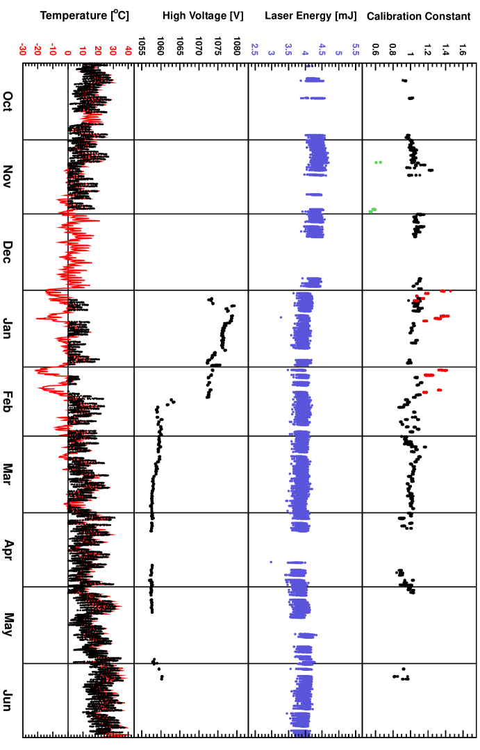
Figure 11: Calibration and monitoring data for the AMT and the LT. In the top panel, the calibration constant for one of the pixels is shown. In the second and third panel, the laser energy and the readout from the high voltage monitor can be seen. On the bottom, the temperature of the weather station at the AMT is shown, together with meteorological model data in red. For more details see text.

The currents of the UV calibration LED are averaged for every calibration set of 120 shots at 4 Hz, lasting 30 seconds in total. In some rare cases, the calibration light source did not fire or the DAQ was not triggered. If neither the calibration before nor the one after a laser run was recorded, the closest in time from a different set of laser shots is used, usually about 15 minutes before or after. The actual calibration constant is calculated for each AMT pixel by dividing the averaged voltage of the LED by the averaged PMT signal for every 120 shot calibration set. This value is then normalized to the calibration constant of an arbitrarily chosen night of data taking to get calibration constants around unity. An absolute calibration of the pixels is not necessary, the algorithm used to extract the aerosol optical depth $\tau_{\mathrm{aer}}$ from the measured laser shots $SL$ relies on the comparison of the measurement to a reference clear night $L_{\rm S}^{\rm clean}$, see Eq. (2.8). Therefore, only the relative calibration of the current and the reference night have to be known, any absolute calibration cancels out.

In Fig. 11, some monitoring data are presented for the entire duration of combined data taking. In the top panel, the calibration constant for one of the AMT pixels in the central column with a field of view closest to the horizon are shown. The average calibration constant is 1.04 with a standard deviation of 0.09. In the second panel, the laser energy as measured with the pick-off probe at the LT. The energy output was stable over the whole operational period. In the third panel the output of a high voltage probe at the AMT camera is displayed. It was installed in January 2010. In February of 2010 a drop in HV is visible. There is no clear explanation for this change, but it is expected that this drop does not impact the measurements.

Also shown in Fig. 11, bottom panel, is the temperature as measured with the weather station at the AMT (black dots). Since the available data have several gaps when the station was not functioning or the temperature was below zero, data from a global meteorological model (GDAS [9]) are used to supplement the data (red line). When comparing the calibration constant with the temperature, it is obvious that unusually high calibration constants correlate with particularly low temperatures. This is most likely due to the calibration LED. Although it is temperature controlled, it seems not to function well below a temperature of $-$8^∘C. For this reason, data recorded under such conditions was discarded, calibration constants for these nights are marked in red in the top panel. In early and late November, wrong gain settings for the preamp of the front end electronics were used accidentally, those calibration constants are plotted in green. Periods of low temperatures and wrong gain settings are discarded as bad periods.

4.3 Collected Data

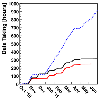
Figure 12: Cumulative number of operational hours of the Raman Lidar (blue dashed) and the AMT (black). Hours where both systems acquired data are drawn in red.

Since each system is capable of performing its startup, data collection and shutdown procedures without an on-site shifter, these systems are monitored remotely. Operations began on October 8, 2010, the systems have been monitored from Golden, Colorado (approximately 500 km from the site), from Karlsruhe, Germany, from L’Aquila, Italy and once from Malargüe, Argentina. The longer period without data taking in November 2010 was due to a failure of the Raman DAQ. The AMT can only operate in nights with low illuminated moon fraction, so about 1.5 weeks before and after new moon. Regular operations were disturbed by broken components like the weather station or the high voltage power supply. Towards the end of measurements in June 2010, the operation of the AMT became more and more difficult, in May 2011 data from two hours and in June 2011 only one hour is available. It was decided to stop operations of the AMT one month earlier, the Raman Lidar was decommissioned in July. In total, 320 hours of data were collected by the AMT, 937 hours by the Raman alone and 251 hours of combined data are available, see Fig. 12. Rejecting bad periods due to bad weather and other causes, 292 AMT and 233 combined hours remain.

The Raman $\tau_{\mathrm{aer}}$ and the backscatter coefficient $\beta_{\mathrm{aer}}$ were estimated using the $L_{\rm E}(s)$ and $L_{\rm R}(s)$ signals in CH_air and CH_N₂, that are a combination of the A/D and PhC detection along a Raman Lidar measurement session. The hourly GDAS molecular atmosphere [9] corresponding to the measurement period is used to estimate the contribution of the Rayleigh scattering processes into the Lidar returns. The GDAS data are available in 3-hourly, global, 1^∘ latitude-longitude (360^∘ by 180^∘) datasets. Each data set consists of surface data and data for 23 constant pressure levels (from sea level up to about 26 km). Among the meteorological fields contained in the GDAS hourly file there are temperature, pressure and relative humidity values from which the molecular number density profile of the atmosphere can be estimated for calculating the Rayleigh backscatter and extinction coefficients as used in equations (2.2)–(2.6). The GDAS grid point closest to the site of the Raman Lidar is 38^∘ north and 102^∘ west, which is East of the town of Lamar.

For this particular analysis, no optical overlap correction was used, both $\tau_{\mathrm{aer}}$ and $\beta_{\mathrm{aer}}$ profiles are valid in a range between about 0.5 km and 5–6 km above ground level. Raman Lidar data were collected during clear and cloudy periods. In total, from 937 hours of data taking, after the quality check, 930 reconstructed hourly profiles of $\tau_{\mathrm{aer}}$ and simultaneous $\beta_{\mathrm{aer}}$ are available, among those profiles about 280 present low clouds.

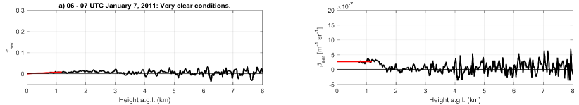
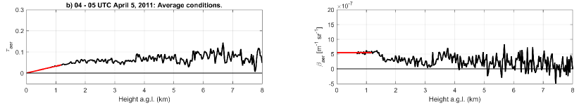
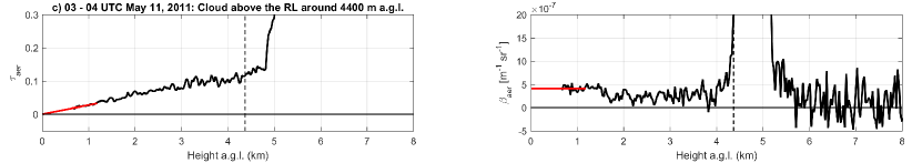
Figure 13: The raw data from the Raman Lidar analysis shown in black, in red the extrapolation to ground. On the left, the vertical aerosol optical depth $\tau_{\mathrm{aer}}$, on the right, the aerosol backscatter coefficient $\beta_{\mathrm{aer}}$. From top to bottom, the Raman data measured during extremely clear (a), average (b) and cloudy conditions (c) are shown.

In Fig. 13, as examples, the raw profiles are drawn in black. The profiles of $\tau_{\mathrm{aer}}$ and $\beta_{\mathrm{aer}}$ are measured during very clear (a) and average (b) conditions, and, in the bottom panel (c), in presence of clouds, as it can be seen in $\beta_{\mathrm{aer}}$. A crude cloud height determination was introduced, if $\beta_{\mathrm{aer}}$ rises above 2 $\times$ 10^-6 m^-1 sr^-1, the minimum cloud height is set, visualized in the panel (c) by a black dashed line.

Every hour during AMT operations, four sets of 200 laser shots are fired by the laser. A set is fired every 15 minutes, resulting in 800 shots per hour. The signal of every pixel is corrected by the calibration constant, then the traces of all pixels are summed and an hourly average is formed.

To analyze the measured data, a reference clear night had to be identified in order to calculate the aerosol optical depth. All available profiles were checked for the highest photon number at the aperture. Two hours in the same night were identified, the chosen reference profiles were measured on January 7, 2011 between the hours of 6 and 8 UTC. This choice was verified by the Raman Lidar data of this night which also shows a quite low aerosol load, see top panel in Fig. 13. Two hours are sufficient for defining a reference night, the number of shots included is 1600.

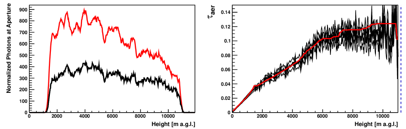
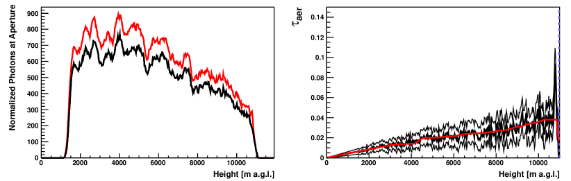
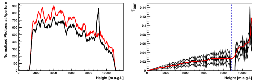
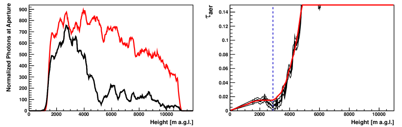
Figure 14: From top to bottom: November 11, 2010, 10–11 UTC: Hazy conditions; December 1, 2010, 4–5 UTC: Clear conditions; December 1, 2010, 5–6 UTC: Laser hit small cloud around 8800 m a.g.l.; December 7, 2010, 4–5 UTC: Cloud obstructing the light above 2800 m a.g.l. Left: Light profiles as measured with the AMT in black, reference clear nights in red. Right: Measured $\tau_{\mathrm{aer}}$ in black with uncertainties, fit $\tau_{\mathrm{aer}}$ in red. The reconstructed minimum cloud height is marked with a blue dashed line.

In Fig. 14, light profiles and aerosol optical depth profiles for four different conditions are shown. In the left panels, the averaged hourly light profile is shown together with the reference clear night. The fine structure of the trace is due to light lost in the gaps between the PMTs of the camera. On the right side, the measured $\tau_{\mathrm{aer}}$ profiles are shown as a thick black line with their uncertainties as thin lines. In red, the fit $\tau_{\mathrm{aer}}$ profiles are superimposed, the minimum cloud height is indicated with a blue dashed line. From top to bottom, hazy (a) and clear conditions (b), as well as two cloud-affected profiles are shown. It should be noted, that the clear profile (b) and the profile where the laser hit a small cloud (c) are only separated by one hour, demonstrating the high variability of the aerosol conditions and the need for hourly aerosol profiles.

The AMT cloud heights agree with the heights determined from the Raman data, only a few profiles are not marked with a cloud by the Raman Lidar where very low clouds are found in the AMT data and vice versa. The Raman Lidar can only detect clouds directly above the laser facility, while the AMT is also affected by clouds in the path between the laser and the detector.

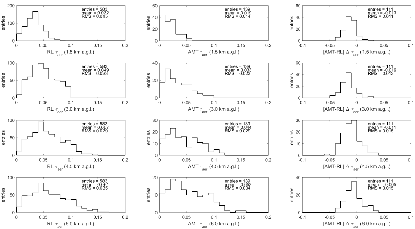
Figure 15: Mean $\tau_{\mathrm{aer}}$ and difference in $\tau_{\mathrm{aer}}$ at 1.5, 3.0, 4.5 and 6.0 km a.g.l. (from upper to lower plot). Left plots: as measured by the Raman Lidar. Middle plots: as measured with the AMT. Right plots: the differences in $\tau_{\mathrm{aer}}$ between the two systems.

The Raman Lidar $\tau_{\mathrm{aer}}$ distributions are shown in the left panels of Fig. 15. A quality cut has been applied to remove the clouds, the $\tau_{\mathrm{aer}}$ has to be less than 0.1, 0.15 and 0.2 at 3, 4.5 and 6 km, respectively. The mean $\tau_{\mathrm{aer}}$ at 1.5 km a.g.l. is 0.032 with an RMS of 0.015, 0.049 with an RMS of 0.023 at 3 km, 0.057 with an RMS of 0.029 at 4.5 km, and at 6 km, the mean is 0.061 with an RMS of 0.035.

The distribution of available AMT $\tau_{\mathrm{aer}}$ profiles after the selection of the cases without clouds, using the same criteria as for the Raman Lidar data, is shown in the middle panels of Fig. 15. The mean $\tau_{\mathrm{aer}}$ at 1.5 km a.g.l. is 0.019 with an RMS 0.014, 0.033 with an RMS of 0.023 at 3 km, 0.044 with an RMS of 0.029 at 4.5 km, and at 6 km, a mean $\tau_{\mathrm{aer}}$ of 0.053 with an RMS of 0.034 is found.

As expected, both the mean $\tau_{\mathrm{aer}}$ and the spread increases with height. In the right panels of Fig. 15, the binned differences in $\tau_{\mathrm{aer}}$ between the two analyses are shown for 1.5, 3, 4.5 and 6 km. Mean differences of $-$0.013 with an RMS of 0.011, $-$0.016 with an RMS of 0.013, $-$0.011 with an RMS of 0.015, and $-$0.005 with an RMS of 0.015 are found, respectively. The differences in $\tau_{\mathrm{aer}}$ between the two systems is discussed in the next section.

5 Results

For the first time, the side-scatter method to obtain vertical aerosol depth profiles can be directly compared with a Raman Lidar. The differences of $\tau_{\mathrm{aer}}$ measurements for periods when both systems recorded data are presented at 1.5, 3, 4.5 and 6 km above ground.

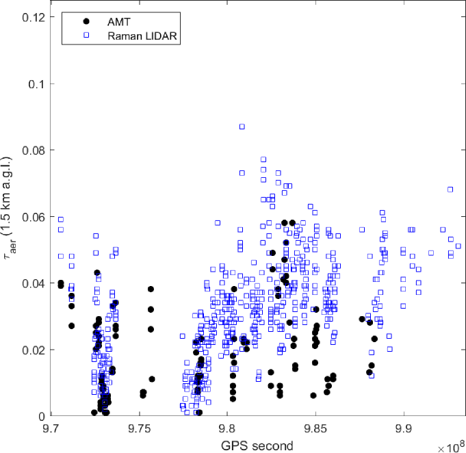
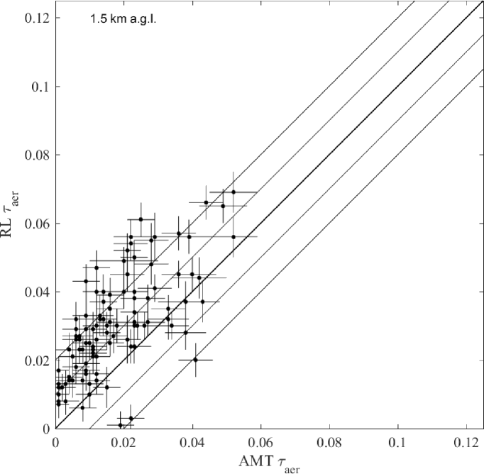
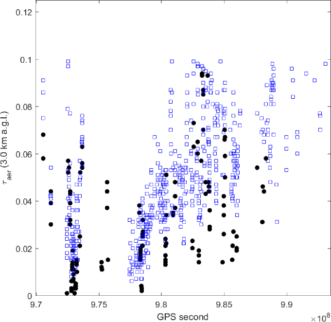
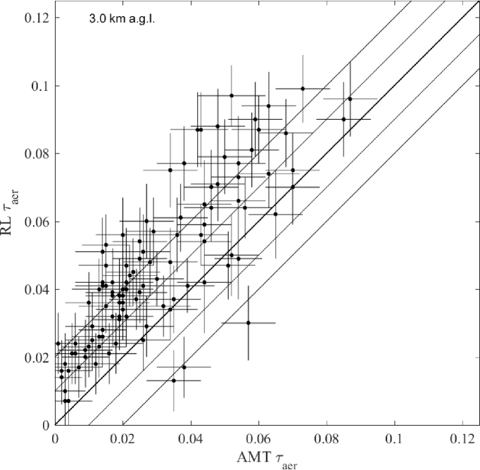
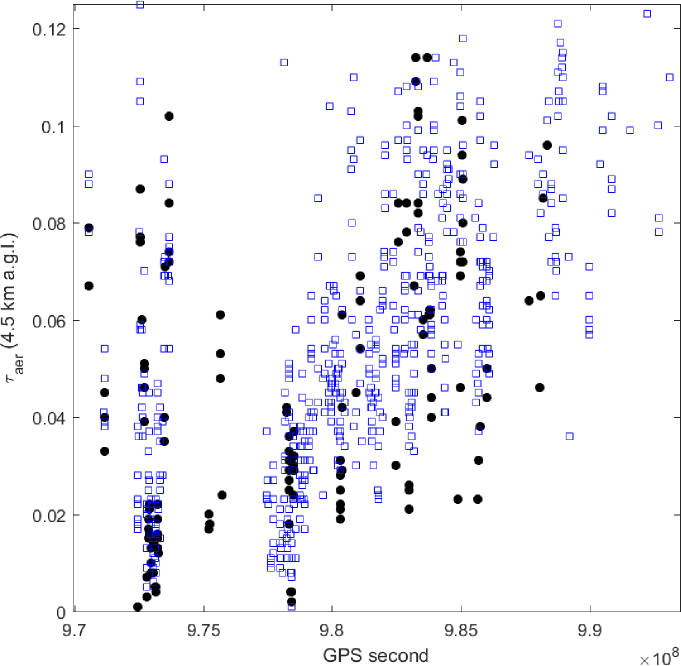
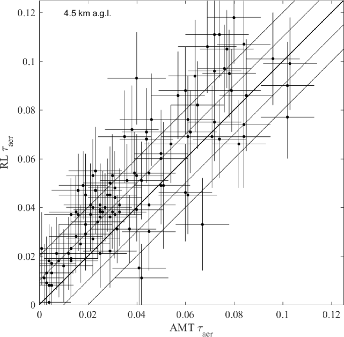
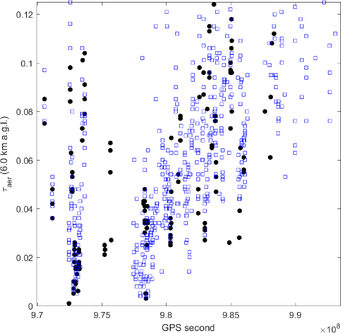
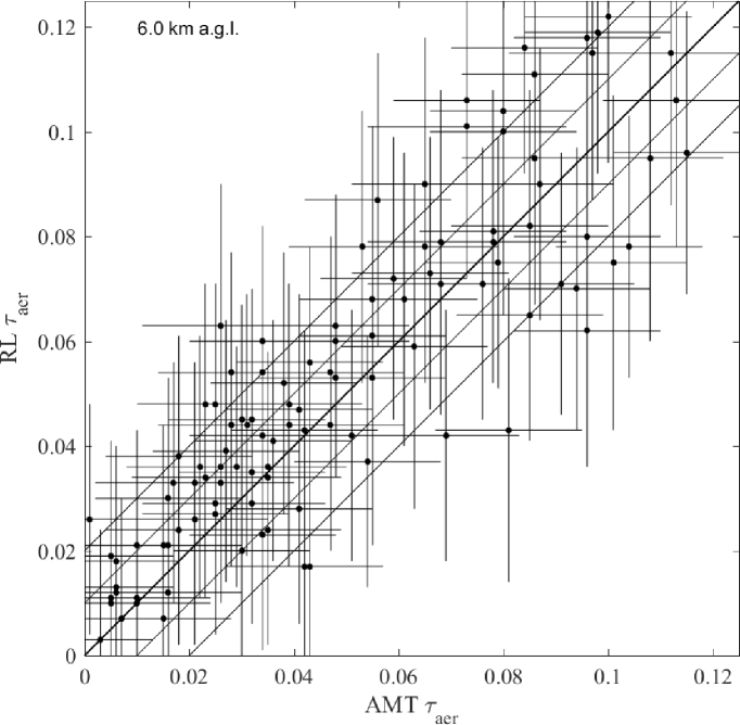
Figure 16: Left: $\tau_{\mathrm{aer}}$ versus time (in GPS seconds) as measured with the AMT (black dots) and the Raman Lidar (blue squares) at 1.5, 3, 4.5 and 6 km a.g.l. between October 1, 2010 and June 30, 2011. Right: $\tau_{\mathrm{aer}}$ measured with the AMT versus Raman Lidar for hours observed with both instruments. The diagonal is indicated with the thick black line, the parallel thin black lines denote a shift in $\tau_{\mathrm{aer}}$ of $\pm$0.01 and $\pm$0.02.

The difference between the $\tau_{\mathrm{aer}}$ measurements of the AMT and of the Raman Lidar at various heights is shown in Fig. 16. In the left column, all data are shown versus time for 1.5, 3, 4.5 and 6 km a.g.l. A clear seasonal trend is visible for both data sets with higher aerosol load in atmosphere during summer. In the right column of Fig. 16, the measurements of $\tau_{\mathrm{aer}}$ at the Raman Lidar are shown versus the AMT data for common measurement periods. At 1.5 km, the Raman Lidar measured $\tau_{\mathrm{aer}}$ is systematically higher than the AMT result, as well as at 3, 4.5 and at 6 km.

There are almost no AMT data in May and in June when the Raman Lidar has measured a largely increasing $\tau_{\mathrm{aer}}$ compared to the previous months, so comparisons in atmospheric conditions with a relatively higher aerosol load are not available.

The Data Normalization method used to retrieve $\tau_{\mathrm{aer}}$ from AMT observations needs a so-called reference night, a measurement in which the atmospheric aerosol content can be considered negligible. The chosen reference clean measurement was on January 7, 2011 between 6 and 8 UTC. The coincident Raman Lidar measurement of $\tau_{\mathrm{aer}}$ shows that the aerosol content is extremely low, but $\tau_{\mathrm{aer}}$ is about 0.01 above 3 km (upper-left panel of Fig. 13), and this value is close to the mean differences between Raman Lidar and AMT data (right panels of Fig. 15).

It is possible that the $\tau_{\mathrm{aer}}$ profiles measured by the two systems can also show a difference in the vertical distribution of the aerosols. The LT and RL are located close to the city of Lamar at a major highway with truck traffic and is surrounded by rangeland, the AMT overlooks planted fields and is far away from both the highway and any kind of civilization. This might cause a difference in the aerosol type and concentration between the AMT and Raman sites. The AMT measurements are dominated by the transmission, not the scattering out of the laser. The difference in surroundings could explain part of the differences and could also be a source of seasonal variations.

6 Conclusion

The Raman Lidar and AMT detector described in this paper were set up in the field near Lamar, Colorado, USA. Both systems were operated remotely for a period of 11 months. A comparison between between the elastic side-scatter and Raman back-scatter methods of aerosol optical depth was obtained. To our knowledge this is the first time that such a comparison has been made systematically. A correlation between the measurements was observed. A systematic offset was also observed. The Raman system obtained higher values of aerosol optical depth than did the elastic side-scatter system. The most likely reason for this offset is that the nominally clear “reference” nights that were used to normalize the elastic side-scatter data were not aerosol free. Systematic horizontal non-uniformity of the atmosphere clarity between the two instruments may also have contributed to the observed bias. The Raman system was located in a ranching area relatively close to the small city of Lamar, the side-scatter detector was located in a farmed area with many fields.

The Raman Lidar system described in this paper has now been relocated to the central laser facility (CLF) of the Pierre Auger Cosmic Ray Observatory in Mendoza province, Argentina. A more detailed atmospheric measurement program is in progress. This program uses the Raman backscatter receiver located at the CLF and optical fluorescence telescopes located at four sites on the perimeter of the 3000 km² observatory.

References

- [1] OpenStreetMap contributors, OpenStreetMap, 2014.
- [2] The Pierre Auger Collaboration, J. Abraham et al., The Fluorescence Detector of the Pierre Auger Observatory, Nucl. Instr. Meth. A620 (2010) 227–251, [arXiv:0907.4282].
- [3] The High Resolution Fly’s Eye (HiRes) Collaboration, R. U. Abbasi et al., Techniques for measuring atmospheric aerosols at the High Resolution Fly’s Eye experiment, Astropart. Phys. 25 (2006) 74–83, [astro-ph/0512423].
- [4] The Pierre Auger Collaboration, P. Abreu et al., Techniques for measuring aerosol attenuation using the Central Laser Facility at the Pierre Auger Observatory, JINST 8 (2013) 04009, [arXiv:1303.5576].
- [5] The Pierre Auger Collaboration, J. Abraham et al., A Study of the Effect of Molecular and Aerosol Conditions in the Atmosphere on Air Fluorescence Measurements at the Pierre Auger Observatory, Astropart. Phys. 33 (2010) 108–129, [arXiv:1002.0366].
- [6] B. Fick et al., The Central Laser Facility at the Pierre Auger Observatory, JINST 1 (2006) 11003.
- [7] G. Pappalardo et al., Aerosol LIDAR Intercomparison in the Framework of the EARLINET Project 3: Raman LIDAR Algorithm for Aerosol Extinction, Backscatter, and LIDAR Ratio, Appl. Optics 43 (2004) 537–538.
- [8] D. Müller, A. Ansmann, I. Mattis, M. Tesche, U. Wandinger, D. Althausen, and G. Pisani, Aerosol-type-dependent lidar ratios observed with Raman lidar, J. Geophys. Res. 112 (2007) D16202.
- [9] NOAA Air Resources Laboratory (ARL), Global Data Assimilation System (GDAS1) Archive Information, Tech. rep., 2004.
- [10] C. Bockmann et al., Aerosol LIDAR Intercomparison in the Framework of the EARLINET Project 2: Aerosol Backscatter Algorithms, Appl. Optics 43 (2004) 977–989.
- [11] A. A. Kokhanovsky, Variability of the phase function of atmospheric aerosols at large scattering angles, J. of Atm. Sci. 55 (1998) 314–320.
- [12] H. A. MacLeod, Thin-Film Optical Filters. Taylor & Francis, 4 ed., 2010.
- [13] U. Wandinger, Raman LIDAR, vol. 102, pp. 241–271. Springer, 233 Spring St., New York, NY 10013, United States, LIDAR: Range Resolved Optical Remote Sensing of the Atmosphere, Springer Series in Optical Sciences ed., 2004.
- [14] S. Chiao-Yao, Spectral structure of laser light scattering revised: bandwindths of nonresonant scattering LIDARs, Appl. Optics 40 (2001) 4875–4884.
- [15] D. N. Whiteman, Examination of the traditional Raman LIDAR technique. I Evaluating the temperature-dependent LIDAR equations, Appl. Optics 42 (2003) 2571–2592.
- [16] B. J. Kross, S. Majewski, C. J. Zorn, and L. A. Majewski, Flexible liquid core light guide with focusing and light shaping attachments, 1997. US Patent #5684908.
- [17] G. Nath, Lightguide filled with a liquid containing dimethylsulfoxide, 1999. US Patent #5857052.
- [18] G. Nath, Flexible lightguide with a liquid core, 2001. US Patent #6314226.
- [19] J. Boyer, B. Knapp, E. Mannel, and M. Seman, FADC based DAQ for HiRes Fly’s Eye, Nucl. Instr. Meth. A482 (2002) 457–474.
- [20] The High Resolution Fly’s Eye (HiRes) Collaboration, L. Wiencke et al., Radio-controlled Xenon Flashers for Atmospheric Monitoring at the HiRes Cosmic Ray Observatory, Nucl. Instr. Meth. A428 (1999) 593–607.
- [21] J. T. Brack, R. Cope, A. Dorofeev, B. Gookin, J. L. Harton, Y. Petrov, and A. C. Rovero, Absolute calibration of a large-diameter light source, JINST 8 (2013), no. 05 P05014, [arXiv:1305.1329].
- [22] The Pierre Auger Collaboration, H. J. Mathes et al., The HEAT telescopes of the Pierre Auger Observatory: status and first data, in Proc. 32nd ICRC, vol. 3, (Beijing, China), pp. 149–152, 2011. arXiv:1107.4807.
- [23] The Pierre Auger Collaboration, J. Abraham et al., The Fluorescence Detector of the Pierre Auger Observatory, Nucl. Instr. Meth. A620 (2010) 227–251, [arXiv:0907.4282].