$L_{\mu}-L_{\tau}$ gauge-boson production from lepton flavor violating $\tau$ decays at Belle II

Abstract

$L_{\mu}-L_{\tau}$ gauge boson ($Z^{\prime}$) with a mass in the MeV to GeV region can resolve not only the muon $g-2$ excess, but also the gap in the high-energy cosmic neutrino spectrum at IceCube. It was recently proposed that such a light gauge boson can be detected during the Belle II experiment with a luminosity of 50 ab^-1 by the $e^{+}e^{-}\to\gamma+\not{E}$ process through the kinetic mixing with the photon, where the missing energy $\not{E}$ is from the $Z^{\prime}\to\bar{\nu}\nu$ decays. We study the phenomenological implications when a pair of singlet vector-like leptons carrying different $L_{\mu}-L_{\tau}$ charges are included, and a complex singlet scalar ($\phi_{S}$) is introduced to accomplish the spontaneous $U(1)_{L_{\mu}-L_{\tau}}$ symmetry breaking. It is found that the extension leads to several phenomena of interest, including (i) branching ratio (BR) for $h\to\mu\tau$ can be of the order of $10^{-3}$; (ii) $\phi_{S}$-mediated muon $g-2$ can be of the order of $10\times 10^{-10}$; (iii) BR for $\tau\to\mu\phi^{*}_{S}\to\mu Z^{\prime}Z^{\prime}$ can be $10^{-8}$, and (iv) kinetic mixing between the $Z^{\prime}$ boson and photon is sensitive to the relative heavy lepton masses. The predicted BRs for $\tau\to(3\mu+\not{E},5\mu$) through the leptonic $Z^{\prime}$ decays can reach a level of $10^{-9}$, in which the results fall within the sensitivity of the Belle II in the search for the rare tau decays.

I Introduction

A $Z^{\prime}$ gauge boson, dictated by an anomaly-free $U(1)_{L_{\mu}-L_{\tau}}$ gauge symmetry He:1990pn ; Foot:1994vd , has been broadly studied. Especially, the $Z^{\prime}$ boson with a mass in the range between MeV and GeV can help explain observed anomalies, such as the muon anomalous magnetic moment (muon $g-2$) Altmannshofer:2016brv ; Gninenko:2014pea ; Gninenko:2001hx , and deficiencies in the high-energy cosmic neutrino spectrum reported by IceCube Aartsen:2014gkd ; Araki:2014ona ; Kamada:2015era ; DiFranzo:2015qea ; Araki:2015mya . In addition, the $U(1)_{\mu-\tau}\equiv U(1)_{L_{\mu}-L_{\tau}}$ gauge model can be also used to resolve the largely unexpected lepton-flavor nonuniversality in semileptonic $B$ decays Altmannshofer:2014cfa ; Crivellin:2015mga ; Altmannshofer:2016jzy , Higgs $h$ lepton flavor violating (FLV) decays Crivellin:2015mga ; Heeck:2014qea ; Altmannshofer:2016oaq ; Heeck:2016xkh , and dark matter and/or neutrino mass Baek:2015fea ; Biswas:2016yan ; Patra:2016shz ; Baek:2015mna ; Lee:2017ekw .

Recently, there has been some progress made with detecting the light $Z^{\prime}$ boson in experiments and limiting the ranges of $Z^{\prime}$ mass $m_{Z^{\prime}}$ and gauge coupling $g_{Z^{\prime}}$, which are used to fit the muon $g-2$ anomaly. For instance, according to neutrino trident production processes, which were measured by the CHARM-II collaboration Geiregat:1990gz and CCFR collaboration Mishra:1991bv , it was shown that $m_{Z^{\prime}}\gtrsim 400$ MeV and $g_{Z^{\prime}}>{\rm few}\times 10^{-3}$ are excluded Altmannshofer:2014pba . Based on a observation of cross-section of the $e^{+}e^{-}\to\mu^{+}\mu^{-}Z^{\prime}$, $Z^{\prime}\to\mu^{+}\mu^{-}$ channel, which was recently measured by the BABAR collaboration at a 90% confidence level (CL) TheBABAR:2016rlg , the bound of $g_{Z^{\prime}}<0.7\times 10^{-3}$ at $m_{Z^{\prime}}\approx 0.22$ GeV can be obtained. The ranges of $m_{Z^{\prime}}\subset(1,10)$ MeV and $g_{Z^{\prime}}\subset(0.1,1)\times 10^{-3}$ were badly narrowed Harnik:2012ni by the measurement of ${}^{7}Be$ solar neutrino scattering off the electron in the Borexino experiment Bellini:2011rx , where the $\nu$-$e$ scattering occurred through loop-induced kinetic mixing between the electromagnetic and $Z^{\prime}$ gauge fields. Although the $m_{Z^{\prime}}$ and $g_{Z^{\prime}}$ parameter spaces for explaining the muon $g-2$ excess are not completely excluded, the allowed ranges are strictly bounded by the experiments above.

A detection of the light $Z^{\prime}$ gauge boson via the process $e^{+}e^{-}\to\gamma+\not{E}$ at the Belle II, which will record an unprecedented data sample of 50 ab^-1, was recently proposed in Araki:2017wyg ; Kaneta:2016uyt , where $\not{E}$ is the missing energy from the $Z^{\prime}\to\bar{\nu}\nu$ decays, and the $Z^{\prime}$ boson is produced through kinetic mixing with the photon. Although kinetic mixing was also involved in the Borexino $\nu$-$e$ scattering experiment, it was found that the loop-induced mixing in the $e^{+}e^{-}\to\gamma Z^{\prime}$ process is dependent on the $q^{2}=m^{2}_{Z^{\prime}}$, whereas the mixing in the solar neutrino experiment is a constant in $q^{2}$ due to the low energy neutrinos. The kinetic mixing parameters in the both processes are respectively written as Araki:2017wyg :

$$\epsilon_{\rm Belle} =\frac{eg_{Z^{\prime}}}{2\pi^{2}}\int^{1}_{0}dx\,x(1-x)\ln\frac{m^{2}_{\tau}-x(1-x)q^{2}}{m^{2}_{\mu}-x(1-x)q^{2}}\,,\quad\epsilon_{\nu e}=\frac{eg_{Z^{\prime}}}{6\pi^{2}}\ln\frac{m_{\tau}}{m_{\mu}}\,.$$ (1)

It has been concluded that with a Belle-II integrated luminosity of 50 ab^-1, the significance of an $e^{+}e^{-}\to\gamma+\not{E}$ process higher than $3\sigma$ significance can be reached, where the sensitive regions are $m_{Z^{\prime}}\lesssim 1$ GeV and $g_{Z^{\prime}}\gtrsim 0.8\times 10^{-3}$.

If we examine the light $Z^{\prime}$ gauge boson together with the spontaneous $U(1)_{\mu-\tau}$ symmetry breaking method, it can be found that in addition to the $m_{Z^{\prime}}$ and $g_{Z^{\prime}}$ parameters, the $U(1)_{\mu-\tau}$ gauge model needs at least one more new free parameter to dictate the mass of a scalar boson, in which the scalar field only carries the $U(1)_{\mu-\tau}$ charge and is responsible for the symmetry breaking. If we employ a complex singlet scalar field ($\phi_{S}$) to accomplish the symmetry breaking, the $\phi_{S}$-$Z^{\prime}$-$Z^{\prime}$ coupling from the kinetic term can lead to the $\phi_{S}\to Z^{\prime}Z^{\prime}$ decay when $m_{S}>2m_{Z^{\prime}}$ is satisfied. If the singlet scalar can be produced with a sizable cross section, the light $Z^{\prime}$ can then be generated through the $\phi_{S}$ decay. However, if the $\phi_{S}$ field only couples to the leptons via the Yukawa interactions, we cannot have the $SU(2)_{L}\times U(1)_{Y}\times U(1)_{\mu-\tau}$ gauge invariant Yukawa couplings because the left-handed and right-handed leptons are $SU(2)_{L}$ doublets and singlets, respectively. Thus, it is difficult to generate the singlet scalar boson and detect the $Z^{\prime}$ signal through the $\phi_{S}\to Z^{\prime}Z^{\prime}$ channel.

We find that if two singlet vector-like leptons, which carry different $U(1)_{\mu-\tau}$ charges, are added to the model, probing the light $Z^{\prime}$ through $\phi_{S}\to Z^{\prime}Z^{\prime}$ can then be achieved. The resulting model not only is $U(1)_{Y}$ and $U(1)_{\mu-\tau}$ gauge anomaly-free, but it also removes the scale dependence of loop-induced kinetic mixing. As a consequence, several phenomena of interest are induced, including (i) LFV branching ratios (BRs) for the $h,\phi_{S}\to\mu\tau$ decays can be of the order of $10^{-3}$; (ii) muon $g-2$ from the same LFV effects can achieve a level of $10^{-9}$; (iii) BR for $\tau\to\mu\phi^{*}_{S}\to\mu Z^{\prime}Z^{\prime}$ can be of the order of $10^{-8}$; (iv) the kinetic mixing of Eq. (1) is modified and becomes sensitive to the relatively heavy lepton masses.

With 50 ab^-1 of data accumulated at the Belle II, the sample of $\tau$ pairs can be increased up to around $5\times 10^{10}$, where the sensitivity necessary to observe the LFV $\tau$ decays can reach $10^{-10}-10^{-9}$, depending on the processes Aushev:2010bq . If $m_{Z^{\prime}}>2m_{\mu}$ and $BR(Z^{\prime}\to\mu^{+}\mu^{-})\times BR(Z^{\prime}\to\bar{\nu}\nu,\mu^{+}\mu^{+})\sim 0.2$, we will show that the BRs for the $\tau\to 3\mu+\not{E}$ and $\tau\to 5\mu$ decays can be ${\cal O}(10^{-9})$ in the extension of the SM. Intriguingly, the resulting BRs of the new tau decay channels are located in the Belle II sensitivity. Since $\tau\to 3\mu$ and $\tau\to(e,\mu)\gamma$ are suppressed in this model, the detectable $\tau\to 3\mu+\not{E}$ and $\tau\to 5\mu$ decays can be used as the characteristics that distinguish them from other models, which have sizable BRs for the $\tau\to 3\mu$ and $\tau\to(e,\mu)\gamma$ decays.

The E821 experiment at the Brookhaven National Laboratory (BNL) Bennett:2006fi revealed the uncertainty of the measured muon $g-2$ to be 0.54 ppm, and a result of over a $3\sigma$ deviation from the SM prediction was obtained. The new muon $g-2$ measurements performed in the E989 experiment at Fermilab and the E34 experiment at J-PARC will aim for a precision of 0.14 ppm Grange:2015fou and 0.10 ppm Otani:2015jra , respectively. Thus, the muon $g-2$ induced by the LFV effects in this model can be strictly bounded with more accurate measurements. Hence, in this work, we plan to show the impacts on lepton-flavor conservation and the LFV phenomena when $U(1)_{\mu-\tau}$ gauge symmetry and two singlet vector-like leptons are introduced to the SM.

The paper is organized as follows. In Sec. II, we introduce the $U(1)_{\mu-\tau}$ extension of the SM by adding two singlet vector-like leptons. The new Yukawa, $Z$, and $Z^{\prime}$ couplings are derived in this section. We show the numerical analysis on the phenomena of interest in Sec. III, where they include $h\to\mu\tau$, muon $g-2$, rare $\tau$ decays, and the influence on the $e^{+}e^{-}\to\gamma Z^{\prime}$. The summary is given in Sec. IV.

II Gauged $L_{\mu}-L_{\tau}$ Model

In the following, we begin to introduce the new interactions in the extension of the SM. In a gauged $L_{\mu}-L_{\tau}$ model, we add two singlet vector-like leptons ($\ell_{4,5}$) and a complex singlet scalar field ($S$) into the SM, where the $S$ field is responsible for the spontaneous $U(1)_{\mu-\tau}$ symmetry breaking, and the heavy leptons lead to lepton-flavor changing neutral currents (LFCNCs) through the Yukawa couplings. In order to obtain the Higgs lepton-flavor violation and remove the scale dependence of the loop-induced kinetic mixing between the photon and the $Z^{\prime}$ gauge boson, the $U(1)_{\mu-\tau}$ charges of $\ell_{4}$ and $\ell_{5}$ must be opposite in sign. When the charge of $\ell_{4}$ is determined, the charge of $S$ then is certain. For clarity, we show the $U(1)_{\mu-\tau}$ charges of the leptons and $S$ field in Table 1. Accordingly, the Yukawa interactions, which satisfy the $SU(2)_{L}\times U(1)_{Y}\times U(1)_{\mu-\tau}$ gauge symmetry, are written as:

$$-{\cal L}_{Y} =Y_{\ell}\bar{L}_{\ell}H\ell_{R}+y_{\mu}\bar{L}_{\mu}H\ell_{4R}+y_{\tau}\bar{\ell}_{4L}\tau_{R}S+m_{4L}\bar{\ell}_{4L}\ell_{4R}+y^{\prime}_{\tau}\bar{L}_{\tau}H\ell_{5R}$$

$$+y^{\prime}_{\mu}\bar{\ell}_{5L}\mu_{R}S^{\dagger}+y_{S}\bar{\ell}_{4L}\ell_{5R}S+y^{\prime}_{S}\bar{\ell}_{5L}\ell_{4R}S^{\dagger}+m_{5L}\bar{\ell}_{5L}\ell_{5R}+H.c.\,,$$ (2)

where $L_{\ell}$ denotes the SM doublet lepton, $f_{R(L)}=P_{R(L)}f$ with $P_{R(L)}=(1\pm\gamma_{5})/2$; $H$ is the SM Higgs doublet, and $m_{4L,5L}$ are the heavy lepton masses. The electroweak and $U(1)_{\mu-\tau}$ symmetries can be spontaneously broken through $\langle H\rangle=(v+h)/\sqrt{2}$ and $\langle S\rangle=(v_{S}+\phi_{S})/\sqrt{2}$, where $v(v_{S})$ is the vacuum expectation value (VEV) of the $H(S)$ field. From Eq. (2), it can be seen that $\ell_{4}$ and $\ell_{5}$ can mix together through the $y_{S}\bar{\ell}_{4}\ell_{5}S$ term when the $U(1)_{\mu-\tau}$ symmetry is broken. In order to simplify the following formulation, we assume $y^{\prime}_{S}=y_{S}$ and take the basis, $\ell^{\prime}_{4}=\cos\alpha\ell_{4}-\sin\alpha\ell_{5}$ and $\ell^{\prime}_{5}=\sin\alpha\ell_{4}+\cos\alpha\ell_{5}$, so that the $2\times 2$ mass matrix of $\ell_{4}$ and $\ell_{5}$ is diagonalized as:

$$\left(\begin{array}[]{cc}m_{L1}&0\\ 0&m_{L2}\end{array}\right)=\left(\begin{array}[]{cc}\cos\alpha&-\sin\alpha\\ \sin\alpha&\cos\alpha\end{array}\right)\left(\begin{array}[]{cc}m_{4L}&\frac{y_{S}v_{S}}{\sqrt{2}}\\ \frac{y_{S}v_{S}}{\sqrt{2}}&m_{5L}\end{array}\right)\left(\begin{array}[]{cc}\cos\alpha&\sin\alpha\\ -\sin\alpha&\cos\alpha\end{array}\right)\,,$$ (3)

where the $m_{L1}$, $m_{L2}$, and the mixing angle $\alpha$ can be related to the $m_{4L,5L}$ and $y_{S}v_{S}$ parameters as:

$$m_{L1,L2} =\frac{1}{2}\left(m_{4L}+m_{5L}\pm\sqrt{(m_{5L}-m_{4L})^{2}+2y^{2}_{S}v^{2}_{S}}\right)\,,$$

$$\tan 2\alpha =\frac{\sqrt{2}y_{S}v_{S}}{m_{5L}-m_{4L}}\,.$$ (4)

We note that in general, the SM Higgs can mix with the scalar $\phi_{S}$ via the scalar potential. Since the mixing is a new free parameter, in order to avoid the constraint resulting from the precision Higgs measurements, hereafter, we consider the mixing to be small and neglect its contributions.

Table 1: $U(1)_{\mu-\tau}$ charges of leptons and $S$ field.

	$e$	$\mu$	$\tau$	$\ell_{4}$	$\ell_{5}$	$S$
$U(1)$	0	1	$-1$	1	$-1$	$2$

Since the model involves a new scalar field $S$, to understand its properties, we write the gauge invariant scalar potential as:

$$V= -\mu_{H}^{2}H^{\dagger}H-\mu_{S}^{2}S^{\dagger}S+\lambda_{H}(H^{\dagger}H)^{2}+\lambda_{S}(S^{\dagger}S)^{2}+\lambda_{HS}(H^{\dagger}H)(S^{\dagger}S)\,$$ (5)

where $\mu^{2}_{H,S}$ and $\lambda_{H,S}$ are positive parameters. Based on the minimum condition, the VEVs of the scalar fields $H$ and $S$ can be obtained as:

$$\frac{\partial V}{\partial v} =v\left(-\mu_{H}^{2}+\lambda_{H}v^{2}+\frac{1}{2}\lambda_{HS}v_{S}^{2}\right)=0,$$

$$\frac{\partial V}{\partial v_{S}} =v_{S}\left(-\mu_{S}^{2}+\lambda_{S}v_{S}^{2}+\frac{1}{2}\lambda_{HS}v^{2}\right)=0.$$ (6)

With the assumption of $\lambda_{HS}\ll 1$, we obtain $v\simeq\sqrt{\mu_{H}^{2}/\lambda_{H}}$ and $v_{S}\simeq\sqrt{\mu_{S}^{2}/\lambda_{S}}$. From the scalar potential, the mass-squared matrix for the $h$ and $\phi_{S}$ is expressed as:

$$M_{\phi}^{2}=\begin{pmatrix}2\mu_{H}^{2}&\lambda_{HS}vv_{S}\\ \lambda_{HS}vv_{S}&2\mu_{S}^{2}\end{pmatrix}.$$ (7)

The eigenvalues and eigenstates of Eq. (7) are then obtained as:

$$m^{2}_{H_{1},H_{2}}=(\mu_{H}^{2}+\mu_{S}^{2})\pm\sqrt{(\mu_{H}^{2}-\mu_{S}^{2})^{2}+\lambda_{HS}vv_{S}},$$

$$\begin{pmatrix}H_{1}\\ H_{2}\end{pmatrix}=\begin{pmatrix}\cos\phi&\sin\phi\\ -\sin\phi&\cos\phi\end{pmatrix}\begin{pmatrix}\phi_{S}\\ h\end{pmatrix},\quad\tan 2\phi=\frac{\lambda_{HS}vv_{S}}{\mu_{H}^{2}-\mu_{S}^{2}},$$ (8)

where $H_{2}$ is the SM-like Higgs boson; and the mass hierarchy $m_{H_{1}}<m_{H_{2}}$ is assumed in this paper. The mixing angle $\phi$ can be constrained by the SM Higgs precision measurements. Especially, when $m_{H_{2}}>2m_{H_{1}},2m_{Z^{\prime}}$, the $H_{2}\to H_{1}H_{1}$ and $H_{2}\to Z^{\prime}Z^{\prime}$ decays will be opened. Since the mixing angle $\phi$ is irrelevant to our study, in the following analysis, we take $\phi\ll 1$, $H_{2}\simeq h$, and $H_{1}\simeq\phi_{S}$. As a result, we have $v_{S}\simeq m_{S}/\sqrt{2\lambda_{S}}$; that is, $v_{S}\sim 100$ GeV and $m_{S}\sim 10$ GeV can be achieved when $\lambda_{S}\sim 5\times 10^{-3}$.

In order to obtain the $Z^{\prime}$ mass and the $S$ gauge coupling to the $Z^{\prime}$ boson, we write the covariant derivative of the $S$ field to be $D_{\mu}=\partial_{\mu}+ig_{Z^{\prime}}X_{S}Z^{\prime}_{\mu}$, where $X_{S}=2$ is the $U(1)_{\mu-\tau}$ charge of the $S$ field. With $\langle S\rangle=(v_{S}+\phi_{S})/\sqrt{2}$, the $Z^{\prime}$ mass and $\phi_{S}-Z^{\prime}-Z^{\prime}$ coupling can be obtained through the kinetic term as:

$$(D^{\mu}S)^{\dagger}(D_{\mu}S) \supset\frac{1}{2}(v_{S}+\phi_{S})^{2}g^{2}_{Z^{\prime}}X^{2}_{S}Z^{\prime}_{\mu}Z^{\prime\mu}\,,$$

$$m_{Z^{\prime}} =2g_{Z^{\prime}}v_{S}\,,\quad\phi_{S}-Z^{\prime}-Z^{\prime}:\frac{2m^{2}_{Z^{\prime}}}{v_{S}}g_{\mu\nu}\,.$$ (9)

After electroweak and $U(1)_{\mu-\tau}$ symmetry breaking, the lepton-flavor mixing information can be obtained from Eq. (2). If we combine the SM leptons and the heavy leptons to form a multiplet state in flavor space, denoted by $\ell^{\prime T}=(\boldsymbol{\ell\,,\Psi}_{\ell})$ with $\boldsymbol{\ell}=(e,\mu,\tau)$ and $\boldsymbol{\Psi}^{T}_{\ell^{\prime}}=(\ell^{\prime}_{4},\ell^{\prime}_{5})$, the $5\times 5$ lepton mass matrix can be written as:

$$\bar{\ell}^{\prime}_{L}M_{\ell^{\prime}}\ell^{\prime}_{R}=\left(\begin{array}[]{cc}\boldsymbol{\bar{\ell}}_{L}\,,&\boldsymbol{\bar{\Psi}}_{\ell L}\end{array}\right)\left(\begin{array}[]{c|c}~{}~{}~{}{\boldsymbol{m}_{\ell}}_{3\times 3}{}{}{}&\boldsymbol{\delta m}_{1}\\ \hline\cr\boldsymbol{\delta m}^{T}_{2}&\boldsymbol{m}_{L}\end{array}\right)_{5\times 5}\left(\begin{array}[]{c}\boldsymbol{\ell}_{R}\\ \boldsymbol{\Psi}_{\ell R}\end{array}\right)\,,$$ (10)

where diag$\boldsymbol{m_{\ell}}=(m_{e},m_{\mu},m_{\tau})$, $m_{f}=vY_{f}/\sqrt{2}$, diag$\boldsymbol{m}_{L}=(m_{L1},m_{L2})$, and $\boldsymbol{\delta m}_{1,2}$ are given by:

$$\boldsymbol{\delta m}^{T}_{1} =\left(\begin{array}[]{ccc}0\,,&\frac{vy_{\mu}}{\sqrt{2}}c_{\alpha}\,,&-\frac{vy^{\prime}_{\tau}}{\sqrt{2}}s_{\alpha}\\ 0\,,&\frac{vy_{\mu}}{\sqrt{2}}s_{\alpha}\,,&\frac{vy^{\prime}_{\tau}}{\sqrt{2}}c_{\alpha}\end{array}\right)\,,~{}~{}\boldsymbol{\delta m}^{T}_{2}=\left(\begin{array}[]{ccc}0\,,&-\frac{v_{S}y^{\prime}_{\mu}}{\sqrt{2}}s_{\alpha}\,,&\frac{v_{S}y_{\tau}}{\sqrt{2}}c_{\alpha}\\ 0\,,&\frac{v_{S}y^{\prime}_{\mu}}{\sqrt{2}}c_{\alpha}\,,&\frac{v_{S}y_{\tau}}{\sqrt{2}}s_{\alpha}\end{array}\right)$$ (15)

with $c_{\alpha}=\cos\alpha$ and $s_{\alpha}=\sin\alpha$. To diagonalize the mass matrix $M_{\ell^{\prime}}$ in Eq. (10), we introduce two unitary matrices $V_{R,L}$. Since we take the flavor mixing effects to be perturbative and are suppressed by $m_{L1,L2}$, the $5\times 5$ flvaor mixing matrices can be simplified as:

$$V_{\chi}\approx\left(\begin{array}[]{c|c}\mathbb{1}_{3\times 3}&-\boldsymbol{\epsilon}_{\chi}\\ \hline\cr\boldsymbol{\epsilon}^{\dagger}_{\chi}&\mathbb{1}_{2\times 2}\end{array}\right)_{5\times 5}\,,$$ (18)

where we only retain the leading contributions, and the effects, which are smaller than $\boldsymbol{\epsilon_{\chi}}$ with $\chi=R,L$, have been dropped, such as $\boldsymbol{\epsilon^{\dagger}_{\chi}\epsilon_{\chi}}$, $\boldsymbol{m}_{\ell}\boldsymbol{\delta m}_{1,2}/\boldsymbol{m}^{2}_{L}$, etc. The explicit expressions of $\boldsymbol{\epsilon_{\chi}}$ then are given by:

$$\boldsymbol{\epsilon^{\dagger}_{L}} =\left(\begin{array}[]{ccc}0\,,&\frac{vy_{\mu}}{\sqrt{2}m_{L1}}c_{\alpha}\,,&-\frac{vy^{\prime}_{\tau}}{\sqrt{2}m_{L1}}s_{\alpha}\\ 0\,,&\frac{vy_{\mu}}{\sqrt{2}m_{L2}}s_{\alpha}\,,&\frac{vy^{\prime}_{\tau}}{\sqrt{2}m_{L2}}c_{\alpha}\end{array}\right)\,,~{}~{}\boldsymbol{\epsilon^{\dagger}_{R}}=\left(\begin{array}[]{ccc}0\,,&-\frac{v_{S}y^{\prime}_{\mu}}{\sqrt{2}m_{L1}}s_{\alpha}\,,&\frac{v_{S}y_{\tau}}{\sqrt{2}m_{L1}}c_{\alpha}\\ 0\,,&\frac{v_{S}y^{\prime}_{\mu}}{\sqrt{2}m_{L2}}c_{\alpha}\,,&\frac{v_{S}y_{\tau}}{\sqrt{2}m_{L2}}s_{\alpha}\end{array}\right)\,$$ (23)

where the Yukawa couplings $y_{\mu,\tau}$ and $y^{\prime}_{\mu,\tau}$ are taken as real numbers.

After rotating the lepton weak states to physical states based on the $V_{R}$ and $V_{L}$, the Yukawa couplings of the SM Higgs and $\phi_{S}$ to the charged leptons from Eq. (2) are expressed as:

$$-{\cal L}_{h,\,\phi_{S}} =\left(\begin{array}[]{cc}\boldsymbol{\bar{\ell}_{L}}\,,&\boldsymbol{\bar{\Psi}}_{\tau^{\prime}L}\end{array}\right)V_{L}\left(\begin{array}[]{c|c}~{}~{}~{}\boldsymbol{m_{\ell}}_{3\times 3}{}{}{}&\boldsymbol{\delta m_{1}}\\ \hline\cr 0&0\end{array}\right)V^{\dagger}_{R}\left(\begin{array}[]{c}\boldsymbol{\ell_{R}}\\ \boldsymbol{\Psi}_{\tau^{\prime}R}\end{array}\right)\frac{h}{v}$$ (29)

$$+\left(\begin{array}[]{cc}\boldsymbol{\bar{\ell}_{L}}\,,&\boldsymbol{\bar{\Psi}}_{\tau^{\prime}L}\end{array}\right)V_{L}\left(\begin{array}[]{c|c}~{}~{}~{}0{}{}{}&0\\ \hline\cr\boldsymbol{\delta m^{T}_{2}}&0\end{array}\right)V^{\dagger}_{R}\left(\begin{array}[]{c}\boldsymbol{\ell_{R}}\\ \boldsymbol{\Psi}_{\tau^{\prime}R}\end{array}\right)\frac{\phi_{S}}{v_{S}}\,,$$ (35)

where we still use $\boldsymbol{\ell}$ to represent the light leptons; however, for the mass eigenstate of the heavy lepton, we use $\boldsymbol{\Psi}^{T}_{\tau^{\prime}}=(\tau^{\prime},\,\tau^{\prime\prime})$ instead of $\boldsymbol{\Psi}^{T}_{\ell^{\prime}}=(\ell^{\prime}_{4},\,\ell^{\prime}_{5})$. With the leading expansions in Eq. (18), the Higgs and $\phi_{S}$ Yukawa couplings to the light charged leptons can be summarized as:

$$-{\cal L}^{h,\phi_{S}}_{Y} \supset\frac{m_{\ell}}{v}\bar{\ell}_{L}\ell_{R}h-\frac{y_{\mu}y_{\tau}}{2}\left(\frac{c^{2}_{\alpha}}{m_{L1}}+\frac{s^{2}_{\alpha}}{m_{L2}}\right)\bar{\mu}_{L}\tau_{R}(v_{S}h+v\phi_{S})$$

$$-\frac{y^{\prime}_{\mu}y^{\prime}_{\tau}}{2}\left(\frac{s^{2}_{\alpha}}{m_{L1}}+\frac{c^{2}_{\alpha}}{m_{L2}}\right)\bar{\tau}_{L}\mu_{R}(v_{S}h+v\phi_{S})+H.c.$$ (36)

The full Yukawa couplings are shown in the appendix; here, we only show the relevant parts. From Eq. (86), it can be seen that the modified Higgs couplings to $\mu$- and $\tau$-lepton are proportional to $s_{\alpha}$ and $m_{L2}-m_{L1}$; thus, the modifications can be suppressed by a small $s_{\alpha}$ or/and $m_{L2}\approx m_{L1}$. Since the mixing between $\tau^{\prime}$ and $\tau^{\prime\prime}$ does not influence the LFV effects, in order to simplify the analysis, hereafter, we take $s_{\alpha}=0$ and $c_{\alpha}=1$. According to Eq. (35), in addition to the $h\to\mu\tau$ and $\tau\to\mu Z^{\prime}Z^{\prime}$ decays, the $h$- and $\phi_{S}$-mediated LFV effects can also lead to a sizable muon $g-2$. Since the LFV currents involve $\bar{\tau}_{L}\mu_{R}$ and $\bar{\mu}_{L}\tau_{R}$, the muon $g-2$ can be enhanced by $m_{\tau}$ due to the $\tau$ chirality flip. Although the $\tau\to 3\mu$ decay is allowed in the model, since the vertices are suppressed by the $m_{\mu}/v$ and have no other enhancing factor, the resulting branching ratio is $\sim 8\times 10^{-13}$ and is far below the current experimental upper bound of $2.1\times 10^{-8}$ PDG . Similarly, the BR for the $\tau\to\mu\gamma$ decay is also small. The LFV couplings, which involve heavy leptons, can be found in the appendix.

Next, we discuss the influence of the vector-like leptons on the $Z$ and $Z^{\prime}$ gauge couplings to the leptons. Since the introduced heavy leptons are $SU(2)_{L}$ singlets and carry the hypercharge $Y=-1$, which is the same as that carried by the right-handed light leptons, the $Z$ gauge couplings to the right-handed leptons are flavor conserving at the tree level. However, because the left-handed light and heavy leptons carry different $U(1)_{Y}$ charges, the Z-mediated LFCNCs at the tree level occur in the left-handed leptons. To show the newly modified $Z$ gauge couplings to the leptons, we write the interactions in the physical lepton states as:

$${\cal L}_{Z} =-\left(\boldsymbol{\bar{\ell}}_{L},\boldsymbol{\bar{\Psi}}_{\tau^{\prime}L}\right)\gamma_{\mu}V_{L}\left(\begin{array}[]{c|c}~{}~{}~{}C^{\ell}_{L}\mathbb{1}_{3\times 3}{}{}{}&0\\ \hline\cr 0&C^{\ell}_{R}\mathbb{1}_{2\times 2}\end{array}\right)V^{\dagger}_{L}\left(\begin{array}[]{c}\boldsymbol{\ell_{L}}\\ \boldsymbol{\Psi}_{\tau^{\prime}L}\end{array}\right)Z^{\mu}\,,$$ (41)

$$\approx-\left(\boldsymbol{\bar{\ell}}_{L},\boldsymbol{\bar{\Psi}}_{\tau^{\prime}L}\right)\gamma_{\mu}\left(\begin{array}[]{c|c}C^{\ell}_{L}\mathbb{1}_{3\times 3}&(C^{\ell}_{L}-C^{\ell}_{R})\boldsymbol{\epsilon}_{L}\\ \hline\cr(C^{\ell}_{L}-C^{\ell}_{R})\boldsymbol{\epsilon}^{\dagger}_{L}&C^{\ell}_{R}\mathbb{1}_{2\times 2}\end{array}\right)\left(\begin{array}[]{c}\boldsymbol{\ell_{L}}\\ \boldsymbol{\Psi}_{\tau^{\prime}L}\end{array}\right)Z^{\mu}\,,$$ (46)

$$C^{\ell}_{L} =\frac{g}{2c_{W}}\left(2s^{2}_{W}-1\right)\,,\quad C^{\ell}_{R}=\frac{gs^{2}_{W}}{c_{W}}\,,$$ (47)

where we have dropped the $\boldsymbol{\epsilon}_{L}\boldsymbol{\epsilon}^{\dagger}_{L}$ and $\boldsymbol{\epsilon}^{\dagger}_{L}\boldsymbol{\epsilon}_{L}$ effects; $c_{W}=\cos\theta_{W}$, $s_{W}=\sin\theta_{W}$, and $\theta_{W}$ is the Weinberg’s angle. Based on this approximation, the $Z$-boson couplings to the light charged leptons are still flavor conserving. Nevertheless, the LFV processes can occur in the transition of the heavy leptons to light leptons. Hence, with the leading order approximation to the flavor mixing matrices, the $Z$-boson couplings to the charged leptons can be simplified as:

$$-{\cal L}_{Z} \approx\left[C^{\ell}_{L}\boldsymbol{\bar{\ell}}_{L}\gamma_{\mu}\boldsymbol{\ell}_{L}+C^{\ell}_{R}\boldsymbol{\bar{\ell}}_{R}\gamma_{\mu}\boldsymbol{\ell}_{R}+C^{\ell}_{R}\boldsymbol{\bar{\Psi}}_{\tau^{\prime}}\gamma_{\mu}\boldsymbol{\Psi}_{\tau^{\prime}}\right]Z^{\mu}$$

$$-\frac{g}{2c_{W}}\left(\frac{vy_{\mu}}{\sqrt{2}m_{L1}}\bar{\mu}_{L}\gamma_{\mu}\tau^{\prime}_{L}+\frac{vy^{\prime}_{\tau}}{\sqrt{2}m_{L2}}\bar{\tau}_{L}\gamma_{\mu}\tau^{\prime\prime}_{L}+H.c.\right)Z^{\mu}\,.$$ (48)

Although the introduced $\ell_{4,5}$ leptons are vectorial couplings to the $Z^{\prime}$ boson, since the charged leptons carry different $U(1)_{\mu-\tau}$ charges, and the flavor mixing matrices in general distinguish the lepton chirality, we thus write the $Z^{\prime}$ couplings to the leptons as:

$${\cal L}_{Z^{\prime}} =-g_{Z^{\prime}}\bar{\ell}^{\prime}\gamma^{\mu}V_{R}Q^{\prime}V^{\dagger}_{R}P_{R}\ell^{\prime}Z^{\prime}_{\mu}-g_{Z^{\prime}}\bar{\ell}^{\prime}\gamma^{\mu}V_{L}Q^{\prime}V^{\dagger}_{L}P_{L}\ell^{\prime}Z^{\prime}_{\mu}-g_{Z^{\prime}}\bar{\nu}_{\ell}\gamma^{\mu}QP_{L}\nu_{\ell}Z^{\prime}_{\mu}\,,$$ (49)

where $\ell^{\prime T}=(e,\mu,\tau,\tau^{\prime},\tau^{\prime\prime})$; dia$Q^{\prime}=(0,1,-1,1,-1)$ and dia$Q=(0,1,-1)$ denote the $U(1)^{\prime}$ charges of the charged leptons and neutrinos, respectively. Taking the leading approximation, the couplings to the charged leptons can be simplified as:

$$-{\cal L}_{Z^{\prime}} \approx g_{Z^{\prime}}\left(\begin{array}[]{cc}\boldsymbol{\bar{\ell}},&\boldsymbol{\bar{\Psi}}_{\tau^{\prime}}\end{array}\right)\gamma^{\mu}Q^{\prime}\left(\begin{array}[]{c}\boldsymbol{\ell}\\ \boldsymbol{\Psi}_{\tau^{\prime}}\end{array}\right)Z^{\prime}_{\mu}$$ (53)

$$-g_{Z^{\prime}}\frac{2v_{S}y_{\tau}}{\sqrt{2}m_{L1}}\bar{\tau}_{R}\gamma^{\mu}\tau^{\prime}_{R}Z^{\prime}_{\mu}+g_{Z^{\prime}}\frac{2v_{S}y^{\prime}_{\mu}}{\sqrt{2}m_{L2}}\bar{\mu}_{R}\gamma^{\mu}\tau^{\prime\prime}_{R}Z^{\prime}_{\mu}+H.c.$$ (54)

It can be seen that the $Z^{\prime}$ couplings to the lepton pairs are still flavor conserved. The $Z^{\prime}$ mediated flavor changing effects only occur in the right-handed currents and at the $\tau^{\prime}-\tau$ and $\tau^{\prime\prime}-\mu$ vertices. Since we focus on the light $Z^{\prime}$ and small $g_{Z^{\prime}}$, these flavor-changing couplings cannot have a significance influence on the muon $g-2$. In addition, the contributions to the $\tau^{\prime}$ and $\tau^{\prime\prime}$ decay widths are also small.

III Numerical Analysis and Discussions

Based on the introduced interactions, in the following, we discuss the relevant phenomena of interest.

III.1 $h\to\mu\tau$ and muon $g-2$

From Eq. (36), it is found that the LFV coupling $\mu-\tau-h$ leads to the $h\to\mu\tau$ decay, and the associated BR can be written as:

$$BR(h\to\mu\tau) =\frac{v^{2}_{S}\left(|a_{L}|^{2}+|a_{R}|^{2}\right)}{8\pi\Gamma_{h}}m_{h}\,,$$ (55)

$$a_{L} =\frac{y_{\mu}y_{\tau}}{2m_{L1}}\,,\quad a_{R}=\frac{y^{\prime}_{\mu}y^{\prime}_{\tau}}{2m_{L2}}\,,$$

where $\tau\mu$ indicates the sum of $\bar{\mu}\tau+\bar{\tau}\mu$, and $\Gamma_{h}$ is the Higgs width. With $m_{h}=125$ GeV, $\Gamma_{h}\approx 4.21$ MeV, the parameters can be reformulated as:

$$\sqrt{|a_{L}|^{2}+|a_{R}|^{2}}\approx\frac{1.56\times 10^{-3}}{v_{S}}\sqrt{\frac{BR(h\to\tau\mu)}{2.5\times 10^{-3}}}\,,$$ (56)

where $BR(h\to\mu\tau)$ can be taken from the experimental data, and the current upper limits from ATLAS and CMS are $1.43\%$ Aad:2016blu and $0.25\%$  Khachatryan:2015kon ; CMS:2017onh , respectively. Hereafter, we take $2.5\times 10^{-3}$ as the upper limit of $BR(h\to\mu\tau)$. Moreover, the LFV effects in Eq. (36) can also contribute to the muon $g-2$, for which the Feynman diagram is sketched in Fig. 1. Thus, in addition to the $Z^{\prime}$-mediated loop effect, the new sources contributing to the muon $g-2$ in this model are from the $h$- and $\phi_{S}$-mediated loop diagrams. As a result, the muon $g-2$ can be written as:

$$\Delta a_{\mu}=\Delta a_{\mu}^{Z^{\prime}}+\Delta a_{\mu}^{h}+\Delta a_{\mu}^{\phi_{S}},$$ (57)

where the current measurement is $\Delta a_{\mu}=a^{\rm exp}_{\mu}-a^{\rm SM}_{\mu}=(28.7\pm 8.0)\times 10^{-10}$ PDG , the $Z^{\prime}$ contribution is given as Araki:2017wyg :

$$\Delta a^{Z^{\prime}}_{\mu}=\frac{g^{2}_{Z^{\prime}}}{8\pi^{2}}\int^{1}_{0}dx\frac{2m^{2}_{\mu}x^{2}(1-x)}{x^{2}m^{2}_{\mu}+(1-x)m^{2}_{Z^{\prime}}}\,,$$ (58)

and the $h$ and $\phi_{S}$ effects are respectively expressed as:

$$\Delta a_{\mu}^{h} =-Q_{\tau}m_{\mu}m_{\tau}\frac{a_{R}a_{L}}{4\pi^{2}}\frac{v^{2}_{S}}{m^{2}_{h}}\left(\ln\frac{m^{2}_{h}}{m^{2}_{\tau}}-\frac{3}{2}\right)\,,$$

$$\Delta a_{\mu}^{\phi_{S}} =-Q_{\tau}m_{\mu}m_{\tau}\frac{a_{R}a_{L}}{4\pi^{2}}\frac{v^{2}}{m^{2}_{S}}\left(\ln\frac{m^{2}_{S}}{m^{2}_{\tau}}-\frac{3}{2}\right)$$ (59)

with $Q_{\tau}=-1$ being the $\tau$-lepton electric charge. From Eqs. (55) and (59), it can be seen that the scalar contributions to the $h\to\mu\tau$ decay are dictated by $|a_{L}|^{2}+|a_{R}|^{2}$ while the contributions to the muon $g-2$, denoted by $\Delta a_{\mu}^{h+\phi_{S}}\equiv\Delta a_{\mu}^{h}+\Delta a_{\mu}^{\phi_{S}}$, are associated with $a_{L}a_{R}$. When one of $a_{L}$ and $a_{R}$ is small or vanishes, $BR(h\to\mu\tau)$ can still be sizable, however, $\Delta a_{\mu}^{h+\phi_{S}}$ is suppressed. In order to investigate the case when the $BR(h\to\mu\tau)$ and $\Delta a_{\mu}^{h+\phi_{S}}$ are strongly correlated, in the following analysis, we take the scheme with $|a_{L}|\approx|a_{R}|$. In addition, since the sign of $\zeta=\ln(m^{2}_{S}/m^{2}_{\tau})-3/2$ depends on $m_{S}$, in order to get a positive $\Delta a_{\mu}^{h+\phi_{S}}$, the relative sign of $a_{R}$ and $a_{L}$ also depends on the value of $m_{S}$. We show the contours for the $BR(h\to\mu\tau)$ in units of $10^{-3}$ (dashed) and $\Delta a_{\mu}^{h+\phi_{S}}$ in units of $10^{-10}$ (solid) as a function of $a_{R}$ and $a_{L}$ in Fig. 2(a), where $v_{S}=80$ GeV and $m_{S}=8$ GeV are used. Similarly, we show the case with $v_{S}=140$ GeV and $m_{S}=2$ GeV in Fig. 2(b). From the plots, it can be found that $BR(h\to\mu\tau)$ of $10^{-3}$ and $\Delta a_{\mu}^{h+\phi_{S}}$ of $10\times 10^{-10}$ can be reconciled by the scalar-mediated LFV effects; and $a_{L}$ and $a_{R}$ prefer the same sign in plot (a) while they are opposite sign in plot (b).

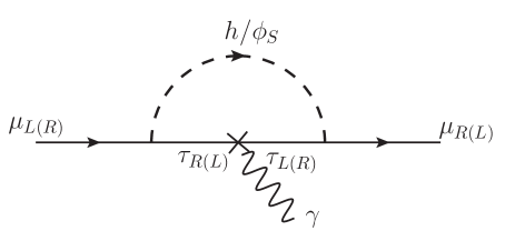
Figure 1: Sketched Feynman diagram for the Higgs- and $\phi_{S}$-mediated muon $g-2$.

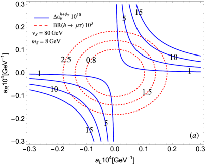
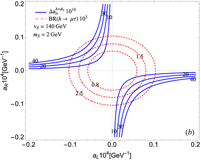
Figure 2: Contours for $BR(h\to\mu\tau)$ in units of $10^{-3}$ (dashed) and $\Delta a_{\mu}^{h+\phi_{S}}$ in units of $10^{-10}$ (solid) as a function of $a_{R}$ and $a_{L}$, where $(v_{S},m_{S})=(80,8)$ GeV in plot (a) and $(v_{S},m_{S})=(140,2)$ GeV in plot (b) are taken.

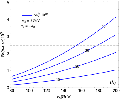
Figure 3: Contours for $\Delta a_{\mu}^{\phi_{S}}$ (in units of $10^{-10}$) as a function of $BR(h\to\mu\tau)$ and $v_{S}$, where $m_{S}=8$ GeV and $a_{L}=a_{R}$ are used in plot (a), $m_{S}=2$ GeV and $a_{L}=-a_{R}$ are used in plot (b), and the dashed line is the upper limit from CMS CMS:2017onh .

Basically, $a_{R}$ and $a_{L}$ appearing in Eqs. (55) and (59) can be taken as two independent parameters; however, if we use the scheme with $a_{L}\approx\pm a_{R}$, $\Delta a_{\mu}^{h+\phi_{S}}$ can be expressed in terms of $BR(h\to\mu\tau)$ as:

$$\frac{\Delta a_{\mu}^{h+\phi_{S}}}{BR(h\to\mu\tau)}\approx\pm\frac{m_{\mu}m_{\tau}\Gamma_{h}}{\pi m^{3}_{h}}\left[\left(\ln\frac{m^{2}_{h}}{m^{2}_{\tau}}-\frac{3}{2}\right)+\frac{(vm_{h})^{2}}{(m_{S}v_{S})^{2}}\left(\ln\frac{m^{2}_{S}}{m^{2}_{\tau}}-\frac{3}{2}\right)\right]\,.$$ (60)

Since there is no other free parameter in the first term of Eq. (60), if we take the CMS upper limit with $BR(h\to\mu\tau)\sim 2.5\times 10^{-3}$, the Higgs contribution can be estimated to be $\Delta a^{h}_{\mu}\sim 2.2\times 10^{-12}$, which is far below the current experimental value. Hence, the dominant contribution to $\Delta a_{\mu}^{h+\phi_{S}}$ is from the $\phi_{S}$ mediation. For simplicity, we take $\Delta a_{\mu}^{h+\phi_{S}}\simeq\Delta a_{\mu}^{\phi_{S}}$ in our analysis. Based on Eq. (60), we show the contours for $\Delta a_{\mu}^{\phi_{S}}$ (in units of $10^{-10})$ as a function of $BR(h\to\mu\tau)$ and $v_{S}$ in Fig. 3(a) and Fig. 3(b), where the former plot corresponds to $m_{S}=8$ GeV and $a_{L}=a_{R}$, the latter plot is $m_{S}=2$ GeV and $a_{L}=-a_{R}$, and the dashed line in both plots denotes the CMS upper limit. From the plots, it can be seen that when the value of $BR(h\to\mu\tau)$ is around $1\times 10^{-3}$, the value of $\Delta a_{\mu}^{\phi_{S}}$ can still reach $10\times 10^{-10}$.

In order to clearly see the influence of the $\phi_{S}$-mediated effects on the muon $g-2$, we show the contours for $\Delta a_{\mu}^{\phi_{S}}$ as a function of $m_{Z^{\prime}}$ and $g_{Z^{\prime}}$ in Fig. 4, where $v_{S}=m_{Z^{\prime}}/(2g_{Z^{\prime}})$, $BR(h\to\mu\tau)=1\times 10^{-3}$, $m_{S}=8$ GeV in plot (a), and $m_{S}=2$ GeV in plot (b) are used; the results bounded by the dot-dashed, dashed, and solid lines represent the contributions from the $Z^{\prime}$ boson, $\phi_{S}$, and $Z^{\prime}+\phi_{S}$, respectively; the taken region for each contribution is given by $\Delta a^{Z^{\prime}}_{\mu}=(2,8)\times 10^{-10}$, $\Delta a^{\phi_{S}}_{\mu}=(1,10)\times 10^{-10}$, and $\Delta a^{Z^{\prime}+\phi_{S}}_{\mu}=(12.7,44.7)\times 10^{-10}$. ; and the $Z^{\prime}$ contribution is written as Eq. (58). Since $\Delta a^{\phi_{S}}_{\mu}\propto BR(h\to\mu\tau)/v^{2}_{S}=4g^{2}_{Z^{\prime}}BR(h\to\mu\tau)/m^{2}_{Z^{\prime}}$, when $m_{Z^{\prime}}$ approaches the region of $m_{Z^{\prime}}\ll 1$ GeV, $g_{Z^{\prime}}$ must decrease in order to keep $\Delta a^{\phi_{S}}_{\mu}$ constant. This behavior is different from the $Z^{\prime}$-mediated muon $g-2$, where $\Delta a^{Z^{\prime}}_{\mu}$ approaches a constant when $m_{Z^{\prime}}$ goes to zero. According to the plots, if the $Z^{\prime}$-mediated muon $g-2$ is $\Delta a^{Z^{\prime}}_{\mu}<10\times 10^{-10}$ at $g_{Z^{\prime}}\sim{\cal O}(10^{-3})$, the muon $g-2$ can be enhanced to the current data with $2\sigma$ errors when the $\phi_{S}$ contribution is included.

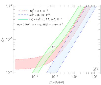
Figure 4: Contours for $\Delta a_{\mu}$ with (a) $m_{S}=8$ GeV and $a_{L}=a_{R}$ and (b) $m_{S}=2$ GeV and $a_{L}=-a_{R}$ as a function of $m_{Z^{\prime}}$ and $g_{Z^{\prime}}$, where the results bounded by the dot-dashed, dashed, and solid lines denote the $Z^{\prime}$, $\phi_{S}$, and $Z^{\prime}+\phi_{S}$ contributions, respectively.

III.2 $Z^{\prime}$ and rare $\tau$ decays

As shown above, in order to enhance the muon $g-2$ up to the $10^{-10}-10^{-9}$ level, a light $\phi_{S}$ is preferred. In this situation, the $\phi_{S}$ predominantly decays into $\tau\mu$ and $Z^{\prime}Z^{\prime}$. According to the gauge coupling in Eq. (9) and the Yukawa couplings in Eq. (36), the $\phi_{S}$ partial decay rates can be expressed as:

$$\Gamma(\phi_{S}\to Z^{\prime}Z^{\prime}) =\frac{m^{3}_{S}}{16\pi v^{2}_{S}}\,,$$

$$\Gamma(\phi_{S}\to\tau\mu) =\frac{v^{2}\left(|a_{L}|^{2}+|a_{R}|^{2}\right)}{8\pi}m_{S}\,,$$

$$=8.3\times 10^{-8}\frac{m_{S}v^{2}}{v^{2}_{S}}\frac{BR(h\to\tau\mu)}{2.5\times 10^{-3}}\,,$$ (61)

where the lepton and $Z^{\prime}$ mass effects are neglected, and $\tau\mu$ indicates the sum of the $\bar{\tau}\mu$ and $\bar{\mu}\tau$ channels. In the last line, we applied the result of Eq. (56). It can be clearly seen that $\Gamma(\phi_{S}\to\tau\mu)\ll\Gamma(\phi_{S}\to Z^{\prime}Z^{\prime})$. Accordingly, the BRs for the $\phi_{S}$ decays are shown as:

$$BR(\phi_{S}\to Z^{\prime}Z^{\prime}) \approx 1\,,$$

$$BR(\phi_{S}\to\tau\mu) \approx 2.57\times 10^{-3}\left(\frac{10\,\rm GeV}{m_{S}}\right)^{2}\frac{BR(h\to\mu\tau)}{2.5\times 10^{-3}}\,.$$ (62)

In addition to the $\phi_{S}\to\tau\mu$ decay, the same LFV effects can lead to $\tau\to\mu Z^{\prime}Z^{\prime}$ decay through the $\phi_{S}$ mediation. The differential branching fraction as a function of $Z^{\prime}Z^{\prime}$ invariant mass is shown as:

$$\frac{dBR(\tau\to\mu Z^{\prime}Z^{\prime})}{dq^{2}} \approx\frac{m_{\tau}}{64\pi^{2}m_{h}}\frac{\Gamma_{h}}{\Gamma_{\tau}}BR(h\to\mu\tau)$$

$$\times\frac{(q^{2}-2m_{Z^{\prime}}^{2})^{2}+8m^{4}_{Z^{\prime}}}{v^{4}_{S}m^{2}_{S}}\left(1-\frac{q^{2}}{m^{2}_{\tau}}\right)^{2}\sqrt{1-\frac{4m^{2}_{Z^{\prime}}}{q^{2}}}\,.$$ (63)

Based on the result, we show the contours for $BR(\tau\to\mu Z^{\prime}Z^{\prime})$ (dot-dashed) as a function of $BR(h\to\mu\tau)$ and $v_{S}$ with $m_{Z^{\prime}}=0.25$ GeV in Fig. 5, where plot (a) denotes $m_{S}=8$ GeV and $a_{L}=a_{R}$, and plot (b) is $m_{S}=2$ GeV and $a_{L}=-a_{R}$. For comparison, we also show the muon $g-2$ (solid) in the plot (a) and (b), and the numbers on the contour lines denote the values of $BR(\tau\to\mu Z^{\prime}Z^{\prime})$ and $\Delta a_{\mu}^{\phi_{S}}$, which have been rescaled by a $10^{-8}$ and a $10^{-10}$ factor, respectively. From the plots, it can be seen that when $\Delta a_{\mu}^{\phi_{S}}$ is of the order of $10^{-10}$, the associated $BR(\tau\to\mu Z^{\prime}Z^{\prime})$ is in the order of $10^{-8}$.

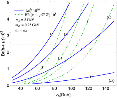
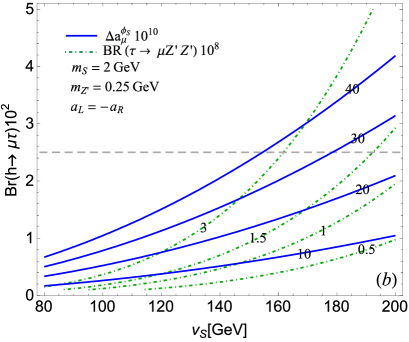
Figure 5: Contours for $BR(\tau\to\mu Z^{\prime}Z^{\prime})$ in units of $10^{-8}$ (dot-dashed) and $\Delta a_{\mu}^{\phi_{S}}$ in units of $10^{-10}$ (solid) with $m_{Z^{\prime}}=0.25$ GeV as a function of $BR(h\to\mu\tau)$ and $v_{S}$, where plot (a) denotes $m_{S}=8$ GeV and $a_{L}=a_{R}$, and the plot (b) is $m_{S}=2$ GeV and $a_{L}=-a_{R}$.

The possible detecting signals for $\tau\to\mu Z^{\prime}Z^{\prime}$ depend on the $Z^{\prime}$ mass. If $m_{Z^{\prime}}<2m_{\mu}$, the $Z^{\prime}$ gauge boson can only decay into $\nu_{\mu}$ and $\nu_{\tau}$ pairs. Thus, the detecting signals will be $\tau\to\mu+\not{E}$ with $\not{E}$ being a missing energy. Since the $\tau\to\mu\bar{\nu}_{\nu}\nu_{\tau}$ $BR\approx 17.27\%$ process in the SM is the main background, the small $BR(\tau\to\mu Z^{\prime}Z^{\prime})$ cannot be distinguished from the $BR^{\rm exp}(\tau\to\mu\bar{\nu}_{\nu}\nu_{\tau})=(17.39\pm 0.04)\%$ errors PDG . In this case, we cannot see the signal for the $\tau\to\mu Z^{\prime}Z^{\prime}$ decay. However, when $m_{Z^{\prime}}>2m_{\mu}$, in addition to the neutrino pair, the $Z^{\prime}$ can also decay into a muon pair. Therefore, the signals can be $\tau\to 3\mu\,\bar{\nu}\,\nu$ and $\tau\to 5\mu$, where $\nu$ includes the $\nu_{\mu}$ and $\nu_{\tau}$ neutrinos, and the decay chains are shown as:

$$\tau\to\mu Z^{\prime}Z^{\prime};Z^{\prime}\to\bar{\nu}\nu,\,Z^{\prime}\to\mu^{+}\mu^{-}$$ (64)

$$\tau\to\mu Z^{\prime}Z^{\prime};Z^{\prime}\to\mu^{+}\mu^{-},\,Z^{\prime}\to\mu^{+}\mu^{-}\,.$$ (65)

The BRs for the $Z^{\prime}\to(\bar{\nu}\nu,\mu^{+}\mu^{-})$ decays can be simply formulated as:

$$BR(Z^{\prime}\to\bar{\nu}\nu) =\frac{1}{1+M^{2}_{\mu}}\,,\quad BR(Z^{\prime}\to\mu^{+}\mu^{-})=\frac{M^{2}_{\mu}}{1+M^{2}_{\mu}}\,,$$ (66)

$$M^{2}_{\mu} =\left(1+\frac{2m^{2}_{\mu}}{m^{2}_{Z^{\prime}}}\right)\sqrt{1-\frac{4m^{2}_{\mu}}{m^{2}_{Z^{\prime}}}}\,,$$ (67)

where the BRs only depend on the $m_{Z^{\prime}}$ parameter. For illustration, we show the values of BRs with respect to some selected $m_{Z^{\prime}}$ values in Table 2. According to the results in Fig. 5 and the values shown in Table 2, it can be found that the BRs for $\tau\to(3\mu+\not{E},5\mu)$ can reach a level of $10^{-9}$, which is the detecting sensitivity at the Belle II Flores-Tlalpa:2015vga . In the Bell II experiment, $\tau$ leptons are produced in pairs and the signals of the $\tau$ decays could be $e^{+}e^{-}\to\tau(\to 3\mu+\not{E},5\mu)+\tau_{h}$, where $\tau_{h}$ is the hadronic $\tau$ decays. Thus, the SM background events are $(3\mu+\not{E},5\mu)+$ jet, which can be produced by the electroweak interactions. The background events can be reduced by applying proper kinematic cuts, such as the $\tau$ mass reconstruction from $3\mu+\not{E}$ or $5\mu$ in the final state, the muon-pair invariant mass distribution, and the various kinematic distributions of the same sign muons.

Table 2: Values of branching ratios for the $Z^{\prime}\to(\bar{\nu}\nu,\mu^{+}\mu^{-})$ decays with respect to the selected $m_{Z^{\prime}}$ values, where $\nu$ includes the $\nu_{\mu}$ and $\nu_{\tau}$ neutrinos.

$m_{Z^{\prime}}$ [GeV]	$0.22$	$0.25$	$0.3$	$0.34$	$0.38$
$BR(Z^{\prime}\to\bar{\nu}\nu)$	0.71	0.58	0.53	0.52	0.51
$BR(Z^{\prime}\to\mu^{+}\mu^{-})$	0.29	0.42	0.47	0.48	0.49

III.3 Influence on $e^{+}e^{-}\to\gamma Z^{\prime}$

Next, we examine the influence of vector-like leptons on the $e^{+}e^{-}\to\gamma Z^{\prime}$ process, which arises from the kinetic mixing Araki:2017wyg . The Feynman diagram for the loop-induced kinetic mixing is sketched in Fig. (7), where the leptons inside the loop include $\ell^{\prime}=\mu,\tau,\tau^{\prime}$, and $\tau^{\prime\prime}$. Accordingly, the effective Lagrangian is expressed as:

$${\cal L}_{\rm mix} =-\frac{\epsilon}{2}F_{\mu\nu}Z^{\prime\mu\nu}\,,$$

$$=-\Pi(q^{2})\left(q^{2}\epsilon_{\gamma}\cdot\epsilon^{*}_{Z^{\prime}}-q\cdot\epsilon_{\gamma}q\cdot\epsilon^{*}_{Z^{\prime}}\right)\,,$$ (68)

where $F_{\mu\nu}$ and $Z^{\prime}_{\mu\nu}$ are the $U(1)_{\rm em}$ and $U(1)_{\mu-\tau}$ gauge field strength tensors, respectively, and the $\epsilon=\Pi(q^{2})$ can be derived as:

$$\Pi(q^{2})=\frac{8eg_{Z^{\prime}}}{(4\pi)^{2}}\int^{1}_{0}dx\,x(1-x)\left[\ln\frac{m^{2}_{\tau}-x(1-x)q^{2}}{m^{2}_{\mu}-x(1-x)q^{2}}+\ln\frac{m^{2}_{L2}-x(1-x)q^{2}}{m^{2}_{L1}-x(1-x)q^{2}}\right]\,.$$ (69)

Since the $U(1)_{\mu-\tau}$ charges of $\ell_{4}$ and $\ell_{5}$ are opposite in sign, the scale-dependent factor from a renormalization scheme is cancelled, and the contributions of the vector-like leptons are basically similar to those of $\mu$ and $\tau$ leptons. In order to present the influence of $\tau^{\prime}$ and $\tau^{\prime\prime}$, we show the $\epsilon$ as a function of $E_{\gamma}$ in Fig. 7, where the relation of $E_{\gamma}$ and $q^{2}$ is given by $E_{\gamma}=(s-q^{2})/(2\sqrt{s})$; $\sqrt{s}$ is the center-of-mass energy of $e^{+}e^{-}$, and $\sqrt{s}=10.58$ GeV is used. In the left panel, the solid, dashed, dotted, and dot-dashed lines denote the results of $m_{L2}=(0.7,\,0.9,\,1.1,\,1.5)$ TeV, respectively, and $m_{L1}=0.7$ TeV is fixed. The horizontal lines denote the same situations for the $\epsilon_{\nu e}$ results. In the right panel, we fix $m_{L2}=0.7$ TeV and show the results with $m_{L1}=(0.7,\,0.9,\,1.1,\,1.5)$ TeV for $\epsilon$ and $\epsilon_{\nu e}$. We note that the results with $m_{L1}=m_{L2}=0.7$ TeV (solid) are the same as those without vector-like leptons. From the plots, it can be seen that $\epsilon$ in the small $E_{\gamma}$ region (i.e., larger $m_{Z^{\prime}}$) is sensitive to the ratio $m_{L2}/m_{L1}$. However, for the $e^{+}e^{-}\to\gamma+\not{E}$ process, the SM backgrounds dominate in the small $E_{\gamma}$ region. To clearly understand how the $q^{2}=m^{2}_{Z^{\prime}}$, $(m_{L_{1}}$, and $m_{L_{2}})$ affect the discovery significance, with the selected values of $\sqrt{q^{2}}=m_{Z^{\prime}}$ and $(m_{L_{1}},m_{L_{2}})$, we show the numerical values for the signal ($N_{S}$) and background ($N_{B}$) numbers and the corresponding significance, defined by $N_{S}/\sqrt{N_{B}+N_{S}}$, in Table 3, where $g_{Z^{\prime}}=10^{-3}$ is fixed and the integrated luminosity of 50 ab^-1 is used in the numerical calculations; here we applied formulas for the signal and SM background cross section in Ref. Araki:2017wyg . It can be found that the significance can be over $3\sigma$ as $m_{Z^{\prime}}\lesssim 1.0$ GeV and is increased(decreased) for $m_{L_{1}}<(>)\ m_{L_{2}}$.

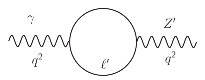
Figure 6: Sketched Feynman diagram for the kinetic mixing of $\gamma$ and $Z^{\prime}$, where the leptons inside the loop include $\ell^{\prime}=\mu,\tau,\tau^{\prime}$, and $\tau^{\prime\prime}$.

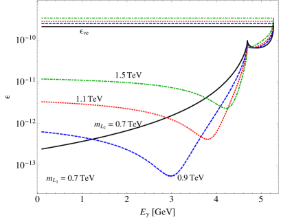
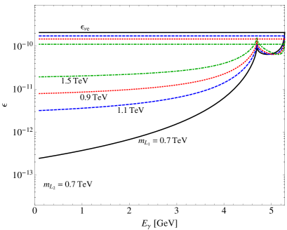
Figure 7: Left panel: $\epsilon$ for $m_{L2}>m_{L1}$ in Eq. (69) as a function of $E_{\gamma}$, where $E_{\gamma}=(s-q^{2})/(2\sqrt{s})$, and $\sqrt{s}=10.58$ GeV and $m_{L1}=0.7$ TeV are used; the solid, dashed, dotted, and dot-dashed lines denote the results of $m_{L2}=(0.7,0.9,1.1,1.5)$ TeV, respectively. The horizontal lines are the same situations but for the case of $\epsilon_{\nu e}=\Pi(0)$. The contributions of $m_{L1}=m_{L2}=0.7$ TeV are the same as for those without vector-like leptons. Right panel: the legend is the same as that in the left panel, but for $m_{L1}>m_{L2}$.

Table 3: Number of signal events $N_{S}$ and corresponding significance, defined by $N_{S}/\sqrt{N_{S}+N_{B}}$, for several taken values of $(m_{L_{1}},m_{L_{2}})$, where $g_{Z^{\prime}}=10^{-3}$ is fixed; the integrated luminosity of 50 ab^-1 is used, and the cases for $\sqrt{q^{2}}=m_{Z^{\prime}}=(1.0,1.5)$ GeV are presented. The number of background events is $N_{B}=8(30)$ for $m_{Z^{\prime}}=1.0(1.5)$ GeV.

$(m_{L_{1}},m_{L_{2}})$ [TeV]	$(0.7,0.7)$	$(0.7,1.1)$	$(0.7,1.5)$	$(1.1,0.7)$	$(1.5,0.7)$
$N_{S}$	14 (11)	19 (14)	23 (17)	11 (9)	9 (8)
Significance	3.0 (1.7)	3.6 (2.1)	4.1 (2.5)	2.5 (1.4)	2.2 (1.3)

III.4 Collider signatures

Two heavy vector-like leptons $\tau^{\prime}$ and $\tau^{\prime\prime}$ are introduced to generate the LFV scalar decays in this paper; therefore, it is of interest to study the production of the heavy leptons at the LHC. Since event simulation is beyond the scope of this paper, in the following we briefly discuss the potential channels and their production cross-sections.

In addition to the interactions of the $Z/\gamma$ gauge bosons and $\tau^{\prime}(\tau^{\prime\prime})$, from Eqs. (48), (86), and (100), we also have the flavor-changing couplings, expressed as:

$$\mu-\tau^{\prime}-Z:~{}\frac{gyy_{\mu}}{2\sqrt{2}c_{W}m_{L1}}\,,\quad\mu-\tau^{\prime\prime}-Z:~{}\frac{gyy^{\prime}_{\tau}}{2\sqrt{2}c_{W}m_{L2}}\,,$$

$$\mu-\tau^{\prime}-h:~{}\frac{y_{\mu}}{\sqrt{2}}\,,\quad\quad\quad\quad~{}~{}\tau-\tau^{\prime}-\phi_{S}:~{}\frac{y_{\tau}}{\sqrt{2}}\,,$$

$$\tau-\tau^{\prime\prime}-h:~{}\frac{y^{\prime}_{\tau}}{\sqrt{2}}\,,\quad\quad\quad\quad~{}~{}\mu-\tau^{\prime\prime}-\phi_{S}:~{}\frac{y^{\prime}_{\mu}}{\sqrt{2}}\,.$$ (70)

Therefore, the heavy leptons can be produced through the single and pair production channels. For singlet $\tau^{\prime}(\tau^{\prime\prime})$ production, the main processes in $pp$ collisions are from $q\bar{q}\to Z^{*}\to\tau^{\prime}\mu(\tau^{\prime\prime}\tau)$ and $gg\to h^{*}\to\tau^{\prime}\mu(\tau^{\prime\prime}\tau)$. The $\tau^{\prime}(\tau^{\prime\prime})$ pair production processes are via the $Z/\gamma$ gauge boson exchange. Using CalcHEP 3.6 Belyaev:2012qa with CTEQ6 parton distribution functions (PDFs) Nadolsky:2008zw , the single $\tau^{\prime}/\tau^{\prime\prime}$ and $\tau^{\prime}/\tau^{\prime\prime}$ pair production cross-sections with $m_{\tau^{\prime}(\tau^{\prime\prime})}=(0.7,0.9,1.1)$ TeV and $y_{\mu}\sim y^{\prime}_{\tau}\sim 1$ at $\sqrt{s}=13$ TeV are shown in Table 4, where we have used a K-factor of 1.5 for $gg\to h^{*}\to\tau^{\prime}\mu(\tau^{\prime\prime}\tau)$. We note that the values of the single and pair production cross-sections accidentally are the same due to the use of $y_{\mu}\sim y^{\prime}_{\tau}\sim 1$.

Table 4: Single $\tau^{\prime}/\tau^{\prime\prime}$ and $\tau^{\prime}/\tau^{\prime\prime}$ pair production cross-sections at $\sqrt{s}=13$ TeV.

$m_{\tau^{\prime}/\tau^{\prime\prime}}$ [TeV]	$0.7$	$0.9$	$1.1$
$\sigma(\tau^{\prime}/\tau^{\prime\prime})$ [fb]	0.43	0.11	0.036
$\sigma(\tau^{\prime}\tau^{\prime}/\tau^{\prime\prime}\tau^{\prime\prime})$ [fb]	0.43	0.11	0.035

From Eq. (70), it can be clearly seen that the $\tau^{\prime}\to\mu Z$ and $\tau^{\prime\prime}\to\tau Z$ decays have the suppression factors $v/m_{L1,L2}$; therefore, the heavy lepton decaying to the Higgs and $\phi_{S}$ are the dominant channels. If we assume $y_{\mu}\sim y_{\tau}$ and $y^{\prime}_{\mu}\sim y^{\prime}_{\tau}$ and neglect the $m_{h,\phi_{S}}$ effects due to $m_{h,\phi_{S}}\ll m_{\tau^{\prime},\tau^{\prime\prime}}$, the BRs can be simplified to be $BR(\tau^{\prime}\to\mu h)\sim BR(\tau^{\prime}\to\tau\phi_{S})\sim BR(\tau^{\prime\prime}\to\tau h)\sim BR(\tau^{\prime\prime}\to\mu\phi_{S})\sim 1/2$. Since $\phi_{S}$ has not yet been observed, the better discovery channels are through the Higgs production; accordingly, the collider signatures can be expressed as:

$$pp\to\bar{\tau}^{\prime}\mu(\bar{\tau}^{\prime\prime}\tau)\to\bar{\mu}\mu h(\bar{\tau}\tau h)\,,$$

$$pp\to\bar{\tau}^{\prime}\tau^{\prime}(\bar{\tau}^{\prime\prime}\tau^{\prime\prime})\to\bar{\mu}\mu hh(\bar{\tau}\tau hh)\,.$$ (71)

With the luminosity of 300 fb^-1 and $m_{\tau^{\prime}(\tau^{\prime\prime})}=0.7$ TeV, the event numbers for the single and pair production are estimated as 65 and 32, respectively. Since the discovery significance depends on the background events and kinematic analysis, we leave the detailed study for future work.

IV Summary

We studied the $U(1)_{L_{\mu}-L_{\tau}}$ extension of the SM by including a pair of singlet vector-like leptons, where both heavy leptons carry different $L_{\mu}-L_{\tau}$ charges. We employ a complex singlet scalar field to dictate the spontaneous $U(1)_{L_{\mu}-L_{\tau}}$ symmetry breaking. With $g_{Z^{\prime}}\sim O(10^{-3})$, the VEV of the singlet scalar field must be at the electroweak scale in order to obtain $m_{Z^{\prime}}$ in the MeV to GeV region. It is found that the scalar boson contributions to the muon $g-2$ and the $h\to\mu\tau$ decay are strongly correlated in this model when the condition $a_{L}\simeq a_{R}$ is assumed. As a result, when $BR(h\to\mu\tau)\sim 10^{-3}$ is taken, the scalar-mediated muon $g-2$ can reach $10\times 10^{-10}$. Moreover, even with $g_{Z^{\prime}}\sim 10^{-4}$, the muon $g-2$ combining $Z^{\prime}$ and $\phi_{S}$ contributions can fit the current data with $2\sigma$ errors. The kinetic mixing in the $e^{+}e^{-}\to\gamma+\not{E}$ process not only depends on the $q^{2}=m^{2}_{Z^{\prime}}$, but also is sensitive to the ratio of $m_{L2}/m_{L1}$; as a result, the significance of discovering the signal of $e^{+}e^{-}\to\gamma\not{E}$ increases (decreases) for $m_{L2}>(<)\ m_{L1}$. It is found that $BR(\tau\to\mu Z^{\prime}Z^{\prime})$ by the $\phi_{S}$ mediation can be of the ${\cal O}(10^{-8})$. When the BRs for $Z^{\prime}\to(\bar{\nu}\nu,\mu^{+}\mu^{-})$ are included, $BR(\tau\to 3\mu+\not{E},5\mu)$ of $10^{-9}$ can fall within the sensitivity of Belle II experiment in the search for the rare tau decays. In addition, we briefly discuss the collider signatures for discovering the heavy leptons $\tau^{\prime}$ and $\tau^{\prime\prime}$. The promising channels are through the Higgs production and given as $pp\to\bar{\mu}\mu(\bar{\tau}\tau)h$ and $pp\to\bar{\mu}\mu(\bar{\tau}\tau)hh$.

Acknowledgments

This work was partially supported by the Ministry of Science and Technology of Taiwan, under grant MOST-103-2112-M-006-004-MY3 (CHC).

Appendix

The Higgs Yukawa couplings in Eq. (35) is written as:

$$-{\cal L}_{h} =\left(\begin{array}[]{cc}\boldsymbol{\bar{\ell}}_{L}\,,&\boldsymbol{\bar{\Psi}}_{\tau^{\prime}L}\end{array}\right)V_{L}\left(\begin{array}[]{c|c}~{}~{}~{}\boldsymbol{m_{\ell}}_{3\times 3}{}{}{}&\boldsymbol{\delta m_{1}}\\ \hline\cr 0&0\end{array}\right)V^{\dagger}_{R}\left(\begin{array}[]{c}\boldsymbol{\ell_{R}}\\ \boldsymbol{\Psi}_{\tau^{\prime}R}\end{array}\right)\frac{h}{v}+H.c.\,,$$ (77)

$$\approx\left(\begin{array}[]{ccc}\boldsymbol{\bar{\ell}}_{L}\,,&\boldsymbol{\bar{\Psi}}_{\tau^{\prime}L}\end{array}\right)\left(\begin{array}[]{c|c}\boldsymbol{m}_{\ell}-\boldsymbol{\delta m}_{1}\boldsymbol{\epsilon}^{\dagger}_{R}&\boldsymbol{\delta m_{1}}\\ \hline\cr 0&\boldsymbol{\epsilon}^{\dagger}_{L}\boldsymbol{\delta m}_{1}\end{array}\right)\left(\begin{array}[]{c}\boldsymbol{\ell_{R}}\\ \boldsymbol{\Psi}_{\tau^{\prime}R}\end{array}\right)\frac{h}{v}+H.c.\,,$$ (83)

where we have applied the flavor mixing matrices of Eq. (18) in the second line, and $\boldsymbol{\delta m}_{1}\boldsymbol{\epsilon}^{\dagger}_{R}$ and $\boldsymbol{\epsilon}^{\dagger}_{L}\boldsymbol{\delta m}_{1}$ are given by:

$$\boldsymbol{\delta m}_{1}\boldsymbol{\epsilon}^{\dagger}_{R}=\frac{vv_{S}}{2}\left(\begin{array}[]{ccc}0&0&0\\ 0&y_{\mu}y^{\prime}_{\mu}\left(-\frac{c_{\alpha}s_{\alpha}}{m_{L1}}+\frac{c_{\alpha}s_{\alpha}}{m_{L2}}\right)&y_{\mu}y_{\tau}\left(\frac{c^{2}_{\alpha}}{m_{L1}}+\frac{s^{2}_{\alpha}}{m_{L2}}\right)\\ 0&y^{\prime}_{\mu}y^{\prime}_{\tau}\left(\frac{s^{2}_{\alpha}}{m_{L1}}+\frac{c^{2}_{\alpha}}{m_{L2}}\right)&y_{\tau}y^{\prime}_{\tau}\left(-\frac{c_{\alpha}s_{\alpha}}{m_{L1}}+\frac{c_{\alpha}s_{\alpha}}{m_{L2}}\right)\end{array}\right)\,,$$ (84)

$$\boldsymbol{\epsilon}^{\dagger}_{L}\boldsymbol{\delta m}_{1}=\frac{v^{2}}{2}\left(\begin{array}[]{cc}\frac{y^{2}_{\mu}c^{2}_{\alpha}+y^{\prime 2}_{\tau}s^{2}_{\alpha}}{m_{L1}}&\frac{y^{2}_{\mu}-y^{\prime 2}_{\tau}}{m_{L1}}c_{\alpha}s_{\alpha}\\ \frac{y^{2}_{\mu}-y^{\prime 2}_{\tau}}{m_{L2}}c_{\alpha}s_{\alpha}&\frac{y^{2}_{\mu}s^{2}_{\alpha}+y^{\prime 2}_{\tau}c^{2}_{\alpha}}{m_{L2}}\end{array}\right)\,.$$ (85)

Hence, the Higgs couplings to the charged leptons can be decomposed as:

$$-{\cal L}_{h} =\frac{m_{\ell}}{v}\bar{\ell}_{L}\ell_{R}h+\frac{v_{S}c_{\alpha}s_{\alpha}}{2}\frac{m_{L2}-m_{L1}}{m_{L1}m_{L2}}\left(y_{\mu}y^{\prime}_{\mu}\bar{\mu}_{L}\mu_{R}+y_{\tau}y^{\prime}_{\tau}\bar{\tau}_{L}\tau_{R}\right)h$$

$$-\frac{v_{S}y_{\mu}y_{\tau}}{2}\left(\frac{c^{2}_{\alpha}}{m_{L1}}+\frac{s^{2}_{\alpha}}{m_{L2}}\right)\bar{\mu}_{L}\tau_{R}h-\frac{v_{S}y^{\prime}_{\mu}y^{\prime}_{\tau}}{2}\left(\frac{s^{2}_{\alpha}}{m_{L1}}+\frac{c^{2}_{\alpha}}{m_{L2}}\right)\bar{\tau}_{L}\mu_{R}h$$

$$+\frac{y_{\mu}}{\sqrt{2}}\bar{\mu}_{L}\left(c_{\alpha}\tau^{\prime}_{R}+s_{\alpha}\tau^{\prime\prime}_{R}\right)h+\frac{y^{\prime}_{\tau}}{\sqrt{2}}\bar{\tau}_{L}\left(-s_{\alpha}\tau^{\prime}_{R}+c_{\alpha}\tau^{\prime\prime}_{R}\right)h+\boldsymbol{\bar{\Psi}}_{\tau^{\prime}L}\boldsymbol{\epsilon}^{\dagger}_{L}\boldsymbol{\delta m}_{1}\boldsymbol{\Psi}_{\tau^{\prime}R}\frac{h}{v}+H.c.$$ (86)

Similarly, the $\phi_{S}$ Yukawa couplings in Eq. (35) is expressed as:

$$-{\cal L}_{\phi_{S}} =\left(\begin{array}[]{cc}\boldsymbol{\bar{\ell}}_{L}\,,&\boldsymbol{\bar{\Psi}}_{\tau^{\prime}L}\end{array}\right)V_{L}\left(\begin{array}[]{c|c}~{}~{}~{}0{}{}{}&0\\ \hline\cr\boldsymbol{\delta m^{T}_{2}}&0\end{array}\right)V^{\dagger}_{R}\left(\begin{array}[]{c}\boldsymbol{\ell_{R}}\\ \boldsymbol{\Psi}_{\tau^{\prime}R}\end{array}\right)\frac{\phi_{S}}{v_{S}}\,,$$ (92)

$$\approx\left(\begin{array}[]{cc}\boldsymbol{\bar{\ell}}_{L}\,,&\boldsymbol{\bar{\Psi}}_{\tau^{\prime}L}\end{array}\right)V_{L}\left(\begin{array}[]{c|c}-\boldsymbol{\epsilon}_{L}\boldsymbol{\delta m}^{T}_{2}&0\\ \hline\cr\boldsymbol{\delta m}^{T}_{2}&\boldsymbol{\delta m}^{T}_{2}\boldsymbol{\epsilon}_{R}\end{array}\right)V^{\dagger}_{R}\left(\begin{array}[]{c}\boldsymbol{\ell_{R}}\\ \boldsymbol{\Psi}_{\tau^{\prime}R}\end{array}\right)\frac{\phi_{S}}{v_{S}}\,,$$ (98)

where $\boldsymbol{\epsilon}_{L}\boldsymbol{\delta m}^{T}_{2}=\boldsymbol{\delta m}_{1}\boldsymbol{\epsilon}^{\dagger}_{R}$, and $\boldsymbol{m}^{T}_{2}\boldsymbol{\epsilon}_{R}$ is written as:

$$\boldsymbol{m}^{T}_{2}\boldsymbol{\epsilon}_{R}=\frac{v^{2}_{S}}{2}\left(\begin{array}[]{cc}\frac{y^{\prime 2}_{\mu}s^{2}_{\alpha}+y^{2}_{\tau}c^{2}_{\alpha}}{m_{L1}}&\frac{-y^{\prime 2}_{\mu}+y^{2}_{\tau}}{m_{L2}}c_{\alpha}s_{\alpha}\\ \frac{-y^{\prime 2}_{\mu}+y^{2}_{\tau}}{m_{L1}}c_{\alpha}s_{\alpha}&\frac{y^{\prime 2}_{\mu}c^{2}_{\alpha}+y^{2}_{\tau}s^{2}_{\alpha}}{m_{L2}}\end{array}\right)\,.$$ (99)

Then, the $\phi_{S}$ Yukawa couplings to the charged leptons can be written as:

$$-{\cal L}_{\phi_{S}} =\frac{vc_{\alpha}s_{\alpha}}{2}\frac{m_{L2}-m_{L1}}{m_{L1}m_{L2}}\left(y_{\mu}y^{\prime}_{\mu}\bar{\mu}_{L}\mu_{R}+y_{\tau}y^{\prime}_{\tau}\bar{\tau}_{L}\tau_{R}\right)\phi_{S}-\frac{vy_{\mu}y_{\tau}}{2}\left(\frac{c^{2}_{\alpha}}{m_{L1}}+\frac{s^{2}_{\alpha}}{m_{L2}}\right)\bar{\mu}_{L}\tau_{R}\phi_{S}$$

$$-\frac{vy^{\prime}_{\mu}y^{\prime}_{\tau}}{2}\left(\frac{s^{2}_{\alpha}}{m_{L1}}+\frac{c^{2}_{\alpha}}{m_{L2}}\right)\bar{\tau}_{L}\mu_{R}\phi_{S}+\frac{y^{\prime}_{\mu}}{\sqrt{2}}\left(-s_{\alpha}\bar{\tau}^{\prime}_{L}+c_{\alpha}\bar{\tau}^{\prime\prime}_{L}\right)\mu_{R}\phi_{S}$$

$$+\frac{y_{\tau}}{\sqrt{2}}\left(c_{\alpha}\bar{\tau}^{\prime}_{L}+s_{\alpha}\bar{\tau}^{\prime\prime}_{L}\right)\tau_{R}\phi_{S}+\boldsymbol{\bar{\Psi}}_{\tau^{\prime}L}\boldsymbol{\delta m}^{T}_{2}\boldsymbol{\epsilon}_{R}\boldsymbol{\Psi}_{\tau^{\prime}R}\frac{\phi_{S}}{v_{S}}+H.c.$$ (100)

References

- (1) X. G. He, G. C. Joshi, H. Lew and R. R. Volkas, Phys. Rev. D 43, 22 (1991).
- (2) R. Foot, X. G. He, H. Lew and R. R. Volkas, Phys. Rev. D 50, 4571 (1994) [hep-ph/9401250].
- (3) S. N. Gninenko and N. V. Krasnikov, Phys. Lett. B 513, 119 (2001) [hep-ph/0102222].
- (4) S. N. Gninenko, N. V. Krasnikov and V. A. Matveev, Phys. Rev. D 91, 095015 (2015) [arXiv:1412.1400 [hep-ph]].
- (5) W. Altmannshofer, C. Y. Chen, P. S. Bhupal Dev and A. Soni, Phys. Lett. B 762, 389 (2016) [arXiv:1607.06832 [hep-ph]].
- (6) M. G. Aartsen et al. [IceCube Collaboration], Phys. Rev. Lett. 113, 101101 (2014) [arXiv:1405.5303 [astro-ph.HE]].
- (7) T. Araki, F. Kaneko, Y. Konishi, T. Ota, J. Sato and T. Shimomura, Phys. Rev. D 91, no. 3, 037301 (2015) [arXiv:1409.4180 [hep-ph]].
- (8) A. Kamada and H. B. Yu, Phys. Rev. D 92, no. 11, 113004 (2015) [arXiv:1504.00711 [hep-ph]].
- (9) A. DiFranzo and D. Hooper, Phys. Rev. D 92, no. 9, 095007 (2015) [arXiv:1507.03015 [hep-ph]].
- (10) T. Araki, F. Kaneko, T. Ota, J. Sato and T. Shimomura, Phys. Rev. D 93, no. 1, 013014 (2016) [arXiv:1508.07471 [hep-ph]].
- (11) W. Altmannshofer, S. Gori, M. Pospelov and I. Yavin, Phys. Rev. D 89, 095033 (2014) [arXiv:1403.1269 [hep-ph]].
- (12) A. Crivellin, G. D’Ambrosio and J. Heeck, Phys. Rev. Lett. 114, 151801 (2015) [arXiv:1501.00993 [hep-ph]].
- (13) W. Altmannshofer, S. Gori, S. Profumo and F. S. Queiroz, JHEP 1612, 106 (2016) [arXiv:1609.04026 [hep-ph]].
- (14) J. Heeck, M. Holthausen, W. Rodejohann and Y. Shimizu, Nucl. Phys. B 896, 281 (2015) [arXiv:1412.3671 [hep-ph]].
- (15) J. Heeck, Phys. Lett. B 758, 101 (2016) [arXiv:1602.03810 [hep-ph]].
- (16) W. Altmannshofer, M. Carena and A. Crivellin, Phys. Rev. D 94, no. 9, 095026 (2016) [arXiv:1604.08221 [hep-ph]].
- (17) S. Baek, H. Okada and K. Yagyu, JHEP 1504, 049 (2015) [arXiv:1501.01530 [hep-ph]].
- (18) S. Baek, Phys. Lett. B 756, 1 (2016) [arXiv:1510.02168 [hep-ph]].
- (19) S. Patra, S. Rao, N. Sahoo and N. Sahu, Nucl. Phys. B 917, 317 (2017) [arXiv:1607.04046 [hep-ph]].
- (20) A. Biswas, S. Choubey and S. Khan, JHEP 1609, 147 (2016) [arXiv:1608.04194 [hep-ph]].
- (21) S. Lee, T. Nomura and H. Okada, arXiv:1702.03733 [hep-ph].
- (22) D. Geiregat et al. [CHARM-II Collaboration], Phys. Lett. B 245, 271 (1990).
- (23) S. R. Mishra et al. [CCFR Collaboration], Phys. Rev. Lett. 66, 3117 (1991).
- (24) W. Altmannshofer, S. Gori, M. Pospelov and I. Yavin, Phys. Rev. Lett. 113, 091801 (2014) [arXiv:1406.2332 [hep-ph]].
- (25) J. P. Lees et al. [BaBar Collaboration], Phys. Rev. D 94, no. 1, 011102 (2016) [arXiv:1606.03501 [hep-ex]].
- (26) R. Harnik, J. Kopp and P. A. N. Machado, JCAP 1207, 026 (2012) [arXiv:1202.6073 [hep-ph]].
- (27) G. Bellini et al., Phys. Rev. Lett. 107, 141302 (2011) [arXiv:1104.1816 [hep-ex]].
- (28) Y. Kaneta and T. Shimomura, arXiv:1701.00156 [hep-ph].
- (29) T. Araki, S. Hoshino, T. Ota, J. Sato and T. Shimomura, Phys. Rev. D 95, no. 5, 055006 (2017) [arXiv:1702.01497 [hep-ph]].
- (30) T. Aushev et al., arXiv:1002.5012 [hep-ex].
- (31) G. W. Bennett et al. [Muon g-2 Collaboration], Phys. Rev. D 73, 072003 (2006) [hep-ex/0602035].
- (32) J. Grange et al. [Muon g-2 Collaboration], arXiv:1501.06858 [physics.ins-det].
- (33) M. Otani [E34 Collaboration], JPS Conf. Proc. 8, 025008 (2015).
- (34) G. Aad et al. [ATLAS Collaboration], Eur. Phys. J. C 77, no. 2, 70 (2017) [arXiv:1604.07730 [hep-ex]].
- (35) V. Khachatryan et al. [CMS Collaboration], Phys. Lett. B 749 (2015) 337 [arXiv:1502.07400 [hep-ex]].
- (36) CMS Collaboration [CMS Collaboration], CMS-PAS-HIG-17-001.
- (37) C. Patrignani et al. (Particle Data Group), Chin. Phys. C, 40, 100001 (2016).
- (38) A. Flores-Tlalpa, G. Lopez Castro and P. Roig, JHEP 1604, 185 (2016) [arXiv:1508.01822 [hep-ph]].
- (39) A. Belyaev, N. D. Christensen and A. Pukhov, Comput. Phys. Commun. 184, 1729 (2013) [arXiv:1207.6082 [hep-ph]].
- (40) P. M. Nadolsky, H. L. Lai, Q. H. Cao, J. Huston, J. Pumplin, D. Stump, W. K. Tung and C.-P. Yuan, Phys. Rev. D 78, 013004 (2008) [arXiv:0802.0007 [hep-ph]].